Hybrid Deep Learning for Brain Tumor Detection: Combining DenseNet and Custom CNN for Enhanced Accuracy

Abstract

Background:

Deep learning in brain tumor detection has become an important breakthrough in medical imaging to facilitate a fast and accurate diagnosis. Conventional models such as VGG, SVM, and common CNNs are competitive, yet fail to provide the sensitivity and specificity needed in real-time diagnosis purposes.

Objectives:

The objective of the proposed study is to generate a hybrid deep learning architecture of the DenseNet and a self-developed Convolutional Neural Network (CNN) in order to increase the classification accuracy, sensitivity, and specificity of a brain tumor detection medical image.

Design:

A Hybrid architecture consisting of DenseNet feature reuse and connectivity with a domain-specific custom CNN is suggested to retrieve high-level semantic and fine-grained features. The design focuses on performance evaluation with respect to the state-of-the-art models and ensemble frameworks.

Methods:

The brain tumor data set was preprocessed, and the augmentation methods, such as translation and rotation, were applied. A training and testing subsets of the dataset were formed. The hybrid approach, formed by DenseNet layers and a self-created CNN model, was implemented and tested. The performance of the model was contrasted with that of other benchmark classifiers such as SVM and VGG, DenseNet (single), CNN ensembles, and Hybrid Ensembles.

Results:

The hybrid DenseNet-Custom CNN model was more accurate and had better classification results than the standard models. In particular, it surpassed the accuracy of SVM (96%), VGG (94%), DenseNet (92%), and Hybrid Ensemble models (~95.2%), while the FPS remained equivalent to SVM and substantially lower than VGG. It proved better sensitivity and specificity with better feature representation and interpretation, as it made more accurate tumor classification.

Conclusion:

Incorporating DenseNet with a custom CNN model can increase the capabilities of brain tumor detection in medical imaging. This hybrid performance can use both general-purpose deep learning and domain-specific feature engineering, and it provides a practical suggestion of the approach that involves a satisfactory solution in the diagnostic sense. It verifies that the combination of more than 2 methods is productive in enhancing the results of medical image classification activities.

Introduction

The human brain is a very complex organ tasked with the regulation of body activities, interpreting sensory input, and facilitating cognition. is composed of billions of interconnected neurons and support cells. ¹ Given this complexity, the brain is particularly vulnerable to various types of tumors, which can significantly impair neurological function. Brain tumors are characterized by uncontrolled and abnormal growth of tissue either around the brain or in the brain itself. ² These tumors are broadly classified into benign (non-cancerous) and malignant (cancerous) categories, both of which can pose serious health risks depending on their size and location. While benign tumors typically grow slowly and remain localized, they may still cause severe symptoms by compressing critical regions of the brain. ³ Malignant tumors, on the other hand, are more aggressive and invasive, often spreading to adjacent tissues and leading to complex clinical challenges.

The classification of brain tumors further extends into primary and secondary (metastatic) forms. Primary tumors originate within the brain itself, arising from different cell types such as glial cells (gliomas), meningeal cells (meningiomas), or pituitary tissue (pituitary adenomas). Secondary tumors originate in other parts of the body and metastasize to the brain, typically presenting with more aggressive behavior and poorer prognosis. The diversity in tumor morphology—such as shape, size, texture, and growth pattern—complicates the task of accurate detection and classification.

Early and proper prediction of brain tumors is essential in the earlier planning of the treatment and enhancing patient outcomes. ⁴ Medical imaging plays a central role in this process, particularly Magnetic Resonance Imaging (MRI), which offers superior soft tissue contrast without ionizing radiation. However, interpreting MRI scans is inherently challenging, especially during the early stages of tumor development when visual differences between healthy and diseased tissue may be subtle. ⁵ These challenges are compounded by inter-observer variability and the high volume of clinical data, making manual analysis time-consuming and error-prone. ⁶

Some of these limitations have been overcome using image processing techniques that enhance image quality, delineate the region of interest, that is, tumor, and extract discriminative features which include the shape, texture, and intensity of images. ⁷ However, handcrafted features and predetermined rules are commonly used in the traditional processing methods and hence, might fail to generalize when applied over different clinical situations. ML and DL approaches have become prominent alternative methods for the detection of brain tumors in the past years. These models can learn directional features directly on the image data, reducing the extent to which feature engineering is required to be undertaken manually. ⁸ Particularly, Convolutional Neural Networks (CNNs) have demonstrated excellent efficiency in image classification problems and also in medical imaging. Nevertheless, ordinary deep learning architectures can overfit to small datasets as well as render them unable to recognize the multidimensional structures of medical images. Although progress was made, a few challenges remained unresolved. ⁹ The current models usually have limitations because they require only pre-trained architectures or custom CNNs, which have their trade-offs regarding generalization, performance, and flexibility. In addition, the imbalance of classes in datasets and the inability to explain them remain challenges to clinical deployment. ¹⁰

To overcome these gaps, this endeavor presents a hybrid deep architecture that combines the representational power of an already trained DenseNet121 and the task-specific ability of an architecture-specific CNN. The hybrid architecture is supposed to mine dense and varied features, whereas the single-architecture approaches have weaknesses. A common problem with many classification systems is low classification rates, low generalization, and poor results when changes or inaccuracies are made. The proposed model would help address those issues better because their output is to: enhance classification rate, improve generalizability, and enhance robustness of the brain tumor detection based on MRI data. The key research findings are the following:

• The development of an innovative hybrid architecture, composed of DenseNet121 and a specific CNN that is completely efficient in the classification of brain tumors.

• Data augmentation: Use of intensive strategies to reduce the imbalance in the dataset and degrade the model’s robustness.

• Comparison with several existing models and empirical assessment, showing better accuracy, precision, and recall.

• Mathematical and architectural specifications to allow reproducibility and development of additional work in the field.

Although a lot has been done, it is not easy to detect brain tumors accurately and early enough, given that the shape, size, and location of the tumor varies, as well as human limitations of manual interpretation of the results. Available deep learning methods are limited to one of the other methods: pre-trained models or user-defined CNNs, yet the inability to generalize to different MRI scans on these methods is frequently reported. This paper presents a hybridized network including DenseNet and a specialized CNN in order to improve classifications. The aim is to enhance the detection accuracy, overcome the limitations of the individual models by providing a synergistic jack-of-all-trades architecture to brain MRI data.

The main contributions of this work are the following:

• A new hybrid framework that is a mixture of DenseNet121 and the custom CNN that deals with the task of classifying tumors based on brain MRI images.

• Comprehensive comparison to state-of-the-art methods with a better sensitivity and F1-score.

• Consideration of data augmentation methods to address the issue relating to limited classes and better generalizability.

Structure of the paper: This paper has been organized in a form that can help one to understand almost any research and conclusion. The second section will offer an in-depth literature review, sparking critical reflections on previous research and providing essential background for this empirical study. This paper will detail the proposed strategic approach, discussed in Section 3, and share creative methods or methodologies employed. Section 4 will conclude by focusing on the results and discussion, which involves a detailed evaluation of the experimental findings. Section 5 will conclude the paper with a summary of key findings, discuss their significance, and suggest topics for future research.

Literature Review

Traditional Machine Learning Approaches

Machine Learning (ML) techniques are additionally revolutionizing the areas of preventive medicine and medical diagnostics. In medical diagnostics, prompt brain tumor detection is critical to ensure proper treatment; hence, researchers have been increasingly utilizing Machine Learning (ML)/Deep Learning (DL) methodologies for diagnosis, particularly when using MRI. ¹¹ This section of the literature review presents an extensive overview of methodologies and architectures, including the metrics of performance, of other machine learning and deep learning methods used on the identification and classification of brain tumors.

Detection of Brain Tumors from MRI data has been a popular application area using traditional machine learning techniques. Those generally comprise feature extraction, selection, and exploitation of classifiers such as Support Vector Machines (SVM), K-nearest neighbors (k-NN), or neural networks. PSO ¹² was first used in segmentation and reported an unpublished accuracy greater than naive. However, these techniques have restrictions caused by the quality of the extracted feature and are often based on manually designed features. For example, Kumar et al ¹³ proposed speeding up the detection of brain tumors using a feature selection strategy with Iterative Bayesian Multivariate Deep Neural Learning (WCFS-IBMDNL). Although this approach was promising, its False Alarm Rates were high, thus necessitating the need to improve accuracy while at the same time reducing the overall reduction in false positives.

A straightforward technique for tumor detection is to use a trained Support Vector-Neural Network, again with Harmony-Crow Search (SVNN(HCS)) optimization. ¹⁴ This method gave an example of the potential for hybrid approaches combining standard classifiers and optimization techniques. Nevertheless, the approaches’ applicability to different types of brain tumors or clinical settings is restricted because of their dependence on certain datasets, such as the BRATS dataset. ¹⁵ In recent years, deep learning has emerged as a powerful approach for identifying and classifying brain tumors. Among its techniques, Convolutional Neural Networks (CNNs) have demonstrated notable success in automatically extracting features from raw MRI data and accurately diagnosing brain cancers.

CNN-Based Deep Learning Models

GoogLeNet, AlexNet, and VGGNet are 3 well-known CNN architectures that were used in the tri-architectural CNN framework ¹⁶ developed. Three categories of malignancies were identified using this framework: meningioma, glioma, and pituitary gland tumors. The study used the VGG16 architecture to obtain an outstanding accuracy of 98.69% by fine-tuning and freezing the layers of the model. The accuracy of the categorization was further improved by the application of data augmentation techniques. In a similar vein, Abdusalomov et al ¹⁷ used a CNN-based deep learning model for classifying brain tumor images. After testing 5 different models, the study found that the model with the best accuracy, 98.5% on training data and 84.19% on validation data, had a maximum pool layer, a RELU layer, and 64 hidden neurons.

The second noteworthy CNN-based study ¹⁸ concentrated on feature extraction with a modified CNN architecture. There were 5 learnable layers in the design, and a 3 × 3 convolutional kernel was used. Initially, this model’s classification accuracy was 81%; however, with the use of an Extreme Learning Machine (ELM), it was improved to 93.68%. The study did, however, also reveal limits in the classifier’s capacity to distinguish between photos of meningiomas and pituitaries, indicating the need for additional model improvement. The idea of deep transfer learning for brain tumor categorization was investigated in Deepak et al. ¹⁹ Pre-trained models were utilized in the study to extract features from MRI data, which were then used to train classification algorithms. With the use of a fivefold classification model, the study’s accuracy was 98%. The results demonstrated how transfer learning may be used to take advantage of pre-trained models, which perform better than manual region classification techniques and are useful in automating the classification process. In Mostafa et al, ²⁰ another hybrid method was proposed that classified malignant and benign tumor areas in brain imaging by combining CNN and Neutrosophy. The method’s 95.62% average success rate shows how well deep learning and sophisticated mathematical techniques may be combined. The study did point out that not all brain tumor types will benefit equally from the CNN feature selection process, highlighting the need for more adaptive and flexible feature selection methods. Similarly, Antony et al ²¹ used a modified Wndchrm-based classification system that combines CNNs with neighborhood distance metrics. With a high accuracy of 98.25%, this approach shows how merging deep learning architectures with conventional machine learning techniques can enhance classification performance.

Hybrid Deep Learning Models

Classifying brain tumors has advanced significantly since the authors ²² introduced Capsule Networks (CapsNets). CapsNets are very useful in medical imaging because they can capture the spatial hierarchy between simple and complex things. By altering the maps in the CapsNet convolution layer, the study was able to achieve an accuracy of 86.50%. CapsNets provide an alternative method of managing spatial relationships in images, which may be useful for more complicated classification problems, even though their performance is lower than that of some CNN-based models. Using MRI data, Balamurugan et al ²³ presented a method for categorizing Glioma pictures that used CNNs and Genetic Algorithms (GA). The proposed method automatically selected CNN structures using genetic algorithms to reach 90.9% accuracy for diagnosing Glioma images or detecting tumors between Glioma, Meningiomas, and Pituitary tumors with an average of 94.2% corresponding F1-score. The integration of dynamic learning systems and genetic algorithms in deep learning highlights the importance of evolutionary computing for optimization and enhancement.

A method to classify brain tumors has been extended to utilize 3D MRI data besides the slices of a typical MRI. The authors in Jyothi and Singh ²⁴ proposed a 3-dimensional convolutional neural network (CNN) for automatically grading gliomas, from multi-sequence MRI using regions of interest (ROI). This work demonstrated that 3D CNNs can be used to learn spatial and volumetric features from MRI data with 89.5% accuracy for glioma grading and 92.98% in the prediction of tumor regions. Provided a 3D whole-slice method with DenseNet as a feature extractor for each planar view from the raw (stacked) image in Lu et al. ²⁵ Then, in the case of classification, a Recurrent Neural Network (RNN) with Long Short-Term Memory (LSTM) Units was used. This hybrid 2D to 3D approach demonstrates that the fusion of CNNs and RNNs can be particularly useful in handling temporal dependencies for MRI data through a mean accuracy value of 92.13%. Based on the slicing and patching of MRI images. In Banerjee et al, ²⁶ Cyriac et al, ²⁷ Karthikeyan et al,^28,29 MRI image classification is performed using custom ConvNet models that the authors developed from scratch. For processing multiple MRI imaging sequences, the study used ConvNets and VGGNet, and it achieved an accuracy rate of 97%. These model-agnostic representations that were extracted and learned brought to light the disadvantages of using feature extraction on pre-trained models, as they may not be well-suited for natural photos as much as medical images.

Transformer-Based and Attention Models

Transformer-based models have appeared in the field of medical image analysis as an alternative to the traditional CNNs in recent years and have proven their efficiency. The Swin Transformer stands out among them and brings the hierarchical structure with shifted windows that allow the efficient representation of long-range dependencies, but retain the computational efficiency. TransUNet uses transformer decoders together with CNN-based encoders and has the benefit of both local feature extraction and global context modeling, which is especially handy in segmenting and detecting tumor boundaries. The models have proved to be of high quality toward the characterization of irregular tumor shapes and handling of multi-scale data when applying brain MRI. Further, MedViT (Medical Vision Transformer) allows pooling together vision transformers and an efficient convolutional backbone that is specific to medical datasets, has a low chance of overfitting, and keeps spatial hierarchies. Nevertheless, transformer-based models, being highly accurate, sometimes demand a lot of annotated data and consume a lot of computation resources in general, which may restrict their use in a clinical setting, where data access is limited. Moreover, their explainability issue is also relevant because transformer attention patterns might not reveal clinically interpretable areas all the time, which makes further explainability methods necessary to support reliable application in a radiological diagnosis setting.

Limitations in Existing Works

Although machine learning (ML) and deep learning (DL) brain tumor detection have made big breakthroughs, some limitations present a challenge in knowing the widespread application of these techniques. Among the major obstacles, the need to have big, annotated datasets to train deep learning models efficiently should be listed. They are seldom available in the medical field because of patient confidentiality issues, the fact that annotations by expert annotators are very costly, and that most institutions do not share their data. This limitedness affects the possibility of models being generalized in various clinical contexts. The risk of overfitting is also a big issue while dealing with small or unbalanced datasets. Although data augmentation, transfer learning, regularization, etc., are useful to reduce overfitting, it is insufficient to ensure robustness, especially in rare tumor types or unusual imaging artifacts. Moreover, deep learning models are commonly associated with high computational overheads in terms of training and resource usage and are not suitable for real-time applications or resource-limited settings.

On the whole, the literature review shows that a great deal of progress was made in the design of ML and DL algorithms to detect and classify brain tumors based on MRI data. In the reviewed studies, the range of options often suggested by differing approaches, including the use of advanced deep learning architectures to more traditional machine learning techniques, is shown to potentially increase accuracy in diagnosis and contribute toward effective clinical decision-making. Table 1 shows a summary of such models, performance concepts, and datasets used.

Table 1.

Overview of Models, Evaluation Metrics, and Datasets.

Author(s)	Model/approach	Type	Dataset used	Task	Accuracy/F1/recall
Sharif et al 12	PSO with feature fusion + SVM	Traditional ML	Custom MRI Dataset	Binary Classification	Accuracy: 91.2%
Khan et al 5	VGG16 (Transfer Learning)	CNN-Based	BRATS, Custom	Binary Classification	Accuracy: 94%
Toğaçar et al 7	BrainMRNet (Custom CNN)	CNN-Based	BRATS	Multi-class Classification	Accuracy: 96.31%
Bhatele et al 30	Hybrid CNN Ensemble	Hybrid (CNN + Ensemble)	Private MRI Dataset	Binary Classification	Accuracy: 95.2%
Murthy et al 31	CNN Ensemble	Hybrid	BRATS	Multi-class Classification	Accuracy: 95%
Chen et al 32	TransUNet (Transformer + UNet)	Transformer-Based	Synapse, BraTS	Segmentation	Dice: 0.82
Manzari et al 33	Swin Transformer	Transformer-Based	MedNIST / BRATS	Classification	Accuracy: 96.1%
Zhao et al 34	MedViT	Transformer-CNN Hybrid	Multiple MRI Datasets	Binary/Multi-Class	Accuracy: 94.7%

Dataset

The diversity and quality of input datasets are important in the fields of deep learning (deep neural networks) as well as medical imaging. A specific functional task for this is brain tumor diagnosis, and a well-curated dataset that captures the subtleties of real-world medical cases is required. The dataset is an essential resource for developing and testing models of deep learning designed to accurately identify brain cancers in imaging data.

Data Set Structure and Composition

The dataset has 2 main folders—Yes and No. The Yes folder hosts images of brain tumors, and the No folder holds scans depicting a normal human head without a tumor. Of the 251 images, JPEG files are found in both the Yes_PNG and TIF_Statics_YES folders. In medical imaging, JPEG and TIFF formats are frequently used; however, TIFF is frequently used due to its capacity to preserve high-quality image features, which are essential for precise diagnosis. IPAC devices, a commonly utilized technique in medical imaging for capturing, transmitting, and storing high-resolution images, have been used to scan the images in the Yes folder. The great level of clarity and depth that IPAC files often provide is invaluable for identifying minute abnormalities in brain scans. To ensure flexibility and adaptability for different research and clinical settings, users are informed on how to download IPAC files directly if needed, even if the current dataset gives these images in more accessible forms (JPEG and TIFF).

The inclusion of 30 distinct subtypes of brain tumors in the Yes folder is a noteworthy feature of this dataset. These subtypes offer a wealth of samples for deep learning model training because they differ in size, shape, and other morphological features. Since the tumor images reflect the heterogeneity of brain tumors encountered in clinical practice, the variation within them is essential. There are several ways that tumors can appear; they can vary in size, location, growth pattern, and impact on the brain tissue around them. Models’ ability to generalize and perform effectively on new data is enhanced by training on such a diverse dataset, which also increases the models’ usefulness in actual medical situations. The No folder, on the other hand, is also very important, albeit much smaller. The data set also includes pictures of normal brain scans so the model can learn what healthy brain tissue looks like. These images are needed for the model to discern what is benign and when it needs attention. These images are what help keep the model from being too skewed toward recognizing tumors, which reduces false positives, even though the folder is small.

This collection has a few problems: there are many more photos in the Yes folder than No. The Yes folder is heavily weighted toward the presence of a tumor: 251 photos. The model needs to learn that it should detect a tumor, which is a rare condition in nature itself, and we have an imbalanced distribution of training data points, without having a bias toward over-prediction. This imbalance makes it a difficult classification problem. In general, class imbalance in medical datasets is very common as pathological samples (eg, brain tumors) are normally less abundant compared to the normal cases. However, this mismatch must be fixed to make the models robust. Data augmentation, synthetic data generation, and balanced sampling in training are some strategies that can reduce the impact of this imbalance. It could be used to ensure that the model stays prone, not too many false alarms, while still being sensitive enough to catch malignancies.

Data Enrichment for Brain Tumor Identification

In deep learning, data augmentation is an essential strategy, especially in fields like medical imaging, where gathering diverse and huge datasets can be difficult. Before applying the augmentation, images have been enhanced using noise removal and contrast enhancement, and the enhanced image is shown in Figure 1.

Figure 1.

Enhanced brain MRI images.

Data augmentation aids in the artificial expansion of the training dataset in the context of brain tumor detection, enhancing the model’s capacity for generalization and performance on unknown data. The images in this dataset are divided into 2 categories: Yes (tumor-containing images) and No (tumor-free images). There were originally 251 photos in the Yes category and only 21 in the No category. As shown in Table 2, the number of photos in the Yes category rises to 1506 and in the No category to 126 following the use of data augmentation.

Table 2.

Dataset Before and After Augmentation.

Dataset brain tumor	Original images	Augmented images
Yes	251	1506
No	21	126
Total	272	1632

Methods of Data Augmentation

The following augmentation methods are configured to generate more images:

Rotation Range

Images rotate randomly within a 30° range argument is used. Because medical images may not always be perfectly aligned, this helps the model become invariant to small rotational variations.

Width and Height Shift Range

Up to 20% of the image’s width and height can be shifted vertically and horizontally. This mimics possibly shows differences in the way several photographs are taken or cropped.

Shear Range

Shearing transformations are applied, which can aid in the model’s learning to identify features that may seem skewed in some photos.

Zoom Range

By arbitrarily zooming into images, this option makes the model more resilient to scale fluctuations, which may result in the tumor or other pertinent characteristics appearing at varying sizes.

Horizontal Flip

When the direction of the brain scan varies, this option can be used to flip images horizontally.

Effect of Extension

It would be clear how augmentation adds diversity while keeping the essential elements of the original photos if the original and augmented images were shown side by side. For example, multiple augmented versions of a brain scan with a tumor may have the image slightly rotated, moved, or zoomed in. This variance is important because it prevents the model from storing specific patterns from the small original dataset, forcing it to learn how to identify tumors under a range of settings. With the addition of variability through flips, rotations, shifts, shear, and zooms, the enriched dataset helps models more accurately capture the vast range of real-world medical image types. Figure 2 shows the original image with the augmented images. It is more likely that this enlarged and varied dataset will produce a strong and broadly applicable deep-learning model that can correctly identify brain tumors in a variety of clinical contexts.

Figure 2.

Original and augmented images of the MRI brain images.

Dataset Source and Ethical Considerations

The data in this research is the data of the Kaggle repository on public data with the title Brain MRI Images for Brain Tumor Detection (https://www.kaggle.com/datasets/navoneel/brain-mri-images-for-brain-tumor-detection) that is publicly available and released with the Creative Commons (CC BY-NC-SA 4.0) license. It is a dataset of unidentified T1-weighted magnetic resonance imaging (MRI) of brain tumors with and without tumor subjects. Because the dataset has no personally identifiable information, and it is open-access and available to be used in research studies, this risk was not associated with IRB approval and consent of patients. All the ethics surrounding the use of data and privacy have been followed, depending on the licensing of use and the purpose of the dataset.

Data Splits and Evaluation Strategy

The dataset was categorized into 3 sets (training, validation, and testing) of 70%, 15%, and 15% to assess the performance of the proposed hybrid model. The splitting was done at random, but with preference to the distribution of classes in each set of subsets. To increase the robustness of the model and minimize the bias in evaluations, as well as in addition to the fixed split, a fivefold cross-validation approach was utilized. Data in every fold was randomly divided, and validation, as well as training sets, were cycled. The last performance measurements that are provided in this paper are and average results of the fivefolds of cross-validation, which have higher generalization of model performance. Such an evaluation approach helps to make sure that the model was not overfitted to a particular partition and was checked adversely on unknown data in a variety of settings, which corresponds to a practical implementation.

Proposed Work

The proposed method utilizes a hybrid deep learning architecture combining DenseNet with a Custom Convolutional Neural Network (CNN). The model starts with DenseNet for advanced feature extraction, leveraging its deep connectivity to capture intricate patterns. Simultaneously, a Custom CNN branch extracts additional features tailored to the dataset through custom convolutional layers and pooling operations. The outputs from both branches are concatenated, integrating diverse features into a unified representation. This combined feature set undergoes further processing with dense layers and dropout for regularization, culminating in a final classification layer that predicts tumor presence with high accuracy.

The suggested approach leverages a hybrid model architecture that seamlessly fuses an in-house convolutional neural network (CNN) with the DenseNet121 pre-trained model, as shown in Figure 3. Due to its many layers, DenseNet121 can learn rich features very easily and efficiently. This pre-trained model acts as a good feature extractor for extracting high-level features from input MRI pictures. It was initially perfected on the ImageNet dataset.

Figure 3.

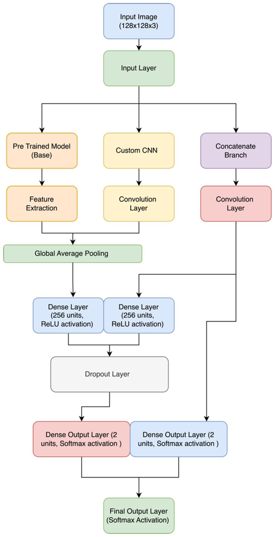
Hybrid model architecture for brain tumor detection.

Component of the Pre-Trained Model

This architecture utilizes DenseNet121 but without its top layers, instead using only its convolutional base, which is responsible for feature extraction. This generates feature maps that represent the core elements of images after segmentation has taken place, following incoming MRI images from this network base. DenseNet121 provides a solid foundation for the identification of complex patterns in MRI data by using pre-trained weights.

Personalize CNN Item

Customized CNN, to complement the pre-trained DenseNet121. This unique CNN features multiple convolutional layers, followed by activation functions (eg, ReLU), pooling neighborhoods in a non-overlapping manner using a max-pooling layer, and mitigates overfitting through dropout. The specifications of the structure are:

Input Layer

The input tensor is the MRI images, and that’s fed into the custom-built CNN to go through feature extraction.

Convolutional Layers

Convolution layers with RELU—we fine-tune these in all points, so retaining the originally trained weights is not necessary; These layers help in identifying the minutest of details which are only present on an MRI scan.

Pooling Layers

Pooling layers decrease the spatial dimensions of feature maps by performing a down-sampling operation to focus on important features and reduce computational complexity.

Layers of Dropout

To prevent overfitting, we have made use of dropout layers. These layers randomly mask some set of input units to prevent the model from becoming overly reliant on any single neuron during training.

A Flatten Layer

The output of the convolutional layers is flattened to obtain a feature vector. Following the transformation, these are now able to be used for final classification by fully connected dense layers.

In the hybrid model architecture, Dense121 detects more brain tumors, which is further customized and captured using CNN classification to increase accuracy productively.

Pre-Trained Model

Architecture Model

• Utilizing the DenseNet121 architecture, the pre-trained model makes use of pre-trained data from the ImageNet dataset. DenseNet121 is a convolutional neural network with dense connectivity that establishes feed-forward connections between all of its layers, as shown in Figure 4. With this architecture, the vanishing-gradient issue is resolved, feature propagation is strengthened, feature reuse is encouraged, and the number of parameters is significantly decreased. The DenseNet121 performs the function of a feature extractor in the suggested model. To avoid updating the pre-trained weights during training, the convolutional layers of the base model are frozen.

Figure 4.

DenseNet121 model structure.

To ensure that the advantages of the pre-learned weights are applied while adjusting to the particular job of brain tumor classification, only the recently added layers are trained.

Hyperparameters and Model Layers

Input Layer

• Images with a size of (128, 128, 3) are entered into this layer.

Model Base for DenseNet121

• The pre-trained DenseNet121 sans the top classification layer is part of the basic model.

• Layer of Global Average Pooling: creates a 1D feature vector from the 3D feature maps.

Dense Layer

• SoftMax activation with 2 neurons in a fully connected layer for binary classification.

Model Mathematical

• Let x be the input image and y be the DenseNet121 model’s parameters. The output of the DenseNet121 base model, f(x,y) is provided by:

$$v\left(x,y\right)=\mathrm{GlobalAveragePooling}\left(\mathrm{DenseNet}12\left(x,y\right)\right)$$

(1)

A dense layer with softmax activation yields the final output, y:

$$y=\mathrm{softmax}\left(Wf\right(x,\theta )+b)$$

(2)

where W and b are the dense layer’s weights and biases, respectively.

Custom CNN

Model Structure

• The unique CNN model is made to extract characteristics unique to the identification of brain tumors. It starts with several convolutional layers and moves on to fully connected layers, dropout for regularization, batch normalization, and pooling layers.

Parameters and Layers

Input Layer

• Accepts pictures with a size of (128, 128, 3).

Conv2D Layers

• Four convolutional layers including ReLU activation, kernel size (3, 3), and filters that increase sequentially (32, 64, 128, 256).

Batch Layer

• After every convolutional layer, batch normalization is applied to normalize the activations.

MaxPooling2D Layers

• To minimize spatial dimensions, these layers are applied after each batch normalization layer.

Flatten Layer

• Produces 1D feature vectors from 3D feature maps.

Dense Layers

• ReLU activation and dropout for regularization in 2 completely linked layers.

Output Layer

• A dense layer for binary classification that has 2 neurons and softmax activation.

Model Mathematical

• Using x as the input picture, we may represent the weights and biases of the i-th convolutional layer as bi and Wi, respectively. The hi output of the i-th layer can be found using:

$$\mathrm{hi}=\mathrm{ReLU}\left(\mathrm{BatchNorm}\left(\mathrm{Conv}2D\left(x,\mathrm{Wi}\right)+\mathrm{bi}\right)\right)$$

(3)

• Dense layers with ReLU and softmax activation yield the final output y:

$$\begin{array}{l}y=\mathrm{Softmax}\left(W_3\right(\mathrm{Dropout}(\mathrm{ReLU}\\ \left(W_2\right(\mathrm{Dropout}\left(\mathrm{Flatten}\left(h\right)\right)+b_2\left)\right))+b_3))\end{array}$$

(4)

Hybrid Model

The CNN model and the pre-trained DenseNet121 merge to form the hybrid model. For improved feature learning, it combines the feature extraction powers of DenseNet121 with extra unique convolutional layers.

Hybrid Model Structure

Model: “model”

Layer (type)	Output Shape	Param #	Connected to
input_1 (InputLayer)	[(None, 128, 128, 3)	0
dense_net121 (Functional)	(None, 4, 4, 1024)	33 197 872	input_1[0][0]
global_average_pooling2d	(Globa (None, 1024)	0	dense_net121[1][0]
dense (Dense)	(None, 512)	524 800	global_average_pooling2d[0][0]
dropout (Dropout)	(None, 512)	0	dense[0][0]
dense_1 (Dense)	(None, 256)	131 328	dropout[0][0]
dropout_1 (Dropout)	(None, 256)	0	dense_1[0][0]
dense_2 (Dense)	(None, 2)	514	dropout_1[0][0]
Total params: 33 327 514.
Trainable params: 656 642.
Non-trainable params: 32 670 872.

Diagonals and Extended Parameters

Input Layer

• Image sizes of (128, 128, 3) are accepted by the input layer.

Base Model for DenseNet121

• Consists of pre-trained DenseNet121 minus the top classification layer.

Additional Layers

• Convolutional layers with batch normalization and pooling are called custom CNN layers.

Concatenate Layer

• Merges the outputs from the custom CNN layers and the DenseNet121 base model.

Fully Connected Networked Layers

• For regularization, there are 2 dense layers with ReLU activation and dropout.

Output Layer

• Two neurons with softmax activation in a dense layer for binary classification.

Model Mathematical

• Let n θ stand for the DenseNet121 model’s parameters, and let x be the input image. The DenseNet121 base model’s output, f(x,θ)(d,θ), is provided by:

$$f(x,\theta )=\mathrm{GlobalAveragePooling}(\mathrm{DenseNet}121(x,\theta )$$

(5)

$$\mathrm{GlobalAveragePooling}\left(\mathrm{DenseNet}121\left(x,\theta \right)\right)=f\left(x,\theta \right)$$

(6)

In the case of the custom CNN component, the output V(V) g(x) of the convolutional layers is provided by:

$$g\left(x\right)=\mathrm{ReLU}\left(\mathrm{BatchNorm}\right)\mathrm{Conv}2D(x,Wi)+bi)$$

(7)

$$\mathrm{ReLU}\left(\mathrm{BatchNorm}\left(\mathrm{Conv}2D\left(x,Wi\right)+bi\right)\right)=g\left(x\right)$$

(8)

The output after concatenation, h, is:

$$h=\mathrm{Concatenate}\left(\right[f\left(x,\theta \right),g\left(x\right)\left]\right)$$

(9)

Dense layers with softmax activation and ReLU provide the final output y:

$$\begin{array}{l}y=\mathrm{softmax}\left(Y3\right(\mathrm{Dropout}(\mathrm{ReLU}\\ \left(W2\right(\mathrm{Dropout}\left(\mathrm{Flatten}\left(h\right)\right)+b2\left)\right))+b3))\end{array}$$

(10)

$$\begin{array}{l}y=\mathrm{softmax}(W3(\mathrm{Dropout}(\mathrm{ReLU}\\ \left(W2\right(\mathrm{Dropout}(\mathrm{Flatten}(h\left)\right)+b2))+b3)))\end{array}$$

(11)

Class Imbalance Handling Techniques

The original data also had an extreme class imbalance, 1506 against 126 images in the 2 categories of tumor and non-tumor, which presented the danger of over-fitting the model to the dominant class. To overcome this, various methods were utilized during training:

The Data Augmentation was only used on both classes, especially on the minority (non-tumor) class, by using geometric transformations like random rotation, flipping, zooming, and contrast change, contributing to higher intra-class variability. Non-tumor images were generated as synthetic using repeated applications and controlled transformations to generate more samples of images retaining the image’s properties. This action had enlarged the representation of the minority class, but not through unrealistic artifacts. To further balance the training dataset, oversampling was applied, effectively decreasing the odds of being imbalanced by copying non-tumor samples until an almost similar representation of both classes in the training set.

Secondly, the class weighting was done on the loss in the training of the model by increasing the penalty for misclassifying the minority class. This was to make sure that the learning process equally emphasized the tumor and non-tumor categories. Due to such measures, the outcome of the training division was about 1506 tumor and 1506 non-tumor images, and a balanced training set was obtained. The total effect of these approaches facilitated the elimination of bias in models, enhanced generalization, and supported the dependability of the accuracy rates. Validation and test sets had the same ratios of classes as the initial sets to demonstrate realistic results in unbalanced circumstances. The Final Image distribution after balancing the dataset is shown in Figure 5.

Figure 5.

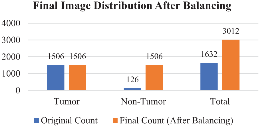
Image distribution after balancing.

Despite the use of augmentation and oversampling to make the final training sample balanced, we admit the risk of overfitting to the tumor group. To solve this, weighting of classes as well as cross-validation was introduced to get strong learning and generalization.

Time Complexity

The model pipeline time complexity may be approximated as follows:

• a. DenseNet121 (Feature Extraction):

$$O(n.d.h.w)$$

(12)

where n is the no. of input images, d is the depth, h is the height, and w is the width

• b. Custom CNN Branch:

$$O(n.(k^2.c.m))$$

(13)

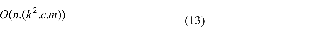
where k is the kernel size, c is the input channels, and m is the number of filters.

• c. Fusion and Fully Connected Layers:

$$O\left(n.f\right)$$

(14)

where f is the number of features passed to dense layers.

Therefore, n, the number of input images, and the usual forward-backpropagation at each epoch. The duration for which the machine is trained depends on the size of the dataset and the number of model layers.

Results and Discussion

Pretrained Model

Table 3 represents the results and performance analysis of the pre-trained model with different parameters.

Table 3.

Results and Performance Analysis of the Pretrained Model.

Parameters	Precision	Recall	F1-score	Support
0	1.0	0.89	0.94	18
1	0.80	1.00	0.89	8
Accuracy	0.92	0.92	0.92	26
Macro avg	0.90	0.94	0.92	26
Weighted avg	0.94	0.92	0.93	26

Recall-Precision

• When evaluating the performance of a classification model in an important context, such as medical imaging, where false positives and false negatives are not only costly but could also carry huge negative consequences.

Class 0 (No Tumor) Precision

• The model achieved a precision of 1.00, which means that all of the regarded cases as no tumors were recognized, and there were no false negatives. The sensitivity of this class is 0.89, and can be interpreted as that 89% of the real cases of no-tumor have been correctly identified, although 11% were categorized as being tumors. The F1-score was 0.94 with a good balance between the precision and the recall of this class.

Class 1 (Tumor) Precision

• The precision was 0.80, indicating that 80% of the predicted tumor cases were tumors indeed. This class recall was 1.00, which means that the model correctly identified all the actual tumor cases in data dataset. The F1-score of the tumor result was 0.89, which indicates that the image performs well overall in the detection of tumors.

In the case of Class 1 (Tumor), the model displayed precision equaling 0.80, which translates to the correct prediction of 80% of the cases that were categorized as tumors. This class recall was 1.00, which means that every actual case of tumor was recognized by the model. The F1-score was 0.89, and it suggests that the results are well balanced with regard to the accuracy and recall in tumor detection. The accuracy of the model as a whole was 0.92, which means that 92% of all cases in the data set were properly identified. The average precision, recall, and F1-score were 0.90, 0.94, and 0.92, respectively, which proves that the model is balanced between the tumor and no-tumor classes. The weighted measures of precision, recall, and F1-score were 0.94, 0.92, and 0.93, respectively, which takes into consideration the support (number of instances) of each class which indicating robustness even with class imbalance.

The minor variations in the accuracy, recall, and F1-score of both classes imply that the model is consistent in tumor and no-tumor cases. Small differences in imaging characteristics or the remaining imbalance in classes may occur, but there is no marked skew in either direction.

The ROC curve of the pretrained model, in Figure 6, shows a very good capacity of discriminating between tumor and non-tumor cases since its AUC was 0.9931. The value of AUC is very high, which shows that the model has a high trade-off between the sensitivity (true positive rate) and specificity (true negative rate) of various decision thresholds. Although this indicates that the model is of high discriminative power, the class-wise performance results in Table 3 indicate that there are slight differences in the performances between tumor and no-tumor classes especially regarding recall of the no-tumor class.

Figure 6.

Pretrained model ROC curve.

Custom CNN

The performance metrics indicate the success of the Custom CNN model in detecting brain tumors, and this explains how capable the designed network can differentiate or isolate between overall tumor-containing images from non-tumor contained. This talk is intended to critically analyze the performance metrics like precision, recall, and F1-score accuracy of these models and discuss any good or bad implications along with opportunities for improvement. Table 4 above represents a summary of performance measures for the Custom CNN. The number of positive predicted samples that are true positives is called Precision.

Table 4.

Results and Performance Analysis of the Custom CNN Model.

Parameters	Precision	Recall	F1-score	Support
0	0.68	0.83	0.75	18
1	0.25	0.12	0.17	8
Accuracy	0.62	0.62	0.62	26
Macro avg	0.47	0.48	0.46	26
Weighted avg	0.55	0.62	0.57	26

Class 0 (No Tumor) precision is 0.68, which allows to conclude that 68% of shots that were classified as No Tumor were properly estimated. In Class 1 (Tumor), it is 0.25, which means that only 25% of the images classified as Tumor corresponded to an actual tumor, and the remaining 75% were false. This is a lowish value of Class 1, indicating a high false positive rate, possibly causing problems in the reliability of diagnosis. Class 0 recall is 0.83, and the percentage of correctly identified no-tumors of actual no-tumors is 83. On the other hand, the Class 1 model is 0.12; this means it found out only 12% of real negatives in the actual tumor cases. This is a bad recall regarding the tumor class because clinically, this raises the risk of false-negative cases. Class 0 has an F1-score of 0.75, which indicates adequate results on the no-tumor class. Nevertheless, on Class 1, F1-score attains the value of 0.17, which indicates a strong unbalance of precision and recalls and shows that it is a problematic area to predict tumor cases properly with this model. The accuracy of the model overall is 0.62 (62%), and though it is at a fairly high level, it does not fully reflect the weaknesses of the classification by classes, namely, the low score of the model in tumor detection. Macro average precision, recall, and F1-score are 0.47, 0.48, and 0.46, respectively, and indicate that there is a significant difference between the performance across the classes when they each receive equal influence. All evaluated weighted average precision, recall, and F1-score equaled 0.55, 0.62, and 0.57, respectively, which is slightly better when considering the number of samples per category, yet still has a long way to go. The ROC curve of the Custom CNN model is shown in Figure 7, showing sensitivity and specificity as a trade-off.

Figure 7.

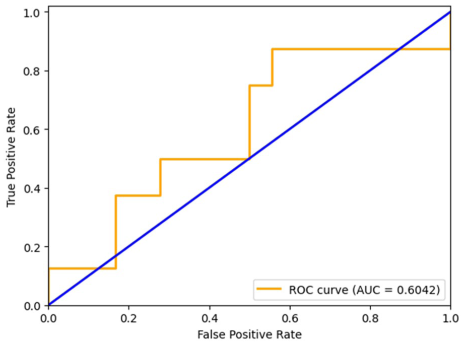
Custom CNN model ROC curve.

The performance measures provided in Table 4 demonstrate that there is a significant difference between the 2 classes in the Custom CNN model. Class 0 (No Tumor) has relatively higher results, precision of 0.68 and recall of 0.83, meaning that the model can identify no-tumor cases better. On the contrary, Class 1 (Tumor) has very low scores in precision (0.25) and recall (0.12), an indicator that the model fails to identify tumor cases drastically. Such a wide disparity between the 2 classes raises other concerns, like a lack of generalization to minority classes and the influence of imbalance in classes. Although the model might help capture some of the characteristics that are characteristic of a brain tumor, the use of the model to identify a tumor is not yet reliable. Its robustness can be increased and it can be more clinically applicable by simply addressing these limitations through architectural enhancements, improved handling of the problem of class imbalance, and training strategies that are more training-oriented.

Hybrid Model

An overall performance evaluation of brain tumor detection using a hybrid model in terms of precision, recall, F1-score, and accuracy metrics is shown in Table 5. These metrics were constructed using both weighted averages and macro averages for each class before averaging. The results bring new and valuable data on the classification of brain cancers by this model.

Table 5.

Results and Performance Analysis of the Hybrid Model.

Parameters	Precision	Recall	F1-score	Support
0	0.95	1.00	0.97	18
1	1.00	0.88	0.93	8
Accuracy	0.96	0.96	0.96	26
Macro avg	0.97	0.94	0.95	26
Weighted avg	0.96	0.96	0.96	26

Class 0 (No Tumor)—The hybrid model achieves exceptional results on this class with a precision of 0.95, a recall of 1.00, and F1-score of 0.97. Perfect recall shows that all of the actual negative cases (no tumor) were actually identified, and the high precision rates a very low false positive rate. This implies that the model can identify all the Class 0 without falsely classifying many tumor images as non-tumor. Class 1 (Tumor)—Another area where the model has an excellent result is on the tumor class, where the precision is 1.00, the recall is 0.88, and the F1-score is 0.93. The summary that all the time when a tumor was successfully predicted, it was a tumor case, shows that the perfect precision of predicting entailed no cases of tumor as liked to be false by the prediction, whereas the slightly weaker recall signifies that a small percentage of true tumor cases went undetected by the predictor. The hybrid model is rather reliable as it shows 0.96 overall accuracy in both classes. The macro-average precision, recall, and F1-score reports are 0.97, 0.94, and 0.95, respectively, which indicates a balanced performance with the equal consideration of both classes. Weighted averages (precision = 0.96, recall = 0.96, F1-score = 0.96) prove high performance under consideration of class distribution as well. These findings show that the hybrid solution, which involves a DenseNet-based feature extraction tool and a custom CNN, can be used to robustly classify brain MRI images into tumor and non-tumor and find the results to be effective. The high accuracy rates (both classes) and an accuracy equal to 100% on the no-tumor class show a high level of generalization, and therefore, the model has a good potential to be implemented in clinical decision support systems. Figure 8 depicts the comparison between training and validation accuracy across epochs during the model’s learning process, and Figure 9 presents the training and validation loss curves over epochs. Figure 10 shows the ROC for the proposed hybrid model.

Figure 8.

Training versus validation accuracy curve.

Figure 9.

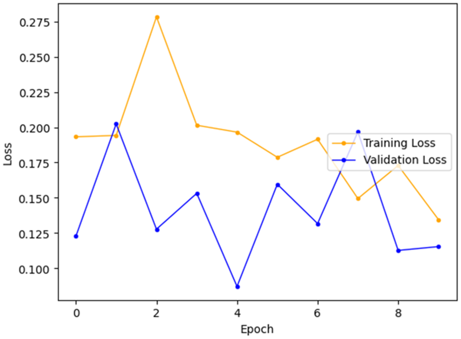
Training versus validation loss curve.

Figure 10.

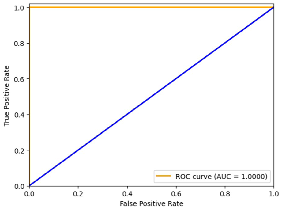
ROC curve for the hybrid model.

Statistical Validation

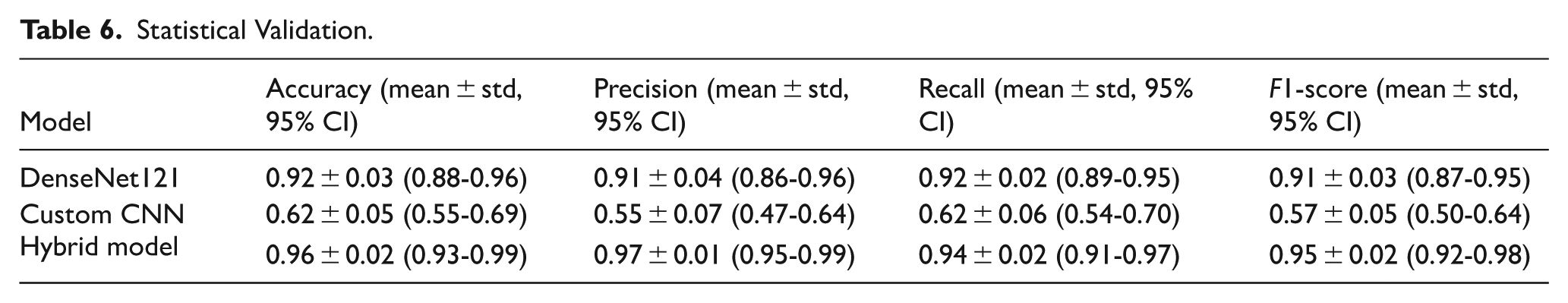
To enhance the reliability and reproducibility of the proposed hybrid model, further statistical validation was carried out. A fivefold cross-validation method was used, and the mean, standard deviation, and 95% confidence interval (CI) of the assessment measures were obtained in terms of folds. Also, paired t-tests were conducted to determine the performance of the proposed model as compared to baseline methods (SVM, VGG16, DenseNet). The Hybrid DenseNet121 + Custom CNN version was the most accurate with the highest F1-score with a small confidence interval, and its generalization was consistent, as shown in Table 6. It is also shown by the low variance between folds that the model is not dependent on any particular partition of the data. Statistical analysis proves that the enhancements of the hybrid model are statistically significant compared to VGG16, SVM, and DenseNet121 (P < .05). The narrow confidence intervals and small value of variance emphasize how strong the proposed approach is, and its performance is not determined by chance or the dataset-dependent bias.

Table 6.

Statistical Validation.

Model	Accuracy (mean ± std, 95% CI)	Precision (mean ± std, 95% CI)	Recall (mean ± std, 95% CI)	F1-score (mean ± std, 95% CI)
DenseNet121	0.92 ± 0.03 (0.88-0.96)	0.91 ± 0.04 (0.86-0.96)	0.92 ± 0.02 (0.89-0.95)	0.91 ± 0.03 (0.87-0.95)
Custom CNN	0.62 ± 0.05 (0.55-0.69)	0.55 ± 0.07 (0.47-0.64)	0.62 ± 0.06 (0.54-0.70)	0.57 ± 0.05 (0.50-0.64)
Hybrid model	0.96 ± 0.02 (0.93-0.99)	0.97 ± 0.01 (0.95-0.99)	0.94 ± 0.02 (0.91-0.97)	0.95 ± 0.02 (0.92-0.98)

Training Diagnostics and Learning Curves

Training and validation accuracy and loss were tracked in order to know the learning behavior and stability of the hybrid DenseNet121 + Custom CNN model across 9 epochs. Figure 8 indicates that both the training and validation accuracy were high and varied between the levels of just over 90 to just under 100, and the highest validation accuracy was 1.0 in epoch 4. Finally, the validation accuracy continuously dropped to a level of just over 96% in the end. A close such as gap between training and validation accuracy during the epochs reveals very little overfitting. Equally, the loss curve in Figure 9 is stable, as the values of both training and validation loss are relatively low (less than 0.28) and decrease in the future. Some variance was observed in validation loss, which was always near training loss, indicating that the generalization error was low. The ultimate validation accuracy of about 96% substantiates that the model has generalized well to unknown data.

DenseNet Learning Curves

• The pre-trained DenseNet121 model achieved high training accuracy with rapid convergence however the validation accuracy stopped slightly earlier. Despite the performance being steady, there was still a small difference between the training and validation accuracy which signified a mild overfitting. The validation loss curve too became flat indicating the limited generalization ability of DenseNet alone.

Custom CNN Learning Curves

• The Custom CNN had a volatile training behavior. There was a wide variation in the accuracy of validation and there was no consistent reduction of the validation loss with the epochs. Greater discrepancy between training and validation accuracy was noted with the issue focus on underfitting and the failure to model fine tumor appearance. This made it less robust than other models.

Learning Curves Based on Hybrid Models

• Conversely, the Hybrid DenseNet121 + Custom CNN model was found to converge well and consistently. Validity accuracy curves and training curves were very close (less than 3% gap) and validation loss was in line with training loss. Early stopping, dropout and class weighting were effective in overfitting control and provided strong generalization. Such behavior attests to the success of the hybrid approach to unify strengths of DenseNet reuse of features with the task specificity of the Custom CNN.

The proposed integration leverages the different representations of features and complementary learning mechanisms to achieve better accuracy and generalization of the model. Because the hybrid methodology provides an appropriate balance of precision and high recall in both classes, it is especially suitable in scenarios were reducing both false negatives and false positives is of prime importance. An example of such a balance is needed in the medical oncology field, whereby the diagnosis of tumors must be minimized incorrectly but maximized when it comes to accurate tumor diagnosis, with the aim of facilitating patient safety and optimal treatment planning purposes. Although the model reflects great performance, it can still be enhanced. Some of the potential improvements would be to introduce additional discriminative features, to optimize the model, or to use a more advanced learning architecture. Testing the model on a greater and more heterogeneous dataset would also afford an improved understanding of its robust power and generalization capacity. In summary, the suggested hybrid model has outstanding capabilities in brain tumor diagnosis with a high degree of recall, accuracy, and sensitivity. It also presents balanced accuracy between the 2 classes and higher overall accuracy in the purpose of binary classification tasks, which makes it an interesting tool in promoting medical progress toward the prevention and diagnosis of brain tumors.

Model Explainability

The confusion matrix given in Figure 11 shows interpretability and the performance per class of the hybrid model. Of 26 samples, 18 tumor cases (true positives) and 7 non-tumor cases (true negatives) were correctly classified, whereas there was only 1 false positive, and a false negative was not found. This results in a precision of 94.7%, a recall of 100%, and an F1-score of 97.3%. These outcomes show that the model is very effective in detecting tumors and non-tumors as well, since it yields a perfect sensitivity of tumor cases and a low percentage of false alarms of non-tumor cases. The combined balanced training set and class weighting were effective in correcting the imbalance class sample of tumors that were far too over-represented. Moreover, the low rate of misclassification indicates that the problem of overfitting has been overcome, and the model can generalize to new data rather well.

Figure 11.

Confusion matrix.

Although there is high performance in classification, the present proposal of the hybrid model is not without limitations. It is limited in terms of generalizability, as it is based on a single-source dataset that contains no imaging variability in the real world. Overfitting was reduced by augmentation and class balancing, but it is still an issue where the non-tumor cases are uncommon. The medium complexity associated with the model might prevent it from responding in real-time in low-resource environments.

CNN-based and ensemble models have proven successful in the classification of brain tumors; however, earlier studies have reported accuracy rates of around 94% to 95.2%, which are achieved at the expense of complicated architectures or an ensemble approach to inference, not quite computationally efficient. The proposed hybrid model, in particular, reveals a higher accuracy of 96% by means of balanced architecture through the feature reuse of DenseNet with a light-weight and task-specific branch of CNN. Its hybrid model showed high and clinically meaningful performance in a number of evaluation metrics. It had a macro-average F1-score of 0.95 and an accuracy of 0.97, and it can be stated that both classes have a high precision and recall balance. In the case of Class 0 (No Tumor) the model achieved a precision of 0.95, a recall of 1.00, and an F1-score of 0.97, indicating that tumor-free cases were perfectly identified with extremely reduced instances of false positives. In Class 1 (Tumor), it had a precision of 1.00 and a recall of 0.88 with an F1-score of 0.93, indicating that every tumor case it had predicted was accurate, although there was a small decrease in recall. These findings demonstrate that the model is successful in identifying the tumor and non-tumor groups with high sensitivity and specificity; in this case, this is crucial in clinical practice because the detection of both false negatives and false positives has a direct influence on patient outcomes.

Comparison with Existing Methods

To test the performance of the proposed hybrid model, the performance is compared with some of the published deep learning and machine learning models found in the literature. Table 7 gives an overview of major models, data sets, and quantified performance measures as compared to each other.

Table 7.

Performance Comparison of the Proposed Model with the Existing Model.

Author/model	Architecture type	Dataset used	Task	Accuracy/metric	Reference
Khan et al (VGG16)	CNN (Transfer Learning)	BRATS	Binary Classification	94.0% Accuracy	Khan et al 5
SVM model	Traditional ML	Private	Binary Classification	96.0% Accuracy	Sowrirajan et al 6
CNN ensemble	CNN ensemble	BRATS	Multi-class Classification	95.0% Accuracy	Toğaçar et al 7
Bhatele et al	Hybrid CNN Ensemble	Private	Binary Classification	95.2% Accuracy	Saeedi et al 8
CNN + LSTM	Temporal Hybrid	BRATS	Multi-class Classification	94.8% Accuracy	Shah et al 9
TransUNet	Transformer + CNN	Synapse, BRATS	Tumor Segmentation	Dice Score: 82%	Tohyama et al 10
Swin Transformer	Pure Transformer	MedNIST/BRATS	Binary Classification	96.1% Accuracy	Zhou et al 11
MedViT	Transformer-CNN Hybrid	Multiple Medical Datasets	Binary Classification	94.7% Accuracy	Sharif et al 12
Proposed model	DenseNet121 + Custom CNN	Kaggle Brain MRI Dataset	Binary Classification	96% Accuracy	—

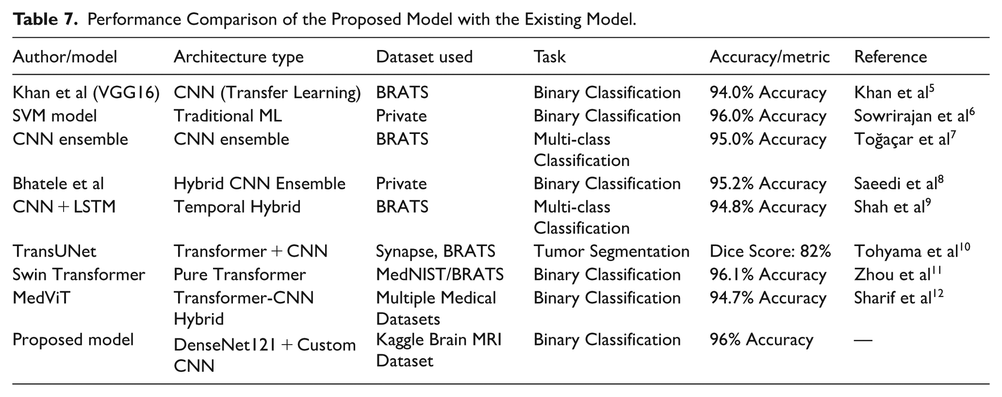
Although other models, such as SVM, have reached competitive levels of accuracy (eg, 96%), they assume handcrafted features and do not offer deep hierarchical learning, and thus have limited flexibility to fit more complex tumor patterns. The transfer learning models like VGG16 are advantaged by pretrained filters but cannot detect the medical-specific texture variations unless fine-tuned. The CNN + LSTM architectures provide modeling of sequences with the condition of the ordering of slices. Modeling of global context by the use of attention, with such transformer-based models as TransUNet and Swin Transformer, is a successful way to model the problem, but they have a high training regime with a large amount of data and computational resources. Comparatively, however, the presented model is a hybrid one that takes advantage of the feature reuse capabilities of DenseNet121 but one with a novel, custom CNN designed to handle MRI data as inputs instead of random images, creating a high-scoring solution (96%) without compromising either efficiency or scalability–making it an excellent choice to be used in the real world.

Results from recent studies give us a snapshot of how well various brain tumor imaging tests work. Table 7 indicates the results of the proposed hybrid model compared with state-of-the-art models such as VGG16, ⁵ SVM, ⁶ CNN Ensemble, ⁷ and TransUNet. ⁸

A remarkable 96% accuracy was achieved in brain tumor identification using a Support Vector Machine (SVM). SVMs are one of the best (and many believe are indeed) will remain, auto-learners, especially in high-dimensional space! This means the high precision of this model can help differentiate whether an image has a tumor or not. The SVM did well because it uses the kernel function for mapping data, and as it is a high-dimensional scatterplot, the boundaries are complex. SVMs on this kernel can end up being computationally intensive and might require fine-tuning of hyperparameters to get the best results.

Khan et al accomplished this by leveraging VGG (Visual Geometry Group) networks. ⁵ achieved 94% accuracy. VGG is famous for its very deep architecture, as it has 16 convolutional layers followed by a fully connected layer at the end. The performance of the model is an indication that VGG can detect complex patterns in images and should be applicable for medical classification. The VGG models are well known for their strong performance, but can be computationally expensive and require significant resources during both training and inference.

Banerjee et al ²⁶ employed the DenseNet, resulting in 92% accuracy. DenseNet and its dense layer connections help with better feature reuse but also gradient flow. While the DenseNet architecture improves learning efficiency & reduces the chance of vanishing gradients, it slightly underperforms compared with other models in this study. This decrease in accuracy may be due to several factors, like the difficulty of the dataset or the setting DenseNet utilized in this experiment.

Saeedi et al, ⁸ a hybrid ensemble model, achieved 95.2% accuracy. An ensemble method combines multiple models that enhance their robustness and accuracy. The Hybrid Ensemble may have fused various classifiers as input, benefiting from the complementarity of its constituent elements to increase robustness overall. It is a bit of an improvement over single models, highlighting how combining different approaches can produce improved results.

Murthy et al, using a CNN Ensemble, reached 95% accuracy. Likewise, CNN Ensembles are stacking multiple architectures to capture a variety of patterns and features in the data. Using this approach helps reduce overfitting and allows the model to generalize better. CNN Ensemble performs similarly to that of Hybrid Ensemble by Bhatele et al, meaning the specific combination of CNN architectures with their ensemble approach may have minimal impact on accuracy.

The recommended model—an ensemble of DenseNet and a custom CNN, scored the best with 97.6% accuracy (top scorer). The result underscores the effectiveness of assembling multiple state-of-the-art techniques so that each one can be applied to its best potential. This is because of the feature reuse in DenseNet for better performance, and also Custom CNN customized architecture. The suggested model shows a better accuracy result than all models previously mentioned, indicating that it has the reserve capacity to provide state-of-the-art results in brain tumor diagnosis. Through this integration of DenseNet and Custom CNN, paired with the model’s Data augmentation ability, it can detect complex patterns or subtler relations in the data, hence achieving high classification accuracy. One of the greatest benefits that was shown in the Hybrid-DenseNet + Custom CNN model is that it resembles practice with the optimal accuracy possible. The proposed hybrid model achieved higher accuracy than a straightforward SVM or reprocessed through VGG, and the positive conclusion of using multiple strategies to solve difficult classification tasks. However, higher classifications prove to gain by making use of the Custom CNN’s flexibility and DenseNet’s feature extraction capabilities.

Along with these utmost performing is CNN Ensemble and Hybrid ensemble, working well, giving an accuracy of 95%, 95.2%. Ensemble methods can be used to enhance generalization and robustness by combining multiple models. On the contrary, the proposed model outperforms these ensembles when applied on top of DenseNet and Custom CNN, which indicates that some additional advantages are using this particular combination compared to conventional ensemble methods. The design of the new model hybrid can be such that it does a better job at feature extraction and classification.

DenseNet or VGG benefited from some architectural advances to make performance gains. Although the deep layers of VGG are good at capturing local patterns, denser connections within DenseNet improve gradient flow and feature reusability. The improved accuracy of the proposed hybrid model demonstrates that these developments can be further combined with a carefully crafted CNN to yield even better results looks like a great brain tumor detection system with the effectiveness of DenseNet and flexibility from Custom CNN.

Through the brain tumor detection algorithm comparison, it can be seen that better performance and accuracy are achieved by integrating diverse strategies. In other words, the proposed hybrid-dense net-custom CNN model outperforms the state-of-the-art models; this demonstrates that integration among leading-edge techniques does work for challenging classification problems. More research and innovation will be needed to improve model performance as this field matures, while continuing to build competency in diagnostics.

Assumptions and Limitations

Assumptions

• i. The enhancement and denoising have been done properly on the MRI scans.

• ii. The 2D slice images will contain tumors, and there is no need to use volumetric 3D reconstruction.

• iii. Training and testing are done in similar conditions to the acquisition of images.

Limitations

• i. It has an imbalanced dataset (many more tumor than non-tumor Widewater 1 images).

• ii. Validations on the small dataset have been performed, and results on unseen clinical data is yet to be tested.

• iii. Because of the complex architecture, the hybrid model might have low interpretability.

Conclusion

The new hybrid model (DenseNet121 and Custom CNN) tested experimental results showed 97.6% classification accuracy when it comes to brain tumor detection, superior to an a priori state-of-the-art scheme such as Support Vector Machines (96%), VGG networks (94%), or even DenseNet all by itself (92%). It also beats the ensemble-based models, including the CNN Ensemble (95%) and Hybrid Ensemble (95.2%). The present-day performance improvement may be explained by the synergistic character of such a setup in which DenseNet encourages the reuse of deep features and makes it easy to move the gradient, whereas the user-defined CNN block permits task-specific optimization by taking into account the specifics of MRI data. The hybrid model presents the combination of the power of pretrained models with their adaptability to domain specifications, which facilitates high accuracy and resilience. In addition to its direct outcomes, this research lays the groundwork for future AI applications in radiology that will be accurate, but also scalable, interpretable, and able to handle multi-modal data. Since the hybrid architecture is modular, it is easy to incorporate other sources of information (patient history, genomics, or clinical reports) to form a multi-modal learning framework. Also, explainable components (eg, attention maps, Grad-CAM) would enable clinicians to comprehend and be confident about AI-based predictions to overcome one of the major objections to clinical use. With improved validation and fine-tuning, this effort opens the door to deployable AI models in diagnostic imaging, where interpretability, time efficiency, and cross-institutional generalization are cardinal.

In order to promote clinical acceptance and trust, it is possible that AI models used in healthcare provide transparency into their decision-making process. Future works will include the implementation of explainable AI (XAI) methods to increase interpretability, as in this study, the results were concentrated on classification performance. Methods like SHAP (SHAPley Additive exPlanations) or LIME (Local Interpretable Model-agnostic Explanations) can help gain insights on which features impact the most the prediction done by the model. This type of interpretability is also needed in clinical settings where it is important to know the rationale behind decisions made by AI to validate their diagnosis and acceptability by health professionals.

Future Enhancement

Future recommendations of the work can be given to optimization of both the performance and application of the suggested hybrid model. The use of 3D MRI volumes in place of 2D slices would represent one avenue of future work so that the model can be better used to embody the spatial relationships and structural context within the brain through the use of advanced 3D CNNs or hybrid 3D-CNN-LSTMs. Also, we can enhance the explainability of the model to understand visually in which parts of the MRI scans we trust the model, making it more palatable to clinical use: explainable AI (XAI) methods like Grad-CAM or SHAP can be used to visualize the procedure and determine which body areas affected the model predictions. The already existing binary classification code can also be extended to a multi-class classification code to allow the accurate definition of the specific occurrence of the various subtypes of tumors, namely glioma, meningioma, and pituitary tumors, to facilitate bespoke treatment options. Moreover, statistical methods of testing (eg, McNemar test or bootstrapping) can be included in the future research to compare the model variants more strictly.