Sage Journals: Discover world-class research

Abstract

Background:

The adoption of electric vehicles for mobility is seen as a major step towards the conservation of the environment. In India, slow-moving Electric 3-Wheelers (E3Ws) have been adopted for last-mile connectivity. The present study investigated the impact of slow-moving electric 3-wheelers on the environment in terms of emissions and traffic performance in mixed conditions.

Methods:

Field traffic data from a section of road in the city of Lucknow was collected and used for the calibration of the traffic model. A total of 6 scenarios were tested using traffic modelling in the open-source microsimulation software SUMO. Krauss model was used to model mixed traffic and HBEFA 4 was used to calculate the emissions of fuel-driven vehicles. In each scenario, the volume of fuel-driven vehicles was kept constant and the volume of E3Ws was varied. For the last 2 scenarios, E3Ws were replaced with modified Electric 3-wheelers (ME3Ws) and Electric Buses.

Results:

Initial findings showed that the average emission decreased as the number of slowly moving electric vehicles increased, but the average flow and harmonic mean speed decreased by 49.8% and 28.8%, respectively, despite keeping the original composition of fuel-driven vehicles the same in every scenario. Further analysis of scenarios revealed a strong correlation ( $R^{2} = 0.88$ ) between the reduction in the number of vehicles and the reduction in emissions like Carbon Dioxide ( ${CO}_{2}$ ), which is responsible for global warming. Scenarios in which faster electric vehicles and electric buses replace slow-moving E3Ws also demonstrate emission reduction without noticeably affecting traffic performance parameters.

Conclusion:

The study shows that the environmental benefits of E3Ws in a limited section of Lucknow road are offset by their low-speed capability. Hypothetical scenarios wherein Modified E3Ws and Electric Buses were introduced reported benefits both in terms of emissions and traffic performance.

Keywords

Emissions electric three wheelers traffic microsimulation pollution

Introduction

Pollution is a major contributor to the dangers posed to both human health and the natural state of the environment.¹ About 1.2 million people per year die as a direct result of exposure to environmental pollution.² This is exacerbated by the use of automobiles, which are generally accepted as single largest contributor to air pollution³ and it has necessitated a push to decrease vehicular pollution.⁴ Emissions from automobiles have emerged as a major concern in recent years⁵ and rising number of automobiles on roads has made the situation grimmer.⁶ Also, the evolution of traffic flow, traffic speed and traffic density play important roles in air pollution.⁷ Emissions of carbon monoxide (CO), nitrogen oxides ( ${NO}_{x}$ ), Total HydroCarbons (THC), particulate matter ( ${PM}_{x}$ ) and greenhouse gases like Carbon Dioxide ( ${CO}_{2}$ ) are the primary constituents of vehicle exhaust.⁸

Introduction of electric vehicles is seen as a major step in reducing air pollution as well as noise pollution.⁹ Requia et al¹⁰ in their review concluded that the introduction of electric vehicles resulted in a reduction in emissions, particularly PM and SO₂. Authors reported that almost all studies show a reduction in emissions but attribute the reduction to several factors which include the type of electric vehicle. In India, a similar trend has been seen but the type of electric vehicle adopted in India for public transport is not the same as seen in developed economies. The present study aims to study the impact of slow-moving Electric 3-Wheelers (E3Ws) on sections with weaving traffic. The study investigates whether the low-speed capabilities of E3Ws negatively impact traffic performance. In the last decades, it has been observed that the population of E3Ws, also known as e-rickshaws, has increased rapidly.¹¹ This is due to factors like affordable cost, low maintenance, low operating margin and ease of driving on narrow urban roads.¹² They have medium to low-speed capability and are designed to replace manual pulling rickshaws. The presence of these E3Ws was limited to the sub-urban area only and not on the major city roads¹³ but this trend has been changing.

Background

To reduce the pollution due to vehicles, electric vehicles are being introduced in cities.¹⁴ Electric vehicles reduce the emission of greenhouse gases such as carbon dioxide (major), nitrous oxide and methane (minor) in the environment of the city and address the issue of global warming.¹⁵ Twenty-five percent of PM and one-third of India’s PM pollution are caused by the transportation industry with a rise in levels of ${PM}_{2.5}$ in Indian towns.¹⁶ Recently, world leaders have agreed (Paris Climate Agreement) to move towards achieving a net zero level of carbon emissions in the future.¹⁷ One of the major steps towards this goal will be replacing fuel-driven vehicles with electric vehicles.¹⁸ Electric vehicles have multiple advantages, such as zero emissions, simplicity, reliability, cost efficiency, comfort, efficiency and accessibility. Over the past 5 years, E3Ws have been used in Lucknow’s public transportation system. For vehicle propulsion, these vehicles use brushless DC motors that are powered by traditional lead-acid batteries.¹⁹ Since they transport passengers, e-rickshaws are environmentally benign and have the potential to lower carbon emissions.²⁰ The main concern with these E3Ws is that they were not permitted to be used as a form of public transportation.²¹ Technical issues persist such as the need to meet safety requirements in the production and design of the E3Ws, which are assembled in poorly equipped factories. Moreover, their slow speed at the traffic junctions causes congestion in the city and slows down the movement of other vehicles. Since e-rickshaws were not even covered by the Motor Vehicles Act of 1988, it was impossible to legalize them as a form of public transportation. To guarantee the legalization of these vehicles, the Indian government passed additional modifications in December 2014, during the most recent legislative session.¹⁹

Methodology

The objective of this study is to study the impact of slow-moving E3Ws on overall emissions and traffic performance in mixed conditions. In this study, a busy road section of 170 m is considered for investigating the potential impacts of E3Ws. The study aims to present findings from a preliminary investigation of a small section with merging traffic from high-speed National Highways and traffic from local arterial roads in a simulated environment using SUMO. The Traffic Data for the simulation model is collected from an elevated overpass and extraction of traffic volume (vehicles per hour) and speed (kilometre per hour) is done using a semi-automatic Traffic Data Extractor²² developed by Transportation Systems Engineering, Department of Civil Engineering Indian Institute of Technology, Bombay. For the simulation model, the network is developed by importing an open street map file of the study area and converting it to a .net file using the netconvert Python script. The simulation model parameters are defined and are explained in the section Mixed Traffic Modelling. The methodology for this study is shown in Figure 1. A total of 6 scenarios are developed to understand the impact of the E3Ws on the environment. A similar approach for scenario development has been used by Lertworawanich and Unhasut²³ for CO emission study as well as by Chandra et al (2016)²⁴ for highway capacity study. For scenario 0, the E3Ws are removed completely from the traffic stream. Scenario 1 represents the actual field conditions with 9.9% E3Ws. For scenario 2 and scenario 3, the percentage of E3Ws is taken as 19.8% and 29.7% respectively. In scenario 2 and scenario 3 the percentage of E3Ws is doubled and tripled respectively to capture the future traffic composition especially due to the exponential growth of slow-moving E3Ws which has a negative impact on traffic speed as platooning by slow-moving E3Ws can lead to substantial speed drops in traffic stream²⁵ In scenario 4, E3Ws were replaced by Modified Electric Three-Wheelers (ME3Ws) which have powerful motors and have a higher maximum speed comparable to cars. Lastly, for scenario 5 all E3Ws are replaced by electric buses, and their volume is adjusted as per the passenger carrying capacity of the E3Ws. Scenario 4 represents any intervention of policymakers to amend the minimum power requirement of electric vehicles before granting commercial operation licences. Scenario 5 represents the possible electrification of the bus fleet due to their advantages over fossil fuel-powered buses.²⁶ Mean traffic flow and mean harmonic speed of the traffic stream were considered measures of effectiveness in terms of mobility. The average emission per unit of time was considered a measure of effectiveness in terms of environmental impact. In the next section study area is explained followed by the mixed traffic modelling wherein the traffic model used and vehicle characteristics are explained. It is followed by model calibration and validation. The emission model is discussed in the next section. The penultimate section presents the findings of the study and in the last section conclusions are presented.

Figure 1.

Flow chart showing the methodology of the study.

Study Area

Lucknow is the capital city of the state of Uttar Pradesh, which has the largest population among all states in India.²⁷ It is also one of the fastest-growing cities in India. There are many public transportation modes available in the city, such as the metro, city bus, autorickshaw, electric 3-wheelers, 2-wheelers, etc.²⁸ The road section taken for this study is a 170 m two-lane road which widens to 4 lanes, with a maximum width of 14.5 m, before meeting an intersection. The road is the connection between the National Highway, connecting the regional capital city Lucknow with the national capital city New Delhi, and the ring road in Lucknow. There is an on-ramp joining an arterial road with the main road. The criteria used to select the section was the weaving of traffic due to an on-ramp,²⁹ a continuous undisturbed section with 4 possible exit routes which results in mixed traffic and lane-changing manoeuvres. This mixing of fast-moving traffic with slow-moving E3Ws leads to decreased speed for fuel-driven vehicles. Due to the presence of educational institutes, hospitals, commercial outlets and residential areas, there is a substantial presence of slow-moving E3Ws. This creates a situation of merging traffic streams, especially during evening peak hours and is the worst-case scenario for this road. Traffic data was collected at the 4-lane stretch from 17:30 to 18:30 hours on weekdays by installing a camera at a pedestrian overpass. The classwise traffic flow and speed values were extracted using the Traffic Data Extractor (IIT Bombay). The percentage of 2-wheelers was found to be 56.61%, and for cars, it was 25.81%. The percentage of Light Commercial Vehicles (LCV) and buses was 6.6% and 1%, respectively. The percentage of E3Ws stood at 9.9%. The network model was developed by importing the open street map of the study road section. The osm file from the open street map was converted to a network file using the netconvert module of SUMO using the command netconvert-osmfilesmap.som-test.net.xml on the command prompt. The plan of the study area and the corresponding network file are shown in Figure 2.

Figure 2.

Aerial view of the study area and modelled network file in SUMO.

Mixed Traffic Modelling

Simulation of Urban MObility (SUMO), developed by German Aerospace is an open-source microscopic traffic simulation software used to model and simulate traffic behaviour in urban areas. It is a widely used tool in transportation research, urban planning and traffic management. It is highly portable and can be used to create detailed models of road networks, simulate the movement of vehicles and pedestrians, and analyse various aspects of traffic flow and congestion. Mixed traffic here refers to a composition of traffic where heterogeneity exists in dimension as well as speed characteristics. Figure 3 shows the lack of lane discipline and the presence of E3Ws in the traffic stream. Munigety and Mathew³⁰ discussed the suitability of traffic modelling approaches for mixed traffic conditions. For car following, they found that collision avoidance approaches were best suited for mixed traffic conditions. The car-following model considered for the study is the Krauss model as it satisfies the criteria for a collision-free car-following model.³¹ The Krauss model was proposed by Stefan Krauss and is a stochastic version of the Gibbs model. It belongs to the category of models which are based on ‘safe distance’. The safe speed $V_{s}$ is calculated as follows:

V_{s} = v_{l} (t) + \frac{g_{n} (t) - v_{t} (t) T}{(\frac{v_{f} (t) + v_{l} (t)}{2 b}) + T}

(1)

Where $v_{l} (t)$ is the speed of the leader vehicle at time t, $g_{n} (t)$ is the spacing between the leader and follower vehicle at time t, $v_{f} (t)$ is the speed of the follower vehicle at time t, $b$ is the maximum deceleration and $T$ is reaction time. Equation (1) gives a speed which can be too conservative therefore desired speed $v_{d e s i r e d}$ is calculated as:

v_{d e s i r e d} = M i n (v_{f} (t) + a t, v_{s a f e}, v_{l i m i t})

(2)

Where $a$ is acceleration, $t$ is time and $v_{l i m i t}$ is the maximum speed capability of the vehicle. Equation (2) satisfies the safety, legal and vehicle-linked constraints. To add randomness in driver behaviour and thus achieve variation in speeds of drivers two terms for noise amplitude (∈) and a random number ( $η$ ) are added for the calculation of speed as shown in equation (3).

v_{t + T}^{f} = \max (0, v_{d e s i r e d} - \in a η)

(3)

Figure 3.

Snap from the traffic recording showing the use of sub lane and presence of E3Ws.

The Maximum Speed ( $v_{l i m i t}$ ) refers to the absolute physical speed limit or capability of a vehicle in perfect conditions, in which traffic flow, congestion, or driver behaviour are not taken into consideration in any way. It is a value that is often unchangeable and indicates the maximum speed that a vehicle is capable of reaching due to the combination of its design and its power. On the other hand, the driver’s or driving population’s preferred or desired speed in the presence of traffic and other conditions is represented by the maximum desired speed. It is frequently impacted by a variety of factors, including drivers’ attitudes, the amount of traffic on the road, traffic density and road conditions. The maximum desired speed is generally lower than the maximum speed. Since the considered study section is only 170 m boundary conditions need to be defined for exit and entry of vehicles. The parameter departlane³² is set to ‘free’ and departspeed is set to ‘desired’ for entry of vehicles mimicking the field conditions as vehicles entering the 170 m length have no external disturbance due to the preceding grade-separated section. A similar approach is adopted for vehicles entering via the on-ramp. For exiting the section, vehicles have 4 major and 2 minor roads. Since the congestion at the intersection is beyond the scope of this study it is assumed that vehicles exit by slowing down and moving to the desired road.

For the lane change model, SL2015 is used which is an advanced version of LC2013 which in turn is based on MOBIL (Minimizing Overall Braking Induced by Lane Change) proposed by Triber. The equation is given by:

{\hat{a}}_{α} - a_{α} + p ({\hat{a}}_{\hat{f}} - a_{\hat{f}} + {\hat{a}}_{f}) > Δ a + a_{b i a s}

(4)

Where ${\hat{a}}_{α}$ is the acceleration function of the leader vehicle after lane change, $a_{α}$ is the acceleration function of the leader vehicle before lane change, ${\hat{a}}_{\hat{f}}$ is the acceleration function of a new follower after lane change, $a_{\hat{f}}$ is the acceleration function of the follower, ${\hat{a}}_{f}$ is the acceleration function of the new follower in the old situation, $Δ a$ acceleration threshold for lane change. $a_{b i a s}$ is an Asymmetry term (keep-right directive) and $p$ is the politeness factor. Typical values for $Δ a$ , $a_{b i a s}$ and p is $0.1 m / s^{2},$ $0.3 m / s^{2}$ and $0 - 1.0$ respectively.³¹ It has been found that the driver’s response to changing traffic conditions is oriented towards minimizing braking which has been captured in equation (4). Since the traffic composition is mixed and non-lane-based traffic is prevalent in Indian conditions changes were made to replicate field conditions. The sublane model was used by setting the ‘lateral resolution’ parameter equal to the width of the vehicle which has the least lateral dimension. This allows for the use of space available between the lanes. It has been observed in traffic data collected that vehicles tend to encroach upon adjacent lanes while driving. For lane change behaviour the eagerness for lane change parameter ‘speedgain ’ was set to 2 as increased lane change was observed due to sublane behaviour. The value of sigma, which is the parameter for driver perfection, is taken as 0.40 for 2-wheelers as the drivers in the Indian scenario stay alert due to non-lane movement, non-homogenous traffic composition low compliance with traffic rules, and a tendency to use sublanes. The value of the time step for simulation is taken as 0.50 as it allows for lower time headway (tau). If the value of time headway is lower than the simulation time step collisions occur which is unrealistic. It was observed from the data that 2-wheelers maintain lower time headways in urban virtual lane formation in mixed traffic conditions. The Krauss model used for this study is not time-continuous and using a higher value of time steps can lead to unexpected stops and crashes of vehicles. Using lower values results in a better representation of the field conditions. Krauss model allows time step as low as 0.05 seconds which can encompass very low reaction times of drivers. However, such a low-time step will require higher computational power. The parameters which were modified in SUMO for modelling mixed traffic are shown in Table 1. The dimensions of the vehicles have been adopted from INO HCM.³³ To reduce computational time Standard Car and Big Car are merged. Similarly, the Mini Bus and Bus category is merged as they have similar width dimensions.

Table 1.

Dimension and vehicle characteristics.

Parameters	2W	Cars	LCV	Bus	E3W	ME3W	Electric bus
Acceleration ( $m / s^{2}$ )	0.78	0.80	0.80	0.80	0.114	1.0	0.90
Deceleration ( $m / s^{2}$ )	0.83	1.00	1.00	1.00	0.285	1.0	1.00
Vehicle length ( $m$ )	1.87	4.58	6.10	10.10	2.9	3.20	10.10
Vehicle width ( $m$ )	0.64	1.77	2.10	2.5	1.05	1.4	2.5
Emergency deceleration ( $m / s^{2}$ )	10	10	10	10	10	10	10
Minimum time headway ( $s$ )	1.00	1.0	1.0	1.0	2.0	1.0	1.0
Driver’s imperfection (sigma)	0.40	0.50	0.50	0.50	0.50	0.50	0.50
Maximum speed, $v_{l i m i t}$ ( $m / s$ )	14	19	12	12	5.5	12	12
Minimum safety distance ( $m$ )	2.5	2.5	2.5	2.5	2.5	2.5	2.5

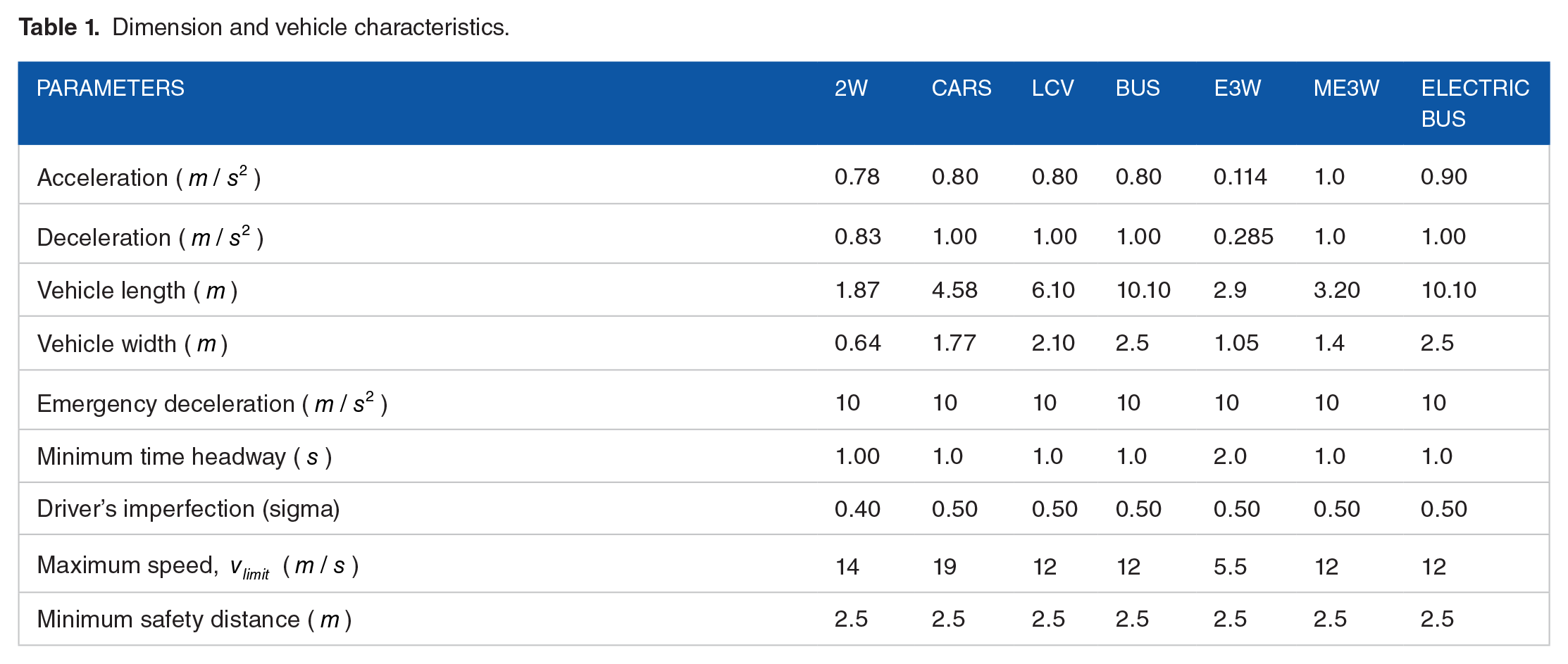
The dimension E3Ws vehicle, characteristics were used as shown in Figure 4. Values were calculated by conducting a pilot survey and random sampling of E3Ws as there is variation in dimension and power. These vehicles are powered by DC motor (brushless) electric motor having power ranging from 0.75 to 0.85 kW.¹⁹ For vehicles other than E3Ws, values were adapted from Amanand Parti.³⁴

Figure 4.

Illustration of electric three wheeler and its attributes.

Model Calibration and Validation

Krauss Model needs to be calibrated to ensure that they represent field-observed traffic conditions closely. For calibration, trial and error methods were adopted since the objective function does not have a closed form. Using an optimization method for such a scenario is difficult.³⁵ The values of acceleration for vehicles other than E3Ws have been adopted from Mahapatra and Maurya.³⁶ For speed, normal distribution has been adopted for vehicles. The parameters varied are Tau (headway), driver imperfection Sigma, lateral resolution value, lane change parameter speedGain and the normal distribution factors namely speedDev and speedFactor. The simulated volumes and real volumes for the main freeway are used to calculate GEH statistics.^37,38

G E H = \sqrt{\frac{{(M_{o b s (n)} - M_{s i m (n)})}^{2}}{(M_{o b s (n)} + M_{s i m (n)}) / 2}}

(5)

$M_{o b s (n)}$ represents the field volumes and $M_{s i m (n)}$ represents the simulated volumes obtained from the simulation in Equation (5). According to the UK Highways Agency’s Design Manual for Roads and Bridges (DMRB), 85% of volumes in the simulated model should have GEH less than 5 for an accurate representation of real-field traffic flow.³⁹ A total of 87% of GEH values have errors less than 5% for the simulated traffic. Table 2 shows the descriptive statistics for GEH values.

Table 2.

Descriptive statistics for GEH.

Detector	Mean	Standard deviation	Maximum value
1	3.05	1.93	5.78
2	3.01	1.87	8.1
3	3.18	1.53	9.05
4	2.17	0.85	6.5

Emission Model

Most exhaust emissions in metropolitan areas come from traditional internal combustion engines.^40,41 Several factors affect the exhaust emissions from vehicles which complicates the task of estimating emissions. The size of the scale used to measure the emissions from vehicles⁴² is one such factor. When it comes to modelling, the amount of exhaust emissions produced is dependent, among other factors, not only on the type of vehicle but also on the number of vehicles that a specific class of car experiences.⁴³ The elements that influence these emissions include, but are not limited to, the type of fuel (petrol or diesel) used, the sophistication of the emission control system, and the vehicle’s operation along with environmental settings.⁴⁴ It has been observed that E3Ws ply on the major roads of cities and slow down traffic in them.⁴⁵ Their slow speed restricts the movement of other fast-moving vehicles.⁴⁶ Moreover, due to the low speed, frequent gear shifts are required, which increase the consumption of fuel and result in increased pollution. To reliably predict emissions from vehicular traffic, emission models are employed. Inputs can come in the form of precise information on the vehicle, such as its engine specifications, the conditions of the drive and the qualities of the fuel.⁴⁷ Simulations of traffic can be a useful supplement to emission models in some cases.⁴⁸ A virtual depiction of real-world traffic scenarios can be created using traffic simulation software. This makes it possible to study the interactions between vehicles as well as the effects those interactions have on the surrounding environment and the well-being of people who use roadways.⁴⁹ Simulators can generate a specific set of vehicle traffic data, allowing valuable information to be provided on the amount of vehicle emissions in comparison to, for instance, air quality. This information may then be used to advise decision-makers in the process of reducing air pollution.⁵⁰

The models that are used to predict the emissions from vehicles are becoming increasingly complex and comprehensive.⁵¹ There is no question that this is linked to the ever-increasing number of vehicles as well as the wide variety of emissions, modifications and fuel types that are being used.⁵² Differentiating between cold start, hot running and other engine thermal states is equally crucial for emission models. In the 1980s and 1990s, researchers worked to build emission models that could estimate emissions from a vehicle’s warmed-up engine for a select few significant emission components using verified test data.⁵³ Modern emission models are based on data from actual road tests conducted under varying driving situations, predict fuel consumption and allow for the estimation of all known exhaust components, both regulated and unregulated.⁵⁴ Early emission models relied on data from only a few dozen automobiles, whereas modern models incorporate information from thousands.⁵⁵ The approach has evolved over the years to include other factors in addition to the traditional modelling for driving mode (acceleration, deceleration, idle and cruise). These variables include information from car engines regarding engine load, speed, temperature, air-to-fuel ratio and other parameters.⁵⁶

HBEFA4 (Handbook Emission Factors for Road Transport) is the latest version of the emission model used for estimating vehicular emissions. It provides factors for pollutants like ${CO}_{2}, CO, {NO}_{x}, PM$ and $VOCs$ based on vehicle characteristics like fuel, speed and vehicle class. HBEFA4 is currently used by SUMO as an emission model. There are various emission models available for estimating emissions in traffic simulation models. They are mainly classified as being macroscopic, mesoscopic and microscopic. The emission models which can be used with the microsimulation model are HBEFA and PHEM. HBEFA is chosen for this study as PHEM does not estimate some important emissions like ${CO}_{2}, {NO}_{2}, {SO}_{2}$ and $N_{2} O$ which can be estimated using HBEFA.⁴³ Also, the PHEM model cannot be used to estimate the emissions from 2-wheelers. The high percentage of 2-wheelers in the present study presents the need to use the HBEFA model along with the microsimulation model. As per the findings of Mądziel⁴³ it is possible to use a macroscopic emission model like HBEFA along with a microscopic traffic model like the Krauss Model. Each vehicle is modelled individually but traffic data is aggregated over a certain fixed duration of time in SUMO. Generating and plotting data for each vehicle for every time step will generate huge data which can time taking to process. The data collected from detectors and cameras are also in aggregated form and it is convenient when calibrating and validation of the model is done. The power demand of vehicle in HBFA is calculated using:

P = c_{0} + c_{1} v a + c_{2} v a^{2} + c_{3} v + c_{4} v^{2} + c_{5} v^{3}

(6)

Where co-efficient of $c_{n}$ are dependent on vehicle type and engine type of vehicle. Emission factors are selected from HBEFA4 data for power demand calculation.

Results and Analysis

For the sake of simplicity Scenario 0, Scenario 1, Scenario 2, Scenario 3 Scenario 4 and Scenario 5 will be referred to as S0, S1, S2, S4, S4 and S5 respectively. After running the simulations it is found that the mean traffic flow falls as the percentage of E3Ws increases on the road. The maximum flow is observed in S0, followed by S5. The minimum value of average traffic flow is observed in S3 (with maximum E3Ws) with a reduction of 49.8%. A similar trend is observed with mean harmonic speed, with a reduction of 28.8% when compared to S0. Mean Harmonic speed is increased by 2.6% for S4 while reduction of HC is maximum for S5 scenario. Figure 5a and b show, respectively, the time series plot of average flow and harmonic mean speed as the percentage of E3Ws increases. For S4 and S5, the median speed is higher than in scenarios with E3Ws.

Figure 5.

(a) Time series plot for traffic flow and (b) time series plot for harmonic mean speed.

The box plot in Figure 6 shows the median speed as 21.67 km/h for S3 and 33.46 km/h for S4. It can also be observed that the distribution of speed data points is spread for scenarios where E3Ws are not present. It is worth mentioning that the maximum percentage of E3Ws is taken as 29.7%, but the speed data points concentrate towards the lower value. For analysing the emissions over the section, a heatmap is plotted, where the x-axis represents the space and the y-axis represents the average emission milligrams per second. The emissions near the on-ramp are high in all scenarios but start decreasing after it. It is observed that emissions decrease with increasing E3Ws. A similar trend is observed with other parameters, as shown in Table 3. These results indicate that the emissions were reduced due to the introduction of slow-moving E3Ws, but this observation needed further analysis. Figure 7 shows the heatmap of emissions for cars along the section of the road under consideration. The spatial distribution of emissions shows an initial high density at the beginning of the road due to the presence of 2 lanes and gradual decreases as the lanes increase to 4. In S1, S2 and S3, it can be observed that the intensity of emissions decreased when compared to S0, but the emissions are more spread due to the reduced speed of cars. For S4 and S5, the intensity is low, but the spread is similar to S1, S2 and S3.

Figure 6.

Box plot for speed for all scenarios.

Table 3.

Emission for all scenarios.

Parameters	Scenario 0	Scenario 1	Scenario 2	Scenario 3	Scenario 4	Scenario 5
$C O_{2}$ (mg/s)	2177.58	1729.72 (−20.6%)	640.53 (−70.6%)	578.01 (−73.5%)	995.80 (−54.3%)	910.83 (−58.2%)
$C O$ (mg/s)	3.092	2.392 (−22.6%)	0.814 (−73.7%)	0.657 (−78.8%)	1.016 (−67.1%)	1.211 (−60.5%)
$H C$ (mg/s)	0.110	0.0789 (−28.3%)	0.0359 (−67.4%)	0.0294 (−73.3%)	0.0433 (−60.6%)	0.0216 (−80.4%)
$N O_{x}$ (mg/s)	2.835	2.222 (−21.6%)	0.9685 (−65.8%)	0.9335 (−67.1%)	1.3310 (−53.1%)	0.8003 (−71.8%)
$P M_{x}$ (mg/s)	0.1607	0.1235 (−23.1%)	0.0424 (−73.6%)	0.0300 (−81.3%)	0.0719 (−55.3%)	0.0592 (−63.2%)
$F u e l$ (mg/s)	697	553.3 (−20.6%)	204.4 (−70.6%)	183.9 (−73.6%)	318.2 (−53.9%)	291.7 (−58.1%)
Average flow (veh/h)	1566	1130 (−27.8%)	810 (−48.2%)	786 (−49.8%)	1426 (−8.9%)	1513 (−3.4%)
Mean harmonic speed (km/h)	32.09	28.08 (−12.5%)	25.49 (−20.6%)	22.86 (−28.8%)	32.91 (+2.6%)	30.57 (−4.7%)

Figure 7.

Heatmap of ${CO}_{2}$ for cars over the section.

Figure 8 shows the spatial spread of ${PM}_{x}$ for all scenarios. For scenario 1, it can be observed that there is a shift in the pattern of emissions, showing an increased frequency of higher emissions. S2 and S3 show distinct separations between high- and low-emission brackets for cars. This can be explained by the higher percentage of slow-moving E3Ws in the traffic stream. These vehicles tend to limit the manoeuvrability of other vehicles, leading to forced lane changes and increased emissions. For S4, ${PM}_{x}$ is similar to all other scenarios with high flow and harmonic speed values. Thus, ME3Ws are best suited for urban traffic, as it can be observed in S1, S2 and S3 that ${PM}_{x}$ emissions are reduced on a macro level due to electric vehicles, but there is an increase in emissions by fuel-driven vehicles.

Figure 8.

Heatmap of ${PM}_{x}$ for cars over the section.

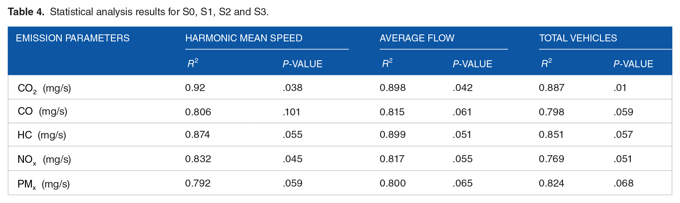
A regression analysis was performed to determine whether the emission reduction is correlated with a decrease in traffic flow caused by an increase in slow-moving E3Ws in traffic. The flow of fuel-driven vehicles is kept constant, and the flow of slow-moving E3Ws is increased progressively from 0% to 29.7% (S0-S3). Table 4 shows the square of the Pearson Correlation Coefficient $(R^{2})$ and the P-value. The value of alpha is taken as .05 for the statistical analysis. It can be seen that for almost all emission parameters, the value of $R^{2}$ is significantly high enough to reject the null hypothesis, indicating a linear relationship between the reduction of the number of vehicles and emission parameters. Similar results are observed for average traffic flow and harmonic mean speed. Figure 9 shows the linear regression line for average ${CO}_{2}$ and the number of vehicles. Thus, it can be inferred from the above analysis that the environmental benefits of E3Ws are not only because of their zero-emission property but also due to the reduced flow of fuel-driven vehicles. In other words, the efficiency of the road is decreased, giving the impression that the presence of slow-moving E3Ws leads to a drastic reduction in emissions.

Table 4.

Statistical analysis results for S0, S1, S2 and S3.

Emission Parameters	Harmonic Mean Speed		Average Flow		Total Vehicles
	$R^{2}$	p-value	$R^{2}$	p-value	$R^{2}$	p-value
$C O_{2}$ (mg/s)	0.92	.038	0.898	.042	0.887	.01
$C O$ (mg/s)	0.806	.101	0.815	.061	0.798	.059
$H C$ (mg/s)	0.874	.055	0.899	.051	0.851	.057
$N O_{x}$ (mg/s)	0.832	.045	0.817	.055	0.769	.051
$P M_{x}$ (mg/s)	0.792	.059	0.800	.065	0.824	.068

Figure 9.

Correlation between number of vehicles and average $C O_{2}$ emission with increasing E3Ws.

Conclusions

In this paper, we present a study investigating the environmental impact of slow-moving E3Ws widely used in India for last-mile connectivity. A total of 6 scenarios were tested using a calibrated microsimulation model with field data. Scenario 1 represented real field conditions, while the rest of the scenarios were developed with different combinations of E3Ws, ME3Ws and electric buses. This allowed the authors to compare the existing and potential traffic conditions in the test section. The authors examined the scenario with the lowest emission and with the lowest traffic flow as well as harmonic mean speed. The presence of slow-moving E3Ws on the test section of an urban road adversely impacted traffic performance parameters like average flow and harmonic mean speed. The average and emission are reduced with an increasing percentage of slow-moving E3Ws. It is also worth mentioning that the rate of addition of fuel-driven vehicles is kept constant in every scenario. A regression analysis shows that the decrease in emissions is attributed to a decreased number of fuel-driven vehicles on the road section. In the hypothetical S4 scenario where slow-moving E3Ws are replaced by enhanced version ME3Ws, which have acceleration, deceleration, and maximum speed comparable to fuel-driven vehicles, the reduction of emissions is up to 67.1% without compromising the traffic performance parameters, average traffic flow, or harmonic mean speed, which showed a decrease of 8.9% and an increase of 2.6%, respectively, over scenario 0. For hypothetical scenario 5, where all 3-wheelers are replaced by electric buses in the relevant proportion, this results in a 3.4% reduction of average traffic flow and a 4.7% reduction of harmonic mean speed. Maximum reduction in HC and ${NO}_{x}$ was observed in this scenario (80.4% and 71.8% respectively) when compared to scenario 0. Thus, it can be concluded that for this study section E3Ws in their current form offset the environmental benefits due to their speed and acceleration characteristics, which are attributed to their lower power capacity. As part of efforts to reduce global warming, these vehicles are looked upon for reducing emissions and often receive subsidies. Therefore, it is necessary to analyse the holistic picture in decision-making by considering a wider network for analysis. The study has been conducted on a limited section and with a short duration therefore in future work more locations shall be considered. This study has not considered the amount of energy emitted during the production of batteries or their recycling costs. The safety aspects that arise due to the speed difference and instability of these vehicles have not been considered. The above issues will be the subject of future research.

Footnotes

Acknowledgements

The authors would like to thank the Integral University Lucknow, India for providing manuscript number: IU/R&D/2024-MCN0002465 for the present research. The authors would like to thank Lucknow Police for the permission to collect traffic data on the road section considered for this research.

Declaration of conflicting interests:

The author(s) declared no potential conflicts of interest with respect to the research, authorship, and/or publication of this article.

Funding:

The author(s) received no financial support for the research, authorship, and/or publication of this article.

Author Contributions

Mohd Sadat has collected the data, reviewed the literature, and written the manuscript. Syed Aqeel Ahmad and Mehmet Ali Silgu have supervised the manuscript. Shrish Bajpai and Digvijay Pandey have reviewed and edited the manuscript. The authors do not have any conflicts of interest with other entities or researchers. All authors have read and agreed to publish a version of the manuscript.

References

Chanana

Sharma

Kumar

, et al. Combustion and stubble burning: A major concern for the environment and Human Health. Fire. 2023;6:79.

Bai

, et al. Investigation of yearly indoor/outdoor PM2. 5 levels in the perspectives of health impacts and air pollution control: Case study in Changchun, in the northeast of China. Sustain Cities Soci. 2020;53:101871.

Dey

Mehta

. Automobile pollution control using catalysis. Resour Environ Sustain. 2020;2:100006.

Trivedi

Prasad

Mishra

Kalam

Yadav

Current scenario of CNG vehicular pollution and their possible abatement technologies: an overview. Environ Sci Pollut Res. 2020;27:39977-40000.

Trivedi

Prasad

Choice of precipitant and calcination temperature of precursor for synthesis of NiCo2O4 for control of CO–CH4 emissions from CNG vehicles. J Environ Sci. 2018;65:62-71.

Galiwango

Bainomugisha

Kivunike

Kateete

Jjingo

Air pollution and mobility patterns in two Ugandan cities during COVID-19 mobility restrictions suggest the validity of air quality data as a measure for human mobility. Environ Sci Pollut Res. 2023;30:34856-34871.

Soni

Singh

Aggarwal

SG.

Comparative measurement of CO2, CH4 and CO at two traffic interjunctions having inflated vehicular flow in Delhi. J Environ Sci. 2024;141:314-329.

Omrani

Goriaux

Liu

Martinet

Jean-Soro

Ruban

. Platinum group elements study in automobile catalysts and exhaust gas samples. Environ Pollut. 2020;257:113477.

Tsoi

Loo

Zhang

. The co-benefits of electric mobility in reducing traffic noise and chemical air pollution: Insights from a transit-oriented city. Environ Int. 2023;178:108116.

10.

Requia

Mohamed

Higgins

Arain

Ferguson

How clean are electric vehicles? Evidence-based review of the effects of electric mobility on air pollutants, greenhouse gas emissions and human health. Atmos Environ. 2018;185:64-77.

11.

Bansal

Gadepalli

AitBihiOuali

Eliciting mobility preferences of Indians for E-rickshaws: evidence from Gurugram. Transp Policy. 2023;134:19-30.

12.

Coban

Rehman

Mohamed

Analyzing the societal cost of electric roads compared to batteries and oil for all forms of road transport. Energies. 2022;15:1925.

13.

Ray

Rana

Mishra

Davies

Sepasi

. Battery-swap technology for e-rickshaws: challenges, opportunity and scope. In: 2020 21st national power systems conference (NPSC), December, IEEE;2020:1-6.

14.

Sanguesa

Torres-Sanz

Garrido

Martinez

Marquez-Barja

JM.

A review on electric vehicles: technologies and challenges. J Smart Cities. 2021;4:372-404.

15.

Sun

Wang

Technology development of electric vehicles: a review. Energies. 2019;13:90.

16.

Sharma

View: transport sector emissions and moving ahead. The Economic Times, 2021.

17.

Wasim

Abadel

Bakar

Alshaikh

. Future directions for the application of zero carbon concrete in civil engineering-A review. Case Stud Constr Mater. 2022;17:e01318.

18.

Anika

Nnabuife

Bello

Okoroafor

Kuang

Villa

. Prospects of low and zero-carbon renewable fuels in 1.5-degree net zero emission actualisation by 2050: A critical review. Carbon Capture Sci Technol. 2020;5:100072.

19.

Majumdar

Jash

Merits and challenges of e-rickshaw as an alternative form of public road transport system: a case study in the state of West Bengal in India. Energy Proc. 2015;79:307-314.

20.

Singh

Mishra

Tripathi

. Analysing acceptability of E-rickshaw as a public transport innovation in Delhi: A responsible innovation perspective. Technol Forecast Soc Change. 2021;170:120908.

21.

Nadimuthu

LPR

Victor

Performance analysis and optimization of solar-powered E-rickshaw for environmental sustainability in rural transportation. Environ Sci Pollut Res. 2021;28:34278-34289.

22.

Munigety

Vicraman

Mathew

. Semiautomated tool for extraction of microlevel traffic data from videographic survey. Transp Res Rec. 2014;2443(1):88-95.

23.

Lertworawanich

Unhasut

A CO emission-based adaptive signal control for isolated intersections. J Air Waste Manag Assoc. 2021;71:564-585.

24.

Chandra

Mehar

Velmurugan

Effect of traffic composition on capacity of multilane highways. KSCE J Civil Eng. 2016;20:2033-2040.

25.

Mondal

Saha

Passing behaviour on two-lane suburban arterials: an observation under mixed traffic with a significant fraction of battery-run e-rickshaws. Innov Infrastruct Solut. 2020;5:22.

26.

Panta

Gairola

Nezamuddin

Modelling benefit-to-cost ratio for initial phase electrification using battery electric bus. Transp Policy. 2024;145:137-149.

27.

Yadav

Singh

Anand

, et al. Ecological model analysis of respiratory health risk factors by ambient air pollution in Lucknow, the capital city of Uttar Pradesh, India. GeoJournal. 2022;87:469-483.

28.

Kumar

Mishra

Chandra

Hussain

Evaluation of urban transport-environment sustainable indicators during odd–even scheme in India. Environ Dev Sustain. 2021;23:17240-17262.

29.

Abuamer

Sadat

Tampère

. A comparative evaluation of ramp metering controllers ALINEA and PI-ALINEA. In: 2018 International conference on computational and characterization techniques in engineering & sciences (CCTES), September, IEEE;2018:127-131.

30.

Munigety

Mathew

TV.

Towards behavioral modeling of drivers in mixed traffic conditions. Transp Dev Econ. 2016;2:20.

31.

Treiber

Kesting

. Traffic Flow Dynamics. Traffic Flow Dynamics: Data, Models and Simulation. Springer-Verlag; 2013:983-1010.

32.

Lopez

Behrisch

Bieker-Walz

, et al. Microscopic traffic simulation using sumo. In: 2018 21st international conference on intelligent transportation systems (ITSC), November, IEEE;2018:2575-2582.

33.

Chandra

Gangopadhyay

Velmurugan

Ravinder

. 2017). Indian highway capacity manual (Indo-HCM).

34.

Aman

Parti

Estimation of passenger car unit for undivided Two-Lane roads in the mountainous region. J Inst Eng (India) Ser A. 2021;102:185-197.

35.

Asaithambi

Kanagaraj

Srinivasan

Sivanandan

Study of traffic flow characteristics using different vehicle-following models under mixed traffic conditions. Transp Lett. 2018;10:92-103.

36.

Mahapatra

Maurya

AK.

Dynamic parameters of vehicles under heterogeneous traffic stream with non-lane discipline: an experimental study. J Traffic Transp Eng. 2018;5:386-405.

37.

Sadat

Celikoglu

HB.

Simulation-based variable speed limit systems modelling: an overview and a case study on Istanbul freeways. Transp Res Procedia. 2017;22:607-614.

38.

Sadat

Abuamer

Ali Silgu

Berk Celikoglu

Comparative performance analysis of variable speed limit systems control methods using microsimulation: a case study on D100 Freeway, Istanbul. In: Computer Aided Systems Theory–EUROCAST 2017: 16th International Conference, Las Palmas de Gran Canaria, Spain, February 19-24, 2017, Revised Selected Papers, Part II 16. Springer International Publishing; 2018:462-449.

39.

UK Highways. Agency’s Design Manual for Roads & Bridges (DMRB), 2011.

40.

Wallington

Anderson

Dolan

Winkler

SL.

Vehicle emissions and urban air quality: 60 years of progress. Atmosphere. 2022;13:650.

41.

Piracha

Chaudhary

MT.

Urban air pollution, urban heat island and human health: a review of the literature. Sustainability. 2022;14:9234.

42.

Franco

Kousoulidou

Muntean

, et al. Road vehicle emission factors development: a review. Atmos Environ. 2013;70:84-97.

43.

Mądziel

Vehicle emission models and traffic simulators: a review. Energies. 2023;16:3941.

44.

Dutta

Chavalparit

. Assessment of health burden due to the emissions of fine particulate matter from motor vehicles: A case of Nakhon Ratchasima province, Thailand. Sci Total Environ. 2023;872:162128.

45.

Das

. Problem and Prospect of E-Rickshaw–An Overview. CONSCIENTIA Academic Journal of Krishnagar Government College. 2018;6:47-58.

46.

Kumar

Mondal

Saha

Roy

SK.

, September). Characteristics of e-rickshaw dominated mixed-mode traffic in suburban arterial corridors. In: International conference on transportation infrastructure projects: conception to execution, September, Springer Nature;2022:261-276.

47.

Yildiz

Caliskan

Mori

. Effects of cordierite particulate filters on diesel engine exhaust emissions in terms of pollution prevention approaches for better environmental management. J Environ Manage. 2021;293:112873.

48.

Samaras

Tsokolis

Toffolo

, et al. Enhancing average speed emission models to account for congestion impacts in traffic network link-based simulations. Transp Res D Transp Environ. 2019;75:197-210.

49.

Chao

, et al. A survey on visual traffic simulation: models, evaluations, and applications in autonomous driving. Comput Graph Forum. 2020;39:287-308.

50.

Oulha

Pace

Ouafi

Luca

. Traffic control strategies based on internet of vehicles architectures for smart traffic management: centralised vs. decentralised approach. Int J Comput Eng Sci. 2023;26:528-536.

51.

Agarwal

Mustafi

. Real-world automotive emissions: Monitoring methodologies, and control measures. Renew Sust Energ Rev. 21;137:110624.

52.

Wang

Gong

Estimation of bus emission models for different fuel types of buses under real conditions. Sci Total Environ. 2018;640-641:965-972.

53.

Joshi

Review of vehicle engine efficiency and emissions. SAE Int J Adv Curr Pr Mobil. 2020;2:2479-2507.

54.

Ahire

Shewale

Razban

A review of the state-of-the-art emission control strategies in modern diesel engines. Arch Comput Methods Eng. 2021;28:4897-4915.

55.

Pinto

Kumar

Alonso

, et al. Traffic data in air quality modeling: a review of key variables, improvements in results, open problems and challenges in current research. Atmos Pollut Res. 2020;11:454-468.

56.

Bui

KHN

. An automated hyperparameter search-based deep learning model for highway traffic prediction. IEEE Trans Intell Transp Syst. 2021;22:5486-5495.

A Study on Environmental Impact of Slow Moving Electric Vehicles Using Microsimulation on Lucknow Urban Road With an On-Ramp

Abstract

Background:

Methods:

Results:

Conclusion:

Keywords

Introduction

Background

Methodology

Study Area

Mixed Traffic Modelling

Model Calibration and Validation

Emission Model

Results and Analysis

Conclusions

Footnotes

Acknowledgements

Declaration of conflicting interests:

Funding:

Author Contributions

References