Modeling the Propagation of Landslide-Derived Flow in Tropical Mountain Basins: La Liboriana and La Argelia Basins (Colombia)

Abstract

Debris flows are destructive movements of water and earth, strongly influenced by environmental factors. In South America, extensive tropical forests, mountain chains, and high annual rainfall create favorable conditions for these geodynamic processes. However, there is still a need for further research on the triggers, soil mechanics, climate influence, and travel distances of such events. This study explores three physically based models for simulating the propagation of shallow landslides and associated flows in data-scarce regions, with the aim of developing a comprehensive analysis methodology for these events, the affected zones, and the processes that cause them. Using the 2015 Salgar landslide in Antioquia, Colombia, as a calibration case, where over 40 landslides triggered by a storm resulted in significant loss of life and property damage, three models were calibrated and evaluated: RAMMS, Flow R, and GPP from SAGA GIS. Following this, the models were validated using a similar event in the La Argelia basin, Carmen de Atrato, Chocó. Statistical analyses and ROC curve evaluations were conducted to assess the predictive performance of these models, considering the available data and event documentation. The findings suggest that while the models are useful for hazard assessments in tropical mountain basins, further refinement and data collection are essential to improve predictive accuracy. This research contributes to understanding landslide dynamics in tropical regions and offers insights for future hazard mitigation efforts.

Introduction

Landslides represent a significant global threat, with economic and human consequences that surpass those of many other natural hazards. Over the past 40 years, natural disasters have caused over 3.3 million deaths and 2.3 trillion dollars in economic losses worldwide, with landslides accounting for approximately 17% of disaster-related fatalities (Vega et al., 2019, 2023). Although developed countries like the United States and Japan report relatively few deaths, the economic impact is considerable, with annual losses ranging between 1 and 6 billion dollars (Vega et al., 2019, 2023). In Colombia, natural disasters between 1970 and 2011 resulted in losses amounting to 7.1 billion dollars, with landslides responsible for 5% of this total and average annual losses of 177 million dollars (Vega et al., 2019, 2023). In regions such as the Aburrá Valley, landslides are particularly devastating, contributing to 35% of building damages and 74% of disaster-related deaths (Vega et al., 2019).

The importance of landslide risk is particularly pronounced in tropical and mountainous countries within the Circum-Pacific region, where rainfall-induced landslides are among the most frequent causes of natural disasters. This complex issue must be addressed due to its severe economic impacts and the associated loss of life, including costs related to relocating communities, rebuilding infrastructure, and restoring water quality in affected water sources (Vega & Hidalgo, 2016). In countries like Colombia, the landslide events that result in the greatest number of fatalities and economic losses are often linked to sudden river or stream floods generated by landslides in the watersheds (Hidalgo & Vega, 2021). Debris flows in South America, influenced by the Andean geography and climate, exhibit unique characteristics: intense rainfall and phenomena such as La Niña often trigger avalanches that rapidly evolve into torrential flows that impact populated areas, as documented in recent disasters in Colombia (Tarazá 2007, Salgar 2015, Mocoa 2017, Dabeiba 2020), Brazil (Serra do Mar), Chile (Ñisoleufu, Chaiguaco), and Argentina (Aconcagua; Moreiras et al., 2021; Vergara et al., 2019).

The response of South American mountains to these events depends on various triggering mechanisms, including intense rainfall, snowmelt, and earthquakes, in combination with high social vulnerability (Arango & Aristizábal, 2023; Palacio et al., 2025). In the semi-arid Central Andes, climate change and seasonal snowmelt are key drivers (Moreiras et al., 2021; Vergara et al., 2019), whereas in the southern Andes, glaciovolcanic landscapes and intense rainfall dominate as controlling factors (Fustos et al., 2025; Maragaño-Carmona et al., 2025). Determining landslide-prone areas is therefore crucial for preserving lives and reducing economic losses, particularly in developing countries located in tropical mountainous regions repeatedly affected by extreme rainfall and tectonic activity (Frodella et al., 2022; Pradhan & Kim, 2016). Global patterns of landslide-induced fatalities consistently highlight Andean regions as hotspots, due to the combination of steep relief, active tectonics, and high-intensity precipitation (Frodella et al., 2022; Petley, 2012).

The physical processes involved in the occurrence of debris flows triggered by landslides within a basin are complex, and the relationships along the rainfall–landslide–debris flow chain in a changing geodynamic environment remain only partially resolved (C. Li et al., 2023). Modeling these phenomena typically addresses each stage separately; however, there is a recognized need to develop approaches that better integrate the different components of this chain (Vega et al., 2024). Previous studies have evaluated rainfall-triggered landslides (Hong et al., 2020; Quan Luna et al., 2014), landslides induced by the combined effects of rainfall and earthquakes (Cheng et al., 2018), and coseismic landslides (C. Li et al., 2023). Initial slope failure is usually assessed using limit equilibrium or stress–deformation methods, requiring coupled modeling of rainfall, infiltration, and their effects on soil strength (Hidalgo et al., 2017; C. Li et al., 2023). Assessing landslide runout is critical for hazard estimation, and two main approaches are commonly used: empirical or statistical methods based on observed correlations, and analytical or numerical methods grounded in physical processes (Abraham et al., 2025; Giarola et al., 2024; Hungr et al., 2005; McDougall, 2017).

Empirical and statistical methods have evolved from simple relationships between mobilized volume, travel distance, and deposition angle (Hungr et al., 2005; McDougall, 2017) toward models that capture more complex dependencies across different triggers (rainfall, earthquakes, or their combination) and material types (rockslides, landslides, and mixed-material slides; Gong et al., 2025). In parallel, machine learning methods such as neural networks and other algorithms are increasingly used to model debris flow susceptibility and mobility (Bhuyan et al., 2025; Crescenzo et al., 2024; Giarola et al., 2024; Santi et al., 2025). Analytical and numerical models, rooted in hydrodynamic theory and adapted for non-Newtonian rheologies, drag, and other complexities, can simulate variables such as flow height and velocity in space and time (Abraham et al., 2025). While some recent developments couple the entire failure and runout process (X. Li et al., 2025), most applications remain focused on runout assessment (Abraham et al., 2025; Pudasaini & Mergili, 2019; Sun et al., 2024; Takebayashi & Fujita, 2020; Wichmann, 2017). Technological advances have enabled the development of several computational tools to estimate runout length and inundation areas, including RAMMS, Flow-R, and the Gravitational Process Path (GPP) model implemented in SAGA GIS (McDougall, 2017; Wichmann, 2017).

RAMMS, developed by the WSL Institute for Snow and Avalanche Research SLF, has been widely applied to reproduce well-documented debris flow and avalanche events in alpine environments, where detailed records of volumes and rheological parameters are often available (Cesca & D’Agostino, 2008; Frank et al., 2015; Hussin et al., 2012). Applications include events in the Swiss and Italian Alps, and in Serbia under extreme rainfall conditions over highly weathered materials (Krušić et al., 2019). Flow-R is an application designed primarily for regional-scale debris flow assessment, supporting the identification of potential source areas and runout extent, and has been used mainly in alpine and high-mountain environments for back-analysis and susceptibility mapping (Pastorello et al., 2017; Xu et al., 2022; Ye et al., 2023). The GPP module of SAGA GIS is a GIS-based framework that simulates process paths and runout areas from digital terrain models using flow-direction and process-path algorithms, and has been applied to analyze sediment cascades, process connectivity, and sediment transfer in mountain catchments (Kofler et al., 2022; Goetz et al., 2021; Wichmann, 2017).

Despite these developments, the performance and transferability of such models in tropical mountain regions with scarce data remain insufficiently explored. Many global and regional landslide and disaster databases still underrepresent South American mountain environments, and several studies highlight how data scarcity, dense vegetation, complex terrain, and limited accessibility hinder robust landslide modeling exactly where risk is highest (e.g. Colombian Andes). In Colombia, recent work using the open-source, physically based r.slope.stability model in the La Arenosa catchment has demonstrated that probabilistic GIS-based analyses can achieve reasonable performance under intense tropical rainfall and deep weathering profiles but also revealed sensitivities to geotechnical parameterization and the value of combining multiple physically based approaches (Palacio Cordoba et al., 2020). Studies in Perú highlight the need to consider Newtonian and non-Newtonian flows in hydraulic modeling (Chacón et al. 2025). Research in the Serra do Mar of Brazil highlights the role of these flows in local geomorphology (Villaça et al. 2022). Despite the needs outlined above and the high impact of landslides, few studies exist in Soth America that allow us to better understand the dynamics of these phenomena. This evidence shows that regional empirical validation of existing open-source tools is critical to support land-use planning and disaster risk reduction in tropical mountainous settings.

In this context, multi-model comparative studies are particularly relevant. Using different runout tools in parallel helps identify model-specific biases and applicability limits (e.g. sensitivity to digital elevation model resolution, simplified rheologies, or uncertainties in source areas) and can increase the robustness of hazard zonation in basins with limited inventories and monitoring information. For tropical Andean catchments, where rainfall-induced multi-landslide events frequently generate destructive debris flows but detailed event documentation is scarce, comparative validation of existing open-source models can provide practical guidance for selecting and configuring tools for risk assessment. Moreover, such studies build directly on established methodological frameworks like GPP, RAMMS, and Flow-R, emphasizing their empirical evaluation under new geomorphological and climatic conditions rather than proposing entirely new modeling approaches (McDougall, 2017; Wichmann, 2017).

The primary objective of this study is therefore to present a regional, empirical multi-model validation of the RAMMS, Flow-R, and GPP models for debris flow propagation in data-scarce Andean tropical basins. The La Liboriana basin in Salgar, Antioquia, affected by a devastating debris flow in May 2015 triggered by multiple rainfall-induced landslides, is used as a calibration case, constrained by available geomorphological, hydrometeorological, and impact information (Hidalgo & Vega, 2021; Hoyos et al., 2019; Marín et al., 2021; Ruiz-Vásquez & Aristizábal, 2018; Vega & Hidalgo, 2021; Velásquez et al., 2020). Model transferability is then evaluated in the La Argelia basin in Carmen de Atrato, Chocó, which exhibits similar topographic and climatic characteristics but lacks a detailed debris-flow monitoring record. Through this design, the study (i) provides a multi-model empirical validation of debris flow propagation tools under pronounced data scarcity typical of Andean tropical basins; (ii) delineates the applicability limits of each model given the use of moderate-resolution DEMs and limited landslide inventories; and (iii) offers a comparative perspective that explicitly acknowledges and builds upon the foundational theoretical contributions of GPP and other existing state-of-the-art models, orienting the contribution toward regional model validation for disaster risk assessment rather than methodological innovation (McDougall, 2017; Palacio Cordoba et al., 2020; Wichmann, 2017).

Materials and Methods

This study analyzes associated debris flows (movement of earth material resembling a fluid), according to the landslide classification by Varnes as detailed by Hungr et al. (2001). The proposed methodology for assessing the travel distance of landslides in the La Liboriana basin follows a multi-model approach, outlined as follows. The first step involves estimating the depth of the soil susceptible to sliding. Second, modeling was conducted using Flow-R. The third step simulates the propagation of debris flow using the RAMMS model (Bartelt et al., 2017). The fourth step included employing the GPP model. Finally, results were compared using performance evaluation techniques. Detailed descriptions of each methodological step are provided in the following sections. All models were applied in the La Liboriana and La Argelia basins.

Study Cases: Calibration and Validation

For the development of this work, two cases were selected for the calibration of the models and the validation of the results obtained during the calibration. To calibrate the selected models, a well-documented case study was chosen, allowing for rigorous validation and ensuring robust results. The availability of precise and detailed data in this case of study facilitates the evaluation of model performance and its application in similar contexts. As part of this research, it was important to determine whether the model calibration done in the previous case could be applied to any basin with similar topographic, climatic, altimetric, and geological characteristics, or if, on the contrary, the models needed to be calibrated specifically for each basis. Figure 1 presents the location of each case and Figure 2 the inventory of landslides.

Figure 1.

Location of the La Argelia and La Liboriana basins in the northwestern Andes of Colombia.

Figure 2.

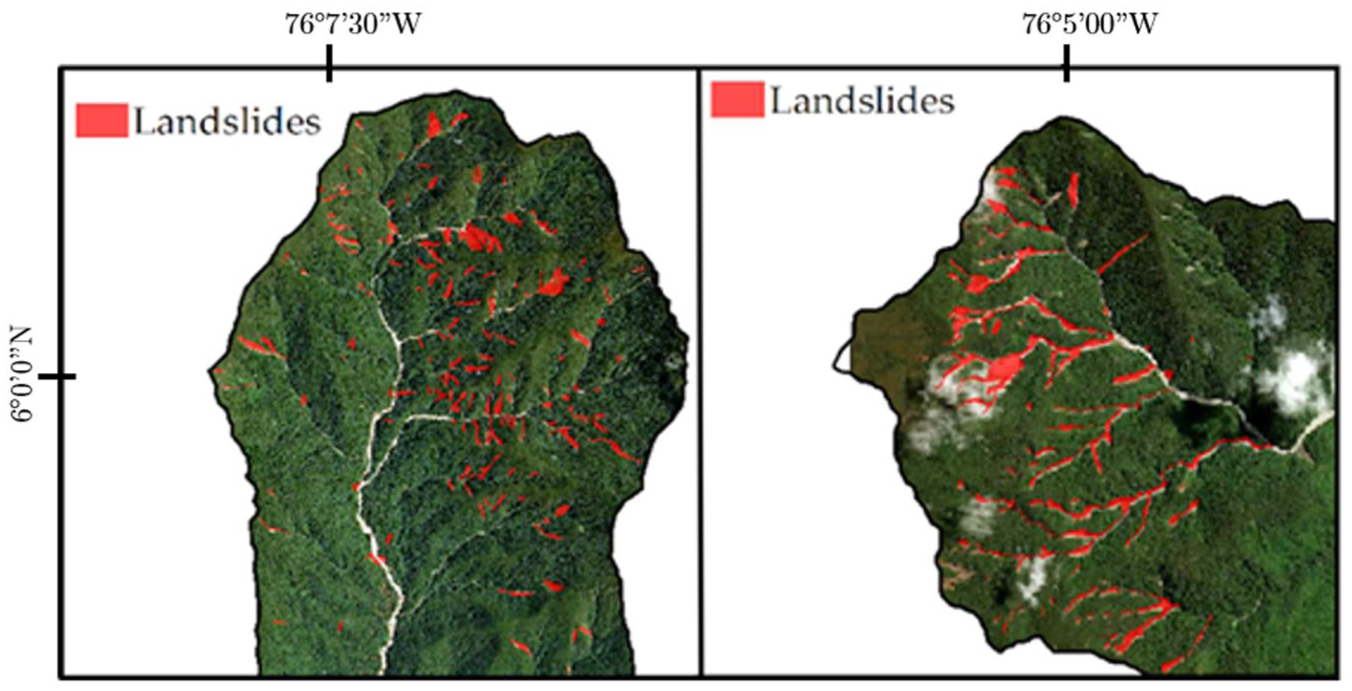
Landslides inventories for the La Argelia (left) and La Liboriana (right) basins. Red polygons indicate mapped landslides derived from high-resolution imagery.

Calibration Case – La Liboriana Basin

To calibrate the selected models, a well-documented case study was chosen, allowing for rigorous validation and ensuring robust results. The availability of precise and detailed data in this case study facilitates the evaluation of model performance and its application in similar contexts.

In 2015, in the municipality of Salgar, Antioquia, Colombia, a series of landslides triggered by heavy rainfall occurred in the La Liboriana basin, which caused the river to be dammed (Velásquez et al., 2020). When the dam broke, it destroyed several homes and claimed over 100 lives. This case was selected for analysis because it is well documented (García-Aristizábal et al., 2019; Hidalgo & Vega, 2021; Hoyos et al., 2019; Velásquez et al., 2020), with an inventory of landslides built from multitemporal satellite image analysis (Ruiz-Vásquez & Aristizábal, 2018), including the timing, magnitude, and duration of the triggering rainfall, as well as the economic and human losses.

Salgar is in the central-western part of Colombia, in the southwestern region of the department of Antioquia. The municipality sits at an altitude of 1,250 m above sea level. The hydrology and climate of this area are characteristic of a mountainous tropical region, featuring a humid, temperate climate, several creeks, and the San Juan River basin. The average annual temperature is 22°C, and annual precipitation is 3,073 mm, with two rainy seasons peaking in May and October.

The municipality is situated in one of the country’s major mountain ranges, the central Andes. The geological environment of the La Liboriana basin is dominated by sedimentary rock formations from the Cretaceous period (shales, siltstones, sandstones, cherts, and conglomerates with some intercalations), along with an intrusive body from the Miocene period. These rock bodies undergo severe in-situ weathering due to the humid tropical climate, forming saprolite and well-developed residual soils (Hidalgo & Vega, 2021).

The geomorphology consists of a rugged mountainous region with narrow valleys and steep slopes covered by forests in the upper areas. In the higher parts, there are fields of crops and deep tropical forests, while in the middle and lower sections of the basin, there are grasslands, coffee plantations, and pasture lands near the stream.

La Liboriana basin is characterized by steep slopes and a humid tropical climate. Cerro Plateado, where the stream originates, is the highest point in the basin, reaching 3,609 m above sea level. Approximately 67% of the total basin area has a slope gradient exceeding 30°. Figure 3 shows the slope map and the variation in the angle of friction of the most superficial soils.

Figure 3.

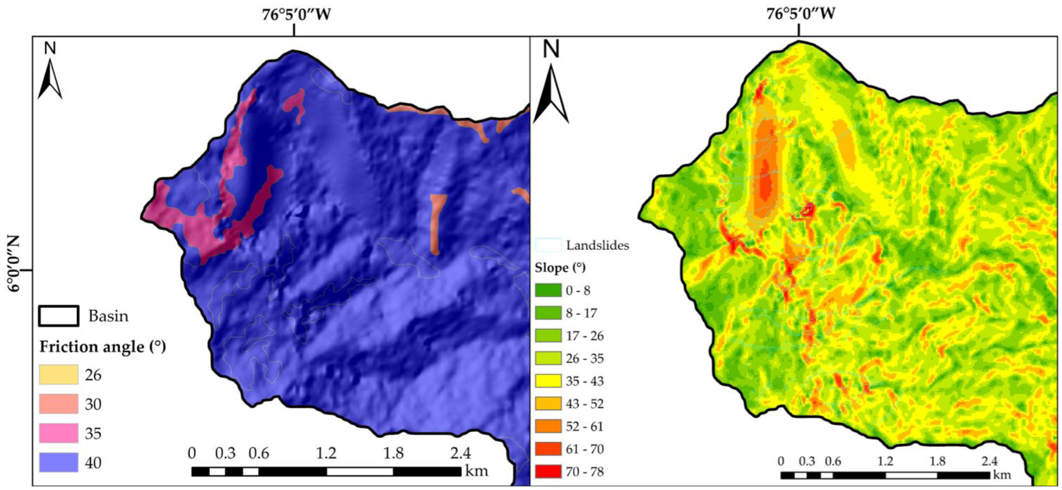
La Liboriana basin: (A) Map of friction angle distribution and (B) Slope map extracted from DEM.

Validation Case – La Argelia Basin

As part of this research, it was important to determine whether the model calibration done in the previous case could be applied to any basin with similar topographic, climatic, altimetric, and geological characteristics, or if, on the contrary, the models needed to be calibrated specifically for each basin.

La Argelia basin, located in the municipality of Carmen de Atrato in the department of Chocó, was chosen for this purpose. This basin has an inventory of landslides that was created from a multitemporal analysis of images obtained using the SAS Planet software, like the method used by Ruiz-Vásquez and Aristizábal, in which both the scars and bodies of each landslide were digitized. This is the only available information that can be compared with the results obtained from this validation.

According to the municipality’s Territorial Organization Scheme (EOT in Spanish), three dominant climates are present in Carmen de Atrato: cold, very humid temperate, and very humid warm, with the cold climate being predominant in the basin. This thermal zone encompasses the upper parts of the western slope of the Western Cordillera between 2,000 and 3,000 m above sea level, which includes the Farallones del Citará. Additionally, according to data from the explanatory notes of the Colombian Geological Service (SGC) geological map sheet 165 for Carmen de Atrato (1986), this area is identified as a very humid montane forest, with a temperature range between 12°C and 18°C, and an average annual rainfall of 2,000 to 4,000 mm.

Carmen de Atrato is a mountainous area with steeply sloping ravines and poorly or moderately developed soils, generally unsaturated, with exposed rock outcrops, and in some places, residues of volcanic ash. The predominant geological formation in the La Argelia basin is the Barroso Formation, which is part of the Cañasgordas Group. This formation contains rocks such as spilites, diabases, basalts, porphyritic basalts, agglomerates, and breccias. To the north of Carmen de Atrato, lenticular diabase bodies with dark chert intercalations can be found. Figure 4 shows the slope map and the variation in the angle of friction of the most superficial soils.

Figure 4.

La Argelia basin: (A) Map of friction angle distribution and (B) Slope map extracted from DEM.

A comparison was made of the most representative characteristics of the two basins to verify that the proposed methodology is applicable to both as shown in Table 1. From the average elevation, temperature, precipitation values, and slope data, it is possible to conclude that the basins are similar, especially in terms of their climatic characteristics, as both belong to a tropical region with intense rainfall cycles.

Table 1.

Comparison between basin characteristics.

CHARACTERISTIC	LA LIBORIANA	LA ARGELIA
Average elevation (msnm)	2,487	2,500
Temperature (°C)	22	18
Average slope (°)	30	30
Annual precipitation (mm)	3,073	2,500
Land use	Agriculture	Forest exploitation
	Pastures	Agriculture
		Cattle

Cartographic Base

All models used require a digital elevation model (DEM) as input. Recent studies have shown that DEM resolution is a variable that influences the accuracy of landslide modeling (Qiu et al. (2022) and that higher DEM resolution allows for more detailed maps that are of great help in urban planning (Karakas et al., 2022). However, it has been shown that 10 or 12.5 m resolution models generate satisfactory results in regional studies (Iqbal et al., 2021; Ortiz et al.,2023; Qiu et al., 2022). Therefore, in this work we use a digital elevation model (DEM) with a cell size of 12.5 m × 12.5 m, obtained from the ALOS PALSAR satellite mission (www.search.asf.alaska.edu). Additionally, a raster containing the seeds, scarps, or initiation points of the landslides was used, identified through multi-temporal analysis of satellite images of the area, along with terrain slope, aspect map, and curvature information. In this context, the input parameters labeled with number 1 correspond to the DEM, seeds, slope, and curvature. The input parameters labeled with number 2 correspond to the DEM, seeds, slope, and aspect.

Rasters containing data on seeds, scarps, and potential landslide initiations identified through multi-temporal analysis of satellite imagery were also employed, along with information on slope, aspect, and curvature of the terrain (FIGEO, 2016).

Sliding Susceptible Soil Depth

Sliding susceptible soil Depth is an essential data point in analyzing problems involving hydrological processes occurring on slopes, as well as the stability of slopes (Montoya-Botero, 2018).

The model used to calculate this depth is based on the behavior of soil in relation to the terrain’s slopes, considering that the flatter a region is, the greater the action of deposition and accumulation of unconsolidated material. Therefore, as the angle of inclination increases, the rate of accumulation decreases (Montoya-Botero, 2018). The model for soil susceptible to sliding is represented by Equation 1. Model for calculation of soil depth susceptible to sliding (Montoya-Botero, 2018).

$$\begin{array}{l}{Z}_s=\left(Z_{s_{\max }}-Z_{s_{\min }}\right)\times \left\{\left[1-\frac{1}{\tan {\theta }_{\lim }}\tan \theta \right]\times \left[\tan h\tan h\left(a\times x\right)\right]\right\}\\ +Z_{s_{\min }}\end{array}$$

(1)

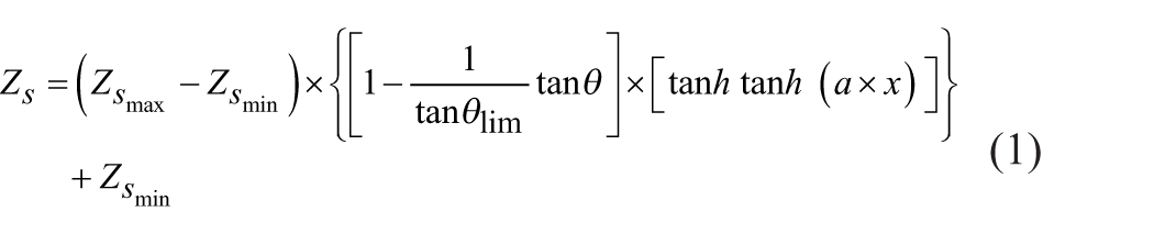
Where Z_s is the resulting soil depth susceptible to sliding [m], Z_smax is the maximum depth of unconsolidated soil anticipated in the study area [m], Z_smin is the minimum depth of unconsolidated soil observed in the study area [m], θ is the slope value on the hillside [°], θ_lim is the slope value established as the influence limit for soil layer alteration (for values greater than this slope, no soil formation occurs) [°], α is a dimensionless parameter that controls the curvature of the terrain, and x is the horizontal distance from a considered point to the nearest drainage [m].

θ_lim refers to the inclination beyond which the effect of this factor no longer interferes with variations in soil depth, meaning that slope values equal to or greater than the established level represent areas where the depth of soil susceptible to sliding is minimal, negligible, or even zero. Figure 5 shows the soil thickness maps of both basins.

Figure 5.

Spatial distribution of soil depth corresponding to the classification proposed by Montoya-Botero (2018): (A) La Liboriana basin and (B) La Argelia basin.

Flow R – Regional Scale Gravitational Hazard Flow Path Modeling

Flow R (Horton et al., 2013) is software that evaluates the regional susceptibility of debris flows through analysis on a GIS platform. A susceptibility map is the primary outcome, enabling the identification of potential source areas and their possible propagation extent. It is important to note that with Flow R, it is possible to obtain results related to the probability of a landslide following a specific flow direction from a cell previously designated as the initiation site of movement.

To evaluate propagation, the software uses two types of algorithms: the flow path algorithm and debris flow propagation, along with friction laws to determine eccentricity.

In the case of the Holmgren algorithm, which is recommended by the developers for analysis, the software calculates the susceptibility proportion in direction i based on the Equation 2 for Holmgren multiple Flow algorithm (Horton et al., 2013).

$$p_i^{fd}=\frac{{(\tan {\beta }_i)}^x}{{{\displaystyle \sum }}_{j=1}^8{(\tan {\beta }_j)}^x}\forall \{\tan \beta >0x\epsilon [1;+\infty [,$$

(2)

Where i, j are the flow directions, $p_i^{fd}$ is the proportion of susceptibility in direction i, $\tan {\beta }_i$ is the slope gradient between the central cell and the cell in direction i and x is the exponent controlling flow divergence.

The model was configured according to the chosen flow direction algorithm, calculation method, and inertia algorithm for each simulation.

The calculation method refers to the type of simulation run. The software offers three options for this: “Overview,” which evaluates only the upper sources of each landslide; “Quick,” which evaluates the upper sources and, at a later analysis stage, propagates the remaining sources, stopping if a previous propagation with higher energy and susceptibility values is encountered; and “Quick,” which activates all origin areas without verifying previous propagations, ensuring that no area is overlooked. The “Quick” method was used in the simulations as it provides detailed information on the total extent of landslides.

The software allows for the evaluation of nine flow direction algorithms based on the D8 algorithm. These algorithms analyze the possible flow directions by comparing the height of neighboring cells. All algorithms were tested, and their results were analyzed in relation to the scar inventory of the basin, as detailed in the model calibration chapter. A total of 20 simulations were performed using this software, based on the characteristics of the input parameters. The combinations are shown in Table 2.

Table 2.

Setup of executed tests in Flow R.

Simulation	1	2	3	4	5	6	7	8	9	10
Input parameters	1	1	1	1	1	1	1	1	1	1
Flow direction algorithm	HM	H	D8	D	Rho8	F	Q	W	G	HM
Simulation	11	12	13	14	15	16	17	18	19	20
Input parameters	1	1	1	1	1	2	2	2	2	2
Flow direction algorithm	HM	HM	HM	HM	HM	HM	HM	HM	HM	HM

*1: DEM, Seeds, Slope, Curvature; 2: DEM, Seed, Slope, Aspect. **H: Holmgren algorithm, HM: Holmgren Modified Algorithm, F: Freeman algorithm, Q: Quinn algorithm, W: Wichmann algorithm, G: Gamma algorithm.

The inertia algorithm is based on a persistence function, as shown in the Equation 3 for the persistence function (Horton et al., 2013).

$$p_i^p={\omega }_{\alpha (i)}$$

(3)

Where $p_i^p$ is the proportion of flow in direction i and $\alpha (i)$ is the angle between the previous direction and the direction from central cell to cell i. This algorithm aims to replicate the behavior of inertia by giving weight to the previous flow direction evaluated (Horton et al., 2013).

The software offers three options for the persistence function: “Proportional,” “Cosines,” and “Gamma (2000)” as shown in Table 3. In all cases, the flow direction that allows for backward movement is assigned to a value of zero (0) to prevent backward propagation. For this case, the Gamma (2000) option was always chosen, as it gives the highest weight to the most likely direction $({\omega }_0)$ for the flow to move.

Table 3.

Persistence function weights (Horton et al., 2011).

	W0	W45	W90	W135	W180
Proportional	1	0.8	0.4	0	0
Cosines	1	0.707	0	0	0
Gamma (2000)	1.5	1	1	1	0

RAMMS – 3D Bidirectional Mass Movement Modeling in Alpine Terrain

RAMMS (Rapid Mass Movements) is a software package that includes three different modules for modeling avalanches, debris flows, and rockfalls (Bartelt et al., 2017). This software is based on the Voellmy fluid model, which is a single-phase approach where shear deformation is completely ignored. Equation 4 shows the formula to calculate included in the Voellmy model (Bartelt et al., 2017).

$$S=\mu \rho Hg\cos \varphi +\left(\frac{\rho g{u}^2}{\xi }\right)$$

(4)

Where $\mu$ is a Coulomb friction coefficient [dimensionless], $\rho$ is the density [kg/m³] g is the acceleration due gravity [m/s²], $\varphi$ is the slope angle [°], h is the flow height [m], $\xi$ is the turbulent drag coefficient [m/s²] and u is the velocity vector $u={(u_x,u_y)}^T$ representing the flow speed in the x and y directions.

The normal force on the sliding surface ρhg cos φ can be summarized in a single parameter N. The Voellmy model represents the resistance of the solid phase (μ, sometimes expressed as the tangent of the internal shear angle) and a viscous or turbulent fluid phase (ξ, introduced by Voellmy using hydrodynamic arguments). The friction coefficients are responsible for the flow behavior, with viscosity dominating when the flow is about to stop and the turbulent viscous friction coefficient dominating during rapid flow movement.

RAMMS operates based on the input of a digital elevation model, using the same model as in the simulations conducted in the previous application, along with the values of viscosity and the viscous-turbulent friction coefficient. Additionally, the susceptibility to sliding soil depth was calculated, which is essential for analyzing problems involving hydrological processes occurring on slopes, as well as the stability of slopes themselves (Montoya-Botero, 2018). This model is explained in a separate section.

Since the terrain parameters and the initiation of landslides were the same for all simulations, the variations focused on the values of the soil viscosity (μ) and the turbulent drag coefficient (ξ). The density of the simulations was always considered to be 2,000 kg/m³, as this is an acceptable value for the types of soils being evaluated in these simulations.

The model that provided the best results in graphical terms was simulation 24 (see Table 4). The viscosity value used in this simulation was μ = 0.7, and the turbulent drag coefficient (turbulent-viscous friction) was ξ = 1,000 m/s². These two parameters describe the flow behavior: viscosity governs when the flow is about to stop (i.e. when its kinetic energy is running out), while the turbulent-viscous friction governs when the flow is moving rapidly. Although RAMMS allows for different viscosity and turbulent-viscous friction values within a single simulation, for this study, they were considered constant over time due to the lack of primary information and the spatial variability of the parameters.

Table 4.

Setup of executed tests in RAMMS.

Simulation		1	2	3	4	5	6	7	8	9	10
Input parameters*		1	1	1	1	1	1	1	1	1	1
Friction parameters	$\mu$	0.6	0.6	0.6	0.6	0.6	0.6	0.5	0.5	0.5	0.5
	$\xi$ [m/s2]	500	600	700	800	900	1,000	500	600	700	800
Simulation		11	12	13	14	15	16	17	18	19	20
Input parameters*		1	1	1	1	1	1	1	1	1	1
Friction parameters	$\mu$	0.5	0.5	0.5	0.5	0.5	0.5	0.5	0.5	0.7	0.7
	$\xi$ [m/s2]	900	1,000	500	600	700	800	900	1,000	500	600
Simulation		21	22	23	24	25	26	27	28	29	30
Input parameters*		1	1	1	1	1	1	1	1	1	1
Friction parameters	$\mu$	0.7	0.7	0.7	0.7	0.7	0.7	0.7	0.7	0.7	0.7
	$\xi$ [m/s2]	700	800	900	1,000	500	600	700	800	900	1,000

*

1: DEM; Seeds (raster with the designated initiation of the movement cells).

The results obtained with RAMMS correspond to the maximum flow deposit height, the maximum velocity along its path, the maximum pressure, and the maximum momentum. However, the latter result was not considered in this study as it is unrelated to the results obtained with the other applications used.

Gravitational Process Path – GPP

The GPP module is a tool within the SAGA GIS software that simulates the movement of a mass point over a digital elevation model from an initiation site to a deposition area (Wichmann, 2017). It incorporates approaches for empirical, stochastic, and physically based modeling, and provides the option to modify the terrain according to material deposition during its operation. This model has been successfully applied in creating susceptibility maps for regional risk and studying geomorphological processes.

For modeling, the GPP includes the approach based on unidirectional flow, known as the D8 algorithm, commonly used in hydrology and geomorphology. Additionally, it incorporates various methods for calculating runout, such as Random Walk, Scheidegger’s single-parameter directional model, and the runout model by Perla.

Using the Random Walk model, which employs a stochastic method to determine flow trajectory, it becomes possible to calculate the lateral dispersion of the process by performing multiple iterations from the same starting point. This model includes three parameters for calibration to simulate the behavior of a geomorphological process: the first defines a threshold that specifies the maximum slope over which divergent flow is permitted; the second is an exponent for divergent flow that controls the degree of divergence in the model; and the third is a persistence factor used to maintain movement direction by weighting the current flow direction according to inertia observed in debris flows or snow avalanches (Wichmann, 2017).

For each processed cell, a set N of potential cell trajectories is determined from immediate neighbors in 3 × 3 windows with elevations equal to or lower than that of the central cell. This occurs in several steps. First, for each neighboring cell i, a slope value γi based on the slope threshold βthres is calculated. Equation 5 shows the formula to calculate the Potential Flow paths (Wichmann, 2017).

$${\gamma }_i=\frac{\tan {\beta }_i}{\tan {\beta }_{\mathrm{thres}}},{\beta }_i\ge 0,i\in \left\{1,2,\dots ,8\right\}$$

(5)

Where ${\beta }_i$ is the slope to the neighboring cell in direction i [°]. The maximum value ${\gamma }_i=\left\{{\gamma }_i\right\}$ serves as a measure of how close the slope of the steepest neighbor is to the slope threshold. In cases where ${\gamma }_{max}$ >1, the set N is evaluated solely at the neighbor with the highest slope.

Otherwise, the multiple flow directions for debris flows (mfdf) criterion proposed by Gamma (2000) is applied to determine which additional neighboring cells are included in set N. Equation 6 shows the formula for the criterion to choose cells included in set N (Wichmann, 2017).

$${\gamma }_i\ge {\left({\gamma }_{\max }\right)}^a(0<{\gamma }_{\max }\le 1,a\ge 1)$$

(6)

where a is the exponent to control the amount of divergent flow (a ⩾ 1). If γi is greater than or equal to the mfdf (multiple flow directions for debris flows) criterion, then the neighbor i is included in N (Wichmann, 2017). Equation 7 shows the formula to calculate the criterion to choose cells included in set N and Equation 7 the formula for the probability of each cell (Wichmann, 2017).

$$\begin{array}{c}N=\left\{i|{\gamma }_i\ge {\left({\gamma }_{\max }\right)}^a\mathrm{for}i\in \left\{1,2,...8\right\}\right\}\\ if0<{\gamma }_{\max }\le 1\mathrm{and}\\ N=\left\{i|{\gamma }_i={\gamma }_{\max }\mathrm{for}i\in \left\{1,2,...8\right\}\right\}\\ \mathrm{if}{\gamma }_{\max }>1\end{array}$$

(7)

$${\mathrm{prob}}_i=\frac{f_i\cdot \tan {\beta }_i}{{{\displaystyle \sum }}_j^i{f}_j\cdot \tan {\beta }_j}$$

(8)

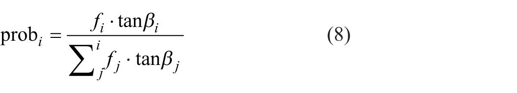
Where i is the currently processed neighbor cell and j represents all neighbors in set N, the weighting factor f equals the persistence factor p (with p ⩾ 1) if the flow direction to neighbor i matches the previous direction, otherwise f = 1. This persistence factor increases the likelihood of selecting the neighbor in the current flow direction, reducing abrupt changes. Transition probabilities, weighted by slope, are normalized between 0 and 1, and one cell is then randomly selected from the set N using a pseudo-random generator.

The slope threshold allows the model to adapt to different terrain types by restricting steep-flow paths in steep areas and allowing more divergent flow in flat areas. This regulation, controlled by an exponent, is a key feature missing in hydrological models that distribute flow proportionally among all lower neighbors without considering local topography.

For the parameterization of this model, the same digital elevation model used in previous cases was employed, along with raster-format seeds indicating the areas from which landslides initiated, like what was used for Flow R, and the friction angle in vector format for the soils present in the basin.

In the landslide model setup, two approaches can be chosen for flow direction: unidirectional, which selects the cell with the lowest height, or the Random Walk method, which considers multiple directions and is sensitive to local slope (Wichmann, 2017). Most simulations utilized Random Walk, while the unidirectional approach was used solely for validation.

To calculate “runout” (the distance traveled by a particle), three energy-based options are provided: geometric gradient, Fahrboeschung, and shadow angle, each with different methods for defining vertical and horizontal distances. Friction models with either one or two parameters can also be employed, such as the PCM model originally designed for avalanches.

For the GPP, input parameters selected included the digital elevation model, scarps, and friction angle. Although this application allows for many other parameters in its analyses, it was decided to use only those that are also accepted in other applications to maintain simplicity in modeling and ensure that comparisons between results are based on the same information as possible. Table 5 shows the values of the variables considered in the different simulations.

Table 5.

Setup of executed tests in SAGA GIS with GPP module.

Simulation	1	2	3	4	5	6	7	8	9	10
Input parameters	1	1	1	1	1	1	1	1	1	1
Model	RW	RW	RW	RW	RW	MS	MS	MS	MS	MS
Runout model	GG	F	SA	PFM	PCM	GG	F	SA	PFM	PCM
Slope threshold [%]	-	-	-	-	-	-	-	-	-	-
Simulation	11	12	13	14	15	16	17	18	19	20
Input parameters	1	1	1	1	2	2	2	2	2	2
Model	RW	RW	RW	RW	RW	RW	RW	RW	RW	RW
Runout model	GG	F	SA	PFM	PCM	GG	F	SA	PFM	PCM
Slope threshold [%]	45	45	45	45	45	40	40	40	40	40
Simulation	21	22	23	24	25	26	27	28	29	30
Input parameters	2	2	2	2	2	2	2	2	2	2
Model	RW	RW	RW	RW	RW	RW	RW	RW	RW	RW
Runout model	GG	GG	GG	GG	GG	GG	GG	GG	GG	GG
Slope threshold [%]	20	25	30	21	22	23	24	26	27	28
Simulation	31	32	33	34	35	36	37	38	39	40
Input parameters	2	2	2	2	2	2	2	2	2	2
Model	RW	RW	RW	RW	RW	RW	RW	RW	RW	RW
Runout model	GG	GG	GG	GG	GG	GG	GG	GG	GG	GG
Slope threshold [%]	25	26	27	28	30	20	20	20	20	20

Results

The modeling processes referred to in Tables 2, 4, and 5 were conducted. With these results, a similarity analysis was performed against the records of the event on May 18, 2015, in the La Liboriana basin, and the case with the highest graphical similarity was selected considering area similarities. In this regard, the results obtained for RAMMS, Flow R, and the GPP are presented for each model, along with analyses of the input parameters and their impact on the results.

Furthermore, the primary criteria for selecting the best model for each application was its graphical similarity with the landslide analyzed in the La Liboriana case study and then with the calibrated parameters it was applied in the La Argelia case. The results for each evaluated case are presented below.

La Liboriana Basin

All results obtained for each application were reviewed, and the one that appeared to best replicate both the shape and length of the real case landslides was chosen.

Flow R

According to the executed models (see Table 2), multiple results were obtained. However, the objective of conducting these simulations was to find the optimal combination of parameters and algorithms that could accurately simulate the events that occurred in the selected case study. In this context, not all results achieved this goal and therefore had to be discarded.

Those results that met the selection criteria were re-analyzed among themselves and reviewed again to select the one that most closely resembled reality.

After analyzing the models and their results, it was found that Model 19 provided the best outcomes based on the graphical correspondence between the actual landslides and the simulated ones. Actual landslides occupy an area of 0.37 km² and the ones estimated with Flow R occupy 0.65 km². The results of this model are shown in Figure 6.

Figure 6.

Simulation results for the calibration case using Flow-R with parameter combination #19. The map shows the modeled landslide propagation probability, overlaid with observed landslides and stream networks.

For the execution of the simulations the modified Holmgren algorithm was implemented, configuring a dh of 0.005 and a value of x = 25, which improved flow dispersion by adjusting the height of the cells and their relationship with neighboring cells.

The model was set up using the “Quick” calculation method, allowing for a rapid and progressive assessment of the source cells. Flow inertia was calculated by assigning weights through the Gamma function, prioritizing the previous flow direction and preventing backflow. During sensitivity analysis, values of xx between 1.0 and 25.0 were tested, discarding lower values due to extensive divergences, concluding that 15.015.0, 20.020.0, and 25.025.0 produced similar results.

RAMMS

For each run performed with RAMMS, the same digital elevation model (DEM), the corresponding layer of seeds where the recorded landslides initiated in the case study, and the height of the sliding layer calculated from the previously described methodology were utilized.

Variations in these simulations focused on the values of the soil viscosity friction parameter ( $\mu$ ) and the drag coefficient ( $\xi$ ). The density for these simulations was consistently set at 2,000 kg/m³, as this is an acceptable value for the type of soils considered in these simulations according to literature. In Figure 7 the results of the maximum values of height, speed, and pressure are observed.

Figure 7.

Simulation results for the calibration case using RAMMS with parameter combination #24. (A) Maximum height [m]. (B) Maximum velocity [m/s]. (C) Maximum pressure [kPa]. Observed landslides and streams are shown for reference.

In summary, the results obtained from RAMMS correspond to the maximum flow deposition height, maximum flow velocity developed during its trajectory, maximum pressure, and maximum momentum. However, the latter result was not considered for this research as it does not relate to the outcomes obtained with other applications used. The model that provided the best results, in graphical terms, corresponds to Model 24 (see Table 4) where the estimated landslides occupy an area of 0.85 km².

Regarding these results, it can be observed in Figure 6 that the maximum depth obtained in the deposition areas of the flow corresponds to a height of 1.5 m, occurring only in areas where the flow likely encountered obstructions in its path. In the remaining sections of each landslide scarp, low heights, on the order of 10 cm or similar values, were identified.

As shown in Figure 2B, slopes between 50° and 78° are identified, which are considerably high values, indicating very steep terrain; thus, depths of 10 cm of flow could even be considered excessive given this context. This is also closely related to the time it may have taken for the landslides to occur and transport material to their final deposition site. However, time is not within the scope of this research, so this concept is not explored further.

GPP

Regarding the GPP module of SAGA GIS, the result obtained is the delineation of a landslide trajectory. The model setup involved the digital elevation model (DEM), scarps, and friction angle as parameters. Analyses were conducted using the Random Walk model with runout measurement based on a single-parameter friction model. Additionally, the soil friction angle was incorporated as a layer.

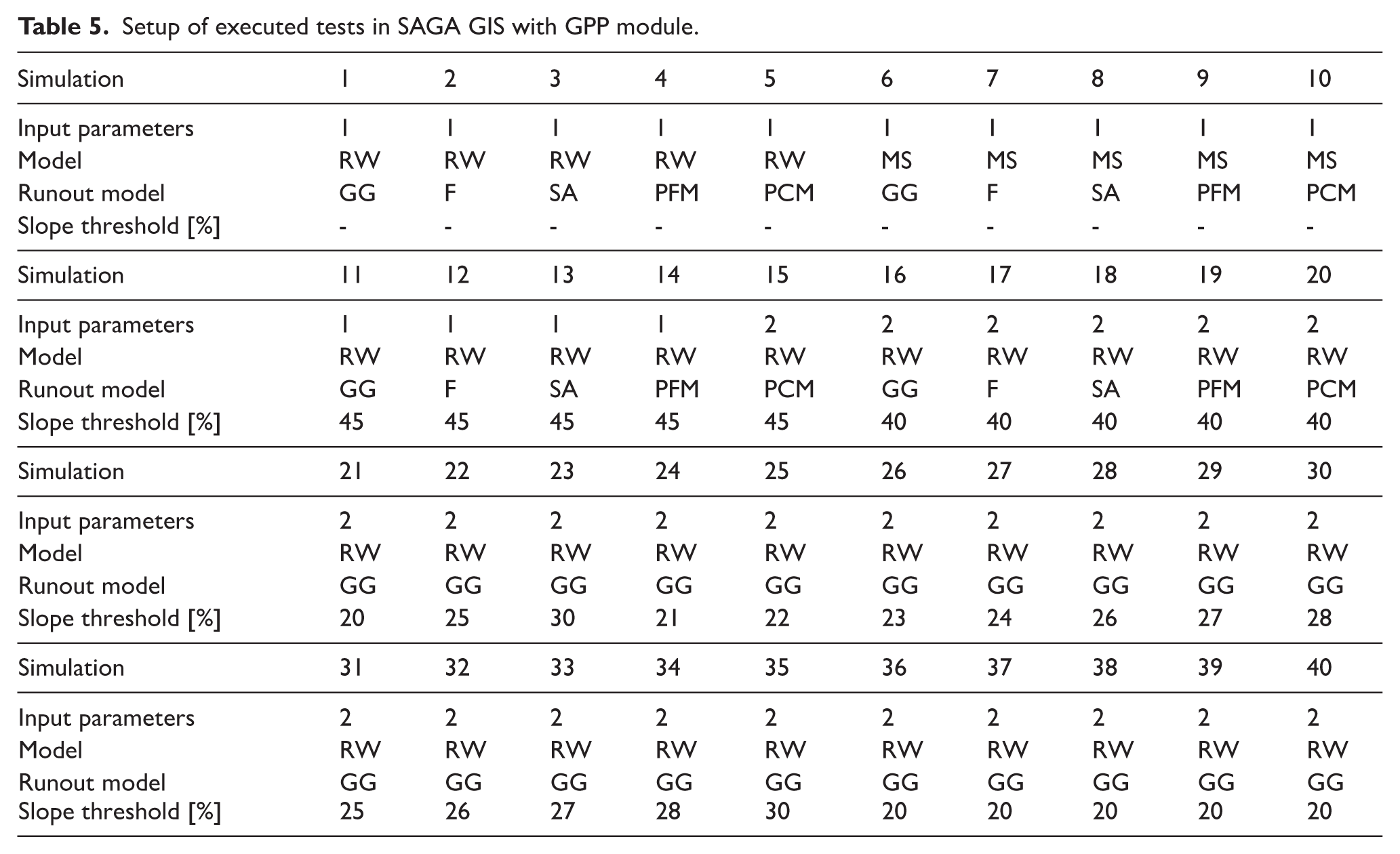
Concerning the results obtained and considering the combinations used for the simulations, the model that provided the best graphical results corresponds to Model 36, where the estimated landslides occupy an area of 1.11 km². The results of this model are shown in Figure 8. As observed, the results yield values ranging from 0 to 96,078. This indicator reflects the frequency of how many times a cell was traversed.

Figure 8.

Simulation results for the calibration case using GPP with parameter combination #36. The map displays the modeled distribution of landslide runout intensity, expressed as the number of cells affected.

As previously mentioned, the outcomes from this application correspond to the propagation of the landslide under specific parameters and the runout or extent of the landslide.

With the algorithms employed for executing the simulations, it was possible to control the degree of flow divergence; thus, calibration focused on finding the optimal combination that maintained a balance between divergence and convergence of flow while simultaneously reproducing an event like that analyzed in the case study.

During the analysis process for the development of the simulations, it was identified that the best model performance occurred for slopes below 20%. For this reason, a slope threshold of 20° was adopted, allowing landslides to occur only in areas with slopes under this limit. However, this does not reflect the actual slope conditions of the watershed, as shown in Figure 3, where slopes of 45° or more are present, particularly in zones where scarps are located. For steeper slopes, the model was unable to reproduce the landslides that occurred, even when adjusting the level of divergence allowed by the algorithm. This limitation represents an important consideration within the main conclusions of this exercise.

La Argelia Basin

As mentioned, for the validation case, the models with the parameters and setups determined to be optimal during the calibration stage were used. The results obtained with each of the applications are presented below.

Flow R

The results obtained with this application reflect divergent flows, as shown in Figure 9. However, it is evident that within the polygons of the actual landslides, in most cases, the probability of propagation is highest, indicating that the application predicts a 100% likelihood of a landslide occurring in those areas. This serves as a guarantee that an event indeed took place in those zones, regardless of the level of overlap with the polygons obtained. The estimated landslides occupy an area of 1.12 km², while the real landslides occupy an area of 0.44 km².

Figure 9.

Simulation results for the validation case using Flow R.

RAMMS

As can be seen in Figure 10, while volumes of material are displaced from the indicated areas where landslides initiate, it is noticeable that in no case do they achieve a trajectory long enough to reproduce the landslide itself. The estimated landslides occupy an area of 2.08 km², while the real landslides occupy an area of 0.44 km². This is particularly true in cases where the polygons are very small, raising doubts about whether the results obtained at these specific points are accurate or merely a reflection of the scar size.

Figure 10.

Simulation results for the validation case using RAMMS: (A) Maximum height [m], (B) maximum velocity [m/s], and (C) maximum pressure [kPa].

The comparison of the results obtained during the calibration of the model with the La Liboriana River basin indicates that the model may need to be calibrated for each specific case. In that instance, it is evident that the trajectories followed by the flows are more like the actual landslide footprints that occurred.

Regarding the magnitudes of the results obtained, it makes little sense to compare them with those from the calibration since they involve two different basins with clearly distinct topography and varying proportions of steep slopes. Additionally, since this basin is not instrumented and lacks information on past events, there are no records available to compare against the values obtained for depth, velocity, and pressure.

This situation applies to all evaluated parameters (deposition height, velocity, and pressure). Therefore, it is necessary to modify the viscosity since the results suggest that the mass is not sufficiently fluid to flow downhill in most cases, particularly in the upper part of the basin, where, as shown in Figure 2B, many of the highest slopes in the entire study area are developed, with values ranging between 50° and 70°.

GPP

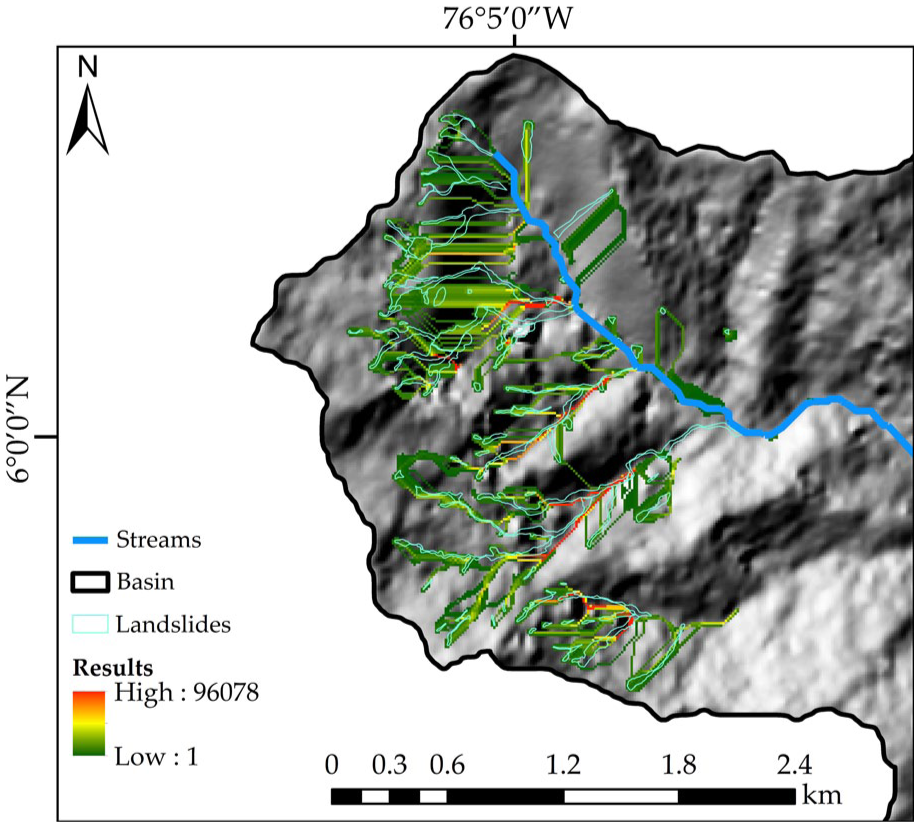
The same model selected for the calibration case was executed. The results obtained are presented in Figure 11. The estimated landslides occupy an area of 1.13 km², while the real landslides occupy an area of 0.44 km². The results show the trajectories of the landslides extending to the watercourses present in the basin. There is no relationship with the rheological parameters of the mixture, meaning there is no connection to viscosity or similar factors as seen in RAMMS. The application only indicated the flow direction of the mixture from the initiation cells of movement. However, the way the flow spreads according to this result is much more divergent than in reality. Some landslides can be noted where the results closely resemble the footprints from the inventory, particularly in the lower part of the study area. However, this is not a generalized finding, as in the upper landslides and central zone, the flow diverges significantly, resulting in trajectories that are much broader than those followed by the studied landslides.

Figure 11.

Simulations results for the validation case using GPP.

While the model reproduces events to some extent, it is evident that further calibration is necessary by adjusting the parameters controlling flow divergence within the selected algorithm of this module. This adjustment should encourage the flow to follow a more defined and unidirectional path, consistent with the patterns exhibited by real landslides.

Analysis and Validation

To analyze the results of the models for both basins, a graphical comparison was initiated between the actual landslides and those obtained in the simulations for the calibration case. In the case of RAMMS for the La Liboriana basin, it was observed that the simulations matched the footprints of the landslides in the upper initiation zones but failed in the deposition areas, showing an affected surface of 0.85 km², which is 2.3 times greater than the actual area of 0.37 km². Flow R produced landslides over an area of 0.65 km² (1.75 times larger), while GPP indicated an area of 1.11 km² (three times more). Although all three models overestimated the affected areas, Flow R was closest to the actual magnitude of affected areas, with GPP showing 55% coincidences, followed by RAMMS at 40% and Flow R at 34%.

RAMMS exhibited limitations by concentrating on landslides in initiation zones without extending downstream. The lack of a stratigraphic profile and reliance on assumed soil depths (maximum 2.5 m) generated uncertainty, limiting the simulated material volume and affecting flow reach.

For Flow R, changes in slope did not significantly impact runout, as in some cases landslides extended beyond actual limits, while in others, they followed terrain contours. It was noted that trajectories on lower slopes matched real ones, whereas on steeper slopes, such as Cerro Plateado, parallel trajectories were detected. This pattern also appeared in GPP results from SAGA GIS.

This analysis highlights that while RAMMS has limitations due to viscosity values and lack of detailed data, Flow R and GPP provide good results but with a margin of overestimation due to their risk analysis nature.

Regarding results for the La Argelia River basin, it has been observed that while calibrating models with the La Liboriana River basin laid the groundwork for using applications in other basins with similar characteristics, the quality of results obtained is not comparable graphically. There is a clear difference between results from the first basin and those from the second. Although it is evident that results are not unrelated to actual events, they do not adequately reproduce conditions in the La Argelia River basin. This discrepancy may stem from significant differences in rheological parameters between the two basins. They do not behave identically during sliding or when movement energy dissipates. Additionally, topography and slope setups directly affect these processes and consequently influence results; thus, establishing analysis thresholds within direction algorithms must be done specifically for each condition being evaluated.

However, from the previous analysis alone, it is not possible to measure the performance of each application since it only addresses a qualitative evaluation of obtained results. Therefore, methodologies were sought to allow for quantitative evaluations that could also be statistically analyzed. To achieve this, it was determined that raster files containing simulation results should be unified into a single value indicating whether a landslide occurred or not. Specifically, all rasters were converted so that cells where landslides were recorded were assigned a value of one (1), while those where no landslide occurred were assigned a value of zero (0).

Since the objective is to perform a binary analysis of the results, an error analysis was performed, the results of which are shown in Table 6. Initially, the root mean square error (RMSE) was used to evaluate the cells of the raster files containing the results and quantify the prediction error in terms of units calculated by the model during calibration. The RMSE index is given by the following equation.

$$\mathrm{RMSE}=\sqrt[2]{\frac{{{\displaystyle \sum }}_{i=1}^N{(0_i-P_i)}^2}{N}}$$

(9)

Where $0_i$ and $P_i$ represent the sample of size N. N corresponding to the observations and model estimates. The expected result varies between 0 (zero) and 1 (one), where values close to zero indicate a perfect fit of the model according to the obtained experimental data (Ritter & Muñoz-Carpena, 2013).

Additionally, a third goodness-of-fit indicator was calculated, represented by the equation shown below, which is an efficiency coefficient that is the complement to one of the ratios between the mean squared error of the observed values against the modeled values and the variance of the observations (Ritter & Muñoz-Carpena, 2013).

$$\mathrm{NSE}=1-{\left(\frac{\mathrm{RMSE}}{SD}\right)}^2$$

(10)

Where SD corresponds to the standard deviation of the results obtained with each of the applications. Based on this, it is possible to verify the goodness of fit of the model obtained concerning the simulations executed through the relationship between SD/RMSE and the values obtained for NSE (Nash-Sutcliffe Efficiency), as seen in Table 6.

Table 6.

Results of the performance of the applications with RMSE.

Applicative	RMSE	NSE	SD/RMSE	Performance
Flow R	0.3288	−0.0293	0.9856	Low
GPP/SAGA GIS	0.3287	−0.0989	0.9536	Low
RAMMS	0.3136	−0.2478	0.8952	Low

The results of the goodness and performance evaluation of the model showed low values, despite the root mean square error being close to zero. This is because the evaluation excessively penalizes results based solely on exact matches between predictions and reality, without considering whether the model approximately reproduces the phenomenon. This approach does not integrate qualitative analyses and focuses solely on the accuracy of the match with the comparison data, which may lead to dismissing the applicability of the models. Furthermore, factors such as digitization accuracy, data sources, or soil parameters like viscosity, which influence the results, are not considered.

Due to the limitations of the previous metrics, an additional analysis was conducted to evaluate whether there were false predictions in areas close to the cells where landslides occurred. The ROC (Receiver Operating Characteristic) curve was used, a statistical tool that classifies cells into two groups: those that present the event of interest (landslides) and those that do not, providing a more comprehensive assessment of model performance.

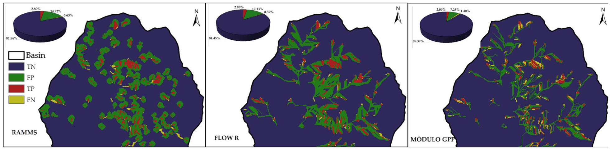
The cells from the results of RAMMS, Flow R, and the GPP module were classified into four categories: true positive (TP), true negative (TN), false positive (FP), and false negative (FN), based on the confusion matrix from the ROC analysis. From this, the true positive rate (TPR) and false positive rate (FPR) were calculated. The results of the consistency matrix are shown in Figures 12 and 13 for the La Liboriana and La Argelia basins, respectively, and Figure 14 shows the ROC curves.

Figure 12.

Confusion matrix for La Liboriana basin: (A) Flow R, (B) RAMMS, and (C) GPP.

Figure 13.

Confusion matrix for La Argelia basin: (A) Flow R, (B) RAMMS, and (C) GPP.

Figure 14.

Receiver operating characteristic (ROC) curves for model calibration (left column) and validation (right column).

For the La Liboriana basin, Flow R achieved a True Positive Rate (TPR) of 35% and a False Positive Rate (FPR) of 5%, reflecting reasonable matches with the footprints of actual landslides. RAMMS showed a TPR of 33% and an FPR of 7%, similar to Flow R. The GPP module performed best with a TPR of 56% and an FPR of 8%, indicating the highest correspondence with the real case. All models exhibited similar error rates.

In the case of the La Argelia basin, the results indicated True Positive Rates (TPR) of 13% for Flow R, 15% for RAMMS, and 7% for the GPP module of SAGA GIS. Regarding False Positive Rates (FPR), Flow R had 83%, RAMMS 82%, and GPP 59%. These results suggest that models calibrated for the La Liboriana River basin did not correlate well with the landslide inventory from the La Argelia River basin. Compared to the study case, the rates in this basin were significantly lower for TPR and much higher for FPR, indicating that the models produced more inaccuracies in this basin.

It is important to mention that the only information available for this validation is the extent, as can be compared with the results from the landslide inventory found in the literature. For the other parameters, there are no field records that allow for more complete and detailed validation.

The area under the curve (AUC) was calculated for each of the ROC curves to evaluate the performance of the models, as a higher AUC value indicates better performance. The results were as follows: Flow R with an AUC of 0.658, RAMMS with 0.632, and GPP with 0.615. This shows that, in general, Flow R demonstrates the best performance among the three evaluated models according to this metric. The obtained AUC values are considered conservative or acceptable, with similar results found in other studies, which will be discussed later.

In analyzing the ROC curves for the models applied to the La Argelia River basin, the areas under the curve (AUC) were calculated to assess their performance. The results were as follows: GPP from SAGA GIS with an AUC of 0.60, RAMMS with 0.57, and Flow R with 0.59. Compared to the results from the La Liboriana River basin, these values are relatively close, but RAMMS and Flow R are below 0.60, suggesting that the models may require better calibration for this specific basin.

Overall, for La Liboriana basin, Flow R showed the best performance with an AUC of 0.658, followed by RAMMS at 0.632 and GPP at 0.615. These values are considered conservative or acceptable and reflect that while the models have similar areas under the curve in both basins, Flow R’s performance was superior. However, the AUC values for La Argelia indicate that RAMMS and Flow R may need additional adjustments to improve their accuracy in that basin.

Furthermore, based on this analysis, three confusion maps were constructed, one for each application, to visually observe where matches occurred and where false predictions were generated. The results of the consistency maps are shown in Figures 15 and 16 for the La Liboriana and La Argelia basins, respectively.

Figure 15.

Spatial confusion maps for La Liboriana basin.

Figure 16.

Spatial confusion maps for La Argelia basin.

The analysis of the confusion maps reveals that the RAMMS model shows a good match with areas where no landslides occurred (true negatives, TN), but it presents many false positives (FP), predicting landslides in zones where they did not occur. However, the model largely identifies actual landslides, although it tends to overestimate their extent.

For the GPP module, the majority class is TN. Although true positives (TP) have a higher percentage of matches compared to RAMMS, there is no clear pattern of actual landslides identified. This module also shows many FP, likely due to its flow direction analysis.

Regarding the Flow R model, it also tends to overestimate landslides but can reproduce most actual landslides. While the match percentages are low compared to other classes, this is because 97% of the cells do not show landslides in the real case, and only 3% correspond to actual landslides. Thus, the true positives obtained are proportional to the real landslide areas.

In the analysis of confusion maps for the La Argelia basin, significant differences were observed compared to the results from the La Liboriana basin.

For RAMMS in La Argelia, a good match was noted with areas without landslides (TN), but there was many false positives (FP), predicting landslides in zones where they did not occur. Despite overestimation, the model managed to identify a substantial portion of actual landslides.

In the GPP module, most cells were classified as TN, with a higher percentage of true positives (TP) compared to RAMMS, though without a clear pattern. Like RAMMS, GPP exhibited many FP, likely due to its flow analysis.

For Flow R, there was an observed overestimation of landslides, but the model correctly identified most actual landslides. Despite low match percentages compared to other classes, these accurately reflect the real proportion of cells with landslides in the La Argelia basin.

In summary, although the models exhibited overestimation and many false positives in both basins, the La Argelia basin showed patterns and match rates like those observed in La Liboriana, with differences in identification capability and precision for each model.

Discussion

The results show that Flow-R was closest to the actual magnitude of affected areas, with 34% coincidences. This performance aligns with previous studies that have confirmed the capabilities of this software. In the Flow-R study conducted by Nie et al. (2022), a 12.5 m DEM from the ALOS PALSAR mission was used, along with flow accumulation data, slope, curvature, and land use data. They validated results using a list of 89 landslide points, predicting 78 of them, yielding an accuracy of 87.6%. Although this analysis measures landslide occurrence prediction without considering exact matches between actual and predicted extents, it conclusively demonstrates the tool’s utility. Additionally, no further analysis was needed for cells where landslides initiate since the inventory was based on satellite imagery. The methodology employed in other research, such as (Pastorello et al., 2017), could be useful in cases where an adequate inventory does not exist; different flow-divergence parameter values were used to refine results case-by-case.

On the other hand, the results show that with secondary information, using these tools is feasible at low cost for areas with scarce data, unlike other studies relying on primary data. For example, all applications used a digital elevation model from the ALOS PALSAR satellite mission at 12.5 m resolution. In other studies where these applications modeled previous events (Cesca & D’Agostino, 2008; Díaz-Salas et al., 2021; Franco-Ramos et al., 2020), terrain information was collected by more precise methods such as LiDAR, providing primary data about the real and current terrain where events occurred. Here, the first factor leading to reduced precision in predictions was the use of derived parameters from the digital elevation model, like slope, aspect, curvature, and flow accumulation for Flow-R.

That being the case, the spatial resolution of a Digital Elevation Model (DEM) influences landslide propagation modeling by affecting the accuracy of terrain parameters, which are essential for identifying initiation zones and flow paths. Studies have shown that DEM-derived attributes such as slope, curvature, and drainage network are strongly dependent on spatial resolution (Dai et al., 2025; Shafique et al., 2011). Moderate-resolution DEMs (around 10–12.5 m) can effectively capture detailed terrain variability, preserving sharp slopes, microtopographic features, and subtle curvature contrasts, which improves hazard delineation and model sensitivity (Chang et al., 2019; Meena & Gudiyangada Nachappa, 2019). Conversely, coarser DEMs tend to smooth these terrain attributes, underestimating slope steepness and reducing curvature variability, leading to less precise identification of vulnerable areas (Dai et al., 2025; Shafique et al., 2011). This smoothing effect also impacts channel depiction and flow direction allocation, since fine-resolution DEMs allow precise mapping of drainage networks and flow convergence zones, enabling more realistic flow routing (Qiu et al., 2022). However, excessively fine DEMs may introduce noise and artifacts that disrupt flow-path prediction unless appropriate noise filtering is applied (Qiu et al., 2022). Therefore, selecting an optimal DEM resolution that balances terrain detail and noise minimization is crucial for robust landslide modeling. Future research into the assessment of these effects should also be extended to other areas where high-quality topographic data is available.

Regarding RAMMS performance, it ranked second in performance with 40% coincidences. This is attributable to the complex nature of the modeled phenomenon and scarcity of rheological data, especially since this study used parameters obtained from secondary sources. Regarding soil rheological parameters, no information existed about the soils involved in the analyzed events. No viscosity records were found, and friction parameters were generalized from literature aligned with regional geology. Specifically, viscosity and viscous-turbulent friction values suggested in the RAMMS user manual were used. In contrast, Hussin et al. (2012) used values from well-instrumented, similar basins, yielding high-quality data. Nonetheless, literature values were expected to still reflect real cases. Cesca and D’Agostino (2008) in a similar comparison of RAMMS with Flo-2D (unavailable here), used turbulent friction factors ξ ranging from 15 to 1,000 m/s² based on literature, selecting 1,000 m/s² for this study. For example, other studies used 0.05 and 1,200 m/s² in the Swiss Alps (Frank et al., 2015); 0.15 and 400 m/s² with density 1,400 kg/m³ at Pico de Orizaba volcano, Mexico (Franco-Ramos et al., 2020); and 0.12, 1,000 m/s², and 1,000 kg/m³ in a Peruvian Andes sub-basin case. While viscosity values vary between studies, viscous-turbulent friction coefficients hover around 1,000 m/s² in alpine and Andean regions, suggesting RAMMS output sensitivity is greater for viscosity than friction coefficients.

The dependence on literature-derived rheological parameters in RAMMS, as well as the need to adopt default slope-threshold settings in GPP, reflects a broader limitation inherent to tropical data-scarce environments. Without field-based measurements of soil strength, rheology, or hydrological response, viscosity, turbulent friction, and soil-depth assumptions must be taken from studies in comparable Andean or alpine contexts, providing a defensible yet uncertain starting point for model operation. Likewise, the GPP model’s requirement to impose a 20° slope threshold, which contrasts sharply with the predominance of >45° slopes in both basins, reveals a structural mismatch between the model’s original design conditions and the geomorphological realities of steep tropical catchments. Together, these limitations highlight the high sensitivity of landslide-propagation models to rheological and geometric controls and underscore the need for future work integrating basin-specific soil testing, sensitivity and uncertainty analyses, and adaptive calibration frameworks to better represent steep tropical terrains.

GPP ranked third in performance, with 55% coincidences. Goetz et al. (2021) used a Random Walk model for lateral runout dispersion and noted that many landslide trajectories at edges matched those herein. They also cautioned that DEMs with resolutions coarser than 20 m may oversimplify smaller rills and flow accumulation, and the 12.5 m DEM used might have been resampled from higher resolution sources. Despite this, the results effectively modeled real conditions and potential flow paths, identifying susceptible landslide zones.

Regarding soil sliding-layer depth, two considerations arose due to the calculation equation: slopes above 45° were set constant, as soil formation is assumed absent on steeper slopes; slopes at 0° were adjusted to avoid division by zero. Ortiz et al. (2023) applied the same expression along Ovejas Creek banks, obtaining depths of 0.51 to 1.5 m for medium to high slope zones comparable to values found here. Without stratigraphic profiles, limiting depth to 1.5 m constrains displacement volume and flow reach.

Though parameters exhibit high spatial variability impacting quality, simulated landslides in La Liboriana basin showed acceptable consistency with actual polygons, albeit with some positional offset. In contrast, results in La Argelia basin exhibited less concordance, likely due to limited data from this sparsely populated rural region with low economic impact and thus less monitoring.

The decline in performance when parameters calibrated in La Liboriana were applied to La Argelia, exhibited by true positive rates dropping to 7% to 15% and false-positive rates exceeding 80%, reveals the limited transferability of landslide-propagation models across basins with markedly different physical environments. Contrasts in lithology, soil mechanical behavior, slope distribution, vegetation cover, and roughness significantly influence both initiation and runout processes, making a single parameterization insufficient for both basins. La Argelia’s dominance of very steep slopes (>50°), highly fractured volcanic rocks, and extensive forest cover produces landslide dynamics that differ substantially from the sedimentary, agriculturally modified La Liboriana basin. These results align with earlier findings that transferable automated modeling in tropical mountainous regions remain challenging, and underscore the need for basin-specific calibration, expanded local data collection, and adaptive parameterization frameworks to reduce systematic bias and improve prediction accuracy across heterogeneous Andean landscapes.

Overall, the models achieved ~60% coincidence between landslide areas and inventory polygons, with AUC values near 0.6 considered acceptable or conservative (Pradhan & Kim, 2016), supporting model efficacy despite data and spatial uncertainties. Similar AUC results were reported by Hidalgo and Vega (2021) for probabilistic landslide risk in La Liboriana, alongside other regional studies with AUCs from 0.56 to 0.8 (Marin et al., 2021; Ruiz-Vásquez & Aristizábal, 2018), validating comparability despite methodological differences.

The relatively low RMSE and NSE values must be interpreted considering uncertainties in the reference inventory, which was digitized from satellite imagery and inherently contains spatial approximation errors. RMSE and NSE remain widely accepted for geomorphological modeling, but their sensitivity to mismatch between modeled and observed extents reflects both model limitations and uncertainties embedded in historical outlines. This interaction between model performance and observational uncertainty is well documented in data-scarce settings. Within the scope of this work, focused on comparing model behavior under consistent conditions, these metrics provide an internally coherent and methodologically sound evaluation framework, while more advanced probabilistic or uncertainty-quantification approaches are identified as directions for future research.

In general, low ROC values in landslide propagation modeling imply that the models reflect the reliance on secondary data sources, insufficient field-based calibration of critical geotechnical and topographical parameters, and the use of moderate-resolution DEM. In addition, the landslide inventory used for model validation was generated from remote sensing and image interpretation, introducing further uncertainty. These low ROC values reflect the conservative and preliminary nature of the hazard assessment in tropical, data-poor mountain basins.

In other RAMMS and Flow-R studies, calibration used detailed event data (displaced volumes and runout) for model-accuracy assessment (e.g. Hussin et al., 2012). Such detailed data was unavailable here, particularly due to the inventory’s size, making similar analyses inapplicable.

Finally, a marked difference exists between our calibration basin (La Liboriana) with abundant documentation and the less-studied La Argelia basin, where forest covers, sparse habitation, and few roads limit landslide reporting.

Conclusions

The comparative analysis of the RAMMS, Flow-R, and GPP models using secondary data indicates that despite their generally conservative performance, these models yield acceptable and regionally comparable results in simulating landslide runout distances. This supports their use as valuable tools for hazard evaluation in data-scarce Andean tropical regions such as rural Colombia. Among the three, Flow-R demonstrated superior overall predictive performance, followed by RAMMS, with GPP ranking third. RAMMS showed limitations by concentrating predicted landslides primarily near initiation zones, often underrepresenting downstream propagation. These constraints stem largely from its viscosity assumptions and the scarcity of detailed calibration data, whereas Flow-R and GPP, while potentially overestimating affected areas due to their probabilistic frameworks, offer reliable outputs for preliminary risk assessments.

Calibration in the La Liboriana basin establishes a methodological foundation for applying these models to similar basins such as La Argelia. Although model outcomes generally align with observed landslide events, discrepancies persist, likely attributable to spatial heterogeneity in rheological, topographic, and land cover parameters. Data quality challenges, including incomplete inventories and dated satellite imagery, further complicate hazard assessments in Colombia. Nonetheless, the models provide valuable conservative approximations of potential sliding scenarios to aid decision-making.

Looking forward, future research could enhance predictive capability by integrating detailed rainfall hydrographs across various return periods to estimate event probabilities, as well as incorporating additional terrain parameters to improve model fidelity. Similarly, future work will focus on expanding the evaluation of the effect of each model’s parameterization and assessing how the spatial resolution of the DEM affects slope and curvature smoothing, channel depiction, and flow direction allocation.

Among the three evaluated models, Flow-R is best suited for regional-scale susceptibility mapping, offering efficient identification of potential source areas and hazard propagation over broad, complex landscapes. RAMMS excels in detailed event-scale simulations, particularly channelized debris flows, requiring comprehensive parameterization and software licensing, making it ideal for precise hazard zoning and engineering applications. GPP provides a rapid, open-access option for preliminary hazard delineation under data-scarce conditions, trading some physical details for accessibility and ease of use.

Recommended parameter ranges for the tropical Andean context include Voellmy friction coefficients (μ) between 0.1 and 0.2 (reflecting the most observed values un previous RAMMS calibrations; Mikoš & Bezak, 2021) and turbulent friction coefficients (ξ) of 200 to 500 m/s² for RAMMS, and slope thresholds near 20° for GPP to mitigate unrealistic flow divergence from DEM noise. Model performance metrics like AUC, TPR, and FPR align with regional conditions but vary with data quality and terrain complexity. Applicability limits stress the need for DEM resolution around 12.5 m or less, detailed landslide inventories for calibration, and software accessibility considerations, enabling users to match model choice with study objectives, data availability, and practical constraints.

Critical to practical application, two of the three evaluated models (GPP and Flow-R) are freely available and user-friendly, facilitating rapid deployment for governmental and non-governmental agencies. This accessibility lowers technical barriers, enabling incorporation into landslide early warning systems, regional risk management, land use planning, and emergency response. Moreover, the methodology can be extended to vulnerable areas without recent landslide history, supporting proactive, anticipatory risk analyses. Given its relative simplicity and replicability, this approach can help inform evidence-based decisions across diverse Andean contexts.