Sage Journals: Discover world-class research

Abstract

Anthropogenic environmental pollution is a known and indisputable issue, and the importance of searching for reliable mathematical models that help understanding the underlying process is witnessed by the extensive literature on the topic. In this article, we focus on the temporal aspects of the processes that govern the concentration of pollutants using typical explanatory variables, such as meteorological values and traffic flows. We develop a novel technique based on multiobjective optimization and linear regression to find optimal delays for each variable, and then we apply such delays to our data to evaluate the improvement that can be obtained with respect to learning an explanatory model with standard techniques. We found that optimizing delays can, in some cases, improve the accuracy of the final model up to 15%.

Keywords

Time series explanation multiobjective optimization lagged linear and nonlinear regression

Introduction

Anthropogenic environmental pollution is a known and indisputable issue. Every day, the human body is exposed to harmful substances in various ways, including by ingestion of food and drink and by absorbtion with breathing. While it is possible to limit the ingestion of harmful chemicals, it is impossible to choose the air we breathe. Chemicals dangerous to health (or that become so if absorbed over certain amounts) include suspended particulate matters, nitrogen oxides, $C O$ , and $S O_{2}$ . Exposure to these pollutants adversely affects human health, as confirmed by numerous scientific studies conducted in recent years around the world: Poland,^1,2 Deutschland,³ Italy,⁴ USA,^5-7 Canada,⁸ Australia,⁹ Chile,¹⁰ among many others. While the quality of air is usually regularly monitored, actions leading to the reduction of air pollution are most definitely a growing need. Generally, anthropogenic sources of air pollution are known, and, due to the development of civilization, it is impossible to completely eliminate them. Therefore, scientific studies are conducted to determine the impact of factors that modify their concentrations via transformation, retention, or evacuation, and, to this purpose, mathematical models are an essential tool. Recognizing the factors that have the greatest impact on the concentration of pollutants in the air at a certain moment gives the opportunity to build plans for their manipulation, when possible, or, at least, for the improvement of design of cities, streets, crossroads, and houses, to ensure the fastest possible evacuation of contaminants, shorten the time of exposure to its harmful effects, and reduce the intensity of their action. In general, such models are known as land use regression models—LUR (see previous studies,^11,12 among many others). However, in addition to the identification of the factors themselves, the timing of their effect also plays a significant role. For example, a momentary gust of wind results in a much smaller evacuation of pollutants than a wind with the same speed persisting for several hours. Therefore, it is important to identify not only the factors in play, but also the moment in time in which their influence on the concentrations of pollution is the greatest, to obtain a temporal land use regression model (TLUR).

Predicting the value of a time series, such as the concentration of a certain pollutant in time, is a very well-known problem. The usual statistical approach to its solution requires the use of moving average models, or, more generally, of Autoregressive Integrated Moving Average (ARIMA) models, that define the problem as an autoregressive one (see Box et al¹³ for a comprehensive introduction). The underlying idea is that the past values of the predicted variable, for example, the pollution concentration, can be used to predict future values. The implicit assumption is that the behavior of the predicted variable remains somewhat constant, and such models are designed to identify, and describe, such behavior. A different approach, more typical of machine learning, consists of enhancing a static model learner (eg, linear regression, tree regression, neural network) with lagged variables, that is, variables with the past values of the predictors. A classical regression model is designed to extract a (implicit or explicit) function of the (current) predictors that explains the (current) value of the interesting variable; a lagged regression model acts in the same way, but using, as predictors, both the current and the past values of the explanatory variables. The so-called ARIMAX models mix these 2 ideas, and are designed to extract functions of both the current and past values of both predicting and predicted variables. The most relevant drawback of ARIMA-type frameworks is that the resulting models are, in a way, implicit. As a matter of fact, in most natural phenomena, the variable to be predicted has enough slow-changing behavior for the past values to be very good predictors, so good that the real predictors cease to have relevant roles. As a consequence, with ARIMA-type methods, one obtains very good predicting models that offer no explanation of the underlying process, which cannot be used for the purposes of serving as basis for (T)LURs. Pure lagged models, such as those offered by typical learning packages (see Hall,¹⁴ for example), bypass this problem when the past values of the predicted variable are not used, but raise other issues. In particular, a typical lagged model (both explicit or implicit) uses tens of lagged variables per each explanatory parameter; this proliferation of columns makes it very difficult, or impossible, to interpret the underlying process even when explicit functions are used. As a consequence, the most successful lagged models are based on neural networks, which are already implicit. The form of the regressed function is, per se, an additional problem of classical approaches. ARIMA-type models and linear regression are designed to extract a linear function, which is, typically, a good first approximation of the underlying behavior. As we have recalled, lagged models can be also tree-like, that is, layered functions, or even highly nonlinear, such as in neural networks. But these approaches do not allow to explicitly model the nonlinearity level, so to say, in search for some simple, albeit nonlinear, behavior.¹⁵

In this article, we present a methodology to select, at the same time: (1) predicting variables, (2) the amount of their lag, and, if necessary, (3) their nonlinear contribution. By using a multiobjective optimization algorithm, we produce a set of potential solutions. In some sense, each solution can be thought of as a temporal convolution vector that highlights the contribution of each predictor by taking into account the temporal component and their nonlinear contribution. Any such vectors can be applied to the original data, to test the effect of the transformation with different regression algorithms. A temporal convolution vector contains an optimal lag and an optimal nonlinear transformation for each variable, and it not only allows the induction of a better explanation model, but it is also interpretable per se, as it shows exactly the delay after which each predictor is most influential. Optimizing lags solves, in a way, both problems of ARIMA-type models and lagged models: the temporal convolution vector allows one to better understand the necessary delay for an explanatory variable to take effect, and, if it is the case, its nonlinear contribution.

To test our methodology, we considered a data set containing $N O_{2}$ and $N O_{x}$ concentrations measured hourly from 2015 to 2017 by a monitoring station located in Wrocław, Poland, along with a set of meteorological and vehicle traffic data. As we shall see, applying a temporal convolution vector results in a sensible improvement in the performances of the learned model, showing that, in fact, delays and nonlinear contributions can be taken into account without losing the interpretability of the model. We tested out methodology with 3 types of learners: linear regression, random forest, and multilayer perceptron, and in all 3 cases, we found an improvement in the performances of the learned model.

Background

Mathematical models for air quality prediction and explanation

The relationships between concentrations of air pollutants in the urban agglomeration and meteorological factors, traffic flow, and other elements of the environment have been described using many different modeling techniques. However, taking into account the interpretative usefulness of the results obtained, they can be categorized into (1) interpretable models, including explicit function (linear, polynomial, exponential, and other nonlinear functions),^16-19 clustered models,²⁰ and probabilistic models,^21-23 and (2) noninterpretable models, including those based on neutral networks,²⁴ forests of decision trees or regression trees,^25-27 and ensemble models.^28,29

The relationships between concentrations of air pollutants, traffic flow, and meteorological conditions based on the same hourly data used in this article were already analyzed. An interpretable simple probabilistic model was built for $N O_{2}$ concentrations based on traffic flow and wind speed in 2015 to 2017.³⁰ Data from 2015 to 2016 (not including solar radiation) were used to create models based on a random forest for $N O_{2}$ , $N O_{x}$ , and $P M_{2.5}$ .²¹ A total of 9 models were built, each for a different subset of data (warm and cold season, working/nonworking days, and all data for each pollutant). The best result obtained was $R^{2} = 0.57$ and $0.52$ for $N O_{2}$ and $N O_{x}$ , respectively. In Kamińska,²⁵ the author presents a modified model for $N O_{2}$ concentrations also based on the concept of random forest using data from 2015 to 2017, obtaining a prediction of $N O_{2}$ daily concentration with a determination coefficient $R^{2} = 0.82$ , and by means of which it was possible to determine the importance of each feature on separated low and high pollution concentration. However, this result was obtained by a set of models, not a single 1; the results for the single model on all data were $R^{2} = 0.60$ . In all cases, past values of the predictors were not taken into consideration.

Time series and lagged models

A time series is a series of data points labeled with a temporal stamp. Time series arise in multiple contexts; for example, in our case, data from environmental monitoring stations can be seen as time series, in which atmospheric values (eg, pressure, concentration of chemicals) change over time. If each data point contains a single time-dependent value, then the time series is univariate; otherwise, it is called multivariate. In our case, we refer to a multivariate time series in which precisely 1 variable is dependent; for other applications, it makes sense to consider multivariate time series with multiple dependent variables. There are 2 main problems associated with time series: time series explanation and time series forecasting; these problems are usually associated with different contexts and approached with different tools. In particular, time series forecasting emerges in the realm of statistical economics, and, more recently, has found applications to other contexts. Time series explanation, on the other hand, is related to machine learning processes, and it is not linked to a particular field of application. The different approaches to time series analysis have, clearly, nonzero overlapping.

The typical statistical-based time series forecasting approach is based on autoregressive models. The simplest univariate forecasting approach is commonly known as simple moving average (SMA) model: an SMA is calculated over the time series by considering its last $n$ values, used to perform a smoothing process of the series, and then used to forecast for the next value. Although such an approach has some clear limitations, it is still useful to establish a baseline, against which to compare more complex solutions.¹³ Based on the observation that the most recent values may be more indicative of a future trend than older ones, simple exponential smoothing models consider a weighted average over the last $n$ observations, assigning exponentially decreasing weights as they get older.¹³ Other than this first, simple type of smoothing, it is also worth mentioning Holt Exponential Smoothing models³¹ and Holt-Winters Exponential Smoothing³² models. Technically, exponential smoothing belongs to the broader ARIMA family.³³ Their multivariate counterpart, the ARIMAX models, allows one to study the interaction between independent time series and dependent ones, in a similar way as lagged machine learning models do.

In the machine learning context, there are 2 influential approaches to time series analysis: recurrent neural networks^34-36 and lagged models. In the former case, neural networks are adapted to the specific form of a time series to be trained for forecasting. In the latter case, on the other hand, data are systematically transformed by adding a delay, so that a classical, propositional learning algorithm can be then applied; among the available packages to this purpose, we mention Weka timeseriesForecasting.¹⁴ Lagged models are flexible by nature, as they are not linked to a specific learning schema, and their focus is on time series explanation. In some cases, lagged variables have been used for neural network training, increasing their performances. While explicit models can be used for forecasting, it is not their focus, considering that their forecasting horizons are limited to the maximum lag in the model; time series forecasting models, on the other hand, allow long-term predictions, at the expenses of the interpretability of the models. Different, yet related, approaches include,³⁷ in which a modified decision tree learner has been used to model air pollution using lagged versions of the predicting variable in the form of univariate time series. Lagged models, and more in general, models that include consideration on the past values of the predictors, have been mainly used in dealing with issues related to the analysis of factors affecting health and human life. In studies on the impact of air pollution on mortality, lagged variables are used to consider the duration of the exposure. Effect of exposure to high concentrations of particulate matter has been studied in previous studies,^8,10,38 among others. The effect of exposure to ozone, including lagged variables, was analyzed, inter alia, in previous studies.^39,40 As for concentration of pollution models, lagged variables are considered in forecasting models such as Catalano et al,⁴¹ but such models are definitely different from those developed in this work in many perspectives. Similarly, multiobjective optimization processes are used to solve various types of optimization problems also in the environmental context, for example, in allocation of sediment resources,⁴² long-term ground water monitoring systems,⁴³ calibration of rainfall-runoff model,⁴⁴ optimal location and size of the given number of check dams,⁴⁵ or studying the problem of mitigating climate effects on water resources.⁴⁶

Feature selection

Feature selection (FS) is defined as the process of eliminating features from the data base that are irrelevant to the task to be performed.⁴⁷ Feature selection facilitates data understanding, reduces the storage requirements, and lowers the processing time, so that model learning becomes an easier process. Feature selection methods that do not incorporate dependencies between attributes are called univariate methods, and they consist in applying some criterion to each pair feature-response, and measuring the individual power of a given feature with respect to the response independently from the other features, so that each feature can be ranked accordingly. In multivariate FS, on the other hand, the assessment is performed for subsets of features rather than single features. In our case, multivariate FS may be paired with optimal lag searching, so that not only the delayed effect of each variable but also its actual need in the explanation model is taken into account. Relevant to this study are FS techniques based on multiobjective problems, reviewed in the next paragraph.

Multiobjective optimization

A multiobjective optimization problem (see Collette and Siarry⁴⁸) can be formally defined as the optimization problem of simultaneously minimizing (or maximizing) a set of $k$ arbitrary functions:

{\begin{cases} \min / \max f_{1} (\bar{x}) \\ \min / \max f_{2} (\bar{x}) \\ \dots \\ \min / \max f_{k} (\bar{x}), \end{cases}

(1)

where $\bar{x}$ is a vector of decision variables. A multiobjective optimization problem can be continuous, in which we look for real values, or combinatorial, we look for objects from a countably (in)finite set, typically integers, permutations, or graphs. Maximization and minimization problems can be reduced to each other, so that it is sufficient to consider 1 type only. A solution $\bar{x}$ dominates a solution $\bar{y}$ if and only if $\bar{x}$ is better than $\bar{y}$ in at least 1 objective, and it is not worse than $\bar{y}$ in the remaining objectives. We say that $\bar{x}$ is nondominated if and only if there is not other solution that dominates it. The set of nondominated solutions from $ℱ$ is called Pareto front. In general, finding the Pareto optimal front of a multiobjective problem is a computationally hard task. Optimization problems are therefore usually approximated. Among the popular approximation techniques, multiobjective evolutionary algorithms are a typical choice.^49-52

Feature selection can be seen as a multiobjective optimization problem, in which the solution encodes the selected features, and the objective(s) are designed to maximize the performance of some classification/regression algorithm in several possible ways; this may entail, for example, instantiating equation (1) as:

{\begin{cases} \max P e r f o r m a n c e (\bar{x}) \\ \min C a r d i n a l i t y (\bar{x}), \end{cases}

(2)

where $\bar{x}$ represents the chosen features and we maximize the performance of a predetermined classification/regression algorithm (on those features), while minimizing their number. The use of evolutionary algorithms for the selection of features in the design of automatic pattern classifiers was introduced in Siedlecki and Sklansky.⁵³ A review of evolutionary techniques for FS can be found in Jiménez et al,⁵⁰ and a very recent survey of multiobjective algorithms for data mining in general can be found in Mukhopadhyay et al.⁵² The first evolutionary approach involving multiobjective optimization for FS was proposed in Ishibuchi and Nakashima,⁵⁴ and a formulation of FS as a multiobjective optimization problem has been presented in Emmanouilidis et al.⁵¹ The wrapper approach proposed in Liu and Iba⁵⁵ takes into account the misclassification rate of the classifier, the difference in error rate among classes, and the size of the subset using a multiobjective evolutionary algorithm where a niche-based fitness punishing technique is proposed to preserve the diversity of the population, while the one proposed in Pappa et al⁵⁶ minimizes both the error rate and the size of a decision tree. Another wrapper method is proposed in Shi et al,⁵⁷ while in García-Nieto et al,⁵⁸ 2 wrapper methods with 3 and 2 objectives, respectively, applied to cancer diagnosis are compared. Finally, very recent examples of multiobjective FS systems can be found in Jiménez et al.^59,60 To the best of our knowledge, the only attempt to use multiobjective optimization process in modeling air quality has been used for monitoring system planning in Sarigiannis and Saisana.⁶¹

Data

There is only 1 communication station for measuring the air quality in the city of Wrocław, and it is located within a wide street with 2 lanes in each direction (GPS coordinates: 51.086390 North, 17.012076 East, see Figure 1). The center of 1 of the largest intersections in the city with 14 traffic lanes is located approximately 30 m from the measuring station, and is covered by traffic monitoring. The measurement station is located on the outskirts of the city, at $9.6$ km from the airport (the distance between the weather monitoring station and the air quality station is 1 of the reasons, although not the only 1, for which time lags play a role in our model). Pollution data are collected by the Provincial Environment Protection Inspectorate and encompass the hourly $N O_{2}$ and $N O_{x}$ concentration values during the full 3 years, from 2015 to 2017. The traffic data are provided by the Traffic Public Transport Management Department of the Roads and City Maintenance Board in Wrocław, and include hourly count of all types of vehicles passing the intersection. Public meteorological data are provided by the Institute of Meteorology and Water Management, and they include air temperature, solar duration, wind speed, relative humidity, and air pressure. The full data set contains 26 304 observations. In the preprocessing phase, each missing value (there were 617 samples, that is, 2.3%, with at least 1 missing value) has been interpolated with the 2 closest known values, immediately before and immediately after the missing one. Some basic statistic indicators on the remaining 25 687 instances are presented in Table 1, along with the symbol used in the tests for each variable.

Figure 1.

Aerial view of the monitoring station.

Table 1.

Descriptive statistics.

Variable	Unit	Mean	Standard deviation	Min	Median	Max
Air temperature (a)	°C	10.9	8.4	−15.7	10.1	37.7
Solar duration (d)	h	0.23	0.38	0	0	1
Wind speed (w)	ms-1	3.13	1.95	0	3.00	19
Relative humidity (r)	%	74.9	17.3	20	79.0	100
Air pressure (p)	hPa	1003	8.5	906	1003	1028
Traffic (t)	No. of cars	2771	1795.0	30	3178	6713
$N O_{2}$	${μ gm}^{- 3}$	50.4	23.2	1.7	49.4	231.6
$N O_{x}$	${μ gm}^{- 3}$	142.2	103.7	3.9	123.7	1728.0

Method

Lagged regression

Linear regression is the most immediate approach to explicit modeling of a multivariate time series. In our case, for example, one can denote by:

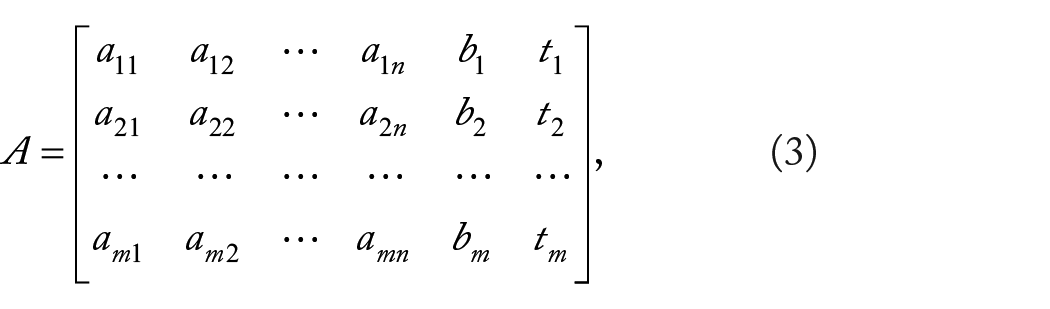
A = [\begin{matrix} a_{11} & a_{12} & \dots & a_{1 n} & b_{1} & t_{1} \\ a_{21} & a_{22} & \dots & a_{2 n} & b_{2} & t_{2} \\ \dots & \dots & \dots & \dots & \dots & \dots \\ a_{m 1} & a_{m 2} & \dots & a_{m n} & b_{m} & t_{m} \end{matrix}],

(3)

the set of preprocessed data, in which $A_{1}, \dots, A_{n}$ are the independent columns (air temperature, solar duration, wind speed, relative humidity, air pressure, and temperature), $B$ is the dependent one $(N O_{2}$ or $N O_{x}$ , depending on the problem we want to solve), ordered by the time of observation, and use a linear regression algorithm to extract a function of the type:

B (t) = c_{0} + \sum_{i = 1}^{n} c_{i} \cdot A_{i} (t) + ϵ .

(4)

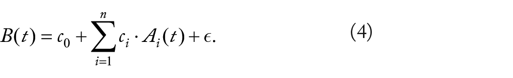
Solving this problem entails finding $n + 1$ optimal parameters (or coefficients) $c_{0}, c_{1}, \dots, c_{n}$ to fit the above equation, which does not take into account past values of any independent parameter, and the temporal component is used implicitly. Lagged (linear) regression consists of solving a more general equation, formulated as:

B (t) = c_{0} + \sum_{i = 1}^{n} \sum_{l = 0}^{p_{i}} c_{i, l} \cdot A_{i} (t - l) + ϵ .

(5)

In other words, we use the value of each independent variable $A_{i}$ not only at time $t$ but also at time $t - 1, t - 2, \dots, t - p_{i}$ , to explain $B$ at time $t$ ; each $A_{i} (t - l)$ is associated with a coefficient $c_{i, l}$ , which must be estimated, along with each maximum lag $p_{i}$ . There are available techniques, based on standard regression algorithms, that allow one to solve the inverse problem associated with equation (5); unfortunately, the resulting equation may result very difficult to interpret. Equation (5) is very similar to ARIMAX model, but without the autoregressive part.

Lagged regression can be performed with other, more complicate, model extraction methods that may not allow explicit representation, such as random forest or neural networks of any type. The underlying idea is the same: enhance the independent data by adding lagged versions of each variable $A - i$ up to a predetermined maximum $p_{i}$ .

Optimizing a lagged model

Both standard and lagged linear regression are classical, simple approaches to the problem of explaining the value of $B (t)$ (in our case, pollution concentrations), using current and past values of $A_{1}, \dots, A_{n}$ : having learned the best coefficients, the performances of the model are computed using standard measures. As per classical, standard data analysis procedures, the set $A$ may be used in $k$ -fold cross-validation mode to extract a linear model and test it at the same time, or separated into training and test subsets. In any case, solving equation (5) entails fixing the value $p_{i}$ for each independent variable; each past value of each independent variable may contribute in the same way to the model.

We work under the additional assumption that, for each $i$ , there is precisely 1 lag $l_{i}$ , such that $A_{i} (t - l_{i})$ influences the output more than any other lag; this may be reasonable in some applications, and less so in others: as we shall see, it fits perfectly our case. Under such an assumption, the model that we are assuming becomes:

B (t) = c_{0} + \sum_{i = 1}^{n} c_{i} \cdot A_{i} (t - l_{i}) + ϵ .

(6)

Our methodology can be described as follows: (1) we split the original data set $A$ into 2 sets that we call $A_{t r}$ and $A_{m o}$ , respecting the temporal ordering, (2) we optimize the values of $c_{0}, c_{1}, \dots, c_{n}$ , and $l_{1}, \dots, l_{n}$ on $A_{t r}$ , obtaining a linear model that fits $A_{t r}$ well, and (3) we use the obtained lags to transform $A_{m o}$ , so that a new model can be learned. Splitting into $A_{t r}$ and $A_{m o}$ is necessary to ensure that finding the optimal lags is computationally affordable: we search for the optimal lags in a small data set $(A_{t r})$ , and then we apply them to a bigger one $(A_{m o})$ , so that a model can be learned on the latter. The model that is learned on the transformed data can be of any type: linear (or, in general, functional), tree-based, or a neural network. The transformation gives us already some information on the problem itself, as it has optimized the delay after which a certain independent variable has effect; such a learned model, obtained on $A_{2}$ , can be tested using classical testing modes, such as training + test (which would entail further separating $A_{2}$ into 2 sets), or, as we shall do, $k$ -fold cross-validation. Observe that $A_{t r}$ cannot be considered a training set per se, but, instead, a pretraining set, used with the sole purpose of performing the optimization.

Having separated the optimization part from the training part, we can now arbitrarily complicate the model. For example, in some contexts, such as pollution concentration modeling, a super-linear explanation model may fit better than a linear one, yet preserving the possibility of an intuitive interpretation. From the mathematical point of view, the inverse problem that corresponds to searching for a super-linear model is a simple generalization of equation (6):

B (t) = c_{0} + \sum_{i = 1}^{n} c_{i} \cdot A_{i} {(t - l_{i})}^{e_{i}} + ϵ .

(7)

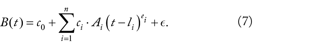
Thus, in the optimization part of our methodology, we can optimize coefficients $c_{i} s$ , lags $l_{i} s$ , and exponents $e_{i} s$ , for each predictor, and, then, apply this more elaborate transformation to the data. Once again, as a result of the optimization phase, we obtain new information; for example, we may learn that wind influences the amount of nitrogen oxide in the air at a certain moment with 2 hours of delay, and in a way proportional to the square of its strength. Even if we choose, in the second phase, to use a noninterpretable learning model (eg, random forest), we have more information on the underlying process than we would have had using the same learning model without transformation. Our purpose is to prove that such an optimization does increase the performances on the learned model in the second phase, independently from the specific learning model. A representation of this methodology can be found in Figure 2.

Figure 2.

A simple schematic of the proposed methodology.

Solving the optimization problem

Deciding the best lag and the best exponent for each variable is an optimization problem. Formally, given a multivariate time series $A_{1} (t), \dots, A_{n} (t), B (t)$ with $m$ distinct observations (such as our data on atmospheric pollution), let us define $P$ as the maximum lag of the problem (ie, we do not search solutions with lags greater than $P$ —observe that in equation (5), we have that $p_{i} = P$ for each $i)$ and $E$ as the maximum exponent of the problem (ie, we do not search solutions with exponents greater than $E$ —observe that in equation (7), we have that $e_{i} \leq E$ for each $i)$ . Let us fix a vector $\bar{x} = (x_{1}, \dots, x_{n})$ of decision variables with domain $[- 1, \dots, P] \subset ℕ$ , and let $M$ be the maximum of $\bar{x}$ (called maximum actual lag of $\bar{x})$ . The vector $\bar{x}$ entails a transformation of equation (3) into a new data set with $m - M$ observations, in which the feature (time series) $A_{i}$ is lagged (ie, delayed) of the amount ${\bar{x}}_{i}$ :

A (\bar{x}) = [\begin{matrix} a_{(M - {\bar{x}}_{1}) 1} & \dots & b_{M} & t_{M} \\ a_{((M + 1) - {\bar{x}}_{1}) 1} & \dots & b_{M + 1} & t_{M + 1} \\ \dots & \dots & \dots & \dots \\ a_{((m - M) - {\bar{x}}_{1}) 1} & \dots & b_{m - M} & t_{m - M} \end{matrix}] .

(8)

The transformation equation (8) works for every ${\bar{x}}_{i} \neq - 1$ . The case of ${\bar{x}}_{i} = - 1$ is interpreted as excluding the column $A_{i}$ from the problem (entailing an implicit FS method). Similarly, let $\bar{y} = (y_{1}, \dots, y_{n})$ , a second vector of decision variables with domain $[1, \dots, E]$ . For each variable $A_{i}$ , we interpret ${\bar{y}}_{i}$ as the exponent to which $A_{i}$ is raised in equation (7). So, in conjunction, the pair $\bar{x}, \bar{y}$ entails a transformation of equation (3) into a new data set with $m - M$ observations, in which the feature (time series) $A_{i}$ is lagged (ie, delayed) of the amount ${\bar{x}}_{i}$ , and raised to the power of ${\bar{y}}_{i}$ :

A (\bar{x}, \bar{y}) = [\begin{matrix} a_{(M - {\bar{x}}_{1}) 1}^{{\bar{y}}_{1}} & \dots & b_{M} & t_{M} \\ a_{((M + 1) - {\bar{x}}_{1}) 1}^{{\bar{y}}_{1}} & \dots & b_{M + 1} & t_{M + 1} \\ \dots & \dots & \dots & \dots \\ a_{((m - M) - {\bar{x}}_{1}) 1}^{\bar{y} - 1} & \dots & b_{m - M} & t_{m - M} \end{matrix}] .

(9)

A simple numeric example of such a transformation can be seen in Figure 3. In this example, we start off with 5 observations and 5 independent variables (the sixth column indicates the time of observation); the left-hand side (that contains the lags) of the decision variables vector contains 0 for the first and the fourth variable, 1 for the second variable, 3 for the fifth variable, and −1 for the third variable (which entails that this variable is not selected); the right-hand side (that contains the exponents) contains 1 (linear behavior) for every variable except the third one (which, by the way, is eliminated) and the fifth one, in which the exponent is 2 (quadratic behavior). The original data set, therefore, must contain 3 less observations because in this example, we are assuming that to explain the current value of $B$ , we need to look at the value of $A_{5}$ 3 units of time before. The values of the selected variables, at the selected times, are then elevated to the chosen exponent, instantiating equation (9).

Figure 3.

Example of transformation. The original data set (top) is transformed by the pair $\bar{x}, \bar{y}$ (middle) into a lagged data set (bottom), with 1 less feature. There are 3 less instances due to the maximum chosen lag.

Solving the optimization problem entails evaluating a vector $(\bar{x}, \bar{y})$ on $A_{t r}$ . As per our methodology, during the optimization phase, we use an efficient learner, such as linear regression, and any standard measure of the performances of the extracted model, such as the Pearson correlation test between the function values and the actual values of $B$ ; we denote such a generic function with $C O R R (\bar{x}, \bar{y})$ , that is, the correlation coefficient extracted by a linear regression algorithm ran on $A_{t r}$ after the transformation entailed by $\bar{x}, \bar{y}$ —correlation coefficient should be maximized. In a multiobjective context, however, we can also optimize the characteristics of both $\bar{x}$ and $\bar{y}$ . On one hand, we want to minimize the number of selected variables, using:

C A R D (\bar{x}) = \sum_{i = 1}^{n} {\begin{array}{l} 0 & i f {\bar{x}}_{i} \neq - 1 \\ 1 & o t h e r w i s e, \end{array}

(10)

and, on the other hand, we want to minimize the complexity of the extracted model, using:

M A X E X P (\bar{y}) = \max {{\bar{y}}_{i} | 1 \leq i \leq n} .

(11)

Thus, solving our optimization problem means instantiating equation (1) with:

{\begin{cases} \max C O R R (\bar{x}, \bar{y}) \\ \min C A R D (\bar{x}, \bar{y}), \\ \min M A X E X P (\bar{x}, \bar{y}) . \end{cases}

(12)

Clearly, other objective functions can be designed that may or may not improve the quality of the solutions.

Implementation

Multiobjective evolutionary algorithms are known to be particularly suitable to perform multiobjective optimization, as they search for multiple optimal solutions in parallel. In this experiment, we have chosen the well-known Nondominated Sorted Genetic Algorithm II,⁴⁹ which is available as open source from the suite jMetal.⁶² Nondominated Sorted Genetic Algorithm II is an elitist Pareto-based multiobjective evolutionary algorithm that employs a strategy with a binary tournament selection and a rank-crowding better function, where the rank of an individual in a population is the nondomination level of the individual in the whole population. As black box linear regression algorithm, during the optimization phase, we used the class LinearRegression from the open-source learning suite Weka,⁶³ run in 10-fold cross-validation mode, with standard parameters and no embedded FS. We have represented each individual solution (gene) as an array:

x_{1}, x_{2}, \dots, x_{n}, y_{1}, y_{2}, \dots, y_{n},

with values in $[- 1, \dots, L]$ for the $\bar{x}$ side and in $[1, \dots, E]$ for the $\bar{y}$ side.

The initial population has been generated randomly, in each execution, and the fitness functions reflect the objective functions of equation (12) in the obvious way; in particular, Weka implementation of any regression extraction algorithm returns, among other measures, the Pearson correlation coefficient of the extracted model. Mutation and crossover operations have been adapted to the form of the gene. To mutate an individual $I$ , we proceed as follows: (1) we randomly choose between the $x$ -part and $y$ -part; (2) we randomly choose the index to mutate; and (3) we randomly choose to mutate the corresponding value with an increment (plus 1), decrement (minus 1), or random substitution. Increments, decrements, and random substitutions are implemented in the interval $[- 1, \dots, L]$ in the $x$ -part, and in the interval $[0, \dots, E]$ in the $y$ -part. Similarly, crossover between 2 individuals $I, J$ is implemented as follows: (1) we randomly choose between the $x$ -part and $y$ -part; (2) we randomly choose 2 indexes in $I$ and 2 indexes in $J$ ; and (3) we perform the crossover on the selected indexes.

Experiment

According to the methodology described in Figure 2, we prepared the data sets $A_{t r}$ (7706 observations, 30% of the initial data) and $A_{m o}$ (17 981 observations, 70% of the initial data) for 2 problems, $N O_{2}$ and $N O_{x}$ , which we kept separated, for 2 different sets of experiments. We then run the optimization procedure with random initial population for 10 independent experiments, with seeds from 1 to 10. In the final population of each execution, we applied a simple decision-making strategy to choose 1 individual of the Pareto front, that is, the one with the best correlation coefficient, which is a natural choice. On each execution, we set the maximum lag at 6 hours $(P = 6)$ , and the maximum exponent at $(E = 3)$ . As it turns out, all selected solutions contain all initial variables, suggesting that all predictors do have an nontrivial role in the problem. The training results are shown in Table 2 for $N O_{2}$ , and in Table 3 for $N O_{x}$ . Both tables are structured in the same way. For each execution, we show the best correlation coefficient that we have obtained during training. Also, we show the lags, the exponents, and the coefficient for each variable, in the original order: temperature, solar radiation, wind, humidity, pressure, and traffic.

Table 2.

Training results for $N O_{2}$ .

exec.	lags	exp.	corr.	a	d	w	r	p	t
1	0,1,2,5,5,1	3,1,1,1,1,1	0.7272	0.0005	−12.2594	−5.5650	−0.3238	−0.0541	0.0086
2	5,0,2,5,1,1	2,1,1,1,2,1	0.7248	0.0155	−7.3854	−5.5652	−0.2308	−0.0000	0.0084
3	6,1,2,6,4,1	1,1,1,1,1,1	0.7246	0.2271	−7.4261	−5.5031	−0.3132	−0.0911	0.0089
4	5,6,2,5,0,1	3,3,1,3,3,1	0.7231	0.0006	6.5237	−5.5565	0.0000	0.0000	0.0077
5	0,0,2,6,0,1	3,1,1,1,1,1	0.7282	0.0005	−9.1026	−5.5726	−0.3215	−0.0957	0.0086
6	0,1,2,6,0,1	2,1,1,1,1,1	0.7286	0.0121	−10.5775	−5.5122	−0.3383	−0.0989	0.0089
7	1,1,2,6,1,1	3,1,1,1,1,1	0.7325	0.0005	−11.0236	−5.4998	−0.3202	−0.0833	0.0089
8	4,4,2,6,5,1	3,2,1,1,1,1	0.7253	0.0005	−0.4911	−5.5622	−0.2800	−0.0828	0.0081
9	6,1,2,6,0,1	3,2,1,1,1,1	0.7333	0.0006	−7.4740	−5.4309	−0.2524	−0.0847	0.0089
10	3,0,2,6,3,1	3,1,1,2,1,1	0.7295	0.0006	−7.9523	−5.5867	−0.0019	−0.0669	0.0086

We use exec. to indicate the execution number and exp. to denote the exponents. The variables are denoted as in Table 1.

Table 3.

Training results for $N O_{x}$ .

exec.	lags	exp.	corr.	a	d	w	r	p	t
1	2,5,2,0,6,1	1,2,1,1,1,1	0.6143	−2.3309	34.5527	−20.4060	1.3695	0.2496	0.0366
2	1,6,2,1,4,1	1,1,1,1,1,1	0.6194	−2.3091	40.2649	−19.9924	1.4599	0.1808	0.0371
3	1,6,2,1,6,1	1,1,1,2,3,1	0.6179	−2.4287	37.4455	−19.9698	0.0102	0.0000	0.0369
4	2,6,2,1,5,1	2,2,1,1,1,1	0.6135	−0.0529	46.6974	−19.4180	1.7456	0.3237	0.0369
5	0,5,2,1,3,1	1,1,1,1,1,1	0.6153	−2.1120	33.8346	−20.2968	1.4973	0.1574	0.0369
6	2,6,2,0,3,1	1,1,1,1,1,1	0.6156	−2.4368	34.3729	−20.4512	1.3020	0.1257	0.0368
7	1,6,2,0,0,0	1,1,1,1,1,1	0.6136	−2.4984	52.8382	−20.3610	1.3958	0.1049	0.0364
8	1,5,2,1,5,1	1,1,1,2,1,1	0.6151	−2.4271	32.8368	−20.3458	0.0100	0.1432	0.0365
9	0,6,2,1,6,1	1,1,1,1,1,1	0.6177	−2.0545	37.1161	−19.8380	1.5326	0.3469	0.0372
10	2,5,2,1,0,1	1,1,1,1,1,1	0.6156	−2.2025	39.7787	−20.1578	1.5233	0.1220	0.0364

We use exec. to indicate the execution number and exp. to denote the exponents. The variables are denoted as in Table 1.

As for the test phase, we have operated as follows: first, we have used the original test data set $(A_{m o})$ , with no transformations, to run 3 different regression algorithms, and, second, we have used the same algorithms over the data transformed with each of the 10 selected solutions, to measure the difference in performance, in 10-fold cross-validation mode. The algorithms that we have used are: (1) the classic linear regression (class LinearRegression in Weka—same parameters as in the optimization phase); (2) the random forest algorithm (class RandomForest in Weka—parameters: 100 trees, 100% size per bag, minimum 1 instance per leaf, $10^{- 3}$ maximum variance per leaf, unlimited depth per tree, no backfitting); (3) a multilayer perceptron (class MultilayerPerceptron in Weka—parameters: 0.3 learning rate, 0.2 momentum rate for backpropagation, 500 epochs, no validation set). Each execution of each learner has been run in 10-fold cross-validation mode, and, again, the column corr. denotes the result of the Pearson test of correlation, in average more than the 10 executions. We have also displayed the results of the standard residuals test: the mean absolute error, root mean squared error, the root absolute error, and the root squared error. The results of the test phase are shown in Tables 4 and 5.

Table 4.

Test results for $N O_{2}$ .

Algorithm	exec.	corr.	Mean a.e.	Root m.s.e.	Root a.e.	Root s.e.
Linear regression	orig	0.6395	12.9254	17.0113	74.4102	76.8771
	1	0.7277	11.6018	15.1785	66.7858	68.5889
	2	0.7230	11.6794	15.2869	67.2320	69.0789
	3	0.7343	11.4391	15.0208	65.8503	67.8766
	4	0.7143	11.8412	15.4869	68.1693	69.9880
	5	0.7288	11.5700	15.1522	66.6039	68.4707
	6	0.7330	11.4887	15.0535	66.1362	68.0245
	7	0.7314	11.5169	15.0909	66.2948	68.1899
	8	0.7210	11.7094	15.3326	67.4067	69.2859
	9	0.7291	11.5687	15.1442	66.5966	68.4342
	10	0.7249	11.6236	15.2423	66.9125	68.8779
Random forest	orig	0.7538	10.8476	14.5395	62.4486	65.7067
	1	0.8017	9.9405	13.2286	57.2222	59.7779
	2	0.8045	9.9706	13.1447	57.3953	59.3985
	3	0.8053	9.9360	13.1207	57.1974	59.2904
	4	0.7939	10.1857	13.4576	58.6348	60.8129
	5	0.8082	9.8223	13.0336	56.5431	58.8969
	6	0.8009	10.0009	13.2611	57.5731	59.9246
	7	0.8025	9.9220	13.2069	57.1181	59.6831
	8	0.7976	10.1043	13.3791	58.1656	60.4569
	9	0.8042	9.9336	13.1500	57.1809	59.4230
	10	0.8082	9.8646	13.0500	56.7855	58.9700
Multilayer perceptron	orig	0.6115	13.6077	18.1439	78.3378	81.9954
	1	0.6381	13.4738	17.4629	77.5618	78.9117
	2	0.6428	13.3944	17.3457	77.1046	78.3820
	3	0.6678	12.9831	16.8019	74.7383	75.9253
	4	0.6365	13.5315	17.4957	77.8953	79.0603
	5	0.6677	13.0059	16.7383	74.8696	75.6378
	6	0.6630	13.1540	16.9416	75.7225	76.5567
	7	0.6610	13.1991	17.0009	75.9824	76.8260
	8	0.6310	13.7787	17.7409	79.3165	80.1723
	9	0.6581	13.2655	17.0754	76.3666	77.1592
	10	0.6666	12.9946	16.7427	74.8048	75.6580

We use exec. to indicate the execution number, and corr. (mean a.e., root m.s.e., root a.e., and root s.e.) to denote the correlation index (the mean absolute error, the root mean squared error, the root absolute error, and the root standard error, respectively).

Table 5.

Test results for $N O_{x}$ .

Algorithm	exec.	corr.	Mean a.e.	Root m.s.e.	Root a.e.	Root s.e.
Linear regression	orig	0.6381	51.3114	76.1511	70.6137	76.9965
	1	0.6743	49.4777	73.0408	68.0773	73.8382
	2	0.6803	49.1245	72.4960	67.5914	73.2874
	3	0.6782	49.3159	72.6908	67.8548	73.4843
	4	0.6748	49.3625	72.9961	67.9188	73.7929
	5	0.6732	49.4706	73.1357	68.0714	73.9390
	6	0.6769	49.3169	72.8089	67.8561	73.6037
	7	0.6842	48.8029	72.1356	67.1488	72.9230
	8	0.6747	49.4927	73.0056	68.1018	73.8075
	9	0.6761	49.3532	72.8781	67.9061	73.6736
	10	0.6766	49.2547	72.8330	67.7743	73.6330
Random forest	orig	0.7343	43.3031	67.1449	59.5929	67.8904
	1	0.7660	41.3382	63.6004	56.8780	64.2947
	2	0.7721	41.0314	62.8687	56.4560	63.5550
	3	0.7715	41.0264	62.9431	56.4490	63.6302
	4	0.7629	41.7022	63.9675	57.3789	64.6658
	5	0.7643	41.4665	63.7992	57.0577	64.5000
	6	0.7665	41.3807	63.6612	56.9365	64.3561
	7	0.7741	40.4066	62.6275	55.5962	63.3112
	8	0.7685	41.1358	63.2970	56.6027	63.9922
	9	0.7717	41.0702	62.9229	56.5093	63.6097
	10	0.7644	41.3297	63.7875	56.8694	64.4882
Multilayer perceptron	orig	0.6162	54.8119	78.5257	75.4311	79.3974
	1	0.6396	53.2879	77.5143	73.3199	78.3605
	2	0.6312	54.8395	78.4361	75.4548	79.2923
	3	0.6187	55.2503	79.0517	76.0200	79.9146
	4	0.6309	54.6739	78.1931	75.2270	79.0467
	5	0.6494	50.9036	76.1172	70.0431	76.9532
	6	0.6364	53.7965	77.8218	74.0197	78.6713
	7	0.6554	51.5772	75.4753	70.9660	76.2990
	8	0.6577	50.3422	75.3777	69.2706	76.2057
	9	0.6307	54.6624	78.3721	75.2111	79.2276
	10	0.6523	50.7901	75.8542	69.8870	76.6874

Discussion

In view of the results that have been obtained, 2 important elements emerge: first, how lags and nonlinear contributions are explained in the physical process, and, second, how the transformations improve the synthesis of regression models. As much as the first point is concerned, it is important to understand that different executions may give rise to different results and yet similar performances. On one side, some lags are consistent in all executions, which indicates that the temporal component of their contribution is stable and clear. On the other side, some lags and some individual coefficients do show certain variability: we believe that in such cases, more experiments are necessary to fully understand the underlying mechanisms. All notwithstanding, it is clear how convolution vectors have a clear positive effect on the cross-validated performances across the entire spectrum of algorithms for regression that we have tried. The following considerations can be done.

Traffic influences the amount of pollutant concentrations in a positive way, and with 1 hour of delay; this delay can be explained by the fact that the effect of exhaust gases needs some time to accumulate (observe, also, that we are limited by the granularity of observations: if sensors had collected data with granularity, say, 1 minute, we may have seen shorter delays for this variable).

Higher air temperatures are associated with a decrease in $N O_{2}$ and $N O_{x}$ concentrations, which is caused by 3 processes: (1) at higher air intake temperatures, less $N O_{2}$ is produced in the process of fuel combustion in the engine; (2) higher air temperatures usually imply more favorable atmospheric conditions, which encourage residents to use alternative means of transportation which reduces traffic volume⁶⁴; and (3) $N O_{2}$ is dynamically transformed into $N O$ (and back) at a higher rate with higher temperatures.

Wind always affects concentration in a negative way, with a constant (across different executions) delay of 2 hours. This is probably due to the distance between the intersection and the meteorological station; the average wind speed of 3 m s⁻¹ and the roughness of terrain explain the amount of the delay.

Higher humidity may cause a decrease in $N O_{2}$ concentration in exhaust gases^65,66 ; we have found that such an effect takes place with 5 to 6 hours of delay.

High solar duration and high temperature favor the transformation of nitrogen oxides into secondary pollutants, which include ozone, and this implies a decrease in $N O_{x}$ concentration; even more important is sunlight, which acts as a catalyst, which explains the negative coefficient and the delay for sunlight duration.

Of how the transformation influences the synthesis of good regression models, we can observe what follows. First, not all models show the same improvement, but all models show some improvement. In the case of $N O_{2}$ , the models extracted with linear regression showed a maximum improvement of 0.948 in correlation, those with random forest of 0.544, and those with multilayer perceptron of 0.563, and in the case of $N O_{x}$ , the improvements have been of 0.461, 0.398, and 0.415, respectively. Also, observe that there was an improvement in every independent execution, indicating that the results are stable. The fact that linear regression presented the most evident improvement is expected, given that used the same algorithm for optimization. Second, the improvement in predicting the $N O_{2}$ concentration is greater than the one in predicting $N O_{x}$ , probably due to the fact that the latter is a more complex problem. Third, linear regression and random forest show greater improvements than multilayer perceptron; the latter, however, shows low results even with nontransformed data, possibly suggesting that the underlying problem is not highly nonlinear enough to require, and justify, a neural network–based approach.

Comparing our results from the statistical point of view with those that can be obtained by other, well-known, methods is quite difficult. Take $N O_{2}$ prediction models, for example. Running simple, atemporal, linear regression on the same data yields a correlation coefficient that, in average, is 0.678 in test (single execution). The extracted model is:

\begin{array}{l} N O_{2} = - 0.2345 a - 12.8184 d - 5.4104 w - 0.2244 h \\ = - 0.1771 p + 0.0083 t + 245.3536 . \end{array}

(13)

While the coefficients are not too dissimilar from those obtained with the transformations, the reduced correlation shows that delays must be taken into account. Running full lagged models, on the other hand, leads, in some cases, to higher correlations. Unfortunately, the resulting models are impossible to be interpreted from the environmental point of view. Just for example, the simplest full lagged model that we tried, with 6 hours of maximum delay for each variable (ie, with 36 independent variables), already leads to positive and negative coefficients of the same independent variables at different delays: the variable temperature, for instance, presents positive coefficients for lag 0, 4, and 6, and negative ones in all the other lags. A possible explanation of this phenomenon is that by artificially increasing the number of independent variables (such as it is done when several lagged variables are added for each parameter), one allows regression algorithms to find artificially good solutions by using many hyperplanes; in other words, the solution tends to overfit even in presence of several thousands of data instances. Overfitting models are less reliable explanatory models because they tend not to be associated with physical explanations.

Conclusions

In this article, we have approached the problem of devising an explanation model for $N O_{2}$ and $N O_{x}$ concentrations observed via a monitoring station in the city of Wrocław (Poland). First, we revised the current literature on prediction, forecasting, and explanation models for temporal series. Then, we formulated the problem of finding an explanation model for air pollution as a lagged regression problem, and designed an optimization problem whose solutions are precisely the optimal lags for regression. Finally, we proposed realistic and physically explicable lagged regression models for both $N O_{2}$ and $N O_{x}$ concentrations based on available data from 2015 to 2017, induced with our method. We obtained significative improvements in the coefficient of determination over nonlagged regression models, while retaining (in fact, easing) the interpretability of the resulting equations. Our technology is immediately applicable to the same problems with different data, as well as to similar problems in which the temporal component plays an essential role. Time series explaining is less common in the technical literature than time series forecasting. Yet, forecasting is not focused on interpretability, often resulting in (sometimes, statistically reliable) black box models which, however, offer no explanation of the underlying phenomena. For future work, we plan to improve our design by allowing our optimization schema to consider reasonable temporal combinations of lagged variables, yet retaining the superior interpretability degree of lagged models over statistical forecasting.

Footnotes

Funding:

The author(s) disclosed receipt of the following financial support for the research, authorship, and/or publication of this article: The authors acknowledge the partial support from the following projects: Artificial Intelligence for Improving the Exploitation of Water and Food Resources, founded by the University of Ferrara under the FIR program, and New Mathematical and Computer Science Methods for Water and Food Resources Exploitation Optimization, founded by the Emilia-Romagna region, under THE POR-FSE PROGRAM.

Declaration of conflicting interests:

The author(s) declared no potential conflicts of interest with respect to the research, authorship, and/or publication of this article.

Author Contributions

GS: experiment’s conception and design, results’ technical interpretation, and text writing. EL-S: implementation, test, and text writing. JK: data providing, results’ physical interpretation.

ORCID iD

Guido Sciavicco

References

Kowalska

Skrzypek

Kowalski

, et al. The relationship between daily concentration of fine particulate matter in ambient air and exacerbation of respiratory diseases in Silesian agglomeration, Poland. Int J Environ Res Public Health. 2019;16:1131.

Holnicki

Tainio

Kałuszko

, et al. Burden of mortality and disease attributable to multiple air pollutants in Warsaw, Poland. Int J Environ Res Public Health. 2017;14:1359.

Schwartz

Lung function and chronic exposure to air pollution: a cross-sectional analysis of NHANES II. Environ Res. 1989;50:309-321.

Cesaroni

Badaloni

Gariazzo

, et al. Long-term exposure to urban air pollution and mortality in a cohort of more than a million adults in Rome. Environ Health Perspect. 2013;121:324-331.

Peng

Dominici

Louis

TA.

Model choice in time series studies of air pollution and mortality. J Royal Stat Soc Series A Stat Soc. 2006;169:179-203.

Schwartz

Air pollution and blood markers of cardiovascular risk. Environ Health Perspect. 2001;109:405-409.

Mar

Norris

Koenig

Larson

TV.

Associations between air pollution and mortality in Phoenix, 1995-1997. Environ Health Perspect. 2000;108:347-353.

Vanos

Cakmak

Kalkstein

Yagouti

Association of weather and air pollution interactions on daily mortality in 12 Canadian cities. Air Qual Atmos Health. 2015;8:307-320.

Knibbs

de Waterman

AMC

Toelle

, et al. The Australian child health and air pollution study: a national population-based cross-sectional study of long-term exposure to outdoor air pollution, asthma, and lung function. Environment International. 2018;120:394-403.

10.

Cifuentes

Vega

Köpfer

Lave

LB.

Effect of the fine fraction of particulate matter versus the coarse mass and other pollutants on daily mortality in Santiago, Chile. J Air Waste Manag Assoc. 2000;50:1287-1298.

11.

Kryza

Szymanowski

Dore

, et al. Application of a land use regression model for calculation of the spatial pattern of annual

N O_{x}

air concentrations at national scale: a case study for Poland. Proc Environ Sci. 2011;7:98-103.

12.

Aguilera

Foraster

Basagaña

, et al. Application of land use regression modelling to assess the spatial distribution of road traffic noise in three European cities. J Expo Sci Environ Epidemiol. 2015;25:97-105.

13.

Box

Jenkins

Reinsel

, et al. Time Series Analysis: Forecasting and Control. London, UK: Wiley; 2016.

14.

Hall

Time series analysis and forecasting with WEKA, 2014. https://wiki.pentaho.com/display/DATAMINING/Time+Series+Analysis+and+Forecasting+with+Weka.

15.

Jollois

Poggi

Portier

Three non-linear statistical methods for analyzing PM10 pollution in Rouen area. Case Stud Bus Indus Govern Stat. 2009;3:1-17.

16.

Cobourn

Bai

Development of nonlinear empirical models to forecast daily

P M_{2.5}

and ozone levels in three large Chinese cities. Atmosp Environ. 2016;147:209-223.

17.

Singh

Gupta

Kumar

, et al. Linear and nonlinear modeling approaches for urban air quality prediction. Sci Total Environ. 2012;426:244-255.

18.

Cobourn

WG.

An enhanced

P M_{2.5}

air quality forecast model based on nonlinear regression and back-trajectory concentrations. Atmosph Environ. 2010;44:3015-3023.

19.

Shi

Harrison

RM.

Regression modelling of hourly

N O_{x}

and

N O_{2}

concentrations in urban air in London. Atmosp Environ. 1997;31:4081-4094.

20.

Maciag

Kasabov

Kryszkiewicz

, et al. Air pollution prediction with clustering-based ensemble of evolving spiking neural networks and a case study for London area. Environ Model Software. 2019;118:262-280.

21.

Kamińska

JA.

The use of random forests in modelling short-term air pollution effects based on traffic and meteorological conditions: a case study in Wrocław. J Environ Manage. 2018;217:164-174.

22.

Balashov

Thompson

Young

GS.

Probabilistic forecasting of surface ozone with a novel statistical approach. J Appl Meteorol Climatol. 2017;56:297-316.

23.

Aznarte

JL.

Probabilistic forecasting for extreme

N O_{2}

pollution episodes. Environ Pollut. 2017;229:321-328.

24.

Cabaneros

Calautit

Hughes

BR.

A review of artificial neural network models for ambient air pollution prediction. Environ Model Software. 2019;119:285-304.

25.

Kamińska

JA.

A random forest partition model for predicting

N O_{2}

concentrations from traffic flow and meteorological conditions. Sci Total Environ. 2019;651:475-483.

26.

Sayegh

Tate

Ropkins

Understanding how roadside concentrations of

N O_{x}

are influenced by the background levels, traffic density, and meteorological conditions using boosted regression trees. Atmosp Environ. 2016;127:163-175.

27.

Singh

Gupta

Rai

Identifying pollution sources and predicting urban air quality using ensemble learning methods. Atmosp Environ. 2013;80:426-437.

28.

Shang

Deng

, et al. A novel model for hourly

P M_{2.5}

concentration prediction based on CART and EELM. Sci Total Environ. 2019;651:3043-3052.

29.

Zhai

Chen

Development of a stacked ensemble model for forecasting and analyzing daily average

P M_{2.5}

concentrations in Beijing, China. Sci Total Environ. 2018;635:644-658.

30.

Kamińska

JA.

Probabilistic forecasting of nitrogen dioxide concentrations at an urban road intersection. Sustainability. 2018;10:1-16.

31.

Holt

Forecasting seasonals and trends by exponentially weighted moving averages. Int J Forecast. 2004;20:5-10.

32.

Winters

Forecasting sales by exponentially weighted moving averages. Manage Sci. 1960;3:324-342.

33.

Poulos

Kvanli

Pavur

A comparison of the accuracy of the box-Jenkins method with that of automated forecasting methods. Int J Forecast. 1987;3:261-267.

34.

Hochreiter

Schmidhuber

Long short-term memory. Neural Comput. 1997;9:1735-1780.

35.

Russo

Lind

Raischel

, et al. Neural network forecast of daily pollution concentration using optimal meteorological data at synoptic and local scales. Atmosp Pollut Res. 2015;6:540-549.

36.

Vlachogiannis

Sfetsos

. Time series forecasting of hourly pm10 values: model intercomparison and the development of localized linear approaches:85-94. https://www.witpress.com/Secure/elibrary/papers/AIR06/AIR06009FU1.pdf.

37.

Brunello

Kaminska

Marzano

, et al. Assessing the role of temporal information in modelling short-term air pollution effects based on traffic and meteorological conditions: a case study in Wrocław. In: Proceedings of the Workshop New Trends in Databases and Information Systems, Communications in Computer and Information Science, Vol. 1064. Berlin: Springer; 2019:463-474.

38.

Analitis

Katsouyanni

Dimakopoulou

, et al. Short-term effects of ambient particles on cardiovascular and respiratory mortality. Epidemiology. 2006;17:230-233.

39.

Liu

Zhang

, et al. The short-term effect of ambient ozone on mortality is modified by temperature in Guangzhou, China. Atmosp Environ. 2013;76:59-67.

40.

Parodi

Vercelli

Garrone

Fontana

Izzotti

Ozone air pollution and daily mortality in Genoa, Italy between 1993 and 1996. Public Health. 2005;119:844-850.

41.

Catalano

Galatioto

Bell

, et al. Improving the prediction of air pollution peak episodes generated by urban transport networks. Environ Sci Policy. 2016;60:69-83.

42.

Wang

Mao

Eriksson

A three-dimensional Dijkstra’s algorithm for multi-objective ship voyage optimization. Ocean Eng. 2019;186.

43.

Kollat

Reed

PM.

Comparing state-of-the-art evolutionary multi-objective algorithms for long-term groundwater monitoring design. Adv Water Res. 2006;29:792-807.

44.

Madsen

Automatic calibration of a conceptual rainfall-runoff model using multiple objectives. J Hydrol. 2000;235:276-288.

45.

Pal

Galelli

A numerical framework for the multi-objective optimal design of check dam systems in erosion-prone areas. Environ Model Software. 2019;119:21-31.

46.

Qiu

Shen

Leng

, et al. Impacts of climate change on watershed systems and potential adaptation through BMPs in a drinking water source area. J Hydrol. 2019;573:123-135.

47.

Guyon

Elisseeff

. An introduction to variable and feature selection. J Mach Learn Res. 2003:1157-1182.

48.

Collette

Siarry

Multiobjective Optimization: Principles and Case Studies. Berlin; Heidelberg: Springer; 2004.

49.

Deb

Multi-Objective Optimization Using Evolutionary Algorithms. London, UK: Wiley; 2001.

50.

Jiménez

Sánchez

García

, et al. Multi-objective evolutionary feature selection for online sales forecasting. Neurocomput. 2017;234:75-92.

51.

Emmanouilidis

Hunter

Macintyre

, et al. A multi-objective genetic algorithm approach to feature selection in neural and fuzzy modeling. Evolut Optim. 2001;3:1-26.

52.

Mukhopadhyay

Maulik

Bandyopadhyay

, et al. A survey of multiobjective evolutionary algorithms for data mining: part I. IEEE Trans Evolut Comput. 2014;18:4-19.

53.

Siedlecki

Sklansky

. A note on genetic algorithms for large-scale feature selection. In: Chen

(ed.) Handbook of Pattern Recognition and Computer Vision. Singapore: World Scientific; 1993:88-107.

54.

Ishibuchi

Nakashima

. Multi-objective pattern and feature selection by a genetic algorithm. In: Proceedings of the Genetic and Evolutionary Computation Conference; 2000:1069-1076. http://www.cs.osakafu-u.ac.jp/ci/Papers/pdf_file/multiobjective/GECCO_2000_PF_Selection.pdf.

55.

Liu

Iba

. Selecting informative genes using a multiobjective evolutionary algorithm. In: Proceedings of the 2002 Congress on Evolutionary Computation, Vol. 1. New York, NY: IEEE; 2002:297-302.

56.

Pappa

Freitas

Kaestner

. Attribute selection with a multi-objective genetic algorithm. In: Proceedings of the 16th Brazilian Symposium on Artificial Intelligence. New York, NY: IEEE; 2004:280-290.

57.

Shi

Suganthan

Deb

. Multiclass protein fold recognition using multiobjective evolutionary algorithms. In: Proceedings of the 2004 Symposium on Computational Intelligence in Bioinformatics and Computational Biology. New York, NY: IEEE; 2004:61-66.

58.

García-Nieto

Alba

Jourdan

, et al. Sensitivity and specificity based multiobjective approach for feature selection: application to cancer diagnosis. Inform Process Lett. 2009;109:887-896.

59.

Jiménez

Jódar

Martín

, et al. Unsupervised feature selection for interpretable classification in behavioral assessment of children. Expert Syst. 2017;34:1-15.

60.

Jiménez

Martínez

Marzano

, et al. Multiobjective evolutionary feature selection for fuzzy classification. IEEE Trans Fuzzy Syst. 2019;27:1085-1099.

61.

Sarigiannis

Saisana

Multi-objective optimization of air quality monitoring. Environ Monit Assess. 2008;136:87-99.

62.

Durillo

Nebro

Jmetal: a Java framework for multi-objective optimization. Adv Eng Software. 2011;42:760-771.

63.

Witten

Frank

Hall

Data Mining: Practical Machine Learning Tools and Techniques, 3rd edn. USA: Morgan Kaufmann, Elsevier; 2011.

64.

Chalfen

Kamińska

Analiza wykorzystania roweru miejskiego we wrocławiu (in Polish). Autobusy Technika, Eksploatacja, Systemy Transportowe. 2016;17:543-545.

65.

Toback

Hearne

Kuritz

, et al. The effect of ambient temperature and humidity on measured idling emissions from diesel school buses. SAE Trans. 2004;113:530-538.

66.

Krause

Merrion

Green

GL.

Effect of inlet air humidity and temperature on diesel exhaust emissions. SAE Trans. 1973;82:831-837.

Temporal Aspects in Air Quality Modeling—A Case Study in Wrocław

Abstract

Keywords

Introduction

Background

Mathematical models for air quality prediction and explanation

Time series and lagged models

Feature selection

Multiobjective optimization

Data

Method

Lagged regression

Optimizing a lagged model

Solving the optimization problem

Implementation

Experiment

Discussion

Conclusions

Footnotes

Funding:

Declaration of conflicting interests:

Author Contributions

ORCID iD

References