
Abstract
It is necessary to accurately capture the growth trajectory of fluorescence where the best fit, precision, and relative efficiency are essential. Having this in mind, a new family of growth functions called TWW (Tabatabai, Wilus, Wallace) was introduced. This model is capable of accurately analyzing quantitative polymerase chain reaction (qPCR). This new family provides a reproducible quantitation of gene copies and is less labor-intensive than current quantitative methods. A new cycle threshold based on TWW that does not need the assumption of equal reaction efficiency was introduced. The performance of TWW was compared with 3 classical models (Gompertz, logistic, and Richard) using qPCR data. TWW models the relationship between the cycle number and fluorescence intensity, outperforming some state-of-the-art models in performance measures. The 3-parameter TWW model had the best model fit in 68.57% of all cases, followed by the Richard model (28.57%) and the logistic (2.86%). Gompertz had the worst fit in 88.57% of all cases. It had the best precision in 85.71% of all cases followed by Richard (14.29%). For all cases, Gompertz had the worst precision. TWW had the best relative efficiency in 54.29% of all cases, while the logistic model was best in 17.14% of all cases. Richard and Gompertz tied for the best relative efficiency in 14.29% of all cases. The results indicate that TWW is a good competitor when considering model fit, precision, and efficiency. The 3-parameter TWW model has fewer parameters when compared to the Richard model in analyzing qPCR data, which makes it less challenging to reach convergence.
Keywords
Introduction
Mathematical modeling of growth dynamics using observational or experimental data has been a major tool in computational biology for many years. The purpose of this article is to introduce a new mathematical growth model capable of accurately modeling biological, medical, socioeconomic, and engineering data. These models can be applied to tumor growth (either measured as the number of cells or as the volume of a multicellular sphere), human and animal growth, plant growth, and both adult and embryonic stem cell proliferation.1-3 In 1798, the exponential growth model was introduced by Thomas Robert Malthus manifesting his concept of population growth. 4 In 1838, the logistic growth model was introduced by Pierre Francois Verhulst by modifying the exponential growth and imposing a constraint based on the limited availability of resources. 4 In 1825, Benjamin Gompertz proposed the Gompertz growth model which has been frequently applied to biomedical data. 5 Around 1957, Ludwig von Bertalanffy introduced a model for animal growth. In his model, he explains the animal growth while taking into consideration the growth of the animal as the result of anabolism and catabolism of body materials. 6 The Richard growth model was introduced in 1959 as a generalization of the logistic growth model. 7 In 1981, Jon Schnute introduced his growth model which can represent logistic, Gompertz, Bertalanffy, and Richard models as its special cases.7,8 Tumor spheroids were used to characterize the growth dynamics and response to different treatments. 9
Mathematical modeling is a key process to describe the behavior of biological networks. The purpose is to build a model that predicts the state of a biological phenomenon as a function of one or more predictor variables. According to Ghisletta et al, 10 rather than solely using linear or quadratic growth models, one should consider appropriate nonlinear alternatives.
Modeling growth dynamics of biological and clinical data, which include both experimental and control groups, would have provided invaluable information regarding disease progression and regression. It will also shed light on the study of biological systems from molecules to organism and the population level.11-13
These quantitative models, alongside stem cell research, may possibly lead to novel treatments. 14 The sigmoidal growth models such as logistic, Gompertz, Bertalanffy, and Richard have been extensively used to model self-limited population growth in fields such as biology, economics, sociology, fishery, forestry, animal science, agriculture, and medical sciences.15-20 Initially, the rate of growth increases at the early stage and then gradually decreases to zero when the biomass of the organism reaches its carrying capacity. The logistic growth model has a symmetric curve with a fixed inflection point, which is at half of its carrying capacity, while the Gompertz growth rate is asymmetric. On the contrary, the Richard growth has flexible point of inflection.5,7,21 The Richard equation generalizes the logistic and Gompertz equations.22,23 The Hill model is widely used in pharmacodynamics, pharmacokinetics, and pharmacology for analyzing dose-response data. 24 The pharmacologist normally compares samples of treated and untreated cells at different levels of drug concentrations. Special cases of these growth functions can also serve as an activation function in machine learning. 25
In 2005, Tabatabai et al 1 introduced the hyperbolastic models of types I, II, and III, in the context of developing models with more versatility in representing actual growth rates from experimental data. The models have proven to have high precision in the representation of biological growth data, with close approximations to experimental results. These models have been particularly accurate in representation of cellular growth, such as growth of tumor cells 26 or growth of stem cells.27-29
In this article, a new growth model named TWW (Tabatabai, Wilus, Wallace) is introduced. This new model is used to analyze the well-known method of multiplying genetic sequences, polymerase chain reaction (PCR), which may be operated in a real-time calibrated mode known as quantitative PCR (qPCR). Quantitative polymerase chain reaction is a type of PCR that allows quantification of specific DNA and RNA targets. The qPCR method measures the intensity of stimulated emission released by the fluorescence probe at each end of a thermal heat cycle. A qPCR cycle curve has an exponential phase and a plateau phase. Quantitative polymerase chain reaction can amplify, detect, and quantify nucleic acids. The quantification can be absolute or relative.30-32 Applications of qPCR include, but not limited to, the measurement and analysis of gene expression data, identification of the genetic building that is present within a set of genotyped entities, pathogen detection, the genomic link between disease and single-nucleotide polymorphism (SNP) markers and forensic sciences.33,34
The cycle threshold (Ct) is a PCR cycle which represents the number of cycles required for the fluorescent signal to cross the threshold. The Ct values are inversely related to the volume of nucleic acid in the sample. 35 The qPCR is grounded on the fact that at each cycle, the number of PCR products doubles. The Ct value is typically defined as 5 to 10 standard deviations (SDs) in the noise floor and may lie in the range of 20 to 30 PCR cycles. Ct values are related to the number of nucleic acid molecules in the sample as reported by the fluorescence signal.
A higher Ct value may indicate a lower initial messenger ribonucleic acid (mRNA) molecular count. A gene which is highly expressed would typically have a lower Ct value needed. For example, a higher DNA/RNA molecular count in the initial sample would support a lower Ct value. 36
Guescini et al proposed a new method called
Method
The models commonly used in literature to analyze qPCR data are Richard, logistic, and Gompertz. For comparative purposes, a 5-parameter Richard model defined as

was used throughout this study. The fluorescence intensity at cycle number

and the 3-parameter Gompertz model with the following equation

were used throughout this article.
TWW growth model
The 3-parameter TWW growth model

is equal to

Alternatively, the growth rate equation (1) can be written as

where the relative growth rate
When the parameter
The point of inflection for the graph of equation (2) is

with
The slope of the tangent line to the graph of

which can be approximated as

If one desires to calculate the point

An alternative but equivalent form of the 3-parameter growth function

and the growth rate

Equation (3) is equivalent to equation (2) when
A third form of a 3-parameter TWW growth function

Equation (5) is also equivalent to equation (2) when
The corresponding growth rate function using equation (5) is

In the event that a 3-parameter TWW did not fit the data adequately well, we recommend that one should try the 4-parameter TWW model of the form

where
A 5-parameter TWW model has the form

where
In some cases of fluorescence of bacterial cultures or microbial data, it may be more appropriate to use a 4- or 5-parameter TWW model if the 3-parameter does not fit the data adequately enough. 37
Multivariable TWW growth model
If the function F depends on a set of independent variables
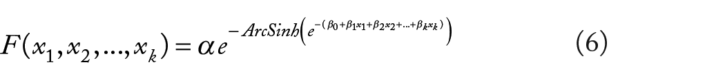
where
For
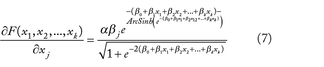
Partial elasticity
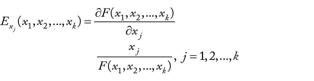
The partial elasticity of growth with respect to independent variable
For discrete variables, the partial elasticity is calculated using

For TWW growth model using equation (7), the partial elasticity is given by

This partial elasticity approximates the percentage change in growth divided by percentage change in the independent variable

where
Figure 1 illustrates the growth functions as well as their respective growth rate functions for different combinations of parameters. The graphs show the flexibility of the 3-parameter TWW growth models with respect to change in parameter values.

TWW growth and growth rate functions using different parameter values.
Figure 2 shows 3D graphs of growth and growth rate as a function of independent variables and a single parameter while holding the remaining parameters at a fixed level.

3D graphs of growth and growth rate functions under different conditions.
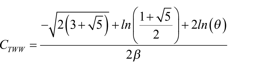
Evaluation of TWW cycle threshold
For the 3-parameter TWW model, the first step in calculating
The next step is to calculate the slope of the tangent line to the graph of the 3-parameter function

and can be approximated as

As shown in Figure 3, the cycle number
which can be approximated as

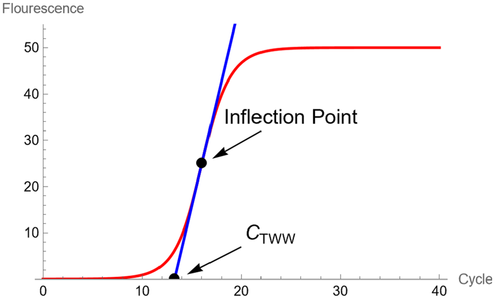
Shows the fluorescence intensity and the tangent line crossing the horizontal axis, creating the
If one uses a 4-parameter TWW function, then the point of inflection

and

The slope of the tangent line to the graph of

The

with an approximate value of

The 5-parameter TWW model has its point of inflection at

and

The slope of the tangent line to the graph of the 5-parameter

and the

Measures of fit, precision, and relative efficiency
Using PCR data of Guescini et al 35 and for each combination of input molecular number and amplification mix, the average fluorescence sample over the 12 runs was calculated. Then, the 3-parameter TWW growth function, the 3-parameter Gompertz, the 3-parameter logistic, and the 5-parameter Richard functions were used to estimate the fluorescence intensity as a function of cycle number for all 4 models using the PROC NLIN function in SAS software version 9.4 with the Gauss-Newton method. To assess the fit performances of the 4 models, qPCR data were used to calculate Akaike information criterion (AIC) and Bayesian information criterion (BIC) which have been defined as

and

where n is the sample size,
A model with a lower AIC and BIC provides a reasonable fit and would be selected. For each combination of input molecular number and amplification mix, AIC and BIC for all 4 models were calculated.
Additional performance measures considered are precision and relative efficiency metrics. For each combination of input molecular number and amplification mix, the precision (Pre) was calculated using the following equation:

where

where
Results
Table 1 provides the AIC and BIC values for all 4 models. For 68.57% of combination of input molecular number and amplification mix cases, the 3-parameter TWW model had the least values for AIC and BIC, indicating the best model fit among all models considered in this study. The Richard model was the best fit only in 28.57% of all cases, and the logistic was best in 2.86% of all cases. The Gompertz was the worst fit for 88.57% of all cases.
Values of AIC and BIC for TWW, Gompertz, logistic, and Richard models.

Table 2 shows the computed values for precision and relative efficiencies. TWW had the best precision 85.71% of all cases while the Richard model had the highest precision with only 14.29%. For all cases, Gompertz had the worst precision when compared with other models. TWW had the best relative efficiency 54.29% of all cases, while logistic relative efficiency was the best in only 17.14%. Richard and Gompertz tied for best relative efficiency each with approximately 14.29% of all cases.
Precision and relative efficiency for TWW, Gompertz, logistic, and Richard models.

Table 3 shows the values of
Values of


TWW model fit to the PCR data at different amplification mix for all 7 input molecular numbers.
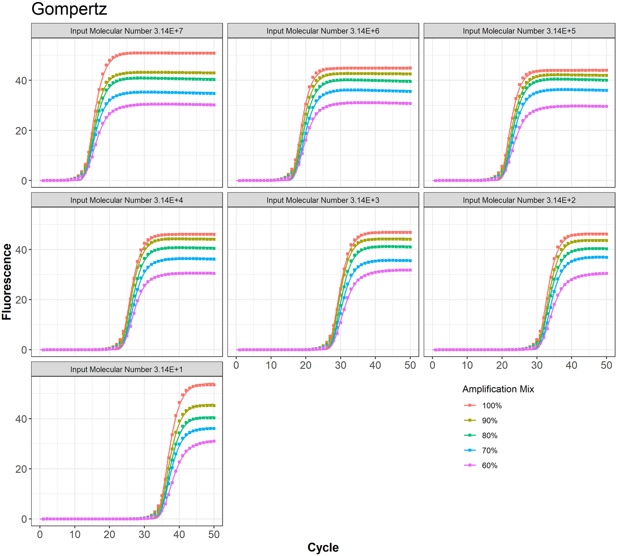
Gompertz model fit to the PCR data at different amplification mix for all 7 input molecular numbers.

Logistic model fit to the PCR data at different amplification mix for all 7 input molecular numbers

Richard model fit to the PCR data at different amplification mix for all 7 input molecular numbers.
For each combination of fluorescence intensity and input molecular number, the cycle elasticities of fluorescence using the 3-parameter TWW method have been given in Table 4. For instance, for the molecular number 3.14E + 7 using amplification mix of 100%, the cycle elasticity evaluated at the point of inflection is 5.91%. This indicates that at the point of inflection, a 1% increase in cycle number would increase the fluorescence intensity by 5.91%. When the cycle threshold
Values of elasticities at the point of inflection and at cycle

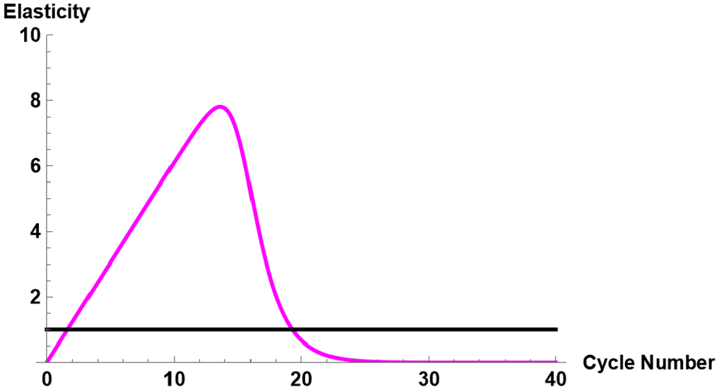
Cycle elasticity for molecular number 3.14E + 7 with amplification mix of 100%.
Table 5 shows the mean, SD, and 95% confidence interval for the fluorescence intensity for all 35 combinations of amplification mix and molecular number. The minimum value for the mean was 7.41, which belonged to 60% amplification mix and molecular number 3.14E + 1. The maximum was 35.32, which was associated with 100% amplification mix and molecular number 3.14 + 7.
Mean, standard deviation (SD), and 95% confidence interval (CI) for fluorescence.

In addition, a second set of publicly available qPCR data was analyzed using a 3-parameter TWW. 38 The results are given as a supplemental material. The fluorescence readings used were constructed for K1/K2 amplification for the average of 5 runs at 6 molecular numbers ranging from 4.17E + 7 to 4.17E + 2.
Discussion
In this article, we introduced a new 3-, 4-, and 5-parameter TWW growth model and applied the 3-parameter TWW model to analyze the qPCR data. The performance of this new model was then compared with Gompertz, logistic, and Richard models regarding model fit, precision, and efficiency. One advantage of the TWW model, when compared with the Richard model, is the capability of its 3 parameters to adequately estimate parameters with high efficiency and accuracy. The fewer the number of parameters used, the easier convergence is when using nonlinear regression fit. If the 3-parameter TWW model does not adequately fit the data, then one can try using the 4- or 5-parameter TWW model. In the analysis of the qPCR data used in this article, the 3-parameter TWW model showed a very high level of precision and relative efficiency as well as model fit when compared to the other models. A reliable estimate of cycle threshold has an utmost importance in diagnostic testing for detection of diseases, especially when monitoring infectious diseases.
A lack of consensus exists on how best to perform, interpret, and validate qPCR experiments. The problem is exacerbated by a lack of sufficient experimental detail in many publications, which impedes a reader’s ability to evaluate critically the quality of the results presented or to repeat the experiments. Following these guidelines would result in better experimental practice, allowing more reliable and unequivocal interpretation of qPCR results.39,40
To minimize the risk of errors and guarantee the reliability of laboratory results, quality control safeguards should be put in place. These measures may include regular tuning and upkeep of laboratory facilities, strict adherence to the laboratory standard protocol and procedures, and documentation of all processes. Following these measures will help reduce variability as well as increase precision, accuracy, and reliability. In addition, if the data quality control points toward the presence of outlier(s) or influential observation(s) in the data, one should not use the statistical method of least squares to estimate the model parameters. Instead, the usage of a robust nonlinear minimizer such as the method introduced by Tabatabai et al 41 should be used to estimate the model parameters.
Given the results shown herein, it may be feasible in a future study to use the
When applied for the purpose of amplification of molecular constituents and subsequent processing, such as DNA and mRNA production in preparation of a molecular candidate for nucleotide sequencing, the results suggest a feasible calibration and predictive capability to reach maximum yield given initial and final PCR target conditions. The reader may consider a case where a whole genome is to be sequenced or multiple fragments of RNA are to be sequenced for viral pandemic tracking.
The close agreement of the results to the model also suggests a means of detecting signal and cycle losses when comparing to a calibrated qPCR system using the TWW growth model, such as when inhibitors are present in biological samples as mentioned by Guescini. 35 A future work might include qPCR experiments for detection of various DNA/RNA of specific antigens of interest with controls.
Conclusions
We developed a family of 3-, 4-, and 5-parameter TWW growth models and compared the 3-parameter model with the classical models currently used in the analysis of qPCR. For the qPCR data that were analyzed in this article, we showed that the TWW model is a competitive model outperforming the Gompertz, logistic, and Richard models in model fit, precision, and relative efficiency and can be used as an alternative model in analyzing qPCR data. Supplementary R and Mathematica codes were included that would calculate the
Footnotes
Funding:
The author(s) disclosed receipt of the following financial support for the research, authorship, and/or publication of this article: The project has been supported by Meharry Medical College RCMI grant (NIH grant MD007586) and TN-CFAR (NIH grant 2P30 AI110527).
Declaration of conflicting interests:
The author(s) declared no potential conflicts of interest with respect to the research, authorship, and/or publication of this article.
Author Contributions
MT introduced the TWW growth model. MT, KPS, TLW, and DW wrote and edited the manuscript. Graphics, computations, and software programs were produced by MT and DW. All authors read and approved the final manuscript.