Sage Journals: Discover world-class research

Abstract

Genomic structural variations are significant causes of genome diversity and complex diseases. With advances in sequencing technologies, many algorithms have been designed to identify structural differences using next-generation sequencing (NGS) data. Due to repetitions in the human genome and the short reads produced by NGS, the discovery of structural variants (SVs) by state-of-the-art SV callers is not always accurate. To improve performance, multiple SV callers are often used to detect variants. However, most SV callers suffer from high false-positive rates, which diminishes the overall performance, especially in low-coverage genomes. In this article, we propose a post-processing classification–based algorithm that can be used to filter structural variation predictions produced by SV callers. Novel features are defined from putative SV predictions using reads at the local regions around the breakpoints. Several classifiers are employed to classify the candidate predictions and remove false positives. We test our classifier models on simulated and real genomes and show that the proposed approach improves the performance of state-of-the-art algorithms.

Keywords

Structural variation next-generation sequencing classification random forest support vector machines logistic regression

Introduction

Genome variations are one of the main causes of phenotypic variations as well as some complex diseases such as cancers, mendelian disorders, schizophrenia, autism, and many neurological disorders.^1,2 Genome variations are divided into 3 classes: single-nucleotide variants (SNVs), small insertions and deletions (indels), and genome structural variations. The latter refer to rearrangements in genome regions that are at least 50 bp long. These rearrangements have several forms including insertions, deletions, translocations, inversions, duplications, and copy number variations (CNVs).³

The advances of next-generation sequencing (NGS) have increased the interest in finding accurate structural variants (SVs). A typical SV detection approach includes 3 main stages: alignment of short reads to a reference genome, analysis of read alignments to find SV regions, and finally verification of putative SVs. Several NGS alignment tools are available for aligning NGS reads. These tools have different strategies and allow several alignment options.^4-6 The analysis of read alignments consists of finding paired-end reads with abnormal alignments, reads with subpart alignments, and read depth (RD). An abnormal/discordant read is a paired-end read that is not aligned as expected in the distance between its ends or orientation. Such reads are known as read-pair (RP) signatures and are used to specify the SV type and to approximate regions of breakpoints. Some read aligners, such as BWA-MEM⁷ and Bowtie2,⁸ support partial read alignment of reads that are difficult to map completely to a reference genome due to variants in the DNA sample, incomplete status of the reference genome, or sequencing errors. Therefore, clipped reads, reads with subpart alignments known as split reads (SRs), are one of the main sources of information used to refine SV breakpoints at low base pair resolution. The RD of a region is the average number of reads aligned to each base pair in that region. Read depth signatures are usually used to find CNVs as well as long deletions and duplications.

Initial strategies for finding SVs were based on using only one of the aforementioned signatures.^9-13 These approaches suffer from high false-positive rates, which decreases the performance of the SV caller. In fact, short reads, repeat regions in the human genome, and gaps in the reference genome cause ambiguity in read alignments. About 50% of the human genome contains repeats¹⁴ and the current human reference genome, GRCh38, contains 349 gaps with about 160 million total gap length.¹⁵ Consequently, some approaches use one signature for predicting SVs and the other signature for filtering. For example, some approaches use RP for SV prediction and SR for refining the predictions,^16,17 whereas other approaches use RD for prediction and RP signatures for verification.^18,19 Other approaches integrate multiple signatures and use scoring functions^20,21 or supervised learning for filtering.^22-24

In addition to the integration at signature level, some studies integrate and merge predictions from several SV callers. Different strategies have been applied for merging and filtering SV predictions including assembly-based refinements,^25,26 majority voting,²⁷ and algorithms’ priority as in MetaSV²⁶ which gives the SR approaches a higher priority than the RP approaches. Becker et al²⁸ use prior knowledge to train a statistical model for merging and filtering SV call sets from 8 SV calling algorithms. It is based on 2 discrimination features, namely, SV types and sizes. These approaches require running their default SV callers, usually 4 to 8, which is impractical and time-consuming. Accordingly, we provide a new data mining approach for post-processing SVs (PostSV) to filter SV calls from SR-based methods. PostSV is not like other approaches which are restricted to a specific set of SV calling algorithms. As Becker et al,²⁸ our solution based on using knowledge to filter SVs. PostSV is a classification based-approach for filtering deletions. Because most SV callers suffer from the high number of false positives in low-coverage samples,^17,24 PostSV has been designed to improve the performance of SV callers in detecting deletions from low-coverage genomes. In this article, we experimentally demonstrate that PostSV improves the performance of state-of-the-art approaches.

The Proposed Method: PostSV

Figure 1 shows an overview of PostSV, the proposed method for post-processing SVs. PostSV assumes that SV calls may be generated by one or multiple algorithms. The inputs for PostSV are the set of read alignments as a file in BAM format,²⁹ the reference genome as a file in FASTA format, and the SV predictions as a 3-tuple: chromosome name, start position, and end position. PostSV assumes that the read alignments are generated by a read aligner that supports partial read alignments, including BWA-MEM⁷ or Bowtie2.⁸ The following describes the proposed approach.

Figure 1.

The workflow of PostSV. SV stands for structural variant.

Preprocessing

During the preprocessing phase, SV predictions are combined by keeping 1 copy of the duplicate predictions. Two predictions are duplicate if they have the same location (start and end positions). Then, the BAM file is parsed to extract clipped reads at local regions of SV breakpoints. A clipped read alignment is a read end that is partially aligned. Clipped reads have been used to specify accurate breakpoints.³⁰ We assume that a read that spans an SV breakpoint is aligned with clipped portions, as shown in Figure 2. A read may be clipped from the left side, the right side, or both. 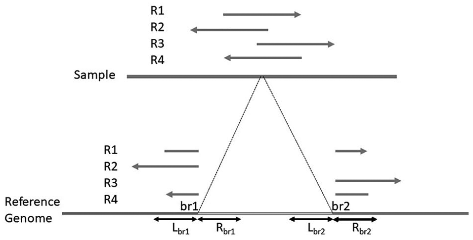A read that overlaps the breakpoint of a deletion may have several alignment states: the left subpart aligned at $b r 1$ and the right subpart aligned at $b r 2$ , such as $R 1$ and $R 4$ in Figure 2; one part aligned at one of the breakpoints and the other aligned at an incorrect location; and one part aligned at one of the breakpoints and the other portion not aligned, such as $R 2$ and $R 3$ . The reads of the first one of these alignment states are called single-read signatures.

Figure 2.

Clipped reads and single-read signatures at the deletion’s breakpoints.

For each SV prediction, the clipped reads that overlap the local region of the SV breakpoints are mapped to the rearranged breakpoint region, which is constructed by applying SVs to the breakpoint regions. A local alignment algorithm (Smith-Waterman)³¹ is used to align the read sequences. For each read alignment, the alignment score is computed and normalized by dividing the pairwise sequence alignment score by the sequence length. We choose the maximum score for each SV prediction that has multiple clipped reads. However, not every SV prediction has clipped reads at its breakpoints. Similarly, we compute an alignment score for each single-end signature, assuming that they are SV predictions. These alignment scores are used to resolve breakpoints and later to extract features.

The breakpoints of the SV predictions are resolved using single-read signatures. The orientation and order of the read that forms the deletion’s signature are preserved such that both read parts are mapped on the same strand and the left part of the read aligns before the right part. A prediction’s breakpoints are updated using single-end signature breakpoints if the following conditions are satisfied: (1) there is a single-end deletion signature that is overlapping an SV region; (2) the distance between the breakpoints of a single-end signature and the corresponding SV breakpoints does not exceed a defined threshold (250 bp is defined as the default); and (3) the alignment score of deletion signature is higher than that of the clipped reads at the SV breakpoints.

Feature extraction

Given locations of SV predictions, the set of read alignments as a BAM-formatted file,²⁹ and the reference genome as a FASTA-formatted file, the candidate SV is annotated with 30 binary features based on RP, clipped reads, and RD at the breakpoints.

Read pair–based features

Most SV callers use the RP signatures for identifying candidate SV regions. A deletion’s RP signature is a paired-end read with both read ends mapped on the same reference sequence (same chromosome) and has an insert size more than the expected insert size (IS), which is the number of bases from the leftmost mapped base to the rightmost mapped base. The insert size of a normal paired-end read should be between minimum and maximum thresholds $(μ_{I S} \pm n σ_{I S})$ , where $µ_{I S}$ and $σ_{I S}$ are the mean and standard deviation of insert size, respectively, and $n$ is the number of standard deviation from the mean, where the default value for n is 3. Figure 3 illustrates RP signatures for a deletion. The deletion signatures for the predictions are extracted from the BAM file. It is assumed that the RP supports an SV if the distance between the SV’s breakpoints and the corresponding RP signature breakpoints is within a defined threshold, where the default distance is 500 bp. We define 2 features for each SV prediction. One feature is for the existence of an RP signature that supports the SV prediction. The second feature is equal to 1 if the number of RP signatures does not exceed a defined threshold; otherwise, it is set to 0. The genome’s mean coverage is used as the default threshold.

Figure 3.

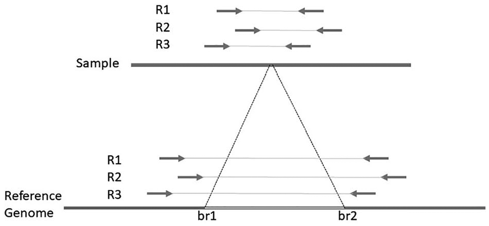
Read-pair signatures supporting deletion.

Read depth–based features

The RD is an important signature for identifying deletions, duplications, and CNVs. Accordingly, the RDs of the local regions around breakpoints are used to define features. We compute the RD of 4 regions: the left region of the start breakpoint $L_{b r 1}$ , the right region of the start breakpoint $R_{b r 1}$ , the left region of the end breakpoint $L_{b r 2}$ , and the right region of the end breakpoint $R_{b r 2}$ . Figure 3 illustrates these regions. The default length of each region is 50 bp. The RD of a region is the average number of reads that are aligned to each base in the region. Using the mean depth of the genome and the RD of the 4 local regions ( $L_{b r 1}$ , $R_{b r 1}$ , $L_{b r 2}$ , and $R_{b r 2}$ ), 16 features are defined. For each of the 4 local regions, 4 features are defined that represent the state of the RD. The first state is for homozygous deletion, for which the RD of the region is expected to be nearly zero. The second is for heterozygous deletion, for which the RD is more than zero and up to half of the mean depth. The third is for the normal region, in which the RD is nearly equal to the mean genome coverage. The fourth represents RDs that are more than the mean coverage of the genome.

Clipped read–based features

As stated earlier, clipped reads are used to define features. Each SV prediction has an alignment score computed from the clipped reads at its breakpoint regions. Some SV predictions do not have clipped reads. Therefore, we define a feature with a value of 1 for predictions without clipped reads. The alignment scores are rounded to the tenths and used to define 11 features that are representing alignment score levels $(0, 0.1, 0.2, \dots, 1)$ .

The 30 features are combined into 1 matrix. The rows of this matrix represent the SV predictions, and the columns represent the features. We use the Phi coefficient³² to measure the associations among attributes. If there are highly correlated attributes with an absolute correlation $0.75$ , the attribute with the largest mean absolute correlation is ignored. Accordingly, 3 features are removed. Each row is labeled according to whether the prediction is an actual variant or not. The final matrix is used to train and test classifier models.

Classification

Classification of SV predictions into true positives and false positives were explored using 3 different machine learning algorithms, namely, random forest (RF), support vector machine (SVM), and logistic regression (LR). Random forest was introduced by Breiman³³ for classification and regression. It is an ensemble of classification trees (bagging)³⁴ in which each tree is built using a bootstrap sample of the training samples and a random selection of features at each split. A bootstrap sampling generates a new training dataset $S_{i}$ from the original training dataset $S$ . The samples in $S_{i}$ are selected randomly from $S$ . The size of $S_{i}$ is the same as $S$ . Thus, some samples in $S$ may be selected many times and some samples may not be selected. In bagging, a predefined number $n$ of bootstrap samples $S_{1}, S_{2}, . ., S_{n}$ are generated. In the original RF,³³ attributes are randomly selected at each node. The number of chosen attributes is $⌊ l o g_{2} (a) ⌋ + 1$ , where $a$ is the number of attributes in the dataset. To build RF, a decision tree is built for each bootstrap $S_{i}$ . The total number of trees is $n$ . For classifying a new sample, a prediction is made by a majority vote of the $n$ trees while averaging their outputs in regression.

Support vector machine is one of the most popular supervised learning algorithms. They were proposed by Cortes and Vapnik³⁵ for binary classification. The main idea of an SVM is to separate samples with a hyperplane that maximizes the margins between them. Logistic regression is a statistical approach for binary classification.³⁶ The main purpose of LR is to analyze the interaction between attributes (predictors) and the class attribute (response or dependent).

Experimental Results and Discussion

We use simulated datasets to train RF, SVM, and LR classifiers for differentiating between true positives and false positives of a set of deletion predictions. This set is assumed to be generated by an SR-based SV caller. As some of the features are extracted from clipped reads at breakpoint regions, PostSV is designed to filter predictions generated by SR-based approaches.

To generate training examples, we introduce random structural variations into a copy of hg19 using RSVsim,³⁷ an SV simulator. The number of variations is 1000 deletions, 1000 inversions, 500 insertions, and 1000 tandem duplications (Supplementary File 1). After that, we generate paired-end reads from the altered genome by wgsim.³⁸ The reads have an insert size of 250 bp with 75 bp read length and 0.001 base error rate. The genome has low coverage 5×. The read aligner BWA-MEM is used to align paired-end reads to the reference genome. Then, the training predictions are generated using 3 SV callers, namely, DELLY,¹⁶ SoftSV,¹⁷ and SVelter.²¹ We combine their predictions, and we remove duplicates. For each prediction, the clipped reads that overlap the local region of one of the breakpoints are extracted. The local region of a breakpoint is the region on the left and right of the breakpoint, and we use 25 bp at the left and right for breakpoints as a cutoff distance for the local region. SAMtools²⁹ is used to extract the regions required for constructing rearranged breakpoint regions. The training samples are labeled. As SR-based callers are supposed to specify SV breakpoints at base pair resolution, it is assumed that the prediction is a positive example if it overlaps one of the ground truth regions and the distance between the prediction breakpoints and the actual breakpoints does not exceed 50 bp. Accordingly, the training set consists of 2728 positive examples and 1817 negative examples.

To evaluate the performance of the proposed approach, we generate 6 simulated samples in the same way as the training sample. We simulate 2000 SVs: 500 deletions, 500 inversions, 500 insertions (interspersed duplication and translocations), and 500 tandem duplications (Supplementary File 2). The SVs’ sizes are between 50 bp and 10 kbp and the same SVs are used as testing samples. The insert size for all testing samples is 500 bp. We use different sequencing settings in coverage (5× and 10×) and read length (75, 100, and 150). In addition, we test our approach on the real sample NA12878. This sample is chosen because it has high-quality benchmark SV calls.³⁹ The alignments of the low-coverage sample are obtained from the 1000 Genomes Project.⁴⁰ The sample has approximately 6× coverage mean and a read length of 101 bp. As our simulated samples, the alignments of the real sample were generated by the BWA-MEM aligner.

Using the training dataset, we trained 3 classifier models: RF, SVM, and LR on the same dataset. We apply PostSV to filter SV predictions generated by 3 SV callers, namely, DELLY, SoftSV, and SVelter, over the testing dataset.

Results on a simulated dataset

The SV callers were executed using their default settings. We evaluate the effect of resolving breakpoints over simulated samples. Table 1 shows the effect of resolving breakpoints for training prediction. The performance regarding F-score is increased by 3% for DELLY and SVelter, and the results show no effect on SoftSV. In the same way, we evaluate the testing samples. The results reveal that the overall performance has increased by 2% and 3% for DELLY and SVelter, respectively. However, resolving breakpoints is effective for samples with coverage 5× as the overall F-score has improved by 3% and 5% for DELLY and SVelter, respectively. In contrast, resolving breakpoints has no significant improvement over samples with 10× coverage. Figure 4 shows the comparison of the effect of resolving breakpoints and applying classifiers for testing samples. The details for individual genomes are available in Supplementary File 3.

Table 1.

Performance of detecting deletions on the training sample after resolving breakpoints.

SV Caller	Sensitivity	Precision	F-Score
DELLY	0.808	0.591	0.683 (+3%)
SoftSV	0.665	0.640	0.652 (+0%)
SVelter	0.639	0.605	0.622 (+3%)

Abbreviation: SV, structural variant.

Figure 4.

The F-score, sensitivity, and precision over testing simulated samples.

In general, the 3 classifiers achieve comparable performance with an average F-score increase of about 17% for DELLY, 13% for SoftSV, and 18% for SVelter (Figure 4). The sensitivity of both DELLY and SoftSV has decreased by 8% and 9%, whereas that of SVelter shows a 2% increase. The precision has increased across the 3 SV callers by about 39% (DELLY), 34% (SoftSV), and 45% (SVelter).

The average improvement of using classifiers on DELLY’s samples that have coverage 5× is the same as that over samples with coverage 10×. This is because the numbers of false positives over the 2 groups are the same. On the other hand, the percentage of false positives changes with increasing coverage for SoftSV and SVelter by 26% and 55%, respectively. Thus, the performance of the classifiers is higher on samples of coverage 10× than on samples of 5× coverage.

Results on a real dataset

In addition to simulated datasets, PostSV is applied to the real sample NA12878. The numbers of predictions that are produced by SV callers are 6612 (DELLY), 1797 (Soft S), and 3926 (SVelter). The F-score of using SV callers only (ie, before using PostSV) are 0.273 for DELLY, 0.404 for SoftSV, and 0.268 for SVelter. Table 2 shows how resolving breakpoints affects the performance of SV callers. Notably, resolving breakpoints has no significant improvement for SoftSV, whereas the performance of DELLY and SVelter has improved. This is probably due to the fact that DELLY and SVelter compute the breakpoints in some cases, whereas SoftSV depends on clipped reads provided by the aligner. However, this is confirmed with the results on a simulated dataset. Table 3 shows the comparison of the results of applying RF, SVM, and LR to the predictions of SV callers. The F-score of DELLY and SVelter has increased, where that for SoftSV slightly decreased. However, the precision of SoftSV has increased by about 19% (RF), 21% (SVM), and 25% (LR). The RF classifier tends to be more sensitive than the other classifiers. This is at the cost of precision, whereas SVM and LR produce higher precision than RF. The difference between the improvement percentages over SV callers depends on the number of predictions and the number of false positives in the sample.

Table 2.

Performance of detecting deletions on the real sample NA12878 after resolving breakpoints.

SV Caller	Sensitivity	Precision	F-Score
DELLY	0.556	0.218	0.313 (+4%)
SoftSV	0.342	0.498	0.405 (+0%)
SVelter	0.378	0.250	0.301 (+3%)

Abbreviation: SV, structural variant.

Table 3.

Performance of detecting deletions on the real sample NA12878 using classifier models.

Classifier	SV Caller	Sensitivity	Precision	F-Score
RF	DELLY	0.396 (−9%)	0.614 (+42%)	0.482 (+21%)
	SoftSV	0.274 (−7%)	0.680 (+19%)	0.390 (−1%)
	SVelter	0.300 (−4%)	0.495 (+27%)	0.374 (+11%)
SVM	DELLY	0.362 (−12%)	0.722 (+53%)	0.482 (+21%)
	SoftSV	0.265 (−8%)	0.702 (+21%)	0.385 (−2%)
	SVelter	0.250 (−9%)	0.637 (+41%)	0.359 (+9%)
LR	DELLY	0.371 (−11%)	0.734 (+54%)	0.493 (22%)
	SoftSV	0.251 (−9%)	0.746 (+25%)	0.376 (−3%)
	SVelter	0.246 (−9%)	0.632 (+41%)	0.355 (+9%)

Abbreviations: LR, logistic regression; RF, random forest; SV, structural variant; SVM, support vector machine.

In this study, each of the 3 SV callers is applied to 7 testing genomes (6 simulated and 1 real). Thus, each classifier is applied to 21 samples (7 samples from each SV callers). The mean F-score over all samples before applying the classifiers is 0.594. The mean F-scores after applying RF, SVM, and LR are 0.740, 0.745, and 0.746, respectively. An independent-samples t test was conducted to compare F-scores for SV callers before and after applying PostSV. The results indicate a significant improvement in F-score ( $P < . 001$ for all classifiers). There were no statistically significant differences between the F-score means of classifiers as determined by 1-way analysis of variance (ANOVA; $P > . 05$ ).

Conclusions

In this article, a post-processing method is proposed to improve the performance of SV callers in low-coverage samples. The method uses clipped reads for resolving SV breakpoints. This is a new approach for annotating SV predictions based on coverage, SRs, and rearrangement of breakpoint regions. A simulated dataset is used to train RF, SVM, and LR models to classify predictions into true positives and false positives. The proposed method is intended to handle SV predictions generated by SR-based approaches. We apply the classifier models to predictions generated by 3 SV callers, namely, DELLY, SoftSV, and SVelter, using simulated and real genomes. The results show that the performance of the 3 classifiers is comparable and can be used to improve SV classification regarding precision and F-score. Although a simulated dataset is used in training the models, the results are promising, and the availability of a benchmark from real samples would improve solutions for SV detection.

Supplemental Material

supFile1_xyz2852972714ee4 – Supplemental material for PostSV: A Post–Processing Approach for Filtering Structural Variations

Supplemental material, supFile1_xyz2852972714ee4 for PostSV: A Post–Processing Approach for Filtering Structural Variations by Eman Alzaid and Achraf El Allali in Bioinformatics and Biology Insights

Supplemental Material

supFile2_xyz285298d9ad6d3 – Supplemental material for PostSV: A Post–Processing Approach for Filtering Structural Variations

Supplemental material, supFile2_xyz285298d9ad6d3 for PostSV: A Post–Processing Approach for Filtering Structural Variations by Eman Alzaid and Achraf El Allali in Bioinformatics and Biology Insights

Supplemental Material

supFile3_xyz285295dda35d1 – Supplemental material for PostSV: A Post–Processing Approach for Filtering Structural Variations

Supplemental material, supFile3_xyz285295dda35d1 for PostSV: A Post–Processing Approach for Filtering Structural Variations by Eman Alzaid and Achraf El Allali in Bioinformatics and Biology Insights

Footnotes

Acknowledgements

The authors gratefully acknowledge the use of the service of “SANAM” supercomputer at “King Abdulaziz City for Science and Technology” (KACST), Saudi Arabia. The authors also thank Prof Hatim Abo AlSamh for the useful discussions at initial stages of this work.

Funding:

The author(s) disclosed receipt of the following financial support for the research, authorship, and/or publication of this article: This research project was supported by a grant from the “King Abdulaziz City for Science and Technology” (KACST), Saudi Arabia (Grant No.1-17-02-001-0024).

Declaration of Conflicting Interests:

The author(s) declared no potential conflicts of interest with respect to the research, authorship, and/or publication of this article.

Author Contributions

EA and AE conceived of the project. EA designed and implemented the work. AE helped in the design and provided expert input. All authors read and approved the final manuscript.

ORCID iDs

Eman Alzaid

Achraf El Allali

Supplemental Material

Supplemental material for this article is available online.

References

Mitelman

Johansson

Mertens

The impact of translocations and gene fusions on cancer causation. Nat Rev Cancer. 2007;7:233-245.

Stankiewicz

Lupski

JR.

Structural variation in the human genome and its role in disease. Annu Rev Med. 2010;61:437-455.

Alkan

Coe

Eichler

EE.

Genome structural variation discovery and genotyping. Nat Rev Genet. 2011;12:363-376.

Homer

A survey of sequence alignment algorithms for next-generation sequencing. Brief Bioinform. 2010;11:473-483.

Reinert

Langmead

Weese

Evers

DJ.

Alignment of next-generation sequencing reads. Annu Rev Genomics Hum Genet. 2015;16:133-151.

Thankaswamy-Kosalai

Sen

Nookaew

Evaluation and assessment of read-mapping by multiple next-generation sequencing aligners based on genome-wide characteristics. Genomics. 2017;109:186-191.

Aligning sequence reads, clone sequences and assembly contigs with BWA-MEM. arXiv preprint arXiv:1303.3997; 2013.

Langmead

Salzberg

SL.

Fast gapped-read alignment with Bowtie 2. Nat Methods. 2012;9:357-359.

Chen

Wallis

McLellan

, et al. BreakDancer: an algorithm for high-resolution mapping of genomic structural variation. Nat Methods. 2009;6:677-681.

10.

Hormozdiari

Alkan

Eichler

Sahinalp

SC.

Combinatorial algorithms for structural variation detection in high-throughput sequenced genomes. Genome Res. 2009;19:1270-1278.

11.

Schulz

Long

Apweiler

Ning

Pindel: a pattern growth approach to detect break points of large deletions and medium sized insertions from paired-end short reads. Bioinformatics. 2009;25:2865-2871.

12.

Xie

Tammi

MT.

CNV-seq, a new method to detect copy number variation using high-throughput sequencing. BMC Bioinformatics. 2009;10(1):80.

13.

Abyzov

Urban

Snyder

Gerstein

CNVnator: an approach to discover, genotype, and characterize typical and atypical CNVs from family and population genome sequencing. Genome Res. 2011;21:974-984.

14.

Treangen

Salzberg

SL.

Repetitive DNA and next-generation sequencing: computational challenges and solutions. Nat Rev Genet. 2012;13:36-46.

15.

Schneider

Graves-Lindsay

Howe

, et al. Evaluation of GRCh38 and de novo haploid genome assemblies demonstrates the enduring quality of the reference assembly. Genome Res. 2017;27:849-864.

16.

Rausch

Zichner

Schlattl

Stütz

Benes

Korbel

JO.

DELLY: structural variant discovery by integrated paired-end and split-read analysis. Bioinformatics. 2012;28:i333-i339.

17.

Bartenhagen

Dugas

Robust and exact structural variation detection with paired-end and soft-clipped alignments: SoftSV compared with eight algorithms. Brief Bioinform. 2016;17:51-62.

18.

Medvedev

Fiume

Dzamba

Smith

Brudno

Detecting copy number variation with mated short reads. Genome Res. 2010;20:1613-1622.

19.

Zhao

inGAP-sv: a novel scheme to identify and visualize structural variation from paired end mapping data. Nucleic Acids Res. 2011;39:W567-W575.

20.

Chen

Schulz-Trieglaff

Shaw

, et al. Manta: rapid detection of structural variants and indels for clinical sequencing applications. 15;32:1220-1222. 2016.

21.

Zhao

Emery

Myers

Kidd

Mills

RE.

Resolving complex structural genomic rearrangements using a randomized approach. Genome Biol. 2016;17: 126.

22.

Michaelson

Sebat

forestSV: structural variant discovery through statistical learning. Nat Methods. 2012;9:819-821.

23.

Kronenberg

Osborne

Cone

, et al. Wham: identifying structural variants of biological consequence. PLoS Comput Biol. 2015;11:e1004572.

24.

Alzaid

Allali

Aboalsamh

Classification approach for genome structural variations detection. J Proteomics Bioinform. 2018;11:211-218.

25.

Wong

Keane

Stalker

Adams

DJ.

Enhanced structural variant and breakpoint detection using SVMerge by integration of multiple detection methods and local assembly. Genome Biol. 2010;11:R128.

26.

Mohiyuddin

, et al. MetaSV: an accurate and integrative structural-variant caller for next generation sequencing. Bioinformatics. 2015;31:2741-2744.

27.

Lam

Pan

Clark

, et al. Detecting and annotating genetic variations using the HugeSeq pipeline. Nat Biotechnol. 2012;30:226-229.

28.

Becker

Lee

Leone

, et al. FusorSV: an algorithm for optimally combining data from multiple structural variation detection methods. Genome Biol. 2018; 19:38.

29.

Handsaker

Wysoker

, et al. The sequence alignment/map format and SAMtools. Bioinformatics. 2009;25:2078-2079.

30.

Guan

Sung

WK.

Structural variation detection using next-generation sequencing data: a comparative technical review. Methods. 2016;102:36-49.

31.

Smith

Waterman

MS.

Identification of common molecular subsequences. J Mol Biol. 1981;147:195-197.

32.

Pearson

K. I.

Mathematical contributions to the theory of evolution—VII. On the correlation of characters not quantitatively measurable. Philos T R Soc Lond. 1900;195:1-47.

33.

Breiman

Random forests. Mach Learn. 2001;45:5-32.

34.

Breiman

Classification and Regression Trees. Abingdon, UK: Routledge; 2017.

35.

Cortes

Vapnik

Support-vector networks. Mach Learn. 1995;20:273-297.

36.

Grimm

Yarnold

PR.

Reading and Understanding Multivariate Statistics. Washington, DC: American Psychological Association; 1995.

37.

Bartenhagen

Dugas

RSVSim: an R/Bioconductor package for the simulation of structural variations. Bioinformatics. 2013;29:1679-1681.

38.

Heng

WGsim-read simulator for next generation sequencing. Github Repository. https://github.com/lh3/wgsim. Updated 2011.

39.

Parikh

Mohiyuddin

Lam

, et al. svclassify: a method to establish benchmark structural variant calls. BMC Genomics. 2016;17:64.

40.

Zheng-Bradley

Streeter

Fairley

, et al. Alignment of 1000 genomes project reads to reference assembly GRCh38. Gigascience. 2017;6(7):1-8.

Supplementary Material

Please find the following supplemental material available below.

For Open Access articles published under a Creative Commons License, all supplemental material carries the same license as the article it is associated with.

For non-Open Access articles published, all supplemental material carries a non-exclusive license, and permission requests for re-use of supplemental material or any part of supplemental material shall be sent directly to the copyright owner as specified in the copyright notice associated with the article.

0.00 MB

0.39 MB

0.23 MB

0.03 MB