Sage Journals: Discover world-class research

Abstract

Restricted mean survival time (RMST), recommended for reporting survival, lacks a tool to evaluate multilevel factors. The potential of the Gini’s mean difference of RMSTs (Δ) is explored in a comparison of a lymph node ratio-based classification (LNRc) versus a number-based classification (ypN) applied to stage II/III breast cancer patients who received neoadjuvant chemotherapy and underwent axillary dissection. Number of positive nodes (npos) classified patients into ypN0, npos = 0, ypN1, npos = [1,3], ypN2, npos = [4,9], and ypN3, npos ⩾ 10. Ratio npos/(number of nodes examined) of 0, (0,0.20], (0.20,0.65], and >0.65, classified patients into Lnr0 to Lnr3, respectively. Unadjusted and Cox-adjusted RMSTs were computed for the ypN and LNRc’s. At a follow-up time horizon of 72 months for 114 node-negative and 254 node-positive patients, unadjusted ypN0-ypN3 RMSTs were 62.4-41.4 months, Δ = 11.9 months (95%CI: 7.4-16.9), and Lnr0-Lnr3 62.4 to 36.3 months, Δ = 14.0 months (95%CI: 10.1-18.1). Cox models’ ypN1-ypN3 hazard ratios were 1.81-3.30, and Lnr1-Lnr3 1.52-4.39. Δ from Cox-fitted survival were ypN 8.1 months (95%CI: 5.9-10.5), LNRc 10.5 months (95%CI: 8.4-12.8). In conclusion, Gini’s mean difference is applicable to well established data in keeping with the literature on LNRc. It provides an alternative view on the improvement gained with a lymph node ratio-classification over using a number-classification.

Keywords

Dispersion information value predictive models regression analysis separation

Introduction

Restricted mean survival time (RMST) is the expected remaining life from the time origin to a specified time horizon, discounting future years beyond the horizon. A growing literature proposes RMST as the reference survival metric that clinical trials should report.^1,2 Almost all studies note its advantage over conventional metrics such as the hazard ratio or the median survival time. Incorporating RMST in the standard reporting of clinical trials will potentially supply more meaningful information to patients, physicians, and policymakers.³ Tools to compute the RMST are widely available. Simply, the RMST is the area below the survival curve, up to the specified time horizon. The difference ΔRMST between 2 survival curves is the area between the curves.⁴ When comparing 2 groups, ΔRMST (“delta method”) streamlines the survival analyses, allowing coherent comparisons. Authors have observed that ΔRMST outperformed the logrank test.⁵

However, ΔRMST has an impediment. Published studies have limited ΔRMST to the comparison of 2 arms. No allowance has been made to extend tests of RMSTs beyond 2 groups. That prevents its application to observational studies where prognostic factors can involve multiple levels, such as 13 histopathology classes in a cervical cancer study.⁶ Further developments are needed.

We argue that Gini’s mean difference is applicable to generalize ΔRMST. Gini’s mean difference for a set of quantities is defined as the average of the differences between all pairs of the quantities (La differenza media tra più quantità).⁷ For a factor with multiple levels, the quantities of interest are the RMST’s of the levels. Thus, Gini’s mean difference represents the average of all RMST’s differences between the factor’s levels, making it a general measure of the prognostic value of that factor.

In breast cancer, axillary lymph node management after neoadjuvant chemotherapy remains a large debate. Using data from a prospective Korean trial,^8,9 the present study applies Gini’s mean difference to assess the survival separation according to the numbers of involved lymph nodes retrieved from axillary dissection after neo-adjuvant therapy, denoted number-based classification (ypN), versus the survival separation according to the ratios of the involved nodes, denoted ratio-based classification (LNRc). The study will also evaluate well-known indices of prognostic models.

Methods

Patients

As reported previously,⁸ the patients were enrolled between March 2002 and September 2008 in a prospective trial of neoadjuvant chemotherapy. The study protocol had been reviewed and approved by the institutional review board at the Seoul National University Hospital. Recommendations of the Declaration of Helsinki for biomedical research involving human subjects were also followed. Informed consent was obtained for all patients. Patients had pathologically confirmed breast cancer, clinical stage II or III (AJCC 6th edition), measurable tumor, ECOG performance 0 to 2, no previous cancer therapy, and adequate bone marrow, hepatic, cardiac, and renal function. The patients underwent clinical examination, breast mammograms and ultrasound, computed tomography (CT) of the chest, bone scan, and breast magnetic resonance imaging (MRI). Tumor size was measured on MRI.

Neoadjuvant chemotherapy consisted of docetaxel and doxorubicin, after which the patients underwent curative surgery, either lumpectomy or mastectomy, and axillary lymph node dissection. Three cycles of post-operative docetaxel and doxorubicin were delivered, followed by radiation therapy if indicated according to the 2001’s American Society Clinical guidelines.¹⁰ Adjuvant hormone therapy was given to hormone receptor positive patients with 5 years tamoxifen or aromatase inhibitor.

Survival analyses

Data included patient’s demographic, clinical, and pathologic factors. Estrogen receptor (ER), progesterone receptor (PR), HER2, p53, bcl2, ki-67, and EGFR were assessed on pre-chemotherapy tissue specimens. Lymph nodes removed by surgery were assessed by hematoxylin and eosin-stained sections.

The number-based classification (ypN) categorized the lymph nodes according to the number of involved (positive) nodes npos as follows: ypN0, npos = 0; ypN1, npos = 1 to 3; ypN2, npos = 4 to 9; ypN3, npos ⩾ 10.

The ratio-based classification (LNRc) categorized the lymph nodes according to the ratio npnx = npos/(number of nodes examined) as follows: Lnr0, npnx = 0; Lnr1, npnx > 0 and ⩽0.20; npnx > 0.20 and ⩽0.65; npnx > 0.65.

The prognostic effects of ypN and LNRc were compared in univariate and multivariate models. Disease-free survival (DFS) was the outcome of interest. The observation time was from the date of surgery to last follow-up or event if it occurred first. Event was death from any cause, or first distant, regional or local recurrence, or any new primary, contralateral breast cancer or other malignant tumor. Univariate survival analyses used the life-table method.¹¹ Comparisons of the levels of ypN or LNRc used the logrank test¹¹ and the RMST restricted mean survival times.⁴ Gini’s mean difference was applied to the RMSTs as detailed farther below.

Combining ypN and LNRc was explored by subclassifying ypN categories with LNRc—asking the question, among subgroups of ypN patients, do survival differ according to LNRc—and conversely subclassifying LNRc categories with ypN—asking whether among subgroups of LNRc, do survival differ or not according to ypN.

Confounder model

Multivariate analyses used the Cox proportional hazards regression model. A “confounder model” was established,¹² selecting covariates by forward and backward regression using the Akaike Information Criterion, without the ypN and LNRc variables. Covariates scanned for inclusion in the confounder model were age, weight, height, body mass index (BMI), primary tumor inflammatory status, adjuvant hormonal therapy, type of surgery, radiation therapy, initial tumor, preoperative T- and N-stage, postoperative ypT stage, ECOG status, pathologic complete response pCR, status of HER2, ER, PR, p53, bcl2, and EGFR, ki-67, tumor subtype, nuclear and histological grade. Missing data regarding initial tumor size, ypT, p53, bcl2, ki-67, and EGFR were imputed by Multivariate Imputations by Chained Equations.¹³ Multivariate fractional polynomial regression assessed whether covariates needed a non-linear transform.¹⁴

Prognostic indices

The multivariate utility of ypN or LNRc were assessed by the change of Cox models’ indices when either ypN or LNRc were added as covariates to the confounder model. Gini’s mean difference was applied to RMSTs of the ypN or LNRc fitted survivals. Other indices considered in the study were as follows:

AIC, Akaike Information Criterion, the value of a model’s log likelihood with an added penalty for the number of parameters in the model.

R2N, Nagelkerke’s index, a measure of explained randomness and overall performance of a model.¹⁵

D, Royston-Sauerbrei’s measure of prognostic separation.¹⁶

R2D, Royston-Sauerbrei’s index of explained variation.¹⁶

C-index, concordance between models based on ranking.¹⁷

NRI, Net Reclassification Improvement, estimates the net fraction of reclassifications in the right direction by making decisions based on predictions with a marker, compared to decisions without the marker.¹⁵

Gini’s mean difference

Noting X₁, . . ., X_n the set of n ordered values of the RMST’s, X₁ ⩽ . . . ⩽ X_n, Gini’s mean difference,^7,18 here denoted Δ, may be written as

\begin{matrix} Δ = \frac{1}{n (n - 1)} \sum_{i = 1}^{n} \sum_{j = 1}^{n} | X_{i} - X_{j} | (i \neq j) \end{matrix}

(1)

which can also be computed as

\begin{matrix} Δ = \frac{2}{n (n - 1)} \sum_{i = 1}^{n} (2 i - n - 1) X_{i} . \end{matrix}

(2)

The following is not required to compute Δ but is useful to understand that Δ is the average of the differences.¹⁹ Writing Δ_ij the difference between a pair of observations X_i and Xj

\begin{matrix} Δ_{i j} = | X_{i} - X_{j} | (i \neq j), \end{matrix}

(3)

then the average of the absolute deviations of all X_j observations about each X_i is

\begin{matrix} Δ_{i} = \frac{1}{(n - 1)} \sum_{j = 1}^{n} | X_{j} - X_{i} | (i \neq j), \end{matrix}

(4)

discounting the deviation of an observation with itself, hence (n-1) in the denominator. Recalling that there are n distinct observations, the average of the Δ_i is

\begin{matrix} \frac{1}{n} \sum_{i = 1}^{n} Δ_{i} \end{matrix}

(5)

which, by replacing the Δ_i in (5) with its value from (4)

\begin{array}{l} = \frac{1}{n (n - 1)} \sum_{i = 1}^{n} \sum_{j = 1}^{n} Δ_{i j} (i \neq j) \\ = Δ \end{array}

showing that Δ is the average of all differences between all pairs of observations, not counting the difference of an observation with itself. Note that when n = 2, Δ is exactly ΔRMST mentioned in the introduction, that is, ΔRMST is an instance, ergo the introduction’s proposition that Gini’s mean difference generalizes ΔRMST. Note also from expression (1) or (2) that the unit of Δ is the same as the X quantities.

Software

Computations used R version 3.6.3, with packages survival (RMST, Cox regression, C-index), mfp (fractional polynomials), mice (multiple imputation), MASS (stepAIC), bootStepAIC, Hmisc (NRI). Confidence intervals of Gini’s mean differences were computed by 1000 bootstrap resamplings of the RMST’s. Gini’s mean difference, R2N, D, and R2D were computed using in-house scripts.

Results

Table 1 summarizes the characteristics of 368 patients who underwent axillary dissection. The overall median follow-up was 43.8 months (interquartile range 31.7-54.1 months). The study accrued more patients than earlier reported, but the distribution of characteristics did not change.^8,20 Patients were young, 69.8% (257 of 368) were younger than 50. Few were overweight. Most had T2-3 tumor and N1-2 nodal stage. Generally, surgery was mastectomy, and ⩾10 lymph nodes were excised. Negative hormone receptor status was more frequent than positive status. Radiation therapy was given to most patients. The type of first recurrence was predominantly distant, followed by regional then local recurrence.

Table 1.

Patients’ Characteristics.

Characteristic	Total (N)	Node-negative (%)	Node-positive (%)	Characteristic	Total (N)	Node-negative (%)	Node-positive (%)
	Total (N)	N = 114	N = 254	Characteristic	Total (N)	Node-negative (%)	Node-positive (%)
	N = 368	31.0%	69.0%
Age, years				Number of nodes excised
<40	103	39.8	60.2	1-3	7	42.9	57.1
41-49	154	27.3	72.7	4-9	69	34.8	65.2
50+	111	27.9	72.1	10+	292	29.8	70.2
Body weight, kg				ypN-stage
<50	44	29.5	70.5	ypN0: 0 positive nodes	114	100	0
50-64	239	30.1	69.9	ypN1: 1-3	114	0	100
65+	85	34.1	65.9	ypN2: 4-9	89	0	100
Height, m				ypN3: 10+	51	0	100
<1.55	89	34.8	65.2	LNR-stage
1.55-1.60	157	25.5	74.5	Lnr0 = pN0	114	100	0
>1.60	122	35.2	64.8	Lnr1: 0.01-0.20	93	0	100
BMI, kg/m²				Lnr2: 0.21-0.65	98	0	100
⩽20	52	36.5	63.5	Lnr3: >0.65	63	0	100
21-25	217	30.4	69.6	Estrogen receptor
>25	99	29.3	70.7	Negative	189	43.4	56.6
Inflammatory tumor				Positive	179	17.9	82.1
No	339	31.9	68.1	Progesterone receptor
Yes	29	20.7	79.3	Negative	239	37.7	62.3
Adjuvant hormone therapy				Positive	129	18.6	81.4
No	206	41.3	58.7	p53 recoded
Yes	162	17.9	82.1	0	98	37.8	62.2
ECOG performance				>0	251	29.1	70.9
0	76	31.6	68.4	HER2 IHC
1	286	31.1	68.9	0	157	33.8	66.2
2	6	16.7	83.3	1-2	134	23.9	76.1
Surgery				3	77	37.7	62.3
Breast conserving	169	40.2	59.8	BCL2
Mastectomy	199	23.1	76.9	0	159	39.6	60.4
Initial tumor size, cm				1	190	24.7	75.3
⩽2	15	33.3	66.7	Ki-67
>2-5	198	31.3	68.7	<10	161	19.9	80.1
>5	152	30.9	69.1	10-25	105	36.2	63.8
Preoperative T-stage				>25	85	47.1	52.9
1	15	33.3	66.7	EGFR
2	166	34.9	65.1	0	305	30.5	69.5
3	121	28.9	71.1	1	32	28.1	71.9
4	66	24.2	75.8	Subtype
Preoperative N-stage				1: luminal A	148	16.2	83.8
0	13	46.2	53.8	2: luminal B	37	29.7	70.3
1	158	36.7	63.3	HER2	75	44	56
2	149	24.2	75.8	TNBC	108	42.6	57.4
3	48	29.2	70.8	Radiation therapy
Postoperative ypT-stage				No	56	33.9	66.1
0	39	76.9	23.1	Yes	312	30.4	69.6
1	127	37.8	62.2	Recurrence
2	135	18.5	81.5	No	265	36.6	63.4
3	55	18.2	81.8	Yes	103	16.5	83.5
4	11	9.1	90.9	Type of recurrence
Ductal histology				None	264	36.7	63.3
No	16	37.5	62.5	Distant first	83	16.9	83.1
Yes	352	30.7	69.3	Local first	7	14.3	85.7
Complete response				Regional first	10	0	100
No	338	24.9	75.1	New primaries	4	50	50
Yes	30	100	0	New primaries	4	50	50

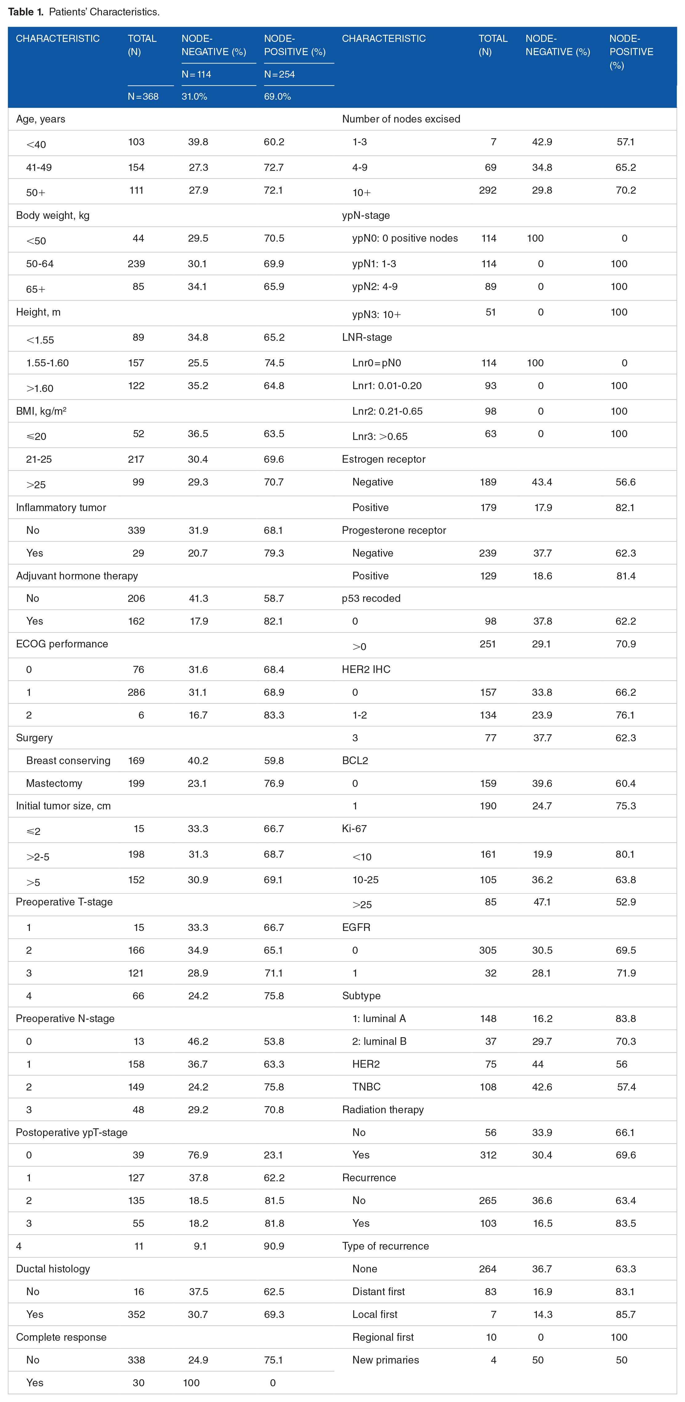
Figure 1’s top panel shows the unadjusted DFS according to ypN or according to LNRc. ypN was highly significant with a log-rank P-value of 1.93 × 10⁻⁶, and LNRc more so, with a log-rank P-value of 4.66 × 10⁻¹¹, that is, 41000 times more significant than ypN. LNRc identified a low-risk node-positive group (Lnr1, blue curve) with DFS comparable to node-negative patients, and a high-risk node-positive group with much shorter survival (Lnr3, red curve). Gini’s mean difference of the RMST’s at a time horizon of 72 months showed a wider average prognostic separation of 14.0 months (95% CI: 10.1-18.1) between pairs of LNRc categories, as compared with 11.9 months (CI: 7.4-16.9) between pairs of ypN categories, 1-sided bootstrap P = .241.

Figure 1.

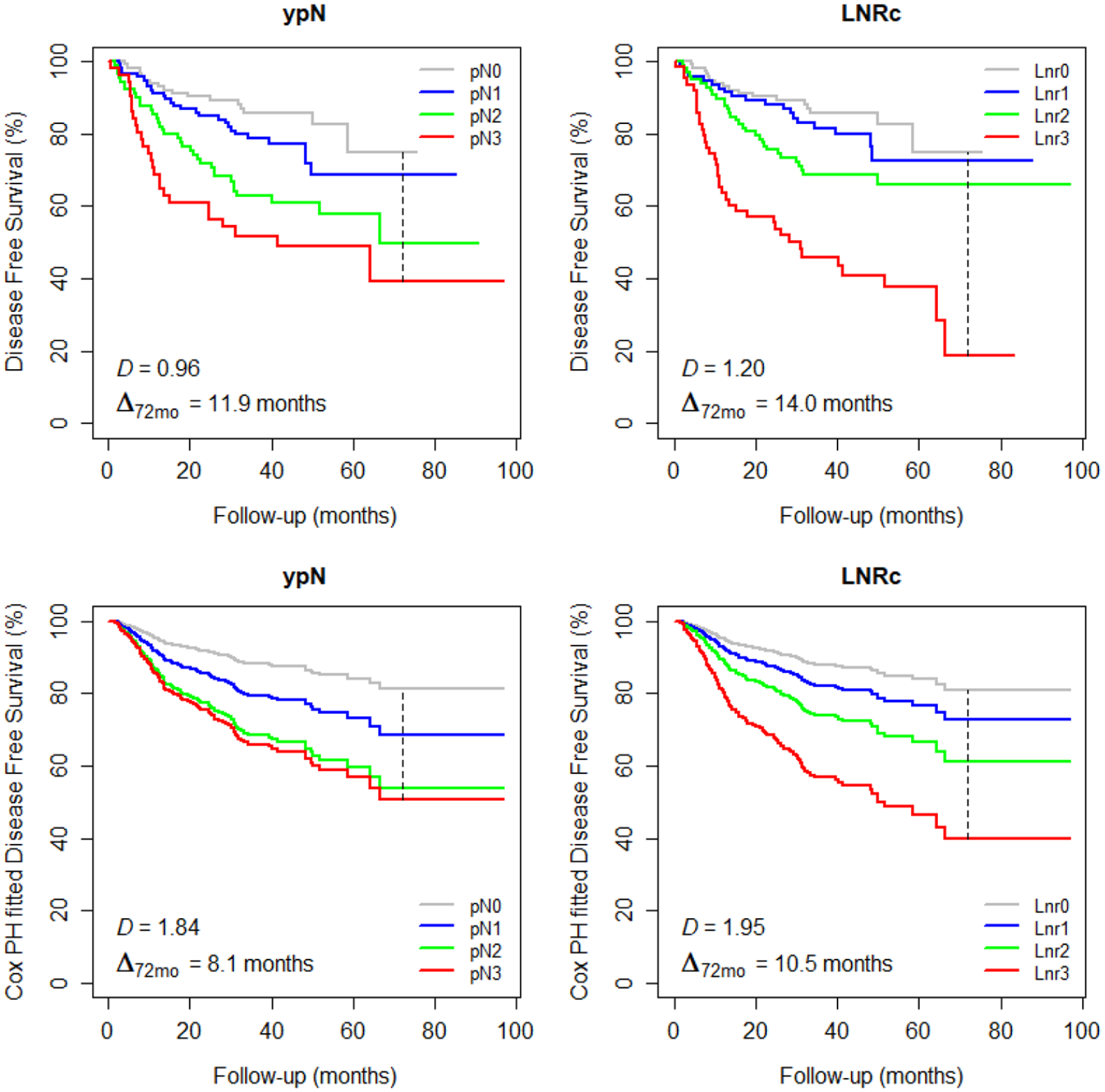
Disease free survival (DFS) according to ypN or LNRc classification. Top, unadjusted DFS; bottom, Cox-adjusted DFS. Vertical dash line, time horizon. D, Royston-Sauerbrei’s measure of prognostic separation. Δ_72mo, Gini’s mean difference of restricted mean survival times, at 72 months horizon.

Table 2 lists the variables that were selected as the most important confounders for DFS according to the AIC. The model shows that ypT stage, positive EGFR, preoperative N stage, Ki-67, inflammatory primary tumor, and progesterone receptor status were predictors of increased risk of event (shorter DFS), whereas radiation therapy and hormone therapy were significantly associated with reduced risk of event (longer DFS).

Table 2.

Confounder Model for Disease Free Survival.

Characteristic	Modeling	Hazard ratio, 95% CI	Stability (% selected)
ypT stage*	Continuous	1.94 (1.58-2.39)	100.0
Radiation therapy	Binary	0.43 (0.26-0.71)	93.5
Adjuvant hormone therapy	Binary	0.51 (0.31-0.86)	90.8
Ki-67*	Continuous	1.01 (1.01-1.02)	90.2
Preoperative N-stage	Continuous	1.44 (1.11-1.88)	89.8
EGFR*	Binary	2.11 (1.20-3.74)	79.4
Tumor inflammatory	Binary	2.07 (1.14-3.74)	77.9
Progesterone receptor	Binary	0.66 (0.38-1.16)	52.0

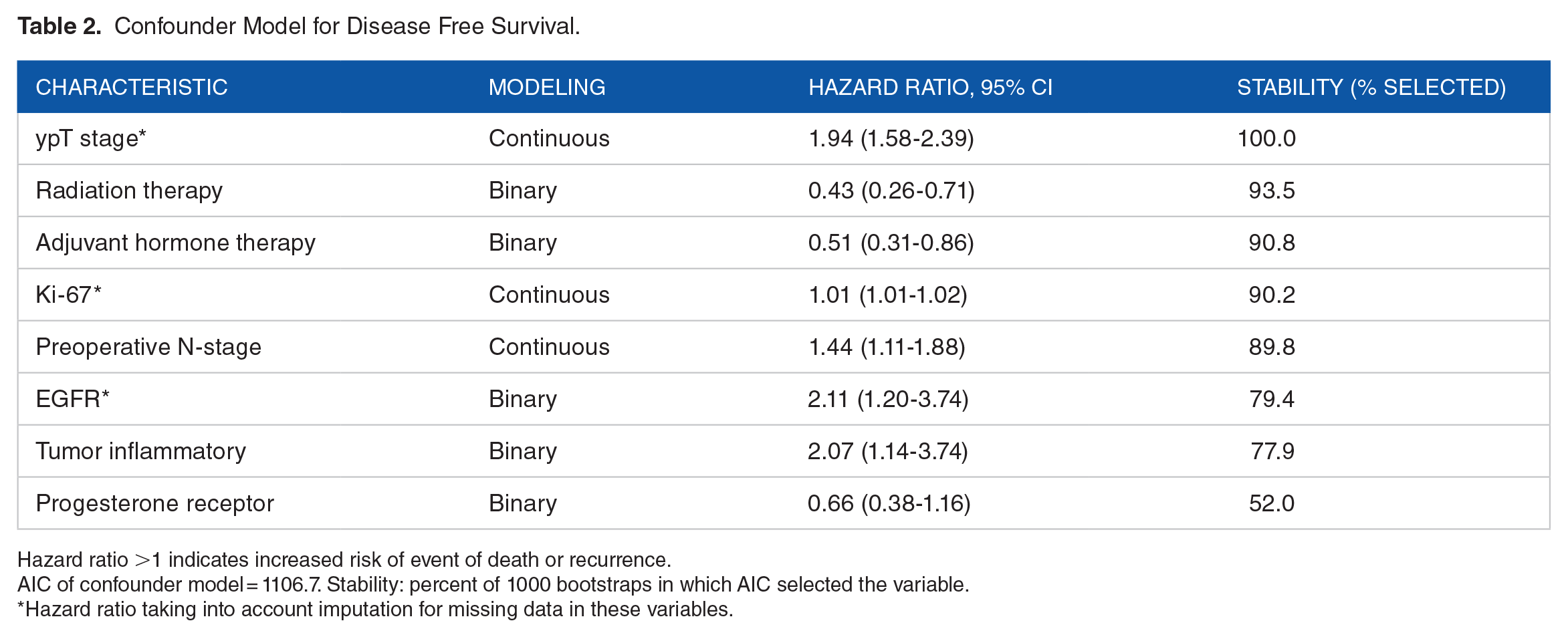
Hazard ratio >1 indicates increased risk of event of death or recurrence.

AIC of confounder model = 1106.7. Stability: percent of 1000 bootstraps in which AIC selected the variable.

Hazard ratio taking into account imputation for missing data in these variables.

Figure 1’s bottom panel shows the adjusted DFS according to ypN or LNRc. Adjusted DFS were modeled by adding ypN or LNRc to Table 2’s confounder model. The fitted survivals resulted in Gini’s mean difference for ypN of 8.1 months (CI: 5.9-10.5), versus LNRc 10.5 months (CI: 8.4-12.8), 1-sided bootstrap P = .066.

Table 3 summarizes the ypN and LNRc survival model metrics. The crude (unadjusted) RMSTs correlated with the ypN levels, declining from 62.4 months to 41.4 months with ypN0-ypN3. Gini’s mean difference was 11.9 months, already mentioned in Figure 1. The adjusted RMSTs also correlated with ypN, although ypN2 did not separate well from ypN3, RMST 52.0 versus 50.4 months. LNRc related more closely with crude and adjusted RMSTs, declining from 62.4 to 36.3 months (crude RMSTs) and from 64.3 to 44.9 months (adjusted RMSTs) with Lnr0 to Lnr3. The hazard ratios of the LNRc categories within the confounder model showed good balance, from the reference hazard ratio 1.00 for Lnr0 to 4.39 for Lnr3. Note that Gini’s mean differences Δ_72months of the adjusted RMSTs were narrower than the unadjusted Δ_72months, reflecting an effect of the confounder model contributing to prognosis. Nevertheless, the separation by LNRc remained wider than ypN, 10.5 versus 8.1 months.

Table 3.

Survival and Model Metrics Comparing ypN With LNRc.

	Metric	CM	ypN				LNRc
Univariate	Crude RMST (months)	NA	ypN0	ypN1	ypN2	ypN3	Lnr0	Lnr1	Lnr2	Lnr3
			62.4	57.8	49.3	41.4	62.4	59.6	53.9	36.3
	Δ_72months, Gini’s mean difference of crude RMSTs	NA	11.9 months				14.0 months
Multivariate models	Adjusted RMST (months)	NA	ypN0	ypN1	ypN2	ypN3	Lnr0	Lnr1	Lnr2	Lnr3
			64.4	58.9	52.0	50.4	64.3	60.7	55.5	44.9
	Δ_72months, Gini’s mean difference of adjusted RMSTs	NA	8.1 months				10.5 months
	Node hazard ratios in confounder model	NA	ypN0	ypN1	ypN2	ypN3	Lnr0	Lnr1	Lnr2	Lnr3
			1.00	1.81	2.99	3.30	1.00	1.52	2.34	4.39
	dAIC, change of Akaike information criteria	0	−29.00				−38.41
	R2N, Nagelkerke index of explained variation	0.202	0.249				0.269
	D, Royston-Sauerbrei’s measure	1.543	1.835				1.947
	R2D, Royston-Sauerbrei’s index of separation	0.362	0.446				0.475
	C-index, concordance index	0.724	0.755				0.765
	NRI, net reclassification improvement	NA	0.441				0.605

Abbreviations and notes: Δ_72months, Gini’s mean difference of the RMSTs; for Δ_72months, R2N, D, R2D, C-index and NRI, as defined in the labeled rows above: higher value = better; CM, confounder model (no lymph node variable); dAIC, reduction of AIC compared with confounder model (defined in Table 2): more negative = better; NA, not applicable; RMST, restricted mean survival time at time horizon 72 months.

All indices listed in Table 3, from AIC to NRI, showed that the confounder model with ypN improved markedly over the confounder model without lymph nodes. LNRc further improved over ypN.

Figure 2’s top panel explored among node-positive patients the effect of separating them into subgroups according to their ypN status. LNRc identified significantly different prognoses among the ypN1 and ypN3 patients and approached significance among the ypN2. Gini’s mean difference showed a separation Δ in ypN1 patients of 8.8 months (out of 30 months horizon = 29% of the expected timespan), in ypN2 of 6.4 months (out of 60 months = 11%), and in ypN3 of 17.9 months (out of 60 months = 30%). By contrast, Figure 2’s bottom panel showed that ypN was significant in none of the LNRc subgroups. Among patients classified according to their ypN status, LNRc added prognostic information. Among patients classified according to their LNRc status, ypN did not add to prognostication.

Figure 2.

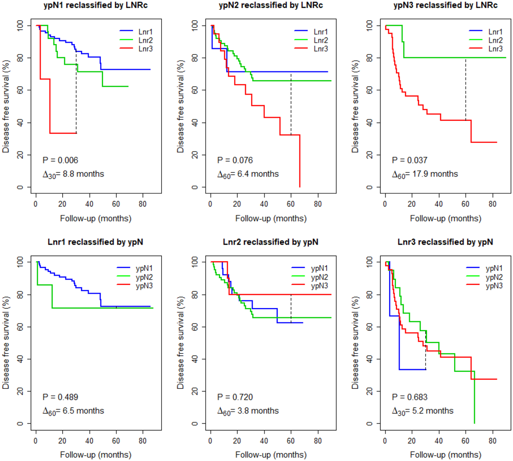
ypN subclassified by LNRc (top), and LNRc subclassified by ypN (bottom).

Discussion

A large body of literature presents the well-known prognostic indices,¹⁵ with extensive discussions of the comparative merits.^21,22 This study contributes to the debate with the rediscovery of a dispersion metric, owing to the renewed interest in RMST. Gini’s mean difference concept is straightforward. It addresses separation intuitively. It facilitates reading the survival results of prognostic markers.

Gini’s mean difference was expressed in months, which sets it aside from unitless metrics. Another divergence from other metrics is the dependence of RMST on the time horizon, or time by which the mean is restricted.⁴ Obviously, the area under the survival curve changes when the horizon changes, which would also affect Gini’s mean difference computed from the RMSTs. We found drawing a vertical line on the survival graphs could unobtrusively yet unmistakably communicate the choice of time horizon. Furthermore, taking care that Δ explicitly subscripted the time horizon could facilitate the evaluation of the results. In Figure 2’s top panel, Δ of 8.8 months among ypN1 patients appears small compared with Δ of 17.9 months among ypN3, until one notices that ypN1 distribution of follow-up imposed a time horizon half ypN3’s time horizon; thus, 8.8 months over 30 months, now reads as far from negligible. Dependence of RMST on the time horizon has been considered a limitation²; instead, we find taking it into account is instructive.

The lymph node hazard ratios (Table 3, middle row) were much larger than any of the other covariates (Table 2); their adjusted Gini’s mean differences were 4-months smaller than the Δ_72months of the unadjusted RMSTs. This suggests that Gini’s mean difference could help against over-optimism to provide a realistic interpretation. Paradoxically, these smaller Δ_72months in multivariate models do not diminish the importance of lymph node involvement. Gini’s mean difference changed from 11.9 to 8.1 months (ypN), or from 14.0 months to 10.5 months (LNRc), in a model including the 8 covariates of Table 2. That implies the lymph node involvement multivariate prognosis weighed twice more than the 4 months attributable to the 8 covariates. Gini’s mean differences convey information that hazard ratios or P-values cannot.

No biomarker has been shown to supersede measures of lymph node involvement in non-metastatic breast cancer. Table 2 represents the best (by AIC) combination of factors without lymph nodes. If the factors were sufficient, adding a lymph node covariate should not have improved the model. To the contrary, as commented above, the number of positive nodes far surpassed the other best combined prognostic factors. That is in line with the AJCC²³ staging which incorporated the number of positive nodes since the first edition, though cutoff categories changed over time. The lymph node ratio improved on the number of positive nodes. Moreover, the lymph node ratio identified different prognostic subgroups among patients classified by ypN, whereas the reverse did not hold, ypN did not uncover significant differences among patients classified by LNRc (Figure 2). These indicate that ypN-classified groups are heterogeneous, the lymph node ratio could be a more robust prognosticator.

This study was a head-to-head comparison of pre-defined classifications. We did not search alternative optimal cutoffs. The relationship between lymph node involvement and mortality is quite linearly monotonous. It has been argued that there are no true biological cutoffs.^24,25 However, determining a pragmatic cut point could be important to adapt therapy, such as deciding on the duration of adjuvant chemotherapy or choosing the type of radiotherapy, to include or not lymph node regions in radiation treatment fields according to the lymph node ratio.^26,27

Should we advocate axillary lymph node dissection after neo-adjuvant chemotherapy? Although most patients presented with advanced local-regional disease, the rate of local-regional recurrence was 4.6% (17 of 368 patients, Table 1). That rate is lower than the 7% locoregional recurrences reported in another study, suggesting that the therapeutic strategy of axillary dissection and radiotherapy was appropriate. However, axillary dissection and radiotherapy incur increased risk of morbidity that we did not assess. Positron emission tomography (PET) can establish the preoperative N-stage. Sequential pre-treatment FDG-PET for breast cancer has been shown to be a predictor of pathologic response.^28,29 Pathologic response, indicated by ypT, and N-stage were strong prognostic factors (Table 2). In a study comparing preoperative FDG-PET with the lymph node ratio, the survival prognostic value of PET came close to that of the lymph node ratio.³⁰ These observations suggest that FDG-PET might be a surrogate prognostic indicator and could help to select the type or the intent of axillary surgery, for disease control, or for diagnostic-prognostic purpose.

Limitations of the study include the relatively small sample size which did not allow detailed subgroup analyses. Models were not established in advance. FDG-PET was done in few patients and was reported separately.

Strengths include the prospective design with MR imaging. The population of patients and the treatment management were homogeneous. Analyses were done without data dredging, reducing the risk of retrospective bias. Application of Gini’s mean difference is innovative, opening new perspectives in clinical exploration.

Conclusion

Gini’s mean difference of RMSTs is shown to be applicable in an observational study of prognostic factors composed of more than 2 levels. Lymph node involvement was the foremost predictor of survival, with a predicting weight twice that of other markers. A nodal ratio-based classification outperformed a number-based classification. At a follow-up time horizon of 72 months in a multivariate model, the lymph node ratio predicted a survival time difference by 2.4 months wider than that predicted by the number of positive nodes.

Footnotes

Funding:

The author(s) received no financial support for the research, authorship, and/or publication of this article.

Declaration of conflicting interests:

The author(s) declared no potential conflicts of interest with respect to the research, authorship, and/or publication of this article.

Author Contributions

Study concept, BK, VVH. Initial draft, BK, VVH. Data collection, BK, SAI. Data analyses, BK, OG, VVH, SAI. Software design, OG, VVH. Writing and final approval, BK, OG, VVH, SAI.

Ethics Approval

The study protocol had been reviewed and approved by the institutional review board at the Seoul National University Hospital.

Consent to Participate

Informed consent was obtained from all patients.

Consent for Publication

Not applicable, no identifying information were collected.

ORCID iD

Vincent Vinh-Hung

Availability of Data and Material

Data is available at DOI: 10.21227/mg5y-7c64 or on request by email to first author: bhumsuk@snu.ac.kr

Code Availability

Code is available at DOI: 10.17632/sfvtmrd8z9.1 and at temporary link

References

Trinquart

Bill-Axelson

Rider

. Restricted mean survival times to improve communication of evidence from cancer randomized trials and observational studies. Eur Urol. 2019;76:137-139.

Kloecker

Davies

Khunti

Zaccardi

. Uses and limitations of the restricted mean survival time: illustrative examples from cardiovascular outcomes and mortality trials in type 2 diabetes. Ann Intern Med. 2020;172:541-552.

Ben-Aharon

Magnezi

Leshno

Goldstein

. Median survival or mean survival: which measure is the most appropriate for patients, physicians, and policymakers? Oncologist. 2019;24:1469-1478.

Royston

Parmar

. Restricted mean survival time: an alternative to the hazard ratio for the design and analysis of randomized trials with a time-to-event outcome. BMC Med Res Methodol. 2013;13:152.

Perrin

, et al. Is there a utility of [18F]FDG-PET before surgery in breast cancer? A 15-years overall survival analysis. World J Clin Oncol. 2021 (in press).

Vinh-Hung

Bourgain

Vlastos

, et al. Prognostic value of histopathology and trends in cervical cancer: a SEER population study. BMC Cancer. 2007;7:164.

Gini

. Variabilità e Mutabilità. Contributo allo Studio delle Distribuzioni e delle Relazioni Statistiche. Tipografia di Paolo Cuppini; 1912.

Keam

Kim

, et al. Clinical significance of axillary nodal ratio in stage II/III breast cancer treated with neoadjuvant chemotherapy. Breast Cancer Res Treat. 2009;116:153-160.

Keam

Park

, et al. Nomogram predicting clinical outcomes in breast cancer patients treated with neoadjuvant chemotherapy. J Cancer Res Clin Oncol. 2011;137:1301-1308.

10.

Recht

Edge

Solin

, et al. Postmastectomy radiotherapy: clinical practice guidelines of the American Society of Clinical Oncology. J Clin Oncol. 2001;19:1539-1569.

11.

Peto

Pike

Armitage

, et al. Design and analysis of randomized clinical trials requiring prolonged observation of each patient. II. analysis and examples. Br J Cancer. 1977;35:1-39.

12.

Sauerbrei

Royston

. A new strategy for meta-analysis of continuous covariates in observational studies. Stat Med. 2011;30:3341-3360.

13.

Van Buuren

. Multiple imputation of discrete and continuous data by fully conditional specification. Stat Methods Med Res. 2007;16:219-242.

14.

Sauerbrei

Royston

. Building multivariable prognostic and diagnostic models: transformation of the predictors by using fractional polynomials. J R Stat Soc A Stat Soc. 1999;162:71-94.

15.

Steyerberg

Pencina

Lingsma

Kattan

Vickers

Van Calster

. Assessing the incremental value of diagnostic and prognostic markers: a review and illustration. Eur J Clin Invest. 2012;42:216-228.

16.

Royston

Sauerbrei

. A new measure of prognostic separation in survival data. Stat Med. 2004;23:723-748.

17.

Harrell

Jr . Regression Modeling Strategies With Applications to Survival Analysis and Logistic Regression. University of Virginia; 2000:484-485.

18.

Jurecková

Picek

. Robust Statistical Methods With R. Chapman & Hall/CRC; 2006.

19.

Glasser

. Variance formulas for the mean difference and coefficient of concentration. J Am Stat Assoc. 1962;57:648-654.

20.

Keam

Kim

, et al. Prognostic impact of clinicopathologic parameters in stage II/III breast cancer treated with neoadjuvant docetaxel and doxorubicin chemotherapy: paradoxical features of the triple negative breast cancer. BMC Cancer. 2007;7:203.

21.

Choodari-Oskooei

Royston

Parmar

. A simulation study of predictive ability measures in a survival model I: explained variation measures. Stat Med. 2012;31:2627-2643.

22.

Austin

Pencinca

Steyerberg

. Predictive accuracy of novel risk factors and markers: a simulation study of the sensitivity of different performance measures for the Cox proportional hazards regression model. Stat Methods Med Res. 2017;26:1053-1077.

23.

American Joint Committee for Cancer. American Joint Committee for Cancer Staging and End-Results Reporting. Manual for Staging of Cancer 1977. American Joint Committee; 1977.

24.

Vinh-Hung

Storme

. No nodal cutoff in node-positive breast cancer women treated with mastectomy. Breast Cancer Res Treat. 2006;98:173-178.

25.

Vinh-Hung

Leduc

Baudin

, et al. Axillary lymph node involvement in breast cancer: a random walk model of tumor burden. Cureus. 2019;11:e6249.

26.

Tai

Joseph

Sadikov

Mahmood

Lien

. Nodal ratios in node-positive breast cancer—long-term study to clarify discrepancy of role of supraclavicular and axillary regional radiotherapy. Int J Radiat Oncol Biol Phys. 2007;68:662-666.

27.

Kim

Park

Kim

, et al. Clinical significance of lymph-node ratio in determining supraclavicular lymph-node radiation therapy in pN1 breast cancer patients who received breast-conserving treatment (KROG 14-18): a multicenter study. Cancers (Basel). 2019;11:680.

28.

Keam

Koh

, et al. Early metabolic response using FDG PET/CT and molecular phenotypes of breast cancer treated with neoadjuvant chemotherapy. BMC Cancer. 2011;11:452.

29.

Keam

Koh

, et al. Predictive value of FDG PET/CT for pathologic axillary node involvement after neoadjuvant chemotherapy. Breast Cancer. 2013;20:167-173.

30.

Vinh-Hung

Everaert

Gorobets

, et al. Breast cancer preoperative (18)FDG-PET, overall survival prognostic separation compared with the lymph node ratio. Breast Cancer. 2021;28:956-968.

Lymph Node Ratio after Neoadjuvant Chemotherapy for Stage II/III Breast Cancer: Prognostic Value Measured with Gini’s Mean Difference of Restricted Mean Survival Times

Abstract

Keywords

Introduction

Methods

Patients

Survival analyses

Confounder model

Prognostic indices

Gini’s mean difference

Software

Results

Discussion

Conclusion

Footnotes

Funding:

Declaration of conflicting interests:

Author Contributions

Ethics Approval

Consent to Participate

Consent for Publication

ORCID iD

Availability of Data and Material

Code Availability

References