Sage Journals: Discover world-class research

Abstract

Time is one crucial dimension conveying information in animal communication. Evolution has shaped animals’ nervous systems to produce signals with temporal properties fitting their socio-ecological niches. Many quantitative models of mechanisms underlying rhythmic behaviour exist, spanning insects, crustaceans, birds, amphibians, and mammals. However, these computational and mathematical models are often presented in isolation. Here, we provide an overview of the main mathematical models employed in the study of animal rhythmic communication among conspecifics. After presenting basic definitions and mathematical formalisms, we discuss each individual model. These computational models are then compared using simulated data to uncover similarities and key differences in the underlying mechanisms found across species. Our review of the empirical literature is admittedly limited. We stress the need of using comparative computer simulations – both before and after animal experiments – to better understand animal timing in interaction. We hope this article will serve as a potential first step towards a common computational framework to describe temporal interactions in animals, including humans.

Keywords

zoology evolutionary biology evolutionary neuroscience agent-based modelling bioacoustics rhythm chorusing turn-taking

Introduction

Communication is a key component in the lives of biological organisms and can occur through several channels, including acoustics, bioluminescence, and movement displays. Animals communicate to attract mates, to maintain relationships with one or more individuals, and to defend territories or resources.^1,2 Many animal species have been observed signalling over long distances to communicate with conspecifics. Attenuation and degradation of signals impose limits on communication.³ To ensure an effective transfer of information, the signal must be transmitted rapidly and accurately from the source to the receiver. The receiver must be capable of detecting the signal, discriminating the relevant characteristics that structure a signal and locating its origin.^3,4 For effective communication to be established, one may try to avoid overlap during signalling⁵ (although overlap is not necessarily a negative feature of a communication system). However, signals that overlap in 1 dimension need not overlap in another. In animal communication, a dimension can be defined as a physical and perceptual characteristic, such as fundamental frequency or peak amplitude. Two signals that overlap in time can be produced at different fundamental frequencies and might still be discriminated by the receiver. For the purpose of this article, signal overlap will be considered as the case where signals partly (or fully) occur at the same time.

Over the last few decades, the field of animal communication has seen an increasing focus on the temporal dimension of signals. In many species, rhythm, here defined as the temporal (possibly repeated) structure of signals, carries essential information for communication between individuals.^6–8 Physiologists have long been interested in the behavioural periodicity found in species across the animal kingdom. Examples of biological rhythmic activity include the beating of the heart, respiration, and locomotion.^9,10 Focussing on a millisecond-second timescale, we find rhythmic signalling, which also relies on different neural circuitry from rhythms at the level of interacting cells. Some fascinating examples of interactive rhythms include the individual timing behaviours exhibited by animals living in aggregated communities which can result in striking natural phenomena such as the synchronous flashing of fireflies, and cricket choruses at dusk and dawn.^11–13 Similar forms of collective behaviours can be achieved through different mechanisms, and similar mechanisms can produce very different forms of collective behaviours.

At present, only a handful of computational models of animal rhythmic behaviours have been developed to provide a better understanding of the mechanisms behind group timed signalling.^13–15 Most of the research in the literature has focused on modelling the communication systems of amphibians, insects, crustaceans, and some bird species.^{11,12,16–19} Models are, in a way, quantitative hypotheses that can be employed to test and predict interactive dynamics of rhythms in communication. Modelling is useful to test the internal consistency of these hypotheses and explore the hypotheses’ space before any experiment is run. Models also serve to call attention to mechanisms that would otherwise not have been recognized and can be used to compare predictions with observations of natural data. Quantitative formulations of a problem help scientists to be more rigorous and better consider the details of a system composed of interacting parts. Most importantly, modelling is the necessary counterpart of empirical work: empirical findings should be summarised via mathematical/computational models, which can be used to advance new hypotheses that are then empirically tested. Finally, good models can become standardised and serve as potential tools for cross-species comparisons. Still little is known about rhythmic communication in mammals, and, apart from humans, their rhythmic signalling is rarely modelled.

In this article, we provide an overview of several existing models that have been used in the study of animal rhythmic communication, including human speech and music. We first discuss some basic concepts of dynamical systems and the mathematics of timing. We then present a real-life example of each individual model along with the computational model resulting from simulated data. To uncover the key similarities and differences in the underlying mechanisms behind each observed example, the mathematical models are then compared. The purpose of this article is 2-fold. It is a first step towards a common computational framework to describe temporal interactions in animals.^20–22 More importantly, it represents an open letter to the scientific community performing animal empirical work, stressing the need for using computer simulations to better understand animal timing in interaction.

From Oscillators to Models of Rhythm

The rhythms produced by species involved in long-distance signalling appear to be under the control of central nervous oscillators.^9,13,20 Central nervous oscillations are the rhythmic patterns of neural activity found in the central nervous system. An oscillator is any system that executes periodic behaviours that fluctuate between 2 extremes, which can be illustrated using a characteristic sinusoidal waveform.²³ Every oscillator has its own specific endogenous rhythm. Oscillator dynamics can be visualised by plotting their motion through a phase space. A phase space is a visual representation of a dynamical system in which each point corresponds to 1 possible state over time.^24,25 In acoustic communication, this phase space can be used to visualise the time interval between onsets of adjacent signals as a function of time.

The emerging patterns from the collective interactions between neighbouring individuals emerge from precisely timed phase relationships. Here, phase relationships refer to the fraction of the oscillator cycle that has elapsed relative to the origin of the signal. These marked interactions can take the form of phase advances, phase delays, or changes in the endogenous rhythms of the oscillators of each individual.²⁰ Stable-limit cycle oscillators are systems that, when perturbed by the signal of a neighbour, have their endogenous rhythm advanced or delayed, but eventually return to their original free-running period.^10,23 These concepts, originally developed in physics and physiology, have been incorporated in different models of animal rhythms (see Supplemental Material and Table 1).

Table 1.

Definitions of key concepts in animal rhythmic communication.

Alternation	The timing relationship between 2 signals whose phase relationship is 180°.
Antisynchrony	The timing relationship between 1, 2, …, N signals whose phase relationship is 360°/k, where k = 1, 2, …, N. Alternation is a special case of antisynchrony, namely, when N = k = 2.
Effector	A system that acts in response to a signal.
Focal Animal	Individual whose behaviour is observed.
Inter-onset interval	Time interval between the onsets of 2 adjacent calls.
Isochronous	Series of events separated by a constant time interval. It is characteristic of 1 signal.
Lag (neural)	Duration of neuronal signal transmission and consequent activation of an effector in response to that signal.
Neighbour	Individual that affects the signal timing of the focal.
Phase change/shift	Variation in the difference between the time of focal response relative to the signal of its neighbour, which can take the form of either an increase (relative advance) or decrease (relative delay).
Rhythm	The temporal structure of signal events, possibly including repetition of temporal patterns. Musical rhythm is only loosely related to rhythm in animal signals, as the former entails cognitive concepts such as beat, tactus, and metre.
Signal sequence	Train of signal units.
Synchronous	Series of individual events co-occurring at the same time. The relationship of synchrony can hold between 2, or among multiple, signals.

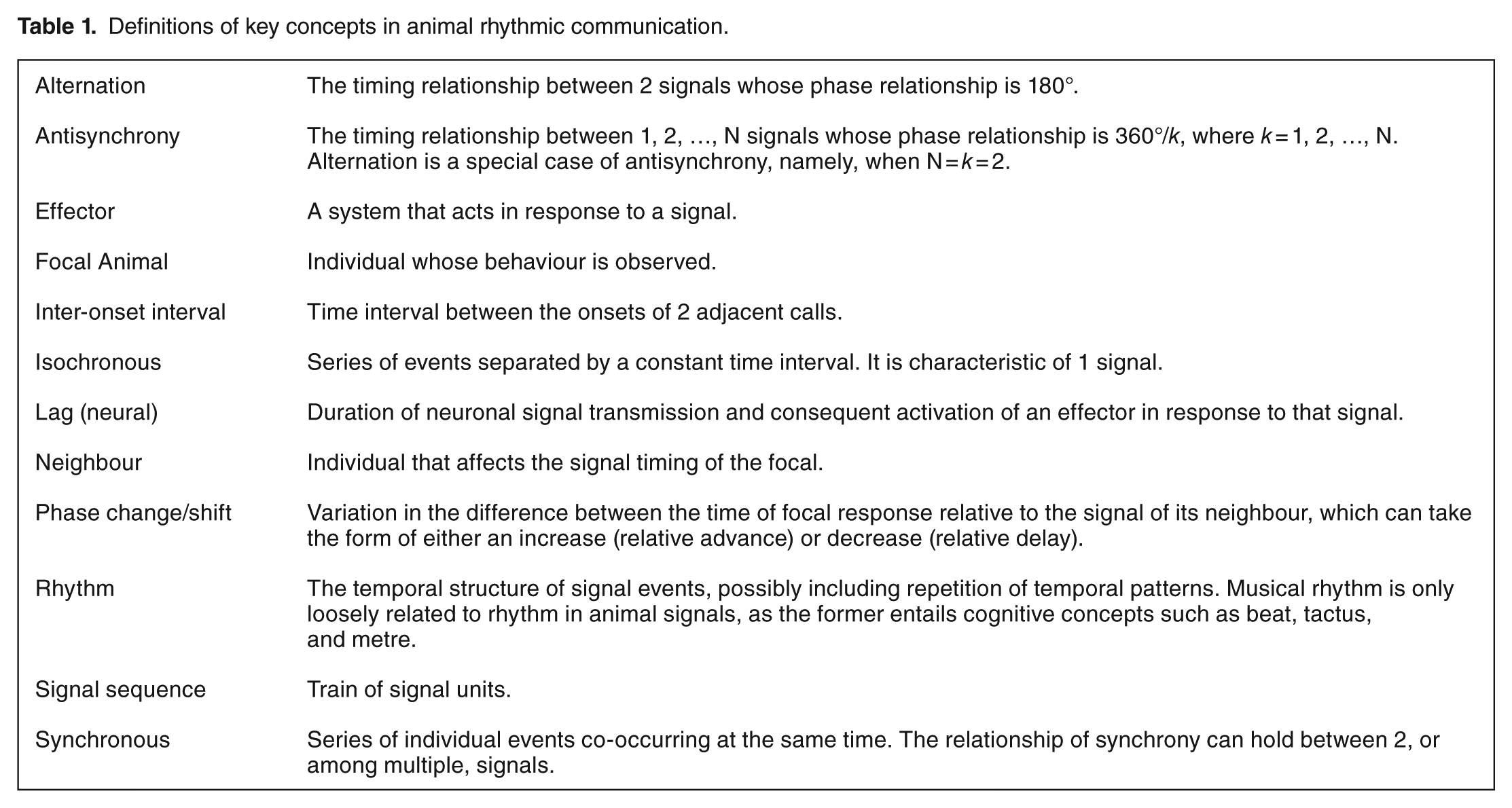
In large communities, each individual has its own free-running rhythm, but this can be adjusted in response to the signals of nearby neighbours. Individuals from signalling species have precise timing abilities and often signal with specific phase relationships or lags (ie, delays) in response to the signals of conspecifics. The 2 best-known aggregate timing phenomena are synchrony and alternation, but combinations of the 2 have also been documented in nature.²⁰ In addition, synchrony and alternation are not always clear-cut: the signals of chorusing individuals may only partially overlap and alternating signalling can sometimes lead to short periods of synchrony. These observations are consistent across species using acoustic or bioluminescent communication channels.²⁰

Here, we define synchrony as the precise temporal co-occurrence of signals with an external rhythmic signal, so that signal and external signal have a phase angle close to 0°. Alternation is a form of non-synchronous coordination, with no overlap between the calling individuals and a relative phase angle of 180°.²⁶

Oscillators can be coupled to the signals of nearby neighbours. The most familiar mode of organisation of these oscillators is synchrony. In 1665, the clockmaker Christiaan Huygens noticed that if he hung 2 pendulum clocks side by side on the wall and desynchronised them, the pendulums would eventually swing in perfect synchrony.²⁷ He theorised that the clocks were reciprocally influenced by tiny vibrations in their common support. This pulse coupling turns out to be common in biological systems, but modelling this coupling requires modelling nonlinearities.^23,28 For the case of animal rhythmic communication, nonlinear behaviours mean that the temporal properties of an individual signalling are not a linear function of the temporal properties of a conspecific.

Fireflies are a good example of a ‘pulse coupled’ oscillator system as their rhythmic interactive behaviour is triggered only when one individual perceives the sudden flash of its neighbour and shifts its rhythm accordingly. Male winged beetles of the order Coleoptera, commonly known as fireflies, gather in trees during twilight. They conspicuously use bioluminescence to attract mates. Initially, their flickering is uncoordinated, but as the night deepens, their signals start coupling and they pulsate in synchronous flashes.^11,12 Although some animal examples such as the flashing of fireflies approximate synchrony, idealized perfect synchrony never occurs in real populations. This is due to the large amounts of variation observed in nature, which results in different distributions of individual timing abilities found across species.^29–31

Mechanisms of Individual Timing in Groups

As individual mechanisms for rhythmic inter-individual interactions do not exist in a vacuum, one must study how species adjust their timing with respect to the timed behaviour of nearby neighbours.

The existing literature in animal interactive timing can be classified into categories based on the relationship between the signaller and the receiver.⁵ A chorus is the interactive signalling between 2 or more individuals and often involves males, as observed in katydids.¹³ Duets, often occurring in songbirds and insects,^19,32 are a special subset of choruses as they involve only 2 individuals. Duetting can occur in male-female pairs (though see Snow³³). Given the comparative aim of this article, as modelling choruses becomes increasingly complex with each additional individual, only models of duets will be presented.

Precise temporal interactions can be discerned despite high signalling rates found in nature. Due to natural variations within and between individuals, species may need to adjust their timing relative to their neighbours to increase their reproductive fitness. Species can adjust their timing using 2 classes of mechanisms.³⁴ Species exhibiting homoepisodic mechanisms detect the signal of their neighbour and respond nearly immediately by producing their own signal. In anurans, some species partially overlap their calls in this manner based on the stimuli produced by surrounding conspecifics.¹⁷ The homoepisodic timing adjustment is thus mainly responsible for synchronous onsets in collective rhythmic signalling. However, it cannot explain all synchronous interactions as the time interval between signals from adjacent neighbours is often shorter than the effector delay and sometimes even shorter than the time it takes for the signal to travel from one individual to the next. Proepisodic mechanisms are those where the focal individual’s signal is produced based on the previous signal(s) of the neighbour. For instance, proepisodic timing has been observed in humans playing music³⁵ and some other non-human animals.^26,36,37 Two types of proepisodic mechanisms have been identified in the field of animal rhythms: perfect synchrony and phase-delay synchrony. Due to the mostly non-human focus of this article, we refer to timing mechanisms using homoepisodic or proepisodic,^20,34 as opposed to the loosely related distinction between reactive and predictive mechanisms, more common in cognitive psychology.

Another dichotomy, coming from the human cognitive neuroscience literature, concerns the models of rhythmic behaviour, which can be explicit or implicit.²⁶ Explicit models assume monitoring of signal lengths of discrete temporal units and comparison of preceding lengths to the average of those stored in memory.^38,39 Instead, implicit timing models propose that timing abilities are dependent on neural oscillations, which are coupled to external signals.⁴⁰

Behavioural responses to conspecific or experimentally generated stimuli can be used to infer whether an organism’s timing mechanism is proepisodic or homoepisodic. In the next sections, we will describe different models of animal rhythms and discuss the underlying mechanisms using mathematical and computational tools. For a comparison of some of these models with experimental animal data see Greenfield and Roizen13 and supplement in Ravignani.⁴¹

Formal Description of Alternative Timing Mechanisms

Individual rhythmic behaviours in inter-individual interactions can be summarised as functions of the signalling period of the focal animal $T_{i}$ and the neighbour animal ${T^{'}}_{i}$ at time period $i$ ; the focal animal free-running period $T$ ; the Uniform and Gaussian distributions $U a n d N$ , respectively; and scaling parameters $a, b, c, a n d k$ .

Based on the models described below, we ran computer simulations. Simulations of each mechanism consisted of 2 agents. A neighbour individual would produce a series of signals, either isochronously or with a constant drift, without paying attention to the other individual. The other, focal individual would react to the partner’s signal by adopting one of the modelled mechanisms. Note that, in the simulations below, the signal length equalled 0 for the sake of simplicity. In addition, we posed the constraint that the focal individuals only produced 100 signals in each simulation. (These particular 100 signals eliciting a response where randomly and uniformly sampled.) In the isochronous condition, neighbours’ inter-onset intervals (IOIs) were sampled from a normal distribution with mean 1500 ms and standard deviation 150 ms. In the constant-drift condition, partners’ IOI went from 1000 to 2000 ms in successive steps of 5 ms.

For these simulations, the scaling parameters were: $a = 1 / 2, b = 1 / 10, c = 1 / 5, k = 4$ . The free-running period of the simulated focal animal $T$ was arbitrarily chosen to equal 1500 ms.

Visualizing Simulated Data

Delay-period plots can be used to visualise when a focal individual will signal as a function of the time between the previous 2 signals of a conspecific. The x-coordinate of a point denotes the neighbour’s previous IOI. The y-coordinate of a point denotes the delay, the time elapsed between the last signal of a neighbour and the signal of the focal animal ( $φ_{i}$ in the equations below). Although these scatterplots are similar to phase response curves, the crucial difference is that delay-period plots show absolute, rather than relative, durations. Phase response curves are appropriate in all cases where a free-running period exists. However, as our examples include cases of non-periodicity, we prefer using the delay-period plots. Delay-period plots can be interpreted biologically in different ways. Their main purpose is to represent temporal interactions at the level of single events (the dots) between an animal signalling rate (x-coordinate) and the time passed between an animal signal and a conspecific signal. In this graph, the dots forming a clear linear relationship may represent an individual delay in signalling proportional to the signalling rate of a conspecific.

Rose plots are a visualisation technique similar to histograms. However, although histograms can potentially span any pair of arbitrary values (to include the maximum and minimum of the distribution), rose plots are circular, spanning 0° to 360° (equivalent to 0°). Area segments of a circle are used to convey the frequency distributions of phase angles in a particular phase angle bin. In rose plots, the bin size is usually constant and equal to 360° divided by the number of bins. Keeping the bins constant across rose plots is used to easily compare angular distributions. Here, rose plots show the frequency distribution of the focal (relative) phase, ie, the focal delay divided by the neighbour’s previous period. Rose plots can also have a number of biological interpretations. Their most straightforward interpretation is when an animal will signal if we treat a conspecific as a ‘metronome’. In other words, the points in time at which an animal signals are segmented and grouped relative to (ie, modulo) a conspecific call.

Baseline: The Arousal Model

The most basic model that can be described in the study of animal timing consists of the signals produced by an individual in the absence of a neighbour. An animal that is not influenced by the signals of its neighbour does not show a phase delay or phase advance with respect to a signal because that signal is absent. An individual, alone, will either not signal at all, or time its signals according to its endogenous or free-running rhythm. This is expected to be species-specific and show little variation across individuals of the same species.

Instead of the no-neighbour model, an ‘arousal model’ can be employed for baseline: the focal individual acts due to a simple arousal mechanism, the higher the number of a neighbour’s signals perceived, the higher the number of signals produced, with no temporal relation between these two. To our knowledge, the arousal model has never been used in empirical research; however, an intuitive example could be the timing of contagious barking of dogs.

The delay of the focal animal relative to its partner, $φ_{i}$ , in the arousal model equals⁴¹

φ_{i} = U (0, {T^{'}}_{i - 1})

(1)

In other words, the focal individual signals at a time that is randomly and uniformly sampled from the duration of the previous period of the neighbour. So, as the neighbour increases its period, the focal will be more likely to signal. The simulated data for this model are plotted as delay-period scatterplots (Figure 1) and rose plots (Figure 2). Notice that no particular pattern emerges, as this model constitutes a baseline with no particular time adjustments.

Figure 1.

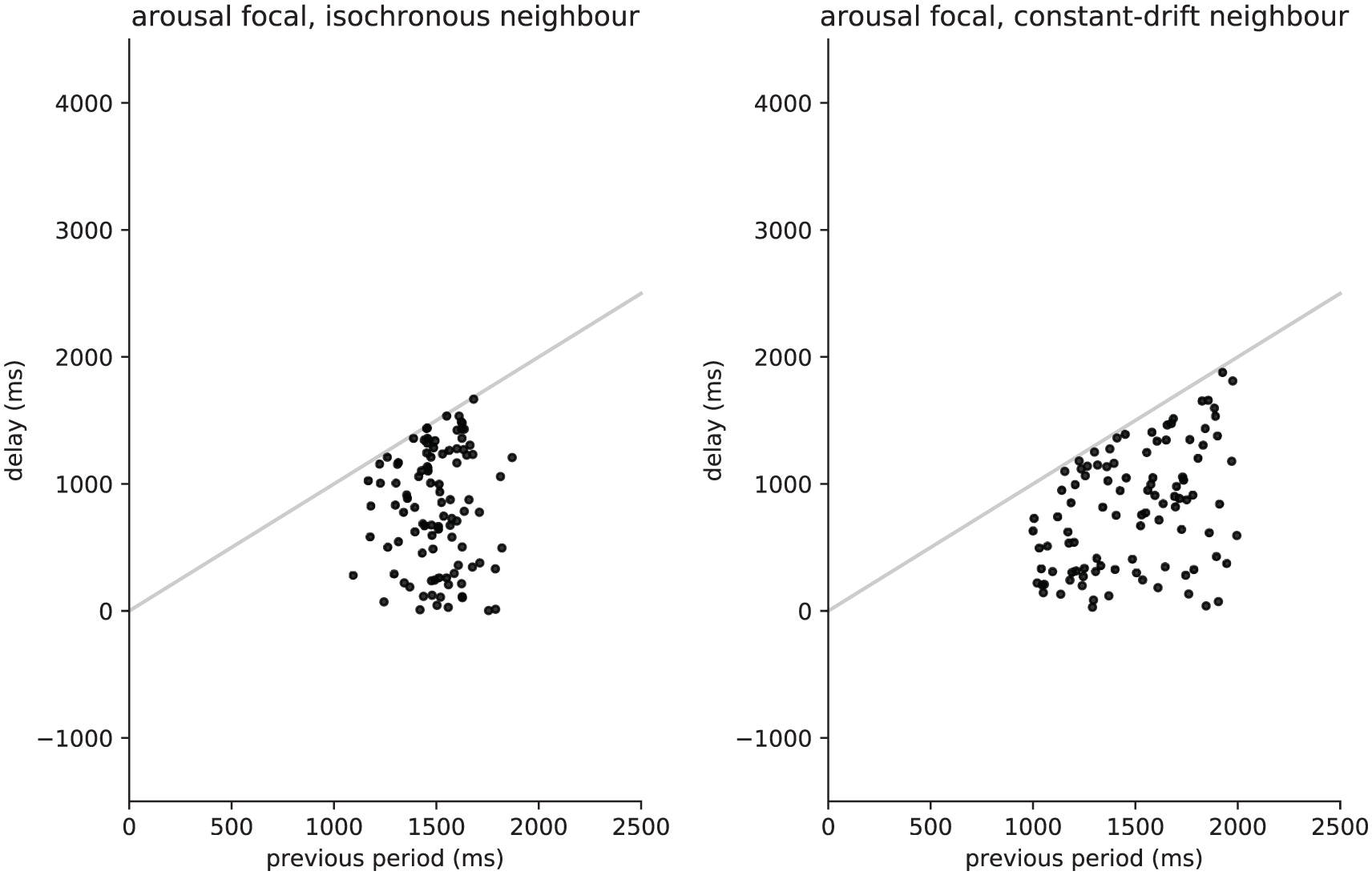
Arousal model plotted using simulated data, showing lag-period plots for a simulated isochronous neighbour (left) and a constant-drift neighbour (right). In these graphs, the focal lag/delay (vertical) is plotted against the partner previous period (horizontal).

Figure 2.

Rose plots of the arousal model showing frequency distributions of relative phases, relative to a simulated isochronous neighbour (left) and a constant-drift neighbour (right).

Self-synchronization and Neural Oscillators

In 1975, Peskin⁴² proposed a model of self-synchronisation using the heart’s natural pacemaker, a cluster of 10 000 cells known as the sinoatrial node. He modelled the cardiac pacemaker as a large number of oscillators all coupled equally strongly to one another and all exhibiting the same dynamic. Each oscillator affects its neighbours only when it fires and can cause nearby oscillators to exceed their firing threshold, in a mechanism commonly known as the integrate-and-fire dynamic. This model shows that the whole system will eventually become synchronised. The mathematical proof comes from the notion of ‘absorption’, ie, the idea that if an oscillator causes another nearby oscillator to cross its threshold, both oscillators will remain in synchrony.^43,44 Strong assumptions were made in this model as all oscillators have identical dynamics. Moreover, synchronisation is more readily observed with increased coupling strength. However, weak oscillator coupling can still lead to synchronisation if the observed frequencies are close to one another.⁴³ Perpetual disorganisation in a system could occur if the oscillators behaved in a discontinuous fashion, and this would never result in synchronous behaviour.^43,44 Alternatively, a system may break off into frequency-locked clusters because of weak coupling between clusters. Local synchrony would arise, and each cluster would fall out of synchrony with neighbouring clusters, yielding global ‘non-synchrony’. Different timing interactions are expected to arise if a model includes a spatial structure that focuses more on local interactions instead of assuming that all oscillators in the model are equally close neighbours. This would lead to some oscillators showing different dynamics. Neurons often behave as coupled oscillators.⁴⁵ It is thus reasonable to expect the dynamics of neurons to resemble those of an oscillator network as described in Peskin’s natural heart pacemaker.^23,44 The rhythms produced are caused by the combined interactions of actions potentials in the central nervous system. Although Peskin’s model is not directly associated with the rhythmic signalling of any species discussed here, its basic underlying ideas are present, to some extent, in most models discussed below.

For instance, related to Peskin’s ideas, the neural oscillator model assumes that the response timing of interacting oscillators depends on the intrinsic rate of a pacemaker in the central nervous system which is triggered by an effector lag, t.²⁰ There is a minimum lag between perception of a signal and the reply that follows. The lag in response of the effector is a measure of the neurophysiological constraints of an organism, specifically its lowest temporal resolution in the perception-action cycle. It describes the velocity of neural transmission and the time it takes for the activation of an effector in response to that signal. Empirical measurements of t indicate values ranging from 50 to 200 ms in insects such as katydids and fireflies.^11,12,34 Rhythms always fluctuate below and above the mean signalling rate as a result of variation in the signal period (T) and the effector lag (t). This model is also known as the saw-tooth oscillator model because the pacemaker ascends periodically from its basal to peak level, hence drawing a saw-tooth with its amplitude over time. Reaching the peak level triggers signal production. If undisturbed, the oscillator has its own endogenous rhythm, which is in principle variable across individuals. Two variations of the neural oscillator model have been adapted to animal signalling: the phase delay (see below) and inhibitory resetting (see Supplemental Material) models.

Phase-Delay Model

Among species that seem to signal in a synchronous manner, 2 mechanisms have been identified: perfect and phase-delay synchronies. As mentioned above, perfect synchrony is hardly achievable in biological systems because of the large amount of variation present in nature. As a consequence, synchrony is detectable as arbitrarily small phase relationships (which would correspond to 1, large frequency bin centred at 0 in Figure 2). From the receiver’s perspective, organisms will identify 2 signals as synchronous if their phase difference is smaller than the organisms’ perceptual timing threshold.

Phase-delay synchrony occurs when an individual delays its signal by an interval equivalent to the delay between its previous signal and a neighbour’s signal (ie, the signal of a neighbour). Male chorusing of neotropical katydids (Neoconocephalus spiza) illustrates this mechanism well.¹⁸ In this interaction, if a neighbour’s signal is presented just before the focal male’s signal, the signal will not be interrupted, but his next signal will be advanced with respect to the previous focal signal onset (see also inhibitory resetting model in Supplemental Material). This means that the first signal was already triggered prior to the signal of the neighbour. This can be explained by a 4-step mechanism where (1) the central nervous system pacemaker ascends slowly from basal to trigger level, (2) the pacemaker descends to basal level after being triggered, (3) external stimuli can instantaneously reset the pacemaker to its basal level, after which (4) the pacemaker resumes its endogenous rhythm. If males signal at similar rates with small fluctuations, the delays will cause rhythms to align within a single period, and synchrony ensues. Even though synchrony and alternation can appear as dissimilar patterns, both phenomena can be achieved using the same phase-delay mechanism.

In its simplest variant, focussing on points (3) and (4) above, the delay of the phase-delay model equals^13,15,20

φ_{i} = N (T, b T)

(2)

In other words, the focal animal signals right after its partner, with a time delay that is randomly and normally distributed around the focal’s free-running period. Notice that this is a simplified version of the model, with effector delay t = 0. Parameter b can be interpreted as the amount of jitter around an isochronous delay: the lower the b, the more isochronous and predictable the signal produced in response to a conspecific.

The simulated data for this model are plotted as delay-period scatterplots (Figure 3) and rose plots (Figure 4). In the delay-period plot (Figure 3), a clear pattern emerges. Data points are concentrated around 1500 ms on both axes. In the isochronous neighbour condition, the focal appears to partly adjust its next onset depending on the neighbour previous period. This is confirmed in the corresponding rose plot (Figure 4, left side), with a high density of data points at or before 0°, equivalent to synchrony. Notice, however, that 1500 ms is in fact the average period of both individuals, which could be a reason for the high density of data points at 0°. The constant-drift neighbour model does not perform as well in terms of its synchronisation precision. The right side of Figure 3 shows that as the period duration varies, the focal’s delay is almost constant. The right side of Figure 4 shows that there is a tendency of the focal to signal within a range of (–90°, +90°) from or to the neighbour, which does not suffice to reach the levels of synchrony seen in the isochronous condition.

Figure 3.

Phase-delay model plotted using simulated data, showing lag-period plots for a simulated isochronous neighbour (left) and a constant-drift neighbour (right). In these graphs, the focal lag/delay (vertical) is plotted against the partner previous period (horizontal).

Figure 4.

Rose plots of the phase-delay model showing frequency distributions of relative phases, relative to a simulated isochronous neighbour (left) and a constant-drift neighbour (right).

Synchrony reached in the isochronous variant of this model can be explained in evolutionary terms. In fact, it is an epiphenomenon of competitive interactions between males: within the group display, males try to jam each other’s signals.¹³ Leaders, whose rhythm is slightly advanced relative to their neighbours, will be more conspicuous, but still contribute to the overall near-synchrony. In many species of Orthoptera, females prefer males that signal before their neighbours in a specific sequence. Sexual selection thus drives males to strive to call in a leader position, as followers have lower reproductive success.³²

Antisynchrony Model

Species that live in large populations with aggregated clusters must process a large quantity of signals and may adjust their signals respectively using a different mechanism. In 1971, Hamilton⁴⁶ proposed the selfish herd theory. This model attempts to explain the spatial behaviour of animals living in aggregated communities. Hamilton’s model predicts that individuals within a population try to reduce predation risk by physically putting other conspecifics between themselves and the predator. The basic assumption of this model is that in aggregations, predation risk is greatest on the periphery and decreases towards the centre. This classical mathematical model for animal behaviour uses the example of frogs living around a circular pond. In this example, frogs are at risk of predation by a water snake and, to minimize this risk, they jump in-between other conspecifics to minimize their ‘domain of danger’.

Recently, however, Hamilton’s model was adapted and applied to animal rhythmic communication,^26,47 and tested in an experiment.⁴¹ Now, instead of each individual varying its location in space as seen in animal spatial aggregations, the caller shifts the ‘temporal location’ of its call onsets within a temporal-acoustic aggregation of conspecifics. In one version of the model, the caller times its vocalisations exactly in the shortest silent space between the calls of the nearby individuals. If all signalling animals try to do so either by delaying their next call or anticipating the next call of a conspecific, the silences between all calls will shorten until eventually their calls will end up in synchrony, or clusters.²⁶ This will lead to a decrease in the conspicuousness of all signallers and lower their predation risk by signalling between the signallers.

The same basic model, when reversed (signal during the longest silences), predicts that call timing will be dynamically shifted to occur at the midpoint or a fraction of the time period between 2 calls of a conspecific.⁴¹ The predicted outcome, in this case, is antisynchrony. Playback experiments with a lone harbour seal (Phoca vitulina) pup showed that the pup timed its calls in an antisynchronous manner. In fact, the seal timed its calls to occur approximately one-quarter of the playback period.⁴¹ The delay of the antisynchronous model equals^26,41,46,47

φ_{i} = N (\frac{1}{k} {T^{'}}_{i - 1}, \frac{a}{k} {T^{'}}_{i - 1})

(3)

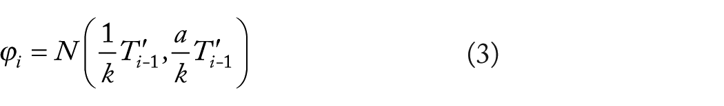
The formula says that the phase delay is sampled from a normal distribution whose mean is a fraction of the partner’s previous period, and whose standard deviation is proportional to that mean. In other words, the focal animal signals after its partner, with a time delay that is a fraction of the previous period of its partner. Parameter k can be interpreted as this fraction of a partner’s period equalling the focal’s delay. Biologically, k could be influenced by the speed of a species’ nervous system, from the moment a sound reaches an auditory organ to the moment a sound is produced. In behavioural and evolutionary terms, k could be influenced by the group density of a vocal display: for a species where choruses are always duets, one could expect k = 2, namely, alternation; with larger choruses (and shorter signals), one would expect a higher k. Parameter a quantifies the amount of jitter around the constant phase angle parameterised by k. So, for instance, in a duet with k = 2, as a tends to 0, the duet tends to perfect alternation. Conversely, a large a represents a loosely tuned mechanism; for a large enough, the focal animal times its signals almost independently from the conspecific.

In simulations of the antisynchrony model, the focal animal vocalises in the silences, possibly to enhance her conspicuousness and make itself heard. In contrast to the example of the frogs avoiding predation from a water snake provided above, the seal times its calls by moving away in time from the signals of its neighbour, and therefore increasing its conspicuousness. This results in antisynchrony and for seals it could be explained in evolutionary terms. Harbour seal pups produce mother attraction calls.^48–50 These calls are individually distinctive and calls of different pups can be easily discriminated by mothers a few days after birth. When mothers return from foraging and come back to their colony, they must identify the right pup. The seal pup, by vocalising in the silences, may make itself heard, facilitating individual recognition by the mother. This form of timing adjustment may thus play an important role in the dynamics of mother-pup recognition.^41,49,50

Figures 5 and 6 plot simulated data for the antisynchrony model as delay-period plots and rose plots. Both versions of the model, when visualised in delay-period plots (Figure 5), show a clear similarity to the arousal model (Figure 1) and difference from the phase-shift model (Figure 3). There is a main visual difference between antisynchrony and arousal: data points for antisynchrony are more clustered at lower values of the y-axis (shorter delays on average). This intuition becomes clear when comparing rose plots. Although the arousal rose plot (Figure 2) does not have a clear phase pattern, the antisynchrony rose plot (Figure 6) features a high number of observations at around 90°. This is consistent with the fixed phase angle described above.

Figure 5.

Antisynchrony model plotted using simulated data, showing lag-period plots for a simulated isochronous neighbour (left) and a constant-drift neighbour (right). In these graphs, the focal lag/delay (vertical) is plotted against the partner previous period (horizontal).

Figure 6.

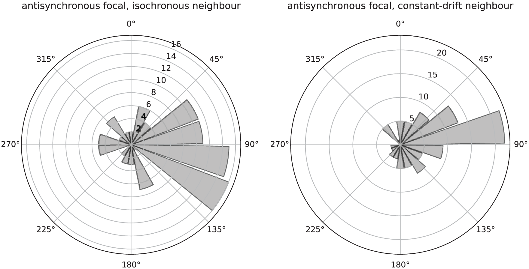
Rose plots of the antisynchrony model showing frequency distributions of relative phases, relative to a simulated isochronous neighbour (left) and a constant-drift neighbour (right).

Notice that the phase-delay model can yield either synchrony or antisynchrony depending on the parameters. In the phase-delay model, antisynchronous alternation arises if the animal ‘rebounds’ from inhibition rapidly (relative to its free-running period). So, why is an antisynchronous model needed? Among others, the main difference between the 2 models in explaining antisynchronous behaviour lies in their different tempo-dependent flexibilities. Although the phase-delay model will exhibit synchrony or antisynchrony only for a range of conspecific’s tempi, the antisynchrony will only exhibit antisynchronous behaviour, but for a much broader range of tempi.

Rhythmic Models in Humans: Period-Adjust/Linear Phase Correction in Music

Some rhythmicities such as breathing are generated at an endogenous neural level, but more complex rhythmic behaviours are dependent on externally supplied timing signals.¹⁰ The effector lag mentioned in the neural oscillator model is species-specific. However, this sensorimotor reaction time can be circumvented via proepisodic timing. For example, when humans gather in groups to sing and dance, they synchronise their voices and bodily movements to a shared, repeated timing interval, known as the (musical) beat.^51–54

Rhythmic behaviours in humans are frequently studied in the musical domain.⁵⁴ For instance, in ensemble musical performance, players do not always time their note onsets exactly as written on the score. This can be due to natural variation in timing abilities of each individual or because they introduce timing departures as a form of musical expressivity. Good auditory feedback information is thus needed to correct for the timing variations of other players. By adjusting their individual timings, the players restore relative phase with one another and maintain overall ensemble cohesion during performance. Wing et al³⁵ proposed a linear phase-correction model used for achieving synchrony in quartets. The asynchrony between a pair of note onsets produced by 2 performers is described as the phase error. Performers use this phase error to lengthen or shorten the time interval before the next tone onset. This ensures that the next pair of note onsets exhibits a smaller phase difference. The delay of the period-adjust model equals^35,55

φ_{i} = T_{i - 1} + c ({T^{'}}_{i - 1} - T_{i - 1})

(4)

In other words, the new signalling time of the focal individual equals its previous period length, adjusted to compensate the mismatch between the previous periods of focal and partner. Hence, if the focal’s previous period is shorter than the partner’s, the focal’s new period will be lengthened by a fraction of this difference. If, instead, the focal’s previous period is longer than the partner’s, the focal’s new period will be shortened by a fraction of this difference. Parameter c represents the ‘correction strength’³⁵: the magnitude of the effect that the mismatch in synchrony from the previous period has on the current period. For a low c, a previous asynchrony will only be minimally corrected in the current period. A high c will try to correct the previous asynchrony, with the risk of ‘overcorrecting’ it in the direction opposite to the previous asynchrony.

The linear phase-correction model produces asynchrony autocorrelation functions that match the output data and estimates the correction gain or strength for the pairs of players. Stable asynchrony time series can be described as those with gain changes between 0 and 2. Near-optimal improvement can be found across string quartets but contrasting patterns of adjustment between pairs of players exist. Two quartets were analysed in the string quartet study, which showed that 2 alternative mechanisms can be employed in music ensembles to maintain overall synchronisation.³⁵ In the first group, all players adjusted their timing to the leading player (see also Fuhrmann et al⁵⁶ for a non-human animal parallel). This copying mechanism suggests that copying the immediately preceding interval helps to maintain inter-individual synchrony. In the second group, the levels of gain correction of each player were similar. Synchronisation can therefore also be achieved by a central tendency or an average estimate of the prevailing unit duration over a number of previous beats in the sequence. This provides a more robust basis for period adjustment. Both mechanisms can coexist in generating a rhythmic behaviour. It is yet unknown how individuals switch between modes.

The simulated data for this model are plotted as delay-period scatterplots (Figure 7) and rose plots (Figure 8). Notice how, in both delay-period plots (Figure 7), the data points lie on, or close to, the 45° grey line. A point on this line represents an observation for which a focal individual responded with a delay identical to the previous period of the neighbour. Also, the rose plots (Figure 8) show a very clear picture. The relative phase is close to 0°, suggesting synchronisation. In addition, the slight negative asynchrony in Figure 8 curiously mirrors that found in human tapping studies.^57,58

Figure 7.

Period-adjust model plotted using simulated data, showing lag-period plots for a simulated isochronous neighbour (left) and a constant-drift neighbour (right). In these graphs, the focal lag/delay (vertical) is plotted against the partner previous period (horizontal).

Figure 8.

Rose plots of the period-adjust model showing frequency distributions of relative phases, relative to a simulated isochronous neighbour (left) and a constant-drift neighbour (right).

Rhythmic Models in Humans: Turn-Taking in Speech

Another example of rhythmic behaviour in humans is turn-taking during a conversation.⁵⁹ Although this mode of interaction has long been overlooked in language sciences,^59,60 mechanisms are in place to regulate when to speak. There are many different languages in the world and significant cultural differences can be found in the timing of turn-taking. Despite these differences, there exist clear universals in the pattern of response latency during conversation.⁶¹ The main opposing tendencies influencing response latency values are (1) avoidance of overlap and (2) minimisation of silences between turns.

Across languages, the time difference between an individual offset and another’s onset averages 229 ms.⁶¹ To achieve this close timing, speakers resort to prosody, pragmatics, and grammar to predict the timing of their turn.^59,60 Moreover, a speaker may pressure the listener to respond more quickly when directing his or her gaze towards the listener.

A crucial difference between turn-taking and the models discussed above is that speech is not, from a purely behavioural perspective, strictly periodic. The brain circuits underlying speech perception and production do engage in periodic oscillations.⁵⁴ The amplitude envelope of the speech signal shows some periodicities.^62,63 However, from a purely behavioural perspective, speech is much less periodic than, eg, (Western) music performance or insect choruses.⁵⁴ Some of the periodicity speakers perceive in the speech signal may in fact be subjectively induced via top-down cognitive processes.^54,64 The most objectively rhythmic feature of speech and language may actually lie in interactive turn-taking, rather than individual speech acts.^31,59,60,65 Although with extreme caution, we believe it is important to start developing computer simulations for turn-taking behaviour and compare them with a century of results from animal chorusing.^66,67 Below, we present the simplest possible model to simulate the rhythm of turn-taking, namely, a delay between speakers, calibrated using empirical findings from world languages. In our simple formulation, the delay of the turn-taking model equals⁶¹

φ_{i} = N (M_{S t i v}, S D_{S t i v})

(5)

where $M_{S t i v} = 229.485 a n d S D_{S t i v} = 512.99$ are estimates in milliseconds from cross-cultural human data by Stivers et al.⁶¹ In other words, the focal individual signals right after its partner, with a time delay that is randomly and normally distributed around the population’s delay. Analytically and prior to any simulation, when $M_{S t i v} = T$ and $b = S D_{S t i v} / M_{S t i v}$ , the turn-taking model is equivalent to the phase-delay model. Typically, however, human turn-taking will exhibit $b > 1$ , whereas insect phase-delay behaviour will exhibit $b < 1$ .

Notice that this very simple model makes many simplifications when abstracting away from the reality of turn-taking. In particular, it does not incorporate all the non-verbal signalling channels that enable an individual to predict when the neighbour’s signal will stop. Nonetheless, we stress the importance of incorporating turn-taking as a variation of animal chorusing, especially in discussions on the evolution of human behaviours.^66,67

Figures 9 and 10 plot simulated data for the turn-taking model as delay-period plots and rose plots. Both versions of the model, when visualised in delay-period plots (Figure 9) show some similarities to the arousal and antisynchrony models (Figures 1 and 5) and differences from the phase-shift and period-adjust models (Figure 3 and 7). This makes sense, because the latter 2 models are mechanisms used to achieve synchrony, whereas the 2 former models, together with turn-taking, either try to avoid synchrony or are neutral towards it. The rose plots (Figure 10) confirm and extend this intuition: there seem to be a tendency for the focal individual to signal 180° after the neighbour. It is unclear why this alternation pattern emerges and whether it is a simple by-product of the specific numerical parameters chosen in the simulation.

Figure 9.

Turn-taking model plotted using simulated data, showing lag-period plots for a simulated isochronous neighbour (left) and a constant-drift neighbour (right). In these graphs, the focal lag/delay (vertical) is plotted against the partner previous period (horizontal).

Figure 10.

Rose plots of the turn-taking model showing frequency distributions of relative phases, relative to a simulated isochronous neighbour (left) and a constant-drift neighbour (right).

Discussion and Conclusions

In this article, we (1) reviewed several models of interactive rhythm in animal communication, (2) formulated closed-form equations to describe them (3) simulated the dynamic behaviour of a hypothetical focal organism responding to a conspecific according to one of these signalling strategies, and (4) plotted the simulated data points using 2 visualisation techniques. A brief comparison of plots across models may be useful.

When compared using delay-period plots, each model has its own unique feature, but cross-model similarities also emerge. The arousal model (Figure 1) has a random relationship between x and y coordinates of each point: no particular trend is noticeable. The antisynchronous model (Figure 6), if observed alone and at first sight, would also appear quite random. However, when compared with the arousal plot, the antisynchronous plot shows a higher concentration of values with shorter delays (lower values for the y-coordinate). In fact, a hypothetical fit line would capture the variance of the linear relation (y = 0.25 × x) present in the lower point clusters of both plots in Figure 5. Notice that the fit would not be perfect because this simulation contains half of the data points generated with the antisynchronous mechanism and the other half generated via the arousal mechanism. Visually, the closest plot to Figures 1 and 5 is Figure 9, the turn-taking simulation. Figure 9 has, however, also a peculiar feature, namely, that delay values can be negative, meaning that the focal individual would signal before the neighbour, possibly overlapping with it. The 2 remaining models, the phase-delay (Figure 3) and period-adjusted (Figure 7), have a commonality that no other plots share: their data points lie close to or on the grey diagonal line. This similarity reflects their common underlying patterns when occurring in nature. Both models can explain quite well synchronous phenomena. A final feature is the potential similarity between Figures 3 and 9. The closed-form equations for the phase-delay and turn-taking models are actually equivalent up to scaling parameters. This equivalence is weak because it is based on the many simplifying assumptions of the models. However, it may be potentially informative of the fact that cooperative behaviour, which is not required in the phase-delay model but often assumed in turn-taking, may also be a minor factor when modelling turn-taking.⁶⁷

Comparing rose plots also shows some unique features of each model and similarities across them. The arousal model (Figure 2) has a random, almost evenly spread distribution around the circle. This spread is present, but reduced for turn-taking (Figure 10), and centred around approximately 180°. Similar, or less, spread appears in the phase-delay model (Figure 4), with the phase distribution centred at, or close to, 0°. Even less spread appears in the distributions of the remaining 2 models, the period-adjusted (Figure 8), centred close to 0°, and the antisynchronous model (Figure 6), centred close to 90°.

One key difference among models, which emerged through visualisation, is their propensity to produce or avoid synchronised behaviours. This is particularly evident when comparing rose plots (Figures 2, 4, 6, 8, and 10). Synchronisation, as seen in the phase-delay and period-adjust models, is achievable across species via both homoepisodic and proepisodic mechanisms. In music, prediction of the exact timing of the next signal via proepisodic mechanisms can enable synchronising to a specific tactus or beat. In the particular case of human musical rhythm, the structural grid of this isochronous pulse enables individuals to precisely time their rhythmic behaviour. A few animal species, with different evolutionary distances from humans, have a capacity to entrain to an isochronous pulse.^54,68–70 The best-known example can be found in a California sea lion (Zalophus californianus), named Ronan, that matched bobbing head movements to both simple and complex beats, and was capable of adjusting its timing in response to changes or perturbations.⁷¹ Its performance was well-captured by mathematical models of coupled oscillators.⁷¹ Comparative cross-species study of beat synchronisation can shed further light on the origin and evolution of flexible interactive timing.^70,72

This article is limited in its scope along a number of dimensions, namely: (1) it only reviews a small percentage of the literature on animal and human chorusing and turn-taking, while much more is available; (2) it limits interactive models to 2 individuals, while a critical aspect of rhythm interaction is the number of interacting agents; (3) it only adopts 1 type of computational approach to simulate agents, and 2 ways of visualising the outcomes of the simulations.

We have sketched the potential of adopting a computational approach in the behavioural study of animal rhythm and timing. We hope that the kind of modelling work we sketch here will serve as a baseline for future research, where computer simulations can help make predictions for, and compare results from, behavioural experiments.^13,41

Supplemental Material

Supplemental_Material – Supplemental material for Modelling Animal Interactive Rhythms in Communication

Supplemental material, Supplemental_Material for Modelling Animal Interactive Rhythms in Communication by Andrea Ravignani and Koen de Reus in Evolutionary Bioinformatics

Footnotes

Acknowledgements

The authors thank all members of the Sealcentre Pieterburen for the hospitality and continued support in research. The authors are also grateful to 4 anonymous reviewers for their insightful comments on a previous version of this article.

Funding:

The author(s) disclosed receipt of the following financial support for the research, authorship, and/or publication of this article: A.R. was supported by funding from the European Union’s Horizon 2020 research and innovation programme under the Marie Skłodowska-Curie grant agreement no. 665501 with the Research Foundation Flanders (FWO) (Pegasus² Marie Curie fellowship 12N5517N awarded to A.R.).

Declaration of conflicting interests:

The author(s) declared no potential conflicts of interest with respect to the research, authorship, and/or publication of this article.

Author Contributions

AR and KdR wrote the manuscript. All the authors jointly developed the structure and arguments for the paper, made critical revisions, and approved the final version.

Supplemental Material

Supplemental material for this article is available online.

References

Endler

Basolo

AL.

Sensory ecology, receiver biases and sexual selection. Trends Ecol Evol. 1998;13:415–420.

McGregor

PK.

Signalling in territorial systems: a context for individual identification, ranging and eavesdropping. Phil Trans R Soc Lond B. 1993;340:237–244.

Wiley

Richards

DG.

Physical constraints on acoustic communication in the atmosphere: implications for the evolution of animal vocalizations. Behav Ecol Sociobiol. 1978;3:69–94.

Dusenbery

. Sensory Ecology: How Organisms Acquire and Respond to Information. New York, NY: W. H. Freeman; 1992.

Yoshida

Okanoya

Evolution of turn-taking: a bio-cognitive perspective. Cogn Stud. 2005;12:153–165.

Andre

Kamminga

Rhythmic dimension in the echolocation click trains of sperm whales: a possible function of identification and communication. J Mar Biol Assoc. 2000;80:163–169.

Brumm

Signalling through acoustic windows: nightingales avoid interspecific competition by short-term adjustment of song timing. J Comp Physiol A. 2006;192:1279–1285.

Rosen

Temporal information in speech: acoustic, auditory and linguistic aspects. Phil Trans R Soc Lond B. 1992;336:367–373.

Collins

Stewart

IN.

Coupled nonlinear oscillators and the symmetries of animal gaits. J Nonlin Sci. 1993;3:349–392.

10.

Granada

Hennig

Ronacher

Kramer

Herzel

Phase response curves elucidating the dynamics of coupled oscillators. Methods Enzymol. 2009;454:1–27.

11.

Buck

Synchronous rhythmic flashing of fireflies. Quart Rev Biol. 1938;13:301–314.

12.

Buck

. Synchronous rhythmic flashing of fireflies. II. Quart Rev Biol. 1988;63:265–287.

13.

Greenfield

Roizen

Katydid synchronous chorusing is an evolutionarily stable outcome of female choice. Nature. 1993;364:618–620.

14.

Greenfield

Marin-Cudraz

Party

Evolution of synchronies in insect choruses. Biol J Linn Soc. 2017;122:487–504.

15.

Greenfield

Tourtellot

Snedden

WA.

Precedence effects and the evolution of chorusing. Proc Biol Sci. 1997;264:1355–1361.

16.

Backwell

Jennions

Passmore

Christy

Synchronized courtship in fiddler crabs. Nature. 1998;391:31–32.

17.

Grafe

TU.

A function of synchronous chorusing and a novel female preference shift in an anuran. Proc Biol Sci. 1999;266:2331–2336.

18.

Greenfield

Schul

Mechanisms and evolution of synchronous chorusing: emergent properties and adaptive functions in Neoconocephalus katydids (Orthoptera: Tettigoniidae). J Comp Psychol. 2008;122:289–297.

19.

Hall

ML.

A review of hypotheses for the functions of avian duetting. Behav Ecol Sociobiol. 2004;55:415–430.

20.

Greenfield

MD.

Cooperation and conflict in the evolution of signal interactions. Ann Rev Ecol Syst. 1994;25:97–126.

21.

Ravignani

Bowling

Kirby

The psychology of biological clocks: a new framework for the evolution of rhythm. Paper presented at: The Evolution of Language: Proceedings of the 10th International Conference; April 14-17, 2014; Vienna, Austria.

22.

Ravignani

Kotz

Evolution of temporal interaction: a comparative approach to social timing. PeerJ Preprint. 2017;5:e3275v1.

23.

Strogatz

Stewart

Coupled oscillators and biological synchronization. Sci Am. 1993;269:102–109.

24.

Pikovsky

Rosenblum

Kurths

Synchronization: A Universal Concept in Nonlinear Sciences. Vol 12. Cambridge, UK: Cambridge University Press; 2003.

25.

Ravignani

Visualizing and interpreting rhythmic patterns using phase space plots. Music Percept. 2017;34:557–568.

26.

Ravignani

Bowling

Fitch

WT.

Chorusing, synchrony and the evolutionary functions of rhythm. Front Psychol. 2014;5:1118.

27.

Oliveira

Melo

LV.

Huygens synchronization of two clocks. Sci Rep. 2015;5:11548.

28.

Winfree

AT.

The Geometry of Biological Time. Vol 12: Berlin, Germany: Springer; 2001.

29.

Ravignani

Interdisciplinary debate: agree on definitions of synchrony. Nature. 2017;545:158–158.

30.

Ravignani

. Comment on ‘Temporal and spatial variation in harbor seal (Phoca vitulina L.) roar calls from southern Scandinavia’ [J. Acoust. Soc. Am. 141, 1824-1834 (2017)]. J Acoust Soc Am. 2018;143:504.

31.

Ravignani

Madison

The paradox of isochrony in the evolution of human rhythm. Front Psychol. 2017;8:1820.

32.

Bailey

WJ.

Insect duets: underlying mechanisms and their evolution. Physiol Entomol. 2003;28:157–174.

33.

Snow

. Duetting and other synchronised displays of the blue-backed manakins, Chiroxiphia spp. In: Stonehouse

Perrins

(eds) Evolutionary Ecology. London, England: Palgrave; 1977:239–251.

34.

Walker

TJ.

Acoustic synchrony: two mechanisms in the snowy tree cricket. Science. 1969;166:891–894.

35.

Wing

Endo

Bradbury

Vorberg

Optimal feedback correction in string quartet synchronization. J R Soc Interface. 2014;11:20131125.

36.

Mann

Dingess

Slater

Antiphonal four-part synchronized chorusing in a Neotropical wren. Biol Lett. 2006;2:1–4.

37.

Patel

Iversen

Bregman

Schulz

Studying synchronization to a musical beat in nonhuman animals. Ann N Y Acad Sci. 2009;1169:459–469.

38.

Allman

Teki

Griffiths

Meck

WH.

Properties of the internal clock: first-and second-order principles of subjective time. Ann Rev Psychol. 2014;65:743–771.

39.

Matell

Meck

WH.

Neuropsychological mechanisms of interval timing behavior. Bioessays. 2000;22:94–103.

40.

Large

. Resonating to musical rhythm: theory and experiment. Psychol Time. 2008:189–232.

41.

Ravignani

. Timing of antisynchronous calling: a case study in a harbor seal pup (Phoca vitulina) [published online ahead of print December 13, 2018]. J Comp Psychol. doi:10.1037/com0000160.

42.

Peskin

CS.

Mathematical Aspects of Heart Physiology. New York, NY: Courant Institute of Mathematical Sciences; 1975.

43.

Mirollo

Strogatz

SH.

Synchronization of pulse-coupled biological oscillators. SIAM J Appl Math. 1990;50:1645–1662.

44.

Strogatz

SH.

Sync: The Emerging Science of Spontaneous Order. New York, NY: Hyperion; 2003.

45.

Buzsaki

Rhythms of the Brain. Oxford, UK: Oxford University Press; 2006.

46.

Hamilton

WD.

Geometry for the selfish herd. J Theor Biol. 1971;31:295–311.

47.

Ravignani

Chronometry for the chorusing herd: Hamilton’s legacy on context-dependent acoustic signalling – a comment on Herbers (2013). Biol Lett. 2014;10:20131018.

48.

Ravignani

Kello

de Reus

et al . Ontogeny of vocal rhythms in harbour seal pups: an exploratory study. Curr Zool. 2018; 1–14.

49.

Sauvé

Beauplet

Hammill

Charrier

Mother–pup vocal recognition in harbour seals: influence of maternal behaviour, pup voice and habitat sound properties. Anim Behav. 2015;105:109–120.

50.

Sauvé

Beauplet

Hammill

Charrier

Acoustic analysis of airborne, underwater, and amphibious mother attraction calls by wild harbor seal pups (Phoca vitulina). J Mammal. 2015;96:591–602.

51.

Fitch

WT.

Rhythmic cognition in humans and animals: distinguishing meter and pulse perception. Front Syst Neurosci. 2013;7:68.

52.

Fitch

. The biology and evolution of musical rhythm: an update. In: Toivonen

Csúri

van der Zee

(eds) Structures in the Mind: Essays on Language, Music, and Cognition in Honor of Ray Jackendoff. Cambridge, MA: The MIT Press; 2015:293–324.

53.

Fitch

WT.

Dance, music, meter and groove: a forgotten partnership. Front Hum Neurosci. 2016;10:64.

54.

Kotz

Ravignani

Fitch

WT.

The evolution of rhythm processing. Trends Cogn Sci. 2018;22:896–910.

55.

Merker

Madison

Eckerdal

On the role and origin of isochrony in human rhythmic entrainment. Cortex. 2009;45:4–17.

56.

Fuhrmann

Ravignani

Marshall-Pescini

Whiten

Synchrony and motor mimicking in chimpanzee observational learning. Sci Rep. 2014;4:5283.

57.

Repp

BH.

Sensorimotor synchronization: a review of the tapping literature. Psychon Bull Rev. 2005;12:969–992.

58.

Repp

Y-H.

Sensorimotor synchronization: a review of recent research (2006-2012). Psychon Bull Rev. 2013;20:403–452.

59.

Holler

Kendrick

Casillas

Levinson

SC.

Turn-taking in human communicative interaction. Front Psychol. 2015;6:1919.

60.

de Vos

Torreira

Levinson

. Turn-timing in signed conversations: coordinating stroke-to-stroke turn boundaries. Front Psychol. 2015;6:268.

61.

Stivers

Enfield

Brown

et al . Universals and cultural variation in turn-taking in conversation. Proc Natl Acad Sci U S A. 2009;106:10587–10592.

62.

Leong

Goswami

Impaired extraction of speech rhythm from temporal modulation patterns in speech in developmental dyslexia. Front Hum Neurosci. 2014;8:96.

63.

Leong

Goswami

Acoustic-emergent phonology in the amplitude envelope of child-directed speech. PLoS ONE. 2015;10:e0144411.

64.

Jadoul

Ravignani

Thompson

Filippi

de Boer

Seeking temporal predictability in speech: comparing statistical approaches on 18 world languages. Front Hum Neurosci. 2016;10:586.

65.

Levinson

Torreira

Timing in turn-taking and its implications for processing models of language. Front Psychol. 2015;6:731.

66.

Pika

Wilkinson

Kendrick

Vernes

SC.

Taking turns: bridging the gap between human and animal communication. Proc R Soc B. 2018;285:20180598.

67.

Ravignani

Rhythm and synchrony in animal movement and communication. Curr Zool. 2018;1–5. https://doi.org/10.1093/cz/zoy087

68.

Cook

Rouse

Wilson

Reichmuth

CJ.

A California sea lion (Zalophus californianus) can keep the beat: motor entrainment to rhythmic auditory stimuli in a non vocal mimic. J Comp Psychol. 2013;127:412–427.

69.

Patel

Iversen

Bregman

Schulz

Experimental evidence for synchronization to a musical beat in a nonhuman animal. Curr Biol. 2009;19:827–830.

70.

Ravignani

Cook

The evolutionary biology of dance without frills. Curr Biol. 2016;26:R878–R879.

71.

Rouse

Cook

Large

Reichmuth

Beat keeping in a sea lion as coupled oscillation: implications for comparative understanding of human rhythm. Front Neurosci. 2016;10:257.

72.

Wilson

Cook

PF.

Rhythmic entrainment: why humans want to, fireflies can’t help it, pet birds try, and sea lions have to be bribed. Psychon Bull Rev. 2016;23:1647–1659.

Supplementary Material

Please find the following supplemental material available below.

For Open Access articles published under a Creative Commons License, all supplemental material carries the same license as the article it is associated with.

For non-Open Access articles published, all supplemental material carries a non-exclusive license, and permission requests for re-use of supplemental material or any part of supplemental material shall be sent directly to the copyright owner as specified in the copyright notice associated with the article.

0.00 MB

0.09 MB