Sage Journals: Discover world-class research

Abstract

The accurate estimation of nucleotide variability using next-generation sequencing data is challenged by the high number of sequencing errors produced by new sequencing technologies, especially for nonmodel species, where reference sequences may not be available and the read depth may be low due to limited budgets. The most popular single-nucleotide polymorphism (SNP) callers are designed to obtain a high SNP recovery and low false discovery rate but are not designed to account appropriately the frequency of the variants. Instead, algorithms designed to account for the frequency of SNPs give precise results for estimating the levels and the patterns of variability. These algorithms are focused on the unbiased estimation of the variability and not on the high recovery of SNPs. Here, we implemented a fast and optimized parallel algorithm that includes the method developed by Roesti et al and Lynch, which estimates the genotype of each individual at each site, considering the possibility to call both bases from the genotype, a single one or none. This algorithm does not consider the reference and therefore is independent of biases related to the reference nucleotide specified. The pipeline starts from a BAM file converted to pileup or mpileup format and the software outputs a FASTA file. The new program not only reduces the running times but also, given the improved use of resources, it allows its usage with smaller computers and large parallel computers, expanding its benefits to a wider range of researchers. The output file can be analyzed using software for population genetics analysis, such as the R library PopGenome, the software VariScan, and the program mstatspop for analysis considering positions with missing data.

Keywords

Population genomics SNP caller next-generation sequencing parallelization HPC MPI

Introduction

The analysis of genome variability using next-generation sequencing (NGS) data has been successfully performed in many species, mainly in model species where large read depth was usually achieved and the reference sequence for that species was available.^1–6

However, the study of nonmodel organisms becomes a challenge when the reference sequence is not available and exists the reference of a related species. Moreover, research projects trying to engage population genomics analysis of nonmodel species with limited budgets are forced to choose between few individuals at relative high read depth or, alternatively, to more individuals but moderate to low read depth.

Popular NGS pipelines for calling single-nucleotide polymorphisms (SNPs) are not always adequate for population genomics analyses and should be used with caution. Previous publications^7–11 show that important errors are introduced during the estimation of the levels and the patterns of variability under common experimental designs,¹² moderate or low read depth and/or nonreference species.

Bioinformatic tools for the analysis of variants from NGS data have been mainly designed for detecting SNPs but not for the analysis of variability. Accurate estimation of the levels of variability has fundamental importance for the detection of selective events and for understanding the history of the populations. Most popular SNP callers^6,13 are mainly focused on the high recovery detection of SNPs while keeping lower false discovery rates. Li⁶ developed a statistical framework for SNP calling, which accurately assigns the frequency spectrum of the alleles using a likelihood ratio test. Although this algorithm is effectively efficient for large sample data sets and even for low read depths, the frequency of the variants deviates from the expected value for small data sets, especially when divergent reference sequences are used.¹⁰ Furthermore, the number of missing positions (positions without information about the nucleotide are present there) in regions with no variants has not been specifically taken into account in most variability analyses. In summary, estimates of variability can be very far from the real one because the inaccurate frequency of the variants and the unclear information about the effective positions to be considered for the analysis.

In this work, we present a new version of the software GH caller. GH caller reads pileup and mpileup format files and outputs a FASTA format file ready to be analyzed by different software tools for the study of population genomics, such as PopGenome,¹⁴ VariScan,¹⁵ and mstatspo.¹⁰ It implements the Roesti et al¹⁶ and Lynch¹⁷ algorithm to accurately account the number of effective positions and the frequency of the variants, making this tool highly suitable for population genomics studies, especially at low read depths where it outperforms alternative SNP callers such as SAMtools or GATK (see the work by Nevado et al¹⁰). This new version of GH caller has been mainly developed to obtain results in a reasonable time, which in the field of NGS analysis is critical. In this sense, GH caller has been optimized for faster processing in 2 ways: (1) modifying the code algorithm and (2) using several high-performance computing (HPC) strategies.

Methods

Features of GH caller

GH caller is a tool for genome variability analysis that reads NGS mapped reads from diploid individual(s) in a pileup or mpileup file, performs SNP calling as developed by Roesti et al,¹⁶ and outputs the results in a multi-FASTA file. For each individual and site, 2 bases are represented, including missing values (N) if any, as they contain the diploid information available for each homologous position. GH caller counts the number of chromosomes that are effectively read per site making the frequency estimation unbiased in relation to the sample, which is useful for calculating neutrality tests and nucleotide variation.¹⁰

Input and output data

GH caller reads mpileup or pileup formats obtained from BAM standard NGS files using SAMtools.¹⁸ The first 3 columns represent the chromosome or scaffold name, the position number, and the reference sequence, respectively. The rest of columns are grouped in sets of 3 elements, representing the data of a diploid individual with the number of reads, the bases seen, and the base quality. The pileup format contains information for a single individual, whereas mpileup can contain data from multiple individuals. The name of each individual can be included using the flag –names to help the identification of the sequences. Also, the optional out-group sequence can be appended in the same FASTA file using the flags (–outgroup; see Supplementary Table 1 for more options). Note that each pileup file and each FASTA reference file must contain a single chromosome. Also, mpileup data should be filtered for mapping quality, to avoid reads with very low mapping quality introducing errors.

The output of GH caller is a multi-FASTA format file with 2 sequences per individual and a length equal to the same length as the input scaffold/chromosome. Each 2 consecutive sequences represent the unphased genotype of each individual.

Algorithm

Frequency caller algorithm for diploid samples

GH caller implements the Roesti algorithm,¹⁶ which is based on the algorithms proposed by Lynch¹⁷ and Hohenlohe et al.¹⁹ In this implementation, a preliminary filtering is convenient for erasing the possible noise produced by very-low-quality sequencing data but also for regions where the numbers of reads were disproportionally high or too low to be used for the variability estimation. In Supplementary Table 1, the filtering options available are described. The American Standard Code for Information Interchange (ASCII) code for each used sequencing platform (flag –platform) can also be included to calculate the quality of the sequences appropriately.

The Roesti algorithm implemented in GH caller calculates the genotype of each site and individual with a multinomial (see equations (1) to (3) below), assuming a fixed raw sequence error (flag –error). The 2 most likely genotypes are compared with a likelihood ratio test (LRT) against a χ² distribution (flag –chivalue) as indicated in the algorithm proposed by Hohenlohe et al. In the case LRT is not significant or the number of reads is below a threshold (eg, flag –minreads = 6), GH caller calculates the likelihood of a single nucleotide (so defines 1 of the 2 nucleotides to estimate as N). Likelihood ratio test is performed for the 2 most likely of the 4 remaining possibilities (A/N, C/N, T/N, and G/N). If significant, it keeps the one with the highest probability; otherwise, it assigns N/N. In a more formal notation, the detailed algorithm explained above is described as follows.

Define $n_{r}$ as the number of reads that pass the base quality threshold per site and per individual. Define minreads as the minimum number of reads to attempt a genotype call.

If $n_{r} \geq minreads$ do (A), otherwise do (B).

(A)—Define all 10 possible genotypes for 4 different nucleotides, ie, AA, AC, CC, AG, CG, GG, AT, CT, GT, and TT. As indicated in equations (1a) and (1b) by Hohenlohe et al,¹⁹ for a given nucleotide, namely, $1,2,3, or 4$ and a number of reads for each nucleotide $n_{r 1}$ , $n_{r 2}$ , $n_{r 3}$ , and $n_{r 4}$ , define $ε$ as a given raw sequence error rate, then the likelihood to have a heterozygous genotype (1, 2) is as follows:

\begin{array}{l} L (1, 2) = \\ \frac{n_{r}!}{n_{r 1}! n_{r 2}! n_{r 3}! n_{r 4}!} {(0.5 - \frac{ε}{4})}^{n_{r 1}} {(0.5 - \frac{ε}{4})}^{n_{r 2}} {(\frac{ε}{4})}^{n_{r 3}} {(\frac{ε}{4})}^{n_{r 4}} \end{array}

(1)

and the likelihood to be homozygous is as follows:

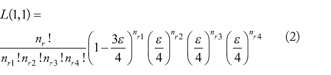
\begin{array}{l} L (1, 1) = \\ \frac{n_{r}!}{n_{r 1}! n_{r 2}! n_{r 3}! n_{r 4}!} {(1 - \frac{3 ε}{4})}^{n_{r 1}} {(\frac{ε}{4})}^{n_{r 2}} {(\frac{ε}{4})}^{n_{r 3}} {(\frac{ε}{4})}^{n_{r 4}} \end{array}

(2)

Calculate all 10 combinations and choose the 2 genotypes with the highest likelihood, namely, $L_{g 1}$ and $L_{g 2}$ .

If $L R T = - 2 \log (L_{g 2} / L_{g 1}) > χ_{p}^{2}$ , keep the highest likelihood genotype $(L_{g 1})$ , where $χ_{p}^{2}$ is the threshold $χ^{2}$ value, given by the user for a 1-degree-of-freedom test. Otherwise, do step B.

(B)—Call only one of the nucleotides of the genotype, leaving the remaining a missing site (N). The likelihood is as follows:

\begin{array}{l} L (1, N) \\ = \frac{n_{r}!}{n_{r 1}! n_{r 2}! n_{r 3}! n_{r 4}!} {(1 - \frac{3 ε}{4})}^{n_{r 1}} {(\frac{ε}{4})}^{n_{r 2}} {(\frac{ε}{4})}^{n_{r 3}} {(\frac{ε}{4})}^{n_{r 4}} \end{array}

(3)

Calculate all 4 combinations (ie, N and each of the 4 nucleotides) and choose the 2 haplotypes with the highest likelihood, namely, $L_{h 1}$ and $L_{h 2}$ .

If $L R T = - 2 \log (L_{h 2} / L_{h 1}) > χ_{p}^{2}$ , keep the highest likelihood haplotype ( $L_{h 1}$ , ie, (1, N)), where $χ_{p}^{2}$ is the threshold $χ^{2}$ value given by the user for a 1-degree-of-freedom test. Otherwise, keep the missing genotype (N, N).

Parallel algorithm

The parallel implementation is based on a previous serial version of GH caller.¹⁰ The new approach takes advantage of the inherent data parallelism existing in the algorithm, where all the steps can be applied for each position. Thanks to this property, we can split input data in groups of $n$ positions and distribute them among the available processing units, where all computations will be performed concurrently. The main phases of the parallel program are as follows:

All the involved processes initialize the parallel environment.

The main process (master) indexes the input file, generates a list of chunks of data to be assigned, and maps the corresponding piece of input data to the other processes (workers).

The parallel computations start asynchronously on each worker. Locally, each process reads and parses a subset of data, applies the base calling algorithm to these data, and finally writes its partial results to the final FASTA output file.

If it was selected as a command line option, a synchronization point (barrier) is used to allow the master process to append a reference/out-group sequence to the FASTA output file.

Phases 1 and 3 are independent and only need a synchronization signal to begin, hence are performed in parallel, whereas phases 2 and 4 are serial and must be performed in order in a single master process. This sequence of steps is shown in Figure 1 as a flowchart of the parallel algorithm.

Figure 1.

Flowchart of the master/worker algorithm, a parallel implementation of the Roesti algorithm.

Our application uses the standard Message Passing Interface (MPI)²⁰ and distributes the data among the available processes by mapping subsets of data with a default size of 100 MB (hereinafter “chunks”), giving 1 chunk to each worker process at a time. All computational tasks involving these data subsets can be performed simultaneously and individually on each worker process. Each chunk does not need to be replicated in the local memory of other processes, and memory used is released when data are written to disk: this allows GH caller to process data sets without any size limits and use all the aggregated memory available of all the allocated processors, at the same time.

Accuracy of results and usage of computational resources

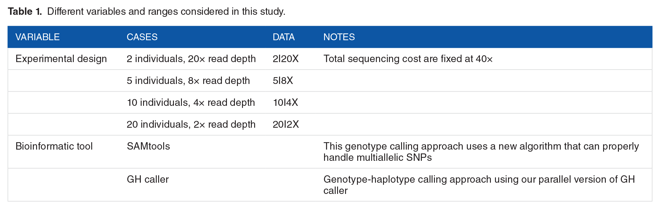
We had the following goals in our experiments: (1) accuracy of results and (2) usage of computational resources. First, we contrasted the serial and the parallel versions to validate all the changes introduced to the initial algorithm and thus to be sure both applications produce exactly the same results. Second, to analyze the computer performance of this new improved algorithm, we considered NGS data in several scenarios with a single population. The NGS sequences from the western lowland gorilla Gorilla gorilla²¹ were used for this purpose. As in the study by Nevado et al,¹⁰ already mapped files to gorilla genomes constructed in this previous work were subsampled using picard-tools DownsampleSam.²² To obtain all BAM files used in this work as input data, we kept the total sequencing costs fixed but sampling a varying number of individuals (diploid) with different read depth levels. As a result, each individual has a BAM file with a read depth level in a range of 2 to 20 while keeping total sequencing costs fixed at 40× (see Table 1 for more details of the different variables and the ranges considered). We estimated population genome-wide statistics from this data set to compare the overall accuracy of our application versus the new comparable algorithm provided by SAMtools.^6,23 In addition, we have compared the results of GH caller and SAMtools in a set of real data sequences²⁴. Here, we have analyzed 6 different lines (VED, IRK, SC, CAL, TRI, and CV) of Cucumis melo and 1 out-group (cucumber, ie, Cucumis sativus). From these lines, we have decided to use the chromosome 1 data set, as is large enough to perform a comparative analysis. We have used 2 different pipelines, both starting from individual pileup files for each variety. First, we used the SAMtools pipeline (as is detailed in the original manuscript of Sanseverino et al²⁴) to obtain all estimated SNPs. Following the original manuscript, the SNP file containing all the information was converted into a single multi-FASTA file. Second, we used GH caller to estimate the number and the frequency of the SNPs from pileup files. GH caller outputs FASTA files that were were concatenated into a single one. After that, the 2 multi-FASTA files (1 from SNP calling with SAMtools and 1 from SNP calling of GH caller) were analyzed using mstatspop (available from NumGenomics Web site, http://bioinformatics.cragenomica.es/numgenomics/people/sebas/software/software.html) to obtain the levels and patterns of variability. Finally, we have quantified the benefits from parallelization and optimization done in this application, and we have evaluated the overall effectiveness of the application, particularly, assessing how it can scale across different computing platforms.

Table 1.

Different variables and ranges considered in this study.

Variable	Cases	Data	Notes
Experimental design	2 individuals, 20× read depth	2I20X	Total sequencing cost are fixed at 40×
	5 individuals, 8× read depth	5I8X
	10 individuals, 4× read depth	10I4X
	20 individuals, 2× read depth	20I2X
Bioinformatic tool	SAMtools		This genotype calling approach uses a new algorithm that can properly handle multiallelic SNPs
	GH caller		Genotype-haplotype calling approach using our parallel version of GH caller

SAMtools pipeline

We used the well-known package SAMtools to compare results against our GH caller pipeline. In our pipeline, each individual’s data are analyzed separately. We used version 1.2.0 that includes an algorithm to properly handle multiallelic SNPs.^6,23 Figure 2A shows the main steps of the pipeline.

Figure 2.

SNP calling and filtering pipelines used in our experiments. (A) In case of SAMtools’ pipeline, all steps are repeated for each individual. One extra step is needed to convert VCF output obtained in step 3 to a FASTA format input file required by mstatspop. (B) In case of GH caller, the output file obtained in step 2 is already produced in the required format.

We started with the SAMtools’ command, SAMtools mpileup (step 1), computing genotype likelihoods (-g), reading a maximum of 1000 reads per-position (-d 1000), and using both minimum base quality threshold and minimum mapping quality of 20, and disabling the probabilistic realignment for the computation of base alignment quality (BAQ), which helps to reduce false SNPs’ discoveries caused by misalignments. We instruct the program to generate an uncompressed output (-u), choosing a list of tags as output format (-t): number of high-quality bases (DP), per-sample Phred-scaled strand bias P value (SP), number of high-quality nonreference bases (SP), and number of high-quality ref-forward, ref-reverse, alt-forward, and alt-reverse bases (DP4). All other options were kept with their default values.

For analysis with SAMtools, we used the BCFtools call command (step 2a) with the new multiallelic and rare-variant calling algorithm (-m) (http://samtools.github.io/bcftools/call-m.pdf) and aggregating to the output also gVCF blocks of homozygous reference calls, where the minimum depth (-g) should be set to half the depth in each scenario. Variant calls were filtered with bcftools filter command of SAMtools package (step 2b), with the following options (-saFilter -g3 -G10) and a exclude expression (-e) which marks as low-quality SNPs those with quality below 10 (%QUAL < 10) or 15 if less than 2 reads support alternative base (AC < 2 && %QUAL < 15), and those with a minimum depth below threshold, which should be half the average depth for each scenario (FMT/DP < “$MINDEP”).

The new filtered VCF format file was transformed to FASTA format using vcf2fasta (available from GitHub, https://github.com/brunonevado/vcf2fas). Finally, FASTA output files were analyzed with mstatspop.

GH caller pipeline

Figure 2B shows the main steps of this pipeline. We started the pipeline with a SAMtools’ mpileup command (step 1), using a minimum base quality threshold and a minimum mapping quality, both with a value of 20 and disabling the probabilistic realignment for the computation of BAQ. Other tool settings are kept with their default values. To start applying a genotype-haplotype per base calling, we run GH caller (step 2) with a set of options similar to the previous work: we used a threshold of 6 reads for genotype calls (–minreads = 6) and we only considered bases with a base quality above 20 (–baseq = 20). Moreover, for each position and individual, we discarded sites having above double and below half the average read depth. That is, for data with an average read depth of 20× we would discard positions above 40 and below 10 reads (–maxdep = 40, –mindep = 10). We set the raw sequencing error used to calculate the genotype/haplotype likelihoods to 0.01 (–error = 0.01) (see the algorithm above and the definition of the error parameter in the equations). Finally, as parameter to apply the LRT, we set the χ² distribution to its default value (see options in Supplementary Table 1).

Estimating population genetics statistics

The different statistics of variability allow us to detect differences in the patterns of expected variability considering different aspects of the site frequency spectrum, ie, low, intermediate, or high SNP frequencies, and detect possible biases. The variability estimators of Watterson (θ_w),²⁵ Tajima²⁶ (π), Achaz²⁷ (θ_A), Fay and Wu²⁸ (θ_H), and Fu and Li²⁹ (θ_FL), were calculated over windows of 100 kB for the entire chromosome. Also, the neutrality tests of Tajima³⁰ (TD), Fu and Li²⁹ (D FLD), and Fay and Wu²⁸ (H) were considered. Population statistics were calculated using the mstatspop tool from NumGenomics Web site in both pipelines (Figure 2, step 3).

Computing performance

We used a hetereogeneous cluster, which consists of 2 groups of nodes with different hardware configurations. As first hardware configuration (scenario A), we chose 1 server with 1 processor Intel Xeon E31240 with frequency 3.30 GHz providing 4 cores with 2 threads per core, 32 GB of RAM and running the operating system Scientific Linux 6.3. In this scenario, our application was evaluated using a local file system (XFS) using 1 internal SATA hard drive of 3 TB. This scenario is equivalent in terms of computational power to current workstation computers. The second configuration (scenario B) is composed by 6 servers or nodes. Each node has 2 processors Intel Xeon X5660 processors with frequency 2.8 GHz providing 6 cores per processor with 2 threads per core, 96 GB of RAM, and running the same Linux distribution than scenario A. All these 6 nodes were connected via network links of 10 GB Ethernet. In this scenario, our application was evaluated using the distributed file system Lustre version 2.5.3, configured with 1 Metadata Server and 2 object storage servers, which were connected to the same network switch. This scenario represents typical shared clusters found in many research centers. In both scenarios, we used mpicxx for Open MPI version 1.8.8, and gcc 4.9.1 to compile all the source codes, with -03 optimization enabled.

The performance of GH caller is evaluated using the execution time $(T)$ as a metric measured in seconds. In our case, execution time $(T)$ is the maximum amount of time the application could take to execute on a specific hardware platform. $T_{1}$ is essentially the execution time of the original GH caller application (serial) using only 1 core as computational resources, $N$ is the number of cores, and $T_{N}$ is the running time of the parallel algorithm using $N$ cores.

First, we compared the execution time elapsed with our new parallel version $(T_{N})$ using both scenarios (A and B) while keeping the same workload and increasing the number of resources (N). Next, we ran the serial version of GH caller with all data sets, so we obtained $T_{1}$ as a baseline time $T$ to compare gains obtained at different times $T_{N}$ . We performed each experiment 10 times for each pileup input file and measured the time of program execution. Average execution time is calculated taking these 10 replicates.

Memory usage

The memory usage of GH caller is evaluated using the maximum resident set size (RSS memory) for each process during program execution. Resident set size is used to show how much of the memory allocated for a process is currently in main memory, including both stack and heap memory. It does not include neither swap nor memory used by shared libraries as long as the pages from those libraries were currently in memory. We obtained all these values using the accounting tool sacct provided by SLURM (Simple Linux Utility for Resource Management),³¹ the software used in the cluster to manage all the jobs submitted by the users. The sacct command displays accounting data for all jobs and job steps in the SLURM job accounting database in a variety of forms for analysis.

To identify the impact in memory usage caused using subsets of data with a restricted size, we evaluated our application choosing the default chunk size of 100 MB and compared our results with the serial version of GH caller to find whether there are any gains obtained with respect to the original. In this case, we used only scenario A to run our experiment due to the fact that the differences between hardware in both scenarios should have no impact in memory usage. We launched the same experiments 5 times for each pileup input file and obtained the maximum RSS memory for each process measured by the SLURM accounting system during program execution. An average RSS memory size is calculated by taking all execution replicates.

Results

Accuracy of optimized GH caller versus updated SAMtools SNP caller

In the same direction to what was described by Nevado et al¹⁰ for a previous SAMtools version, there is a strong dependency of SAMtools SNP caller to the average read depth when the level of variability and frequency-dependent neutrality tests are estimated, and it is much less dependant in the case of GH caller (Figures 3 and 4 and Supplementary Figures 4 and 5). As it can be observed, there are no changes in the results of the parallel version with respect to the accuracy of the original GH caller. In case of the second real data analysis (Figures 3 and 4), it is observed that the SAMtools SNP caller has much stronger correlation between levels of variability, and the variance in the read depth per window is compared, suggesting that the differences in the levels of variability and the patterns of variability between GH caller and SAMtools are consequence of artefactual patterns not well considered using the SAMtools SNP caller.

Figure 3.

The levels of variability for different statistics of variability (Theta Watterson, Theta Fu&Li, and Theta Fay&Wu) are estimated per windows of 100 MB across the chromosome 1 using SAMtools (blue) and GH caller (red).

Figure 4.

Correlation of the levels of variability and the variance in the number of read depths per individual. The levels of variability for different statistics of variability (Theta Watterson, Theta Fu&Li, and Theta Fay&Wu from left to right) are estimated per windows of 100 MB across the chromosome 1 using SAMtools (upper plots in blue) and GH caller (bottom plots in red). A significant value indicates that the estimated variability is dependent on the read depth.

Usage of computational resources

The main objective of the experiments described here is to demonstrate the utility of the new application for the analysis of variability by improving the usage of computational resources. To obtain all input files used to benchmark our application, we converted all alignment BAM files to mpileup format with different read depth levels and number of individuals required.

Computing performance

Table 2 shows the real time elapsed running GH caller in scenarios A and B. It can be clearly observed that the total execution time decreases by including more computational resources in both scenarios.

Table 2.

Execution time running GH caller in scenarios A (workstation) and B (cluster).

Data	Size, GB	Scenario A, No. of cores		Scenario B, No. of cores
Data	Size, GB	2	4	2	4	8	16	32	64
2I20X	14	7 m 44 s	3 m 00 s	7 m 16 s	2 m 34 s	1 m 15 s	54 s	49 s	46 s
5I8X	16	12 m 40 s	4 m 38 s	12 m 24 s	4 m 20 s	2 m 04 s	1 m 32 s	1 m 03 s	58 s
10I4X	18	21 m 32 s	7 m 43 s	21 m 44 s	7 m 27 s	3 m 46 s	2 m 23 s	1 m 32 s	1 m 20 s
20I2X	20	35 m 26 s	12 m 53 s	38 m 29 s	13 m 08 s	6 m 29 s	3 m 50 s	2 m 21 s	1 m 52 s

Supplementary Figure 1 shows the results from the experiments performed in scenario A (workstation). In this experiment, we scaled up to the total number of cores available in this server (4 cores) performing an SNP calling process over all data sets (2I20X, 5I8X, 10I4X, and 20I2X). This results in an elapsed time reduced from 35 minutes 26 seconds (2 cores) to 12 minutes 53 seconds (4 cores), which is a 2.5× decrease using the same input data (20I2X). However, potential gains are being limited due the lack of processing units.

The second set of experiments has been performed in scenario B (cluster). In this case, we scaled up to a maximum of 64 cores (6 nodes). Supplementary Figure 2 shows how execution time can be reduced up to 20× (20I2X) by adding more computational resources. We can observe how efficiency decreases when scaling up computational resources, the reason of which will be discussed in the next section.

Finally, Figure 5 compares execution time of GH caller using the original version with 1 core versus the parallel version using up to 64 cores over all data sets. Looking at the figure, we can conclude that regardless of input data, execution time can be reduced using the parallel version of GH caller together with all the available resources.

Figure 5.

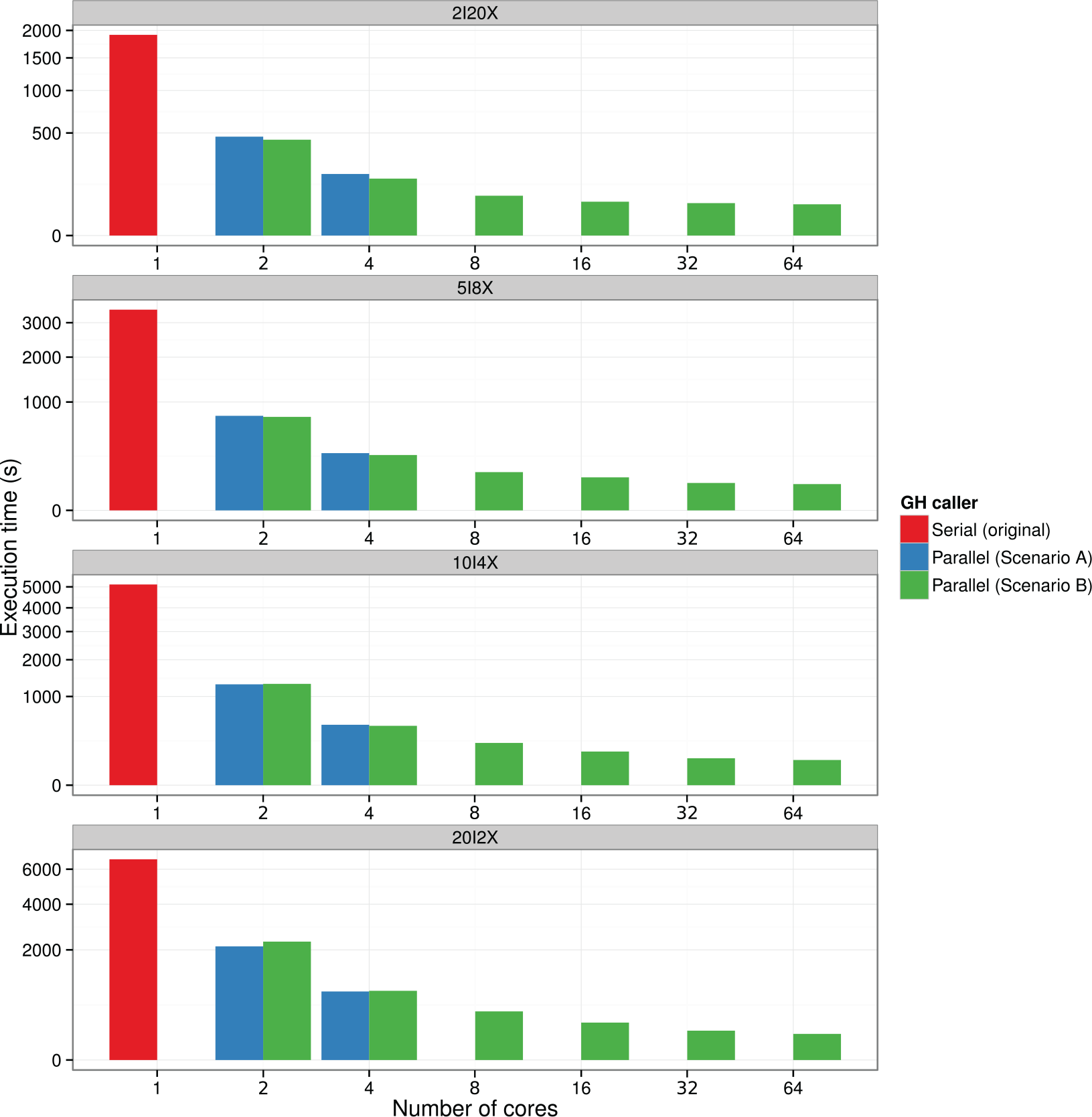
Comparison of execution times using the original version with 1 core versus the parallel version using all the available cores in both scenarios A and B. We run an SNP calling process over all data sets (2I20X, 5I8X, 10I4X, and 20I2X). In all cases, execution time can be reduced using this parallel version of GH caller, especially using all resources from scenario B (cluster).

In conclusion, we can see that there is a significant reduction at the total execution time used by this new version of GH caller in both scenarios, especially with data sets with highest number of individuals.

Memory usage

Table 3 shows the results of executing both GH caller serial (1 core) and parallel (64 cores) with input data of different sizes. As we can observe in the first column, previous serial version of GH caller increases memory consumption accordingly to the size of input data: this version uses a maximum RSS memory size of 0.64 GB with an input data of 14 GB (case 2I20X) but more than 5 GB with an input of 20 GB (20I2X). As it is expected, it increases memory usage in 10× because the number of sequences analyzed is 10 times more when using data set 2I20X than data set 20I2X (see Table 1). This happens because this version stores all results in memory before writing data to disk. For the case of the parallel version, these values are the maximum value achieved by core. A chunk size of 100 MB is used as default when applying the mapping process to distribute the data among all the available MPI worker processes. We adopted this size as a default because the preliminary results (Supplementary Figure 3) shown an average main memory usage of approximately 3 GB that can easily fit in commonly used infrastructures in these days. Moreover, our application allows to choose a custom chunk size using a command line option (-s chunk size). As it can be observed, we broke the previous relation between input data size and memory usage present in serial version. As a consequence, GH caller now allows to limit memory usage using different “chunk” sizes, regardless of the size of input data.

Table 3.

Maximum memory usage per process using scenario B, cluster.

Data	Size, GB	Serial version (1 core)	Parallel version (64 cores)
Data	Size, GB	Max. RSS, MB	Max. RSS, MB
2I20X	14	640.78	2548.54
5I8X	16	1450.15	2522.96
10I4X	18	2763.65	2839.49
20I2X	20	5276.84	3009.27

Abbreviation: RSS, resident set size.

Maximum memory usage (RSS) per process in benchmark execution using scenario B: cluster. Comparison has been done between serial version of GH caller (1 core) and our parallel version using 64 cores with a default chunk size of 100 MB.

Because the chunk size employed has a direct impact with the memory used by our application, running this parameter could be useful if our hardware has a different relation between number of processor units and RAM memory, allowing GH caller to take advantage of all computational resources in platforms with different bounds in this ratio (eg, commodity hardware with a total of 8 GB of main memory and 8 cores has maximum of 1 GB of memory per processor unit). This feature additionally allows GH caller to use the whole memory available to the bunch of allocated processors, at the same time.

Discussion

We demonstrated the utility of the GH caller application by analyzing 2 different aspects: execution time and effective memory usage. We emphasize here that our purpose was not to present a discussion of the effects in genetic estimates of experimental designs using different bioinformatics approaches, as this has been done by Nevado et al,¹⁰ but ensure that the accuracy of results still remains at the same level that previous version already presented while improving execution times and memory requirements.

We have shown that our parallel implementation can provide a performance advantage on workstations with a limited number of cores and a local file system, but particularly when we can add more computational resources using a data-intensive computing system (cluster). Even though execution time can be considerably reduced by adding more computational resources, we observed a limited efficiency when we scale up the number of processes. We suspect that our input data set is still too small with respect to the number of resources employed. In fact, this can be seen taking as an example the execution time used by the larger data set (20I2X): in this example, total elapsed time was 1 minute and 52 seconds; therefore, the average time employed for every process using 64 processes was just 1.75 seconds $(112 / 64)$ . Consequently, gains obtained parallelizing the algorithm are masked by waiting times and other overheads introduced by the MPI implementation. Furthermore, another reason for reduced scalability is the fact that our implementation is not optimized for parallel I/O and cannot take advantage of collective operations, thus leading to poor performance when there are many MPI processes writing to the same output file.³² Future implementation could explore the possibility of applying different techniques already employed by specialized input/output libraries in HPC such as Parallel netCDF³³ and HDF5³⁴: collective input/output operations, data reordering to improve write performance, asynchronous read/write, buffering, and/or lazy write methods. However, for this release, we preferred to focus our efforts in providing solutions where users having access to a workstation or cluster could benefit.

In terms of performance, it must be emphasized that the whole elapsed time of the variant analysis pipeline using GH caller has been reduced as a result of the work done at the internal “base-calling” step. Consequently, the time employed at the first step—running SAMtools mpileup command—becomes more relevant. We propose 2 different approaches to reduce this time: first option could be using a new method to generate the mpileup file. This step can be done by dividing input data into regions of interest and performing this reduction process in parallel. Based on this idea, other applications tried to speed up this step using different strategies,³⁵ so viability and gains of this solution should be explored. Second approach is to extend the functionality of current application and provide new methods to read BAM files directly in a more efficient way than SAMtools mpileup command does, taking advantage of data parallelism property already cited.

In respect to the accuracy of the estimation of the new optimized GH caller and their comparison with SAMtools SNP caller, the new optimized GH caller is identical, in terms of output results, to the previous serial version of GH caller. The levels of variability are weakly affected by the read depth at the studied ranges.¹⁰ The strong differences in the levels of variability between GH caller and SAMtools SNP caller are caused by the different objectives to what they were designed. Although SAMtools SNP caller is designed and optimized to detect true SNPs in a sample, GH caller is designed to estimate accurately the level of variability, ie, does not matter if many SNPs are lost if the variability and the frequency of the variants are accurately estimated. Moreover, it is worth to mention that GH caller is designed for resequencing data of diploid individuals, and that while it can be used for other experiments, some specific biases need to be taken into account, eg, allele-specific expression in RNA-Seq data could affect the variability estimates obtained from RNA.

In conclusion, we have presented a first parallel version of GH caller that can significantly reduce total execution time and CPU time, but maintaining the quality of results. We have proposed a parallelization strategy that guarantees a good speedup with a limited number of processors and can be executed in either a cluster or a workstation environment. Moreover, this new version of GH caller is not limited by input or output data size, and the memory available of all resources can potentially be used. With our contribution, GH Caller allows taking the full advantage of computational resources available both in clusters and workstations.

Download and Usage

The latest stable software files, both the initial (sequential) and the new (parallel) versions, including sample files and documentation, are available from https://github.com/CRAGENOMICA/pGHcaller. There you also will find how to compile and run the code as well as some example data sets.

Footnotes

Peer Review:

Five peer reviewers contributed to the peer review report. Reviewers’ reports totaled 1162 words, excluding any confidential comments to the academic editor.

Funding:

The author(s) disclosed receipt of the following financial support for the research, authorship, and/or publication of this article: This work has been supported by Ministerio de Ciencia y Tecnología (Spain) under project number TIN2014-53234-C2-1-R and Ministerio de Economía y Competitividad (grant AGL2016-78709-R). The authors confirm that the funder had no influence over the study design, content of the article, or selection of this journal. The authors also acknowledge the support of the Spanish Ministry of Economy and Competitivity for the Center of Excellence Severo Ochoa 2016-2019 (SEV-2015-0533) grant awarded to the Center for Research in Agricultural Genomics and by the CERCA Programme/Generalitat de Catalunya and the European Regional Development Fund (ERDF).

Declaration of Conflicting Interests:

The author(s) declared no potential conflicts of interest with respect to the research, authorship, and/or publication of this article.

Author Contributions

SER-O, BN, and JN conceived and designed the experiments. JN analyzed the data. SER-O and JN wrote the first draft of the manuscript. SER-O, GV, and PH contributed to the writing of the manuscript. SER-O, BN, PH, GV, and JN agreed with the manuscript results and conclusions and made critical revisions and approved the final version. SER-O, PH, GV, and JN jointly developed the structure and arguments for the article. All the authors reviewed and approved the final manuscript.

Disclosures and Ethics

As a requirement of publication, author(s) have provided to the publisher signed confirmation of compliance with legal and ethical obligations including but not limited to the following: authorship and contributorship, conflicts of interest, privacy and confidentiality, and (where applicable) protection of human and animal research subjects. The authors have read and confirmed their agreement with the ICMJE authorship and conflict of interest criteria. The authors have also confirmed that this article is unique and not under consideration or published in any other publication, and that they have permission from rights holders to reproduce any copyrighted material. Any disclosures are made in this section. The external blind peer reviewers report no conflicts of interest.

References

Boyko

Quignon

, et al.A simple genetic architecture underlies morphological variation in dogs. PLoS Biol. 2010;8:e1000451.

Guo

Zhang

Sun

, et al.The draft genome of watermelon (Citrullus lanatus) and resequencing of 20 diverse accessions. Nat Genet. 2013;45:51–58.

Carneiro

Rubin

C-J

Di Palma

, et al.Rabbit genome analysis reveals a polygenic basis for phenotypic change during domestication. Science. 2014;345:1074–1079.

Wang

Haberer

, et al. The genome sequence of African rice (Oryza glaberrima) and evidence for independent domestication. Nat Genet. 2014;46:982–988.

Fang

Yang

, et al.Adaptation and possible ancient interspecies introgression in pigs identified by whole-genome sequencing. Nat Genet. 2015;47:217–225.

. A statistical framework for SNP calling, mutation discovery, association mapping and population genetical parameter estimation from sequencing data. Bioinformatics. 2011;27:2987–2993.

Crawford

Lazzaro

. Assessing the accuracy and power of population genetic inference from low-pass next-generation sequencing data. Front Genet. 2012;3:66.

Fumagalli

. Assessing the effect of sequencing depth and sample size in population genetics inferences. PLoS ONE. 2013;8:e79667.

Cheng

Teo

Ong

. Assessing single nucleotide variant detection and genotype calling on whole-genome sequenced individuals. Bioinformatics. 2014;30:1707–1713.

10.

Nevado

Ramos-Onsins

Perez-Enciso

. Resequencing studies of nonmodel organisms using closely related reference genomes: optimal experimental designs and bioinformatics approaches for population genomics. Mol Ecol. 2014;23:1764–1779.

11.

Maruki

Lynch

. Genotype-frequency estimation from high-throughput sequencing data. Genetics. 2015;201:473–486.

12.

Nielsen

Williamson

Kim

Clark

Hubisz

Bustamante

. Genomic scans for selective sweeps using SNP data. Genome Res. 2005;15:1566–1575.

13.

McKenna

Hanna

Banks

, et al.The genome analysis toolkit: a MapReduce framework for analyzing next-generation DNA sequencing data. Genome Res. 2010;20:1297–1303.

14.

Pfeifer

Wittelsbürger

Ramos-Onsins

Lercher

. PopGenome: an efficient Swiss army knife for population genomic analyses in R. Mol Biol Evol. 2014;31:1929–1936.

15.

Vilella

Blanco-Garcia

Hutter

Rozas

. VariScan: analysis of evolutionary patterns from large-scale DNA sequence polymorphism data. Bioinformatics. 2005;21:2791–2793.

16.

Roesti

Hendry

Salzburger

Berner

. Genome divergence during evolutionary diversification as revealed in replicate lake-stream stickleback population pairs. Mol Ecol. 2012;21:2852–2862.

17.

Lynch

. Estimation of nucleotide diversity, disequilibrium coefficients, and mutation rates from high-coverage genome-sequencing projects. Mol Biol Evol. 2008;25:2409–2419.

18.

Handsaker

Wysoker

, et al.The sequence alignment/map format and SAMtools. Bioinformatics. 2009;25:2078–2079.

19.

Hohenlohe

Bassham

Etter

Stiffler

Johnson

Cresko

. Population genomics of parallel adaptation in threespine stickleback using sequenced RAD tags. PLoS Genet. 2010;6:e1000862.

20.

Message P Forum. MPI: a message-passing interface standard. Technical report, The University of Tennessee, Knoxville, TN, April, 1994.

21.

Prado-Martinez

Sudmant

Kidd

, et al.Great ape genetic diversity and population history. Nature. 2013;499:471–475.

22.

Niemenmaa

Kallio

Schumacher

Klemelä

Korpelainen

Heljanko

. Hadoop-BAM: directly manipulating next generation sequencing data in the cloud. Bioinformatics. 2012;28:876–877.

23.

. Improving SNP discovery by base alignment quality. Bioinformatics. 2011;27:1157–1158.

24.

Sanseverino

Hénaff

Vives

, et al.Transposon insertions, structural variations, and SNPs contribute to the evolution of the melon genome. Mol Biol Evol. 2015;32:2760–2774.

25.

Watterson

. On the number of segregating sites in genetical models without recombination. Theor Popul Biol. 1975;7:256–276.

26.

Tajima

. Evolutionary relationship of DNA sequences in finite populations. Genetics. 1983;105:437–460.

27.

Achaz

. Frequency spectrum neutrality tests: one for all and all for one. Genetics. 2009;183:249–258.

28.

Fay

. Hitchhiking under positive Darwinian selection. Genetics. 2000;155:1405–1413.

29.

. Statistical tests of neutrality of mutations. Genetics. 1993;133:693–709.

30.

Tajima

. Statistical method for testing the neutral mutation hypothesis by DNA polymorphism. Genetics. 1989;123:585–595.

31.

Jette Morris

Yoo Andy

Grondona

. SLURM: Simple Linux Utility for Resource Management. In: Feitelson

Rudolph

Schwiegelshohn

, eds. Lecture Notes in Computer Science: Proceedings of Job Scheduling Strategies for Parallel Processing (JSSPP). Berlin, Germany: Springer; 2003:44–60

32.

Corbett

Feitelson

Fineberg

, et al.Input/Output in Parallel and Distributed Computer Systems. Boston, MA: Springer; 1996:127–146.

33.

Liao

Choudhary

, et al.Parallel netCDF: a high-performance scientific I/O interface. Paper presented at: 2003 ACM/IEEE Conference on Supercomputing (SC’03); November 15-21, 2003; Phoenix, AZ.

34.

The HDF Group. Hierarchical Data Format Version 5 2000–2010. Champaign, IL: The HDF Group. http://www.hdfgroup.org/HDF5 (2010).

35.

Streit

Hammacher

Zeller

Sebastian

. Sambamba: a runtime system for online adaptive parallelization. In: O’Boyle

, ed. 21st International Conference on Compiler Construction (CC). Berlin, Germany: Springer; 2012:240–243.

Optimized Next-Generation Sequencing Genotype-Haplotype Calling for Genome Variability Analysis

Abstract

Keywords

Introduction

Methods

Features of GH caller

Input and output data

Algorithm

Frequency caller algorithm for diploid samples

Parallel algorithm

Accuracy of results and usage of computational resources

SAMtools pipeline

GH caller pipeline

Estimating population genetics statistics

Computing performance

Memory usage

Results

Accuracy of optimized GH caller versus updated SAMtools SNP caller

Usage of computational resources

Computing performance

Memory usage

Discussion

Download and Usage

Footnotes

Peer Review:

Funding:

Declaration of Conflicting Interests:

Author Contributions

Disclosures and Ethics

References