Should Moderated Regressions Include or Exclude Quadratic Terms? Present Both! Then Apply Our Linear Algebraic Analysis to Identify the Preferable Specification

Abstract

Organizational research increasingly tests moderated relationships using multiple regression with interaction terms. Most research does so with little concern regarding curvilinear relationships. But methodologists have established that omitting quadratic terms of correlated primary variables may create false interaction positives (type 1 errors). If dependent variables are generated by the canonical process where fully specified regressions satisfy the Gauss-Markov assumptions, including quadratics solves the problem. But our empirical analysis of published organizational research suggests that dependent variables are often generated by processes where, even with quadratics included, regression analyses will remain Gauss-Markov non-compliant. In such cases, our linear algebraic analysis demonstrates that including quadratics—even those motivated by compelling theory—may exacerbate rather than mitigate the incidence of false interaction positives. The interaction coefficient may substantially change its magnitude and even flip sign once quadratics are included, and not necessarily for the better. We encourage researchers to present two full sets of results when testing moderating hypotheses—one with, and one without, quadratic terms. Researchers should then answer five questions developed here in order to determine the preferable set of results.

Introduction

Organizational research frequently hypothesizes moderated relationships and tests them using interaction terms in multiple ordinary least squares regression (OLS, a/k/a multiple moderated regression, or MMR). Boyd et al. (2012) examined all articles in the Strategic Management Journal (SMJ) from 1980 through 2009 and found that the use of interaction terms doubled in the 1990s, relative to the 1980s, and doubled again in the 2000s. In the 2000s, one-third of all published SMJ articles tested interactions. Further, Gardner et al. (2017) found that, from 2009 through 2013, 455 articles hypothesized and tested 1,331 interaction term effects in four top organizations and applied psychology journals. Of the 1,331, 80.3% were supported. O’Boyle et al. (2019) reported that 69% of interaction hypotheses tested received empirical support in a larger set of similar journals around the same time, up from 49% ten years earlier.

Despite their substantial and growing popularity, a large literature has long acknowledged that tests of moderating hypotheses are susceptible to type 2 error (false interaction negatives, e.g., Busemeyer & Jones, 1983; Evans, 1985). These authors focus on orthogonal measurement error among the primary terms as the culprit. A second perspective subsequently emerged that showed moderating hypotheses reported as supported may be, in fact, type 1 errors (false interaction positives) due to a combination of multicollinearity among primary term variables and non-linear relationships with the dependent variable (e.g., Cortina, 1993; Ganzach, 1997; Lubinski & Humphreys, 1990; MacCallum & Mar, 1995). If the absence of quadratic controls is the only deficiency of an otherwise properly specified regression, as defined by fulfillment of the Gauss-Markov assumptions, ¹ then the solution is straightforward: we can accurately distinguish quadratic effects from interaction effects by including the former as control variables in tests of moderated relationships. For example, implicitly assuming Gauss-Markov compliance, Cortina (1993, p. 915) concludes in his abstract that “When an interaction term is composed of correlated variables, … I recommend that squared terms be used as covariates in such situations …” MacCallum and Mar (1995, p. 418) state similarly “Users of moderated regression are urged also to test for the presence of quadratic effects.” In other words, researchers should estimate full second-order polynomial regressions when primary terms are correlated. ² This procedure should, in principle, eliminate any excess level of false positives, i.e., above 5% when using the criterion of p < .05.

Many articles review the topic of OLS/MMR with correlated primary terms, such as Edwards (2009), Dawson (2014), Haans et al. (2016), and Gardner et al., (2017). These consider the perspective of always preferring interaction results with quadratic terms in the regression, given that some threshold correlation between the primary terms has been exceeded, to be the current “state of the art.” Dawson (2014, p. 15), for example, states: “Therefore, it is advisable that curvilinear effects be tested whenever there is a sizeable correlation between [primary terms] X and Z.” Yet, this perspective has only partially penetrated mainstream empirical practice, possibly because of skepticism of non-linear functional forms that lack a compelling theoretical basis (e.g., Aiken & West, 1991; Balli & Sørensen, 2013; Su et al., 2019). MacCallum and Mar (1995) encouraged inclusion of quadratics, as quoted above, but also state that “it is imperative for researchers to consider the issue of substantive and theoretical meaningfulness of the competing models” (p. 416). Ganzach’s (1997) rejoinder is that adding quadratics without theoretical basis is appropriate because (1) most relationships that we study are, to some degree, non-linear (e.g., Busemeyer & Jones, 1983; Lubinski & Humphreys, 1990), and (2) including them is analogous to the standard practice of including primary terms when testing moderating hypotheses regardless of theoretical justification.

Both sides in the existing debate on whether to include quadratics have limited their analyses, explicitly or implicitly, to cases where the Gauss-Markov assumptions hold. However, we present an additional empirical reality that suggests the Gauss-Markov assumptions are often not fulfilled, but OLS/MMR results are nonetheless used for inference. We will demonstrate that published organizational research results including an interaction and quadratics consistently exhibit “beta polarization,” that is, the interaction term coefficient systematically tends towards the sign opposite that of the quadratic terms when the correlation of the primary terms is positive. When the primary term correlation is negative, the interaction and quadratic coefficients exhibit “beta homogenization,” that is, they all tend towards the same sign.

We then use linear algebra to demonstrate analytically that systematic beta polarization/homogenization of published research, consistent with our empirical analysis, will result from a data generating process (DGP) that creates a dependent variable (DV) based on primary term variables correlated via a common factor. In contrast, beta polarization/homogenization will not systematically result from regressions using data generated by the process consistent with the Gauss-Markov assumptions.

Our goal in presenting this analysis is to convince the organizational research community to consider alternative DGPs when deciding whether to include quadratic terms in tests of moderating hypotheses. We agree with the current methodological “state of the art” that we should not continue the practitioner status quo of claiming support for interaction hypotheses without an examination of the relevant quadratic terms. But the results of our analysis stand in contrast to the view that including quadratics in OLS/MMR regressions will always yield preferable results. Further, our analysis implies that the presence of theory is not of primary importance; quadratic terms motivated by compelling theory may cause excess type 1 interaction errors just like those without any such theory.

Because a definitive identification test for a DGP that creates the dependent variable is not possible, as of this writing, we argue that researchers should always present two full sets of results in their manuscripts when they test moderating hypotheses—one with, and one without, quadratic terms. Researchers should then answer five questions developed here in order to determine when to prefer moderated regression results with the quadratic terms and when those without. First, does the interaction result remain statistically significant and of the same sign with and without quadratics? If yes, bona-fide results have outweighed any bias of the type depicted below. Researchers may then consider hypotheses to be supported. Second, is beta polarization or homogenization absent? If yes, that is, if the correlation between the primary terms is positive and all coefficient signs are in the same direction, or if the correlation is negative and the sign of the interaction is opposite to those of the quadratics, then excess type 1 interaction errors are unlikely. Third, is the combination of (i) correlation among primary terms and (ii) sample size too small to generate excess type 1 errors? Answers of “no” to the first three questions imply that excess type 1 interaction errors remain a possibility, suggesting a need for further analysis. Researchers should attempt a thorough qualitative analysis with supportive citations to answer a fourth question: whether the Common Factor DGP appears likely to have caused the DV. Finally, we ask a fifth question: are the quadratic terms motivated by theory? An affirmative answer does not necessarily mean that a regression including them is preferable to one without.

We are confident that answering the five questions will result in greater accuracy in declaring support for moderating hypotheses. But we warn the reader that in realistic cases moderated regression will be simply unable to definitively provide a basis for hypothesis support. Given the replication crises throughout the social sciences, we urge scholars to consider hypotheses to be unsupported, despite seemingly promising results for individual specifications, if the answers to the five questions do not yield clear implications.

Beyond the contribution to methods practice, the mathematical derivations provide a template for conducting OLS-based methods analyses without resorting to simulation. Through the linear algebra-based analysis here we get an accurate view inside the “black box” of OLS. We present an approach through which methodologists may derive expectations of estimated beta coefficients from different data generating processes.

The paper proceeds as follows. The next section provides an overview of two competing data generating processes and discusses examples from published research. An empirical test using research papers as the unit of analysis follows; it suggests that systematic beta polarization is indeed present in empirical research within the social sciences, and thus suggests that something like the Common Factor DGP is often at work. We then demonstrate analytically that, under realistic conditions, quadratic effects, common factors, and idiosyncratic components of primary terms may combine to generate beta polarization and type 1 errors for interaction terms with true effect sizes of zero. Detailed linear algebraic analysis is provided for the reader interested in technical details of the derivations; the analytic section can be skipped with little impediment to understanding the practice-oriented final section. We conclude with the five-question procedure that will allow researchers testing moderating hypotheses to identify the salient attributes of their data and regression results that will, in turn, help them decide whether a regression with or without quadratic terms should be preferred.

An Overview of Two Possible Data Generating Processes

We consider two data generation processes, both realistic possibilities in empirical work and, unfortunately, not directly distinguishable by the researcher.

The Canonical OLS/MMR Process

First, consider the y = βX + e process, which we refer to as “canonical.” It is the only process that fulfills the Gauss-Markov assumptions. The process assumes that a dependent variable is caused only by variables that are observable without measurement error and that are available to the researcher. Effects on a dependent variable are linear in the parameters, including those of quadratics and interactions. Most OLS-based empirical research implicitly accepts this process to be the appropriate DGP even though there is no compelling reason to believe it represents reality. When correlated primary terms are examined, one troubling assumption of this DGP is that the effects of primary terms, their quadratics, and interactions are all independent of the correlation. The appeal of the Canonical DGP arises because it is uniquely tractable analytically and is a process for which OLS coefficients represent the best linear unbiased estimates if researchers are able to access, measure without error, and include every single relevant independent variable in their regressions.

When a data set fulfills the Gauss-Markov assumptions, we can accurately separate true effects of an interaction term and quadratic terms by including them all in an OLS/MMR regression. We provide a proof in Appendix 1 that, given the Canonical DGP, when a regression does not control for true curvilinear effects of the primary variables, as per Cortina (1993), type 1 interaction term errors may result. This result is a form of the standard omitted variable problem.

The Common Factor Process

Now we consider a second DGP with a dependent variable that is acted upon by at least one second-order polynomial term, either a quadratic or interaction, of correlated primary terms. This DGP explicitly models the correlation between primary terms as a common factor and does not assume effects that are independent of the correlation. Kalnins (2018, 2022) demonstrated that OLS regression analyses of dependent variables generated by the Common Factor DGP will result in biased estimates of correlated pairs of independent variables, even if all seemingly relevant independent variables are included in the regression, and these biases may rise to the level of type 1 errors.

Long before the canonical y = βX + e process became a standard, if often unexamined, assumption of OLS-based empirical research, Pearson (1920) succinctly identified the issue that makes a process such as the Common Factor DGP realistic. Writing about correlations among independent variables he stated, “for us the unobservable variables may be supposed to be uncorrelated causes, and to be connected by unknown functional relations with the correlated [observable and available] variables (Pearson, 1920: 27).” In other words, variables available to the researcher are correlated due to a combination, the “unknown functional relations,” of terms such as a common factor and additional components uncorrelated with that factor. These components are the “uncorrelated causes” of the available independent variables.

The observable and available correlated primary term variables are therefore not fully exogenous, as required by the Gauss-Markov assumptions. The uncorrelated components of each primary term variable may have separate curvilinear relationships with the dependent variable. There may or may not be true moderated relationships. When a regression does attempt to control for curvilinear effects of the primary variables, we will show below that excess type 1 interaction errors may occur specifically because regressions include quadratics, the exact opposite conclusion from that of the Canonical DGP.

Qualitative assessment of the presence of a common factor

The researcher cannot definitively distinguish via any quantitative test whether the Canonical or Common Factor DGP, or a combination of the two, generated their data. Nonetheless they can qualitatively assess the possibility that two primary terms have a common factor, and that at least one primary term has an idiosyncratic component that affects the DV. They can thus conclude that the Canonical DGP is unlikely to be the process involved in the generation of the DV. Here we discuss forms of a common factor that are likely to be identifiable by researchers.

First, the primary term variables may be conceptually or structurally related to a common antecedent, i.e., a substantive common factor. Conceptual commonalities include cases where two or more primary term variables within the same regression represent variations of the same construct: examples from published research reported in Kalnins (2018) include two types of conflict (cognitive and affective), two types of exploration/exploitation, knowledge, governance, technological patents, and financial measures of firm performance. Alternatively, one primary term variable may cause, in part, the second variable; in this case, the common factor is the first variable itself. Structural commonalities result when one variable is a mathematical transformation of the second variable, or when both variables are transformations of a single common factor variable.

Second, when researchers use proxy variables and their interactions, as they often do in archival research (e.g., Boyd et al., 2005), these variables may have common correlations with additional variables or with a source of error. Similarly, a common method used to measure both primary term variables may result in a common source of measurement error that will affect second-order polynomial terms.

Third, individual items that are similar across multi-item scales may serve as a common factor when a regression includes two such scales as primary terms. Common factors of this type may be particularly likely to be present if the scales have not definitively met the requirements of discriminant validity (see, e.g., Rönkkö & Cho, 2022).

Finally, in addition to containing the namesake common factor, the Common Factor DGP separates out possible quadratic effects of components idiosyncratic to one of the two primary term variables from those of the common factor. In practice, the idiosyncratic terms may be any omitted variables with quadratic effects on the DV that are independent of the common factor. We discuss the likelihood of a common factor and the idiosyncratic terms in examples of published research below.

Analyses of Empirical Organizational Research with Quadratics and Interaction Terms

To assess the likelihood that the Common Factor DGP may be generating dependent variables that organizational researchers analyze, we examined the 250 most highly cited published papers, as per Google Scholar, which cited Cortina (1993). We chose papers that cited Cortina (1993) because, by referencing this work, their authors have demonstrated concern about including and excluding quadratic terms when testing moderating hypotheses.

Goodness-of-fit tests for beta polarization and homogenization

We test the possible real-world relevance of the Common Factor DGP by assessing the prevalence of beta polarization and homogenization in published social sciences research. We examined 85 trios of interaction and quadratic coefficients from the 34 of 250 Cortina-citing articles that present full second-order polynomial regression results. We demonstrate in Appendix 2 that, on the one hand, if the Canonical DGP is responsible for generating dependent variables, we would not observe systematic beta polarization or homogenization. On the other hand, we demonstrate in the main text that, if the Common Factor DGP is responsible for a dependent variable, we will observe systematic beta polarization/homogenization when the primary term correlations are positive/negative, respectively.

We conducted Pearson's goodness-of-fit chi-square test after sorting the 85 coefficient trios into three categories: beta polarization (quadratic signs both in opposite direction of interaction), beta homogenization (all three signs in same direction), and mixed (one quadratic has a positive sign, one negative). If true quadratic and interaction term coefficient estimates are independent, we should observe an interaction sign opposite to those of both quadratics 25% of the time, the same sign of all three variables 25% of the time, and two quadratics of “mixed” signs 50% of the time. The mixed category appears twice as often because the two quadratic coefficients can have a positive/negative or negative/positive combination.

The Pearson test is the sum of the squared differences between the actual count of quadratic-interaction coefficients in each of the three categories with a calculated count based on the percentages above, divided by the calculated count. For the 67 positively correlated primary term regressions from 25 papers, 32 exhibited beta polarization, 24 were mixed, and 11 exhibited beta homogenization. The chi-squared value of 18.55 for two degrees of freedom (the number of variables minus one) indicates p < .0001. We reject the null hypothesis that the quadratics and interaction are independent. Based on the counts, beta polarization is the dominant combination.

For the 18 negatively correlated primary term regressions from nine papers, three exhibited beta polarization, three were mixed, and 12 exhibited beta homogenization. The chi-squared value of 17.0 indicates p < .001. We again reject the null hypothesis: beta homogenization is now the dominant combination. Robustness tests that use only the first coefficient trio from each paper obtain p < .01 for the 25 positive correlation papers and p < .1 for the nine negative correlation papers. We conclude that DGPs such as the Common Factor DGP play a role in a substantial proportion of organizational research.

Six example papers that estimate interaction effects both with and without quadratics

Of the 250 Cortina-citing papers, 34 presented a full second-order polynomial regression but only six present additional regressions analyzing the interaction terms without quadratics, as well as full correlation tables. This is a small but useful subset because it illustrates the sensitivity of interaction results to the inclusion of quadratic terms. We now review all six to motivate our subsequent analysis. The two most important takeaways are that (i) five of six articles have plausible forms of a common factor within the two primary variables as per the criteria we laid out above, and (ii) all eight regressions found in these six articles demonstrate beta polarization or homogenization in a manner suggested by the Common Factor DGP.

 Table 1 presents an overview of these six papers. Ganzach (1997)'s parental variables may have a common factor that is the result of a selection effect: a common desire for educational achievement that played a role in bringing the parents together as a couple (e.g., Schwartz & Mare, 2005). Through marital selection, this desire becomes an unobservable, latent common factor that helps explain the dependent variable, the child's educational expectations. The presence of such a common factor along with at least one idiosyncratic term with its own effect on the DV, as per the analysis below, might cause false interaction positives. In this case, a relevant idiosyncratic term might arise if a parent of one gender typically had a quadratic effect on its own that would be independent of the common factor of parents’ desire for educational achievement.

Table 1.

Six Published Studies that Provide Separate Moderated Regression Results With and Without Quadratics.

Study	Dependent Variable	IndependentPrimary term 1	IndependentPrimary term 2	θ	Interaction β with quadratic	Inter action β without quadratic	Common factor type	Citation for common factor
Ganzach (1997) N = 7,748	Child's educational expectation	Father's education	Mother's education	0.67	−.12**	.17**	Marital selection	Schwartz and Mare (2005)
Ganzach et al. (2000) N =  12,686	HS graduation	Cognitive ability	Educational motivation	0.5	−.042**	−.075**	PT2 = f(PT1)	Nicholls (1984)
Ganzach et al. (2013) N = 4,591	Wages	Mental ability	Occupational complexity	0.33	−.052**	−.010**	PT2 = f(PT1)	Schmidt and Hunter (2004)
Cole et al. (2011) N = 79,75	Negative group-affective tone	Cohesion level	Cohesion dispersion	−0.7	−.48	.38**	Not common factor
				0.07	.85**	.89**
Cero et al. (2015)N = 186, 609	Suicidal ideation	Thwarted belonging-ness	Perceived burden-someness	0.57	.83	.63 +	Items of both measures common to self-esteem	Van Orden et al. (2012)
				0.6	−.95	.02
Ping (1996)N = 204	Salesperson satisfaction	Role clarity	Supervision closeness	0.2	.143**	.107*	Common method

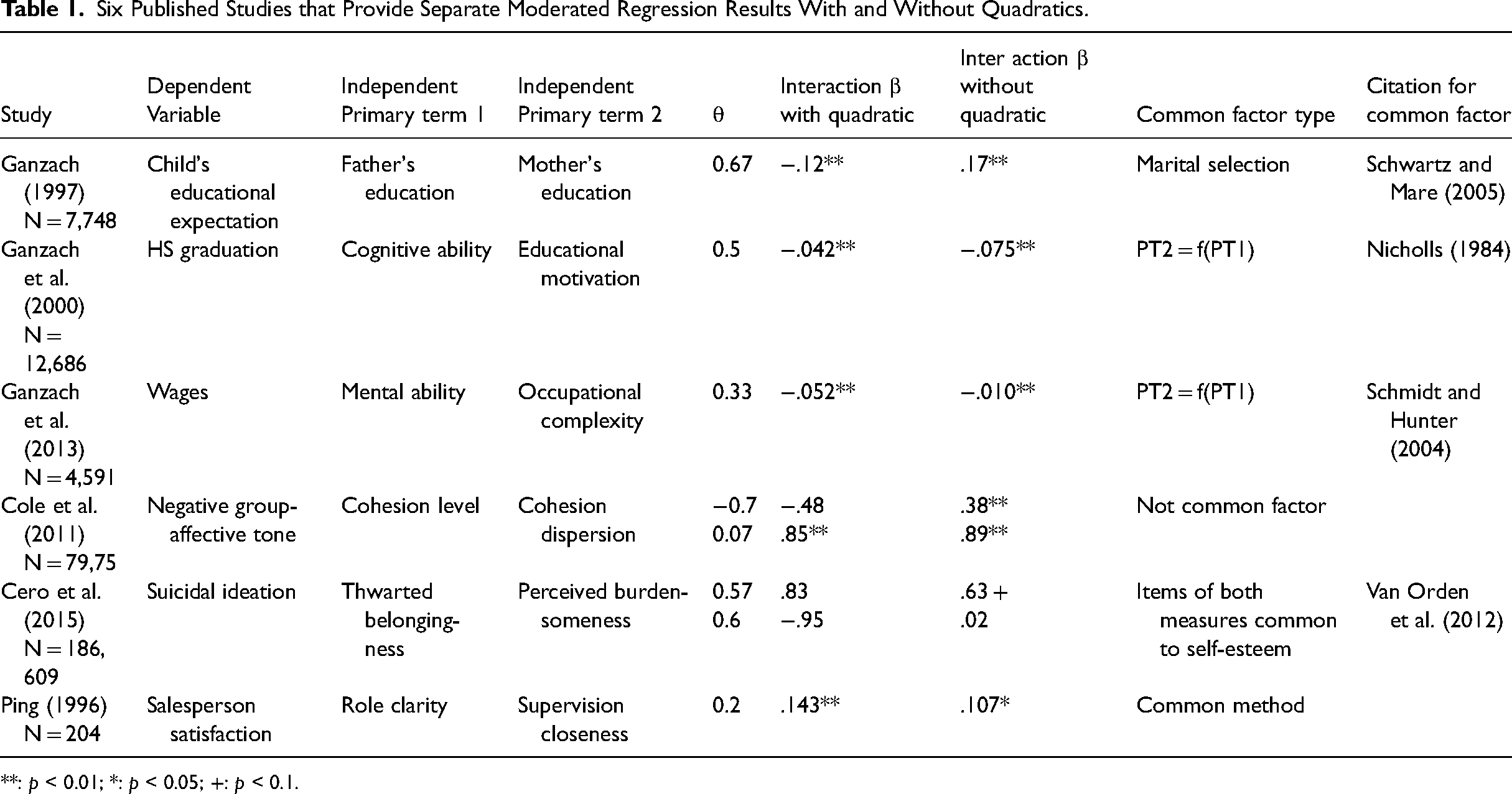
**: p < 0.01; *: p < 0.05; +: p < 0.1.

In two papers, the one primary term that is a partial cause of the other primary term is the common factor. First, in Ganzach et al. (2000), the Common Factor DGP might be the appropriate data structure because cognitive ability is a cause of educational motivation (e.g., Nicholls, 1984). Second, in Ganzach et al. (2013), the Common Factor DGP may be present because the same cognitive ability is a cause of occupational complexity (e.g., Schmidt & Hunter, 2004). The idiosyncratic components that would increase the likelihood of a Common Factor DGP are possible in these two data sets, but we would have to identify specific omitted variables that are correlated with motivation and complexity, respectively, but that are independent of ability.

In Cole et al. (2011) the primary terms cohesion dispersion and cohesion level do not have a common factor of the structure presented here. However, the combination of a linear term of level (within-group means), and a dispersion (within-group standard deviation term) of the same underlying variable may result a process similar to the structural form of the Common Factor DGP that is at work when the correlation is high, as per Cole et al.’s (2011) first analysis.

Cero et al.’s (2015) common factor may arise from the relationship between items within two multi-item measures of constructs: thwarted belongingness and perceived burdensomeness. Methodological research on these two scales using young adults has found a lack of discriminant validity: individual items within the scales have substantial commonalities with those regarding self-esteem, which may thus serve as a common factor (Van Orden et al., 2012). The idiosyncratic term here could be any item from either scale that (i) has its own quadratic effect on the DV and (ii) has no equivalent in the other scale.

Finally, Ping (1996) regressed overall salesperson satisfaction on the primary terms of role clarity and closeness of supervision. He formed each scale using five items. The items for all variables were on the same survey, thus any common method effect serves as a common factor. Any relevant, omitted variable could then serve as an idiosyncratic component.

In the next section, we present a mathematical analysis that derives the connections between the Common Factor DGP, beta polarization, and type 1 interaction errors. The practically minded reader can skip this section without loss of continuity and may proceed to the section titled “Five Questions That Determine Whether to Include Quadratics.”

A Linear Algebraic Analysis of OLS/MMR with Common Factor DGP

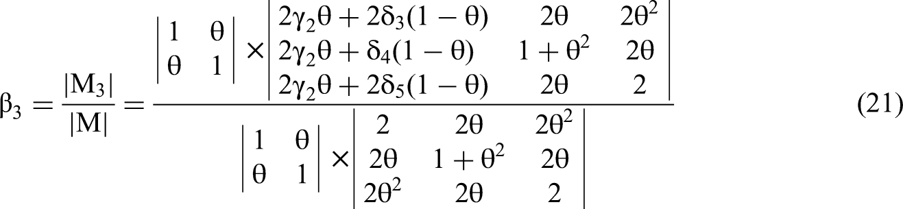
Use of Cramer's Rule to Derive Expected Values of Estimated Beta Coefficients

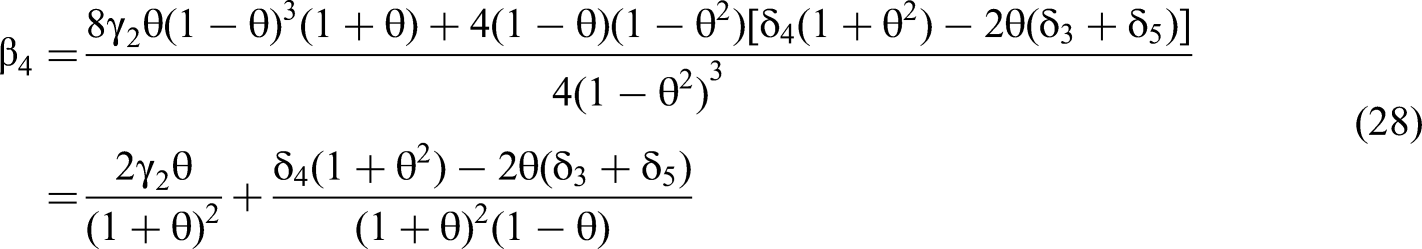
The exact values of beta coefficients estimated by any OLS regression can be derived via Cramer's Rule (e.g., Klein & Nakamura, 1962) from a covariance matrix of all variables used in the regression. We use Cramer's Rule not to derive exact numerical values but to derive expected values based on independent variables assumed only to conform to specific probability distributions. The Cramer's Rule formula for each estimated regression coefficient is a fraction based on covariance matrix determinants: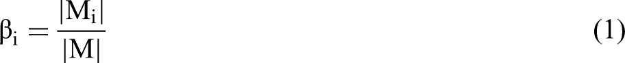

$${\beta }_{\mathrm{i}}={\displaystyle \frac{|{\mathrm{M}}_{\mathrm{i}}|}{|\mathrm{M}|}}$$

(1)

where M is the covariance matrix of all the independent variables in the regression. |M| is the determinant of M. In the case of this paper, we are investigating quadratic and interaction terms of two correlated primary variables x₁ and x₂. The M matrix is the covariance matrix of two primary (first order) and three second-order variables: x₁, x₂, x₁², x₁x₂, and x₂². The matrix M_i is matrix M with column i switched out in favor of covariances of dependent variable y with the five independent variables. Row i from M is otherwise left intact.

Because the results from the Canonical DGP are well-understood in general, if not analytically proven for this particular specification, we leave a formal proof to Appendix 1. Here we focus on the Common Factor DGP. However, the denominator of Equation 1, |M|, is identical for both DGPs because the observable and available variables x₁, x₂, x₁², x₁x₂, and x₂² remain the same in both. The dependent variable created by either DGP does not determine any part of their distributions or realized values.

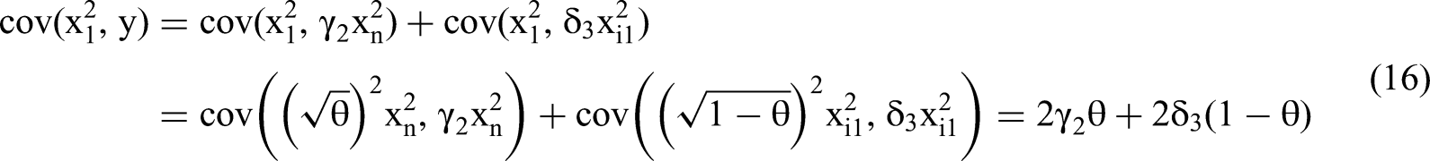
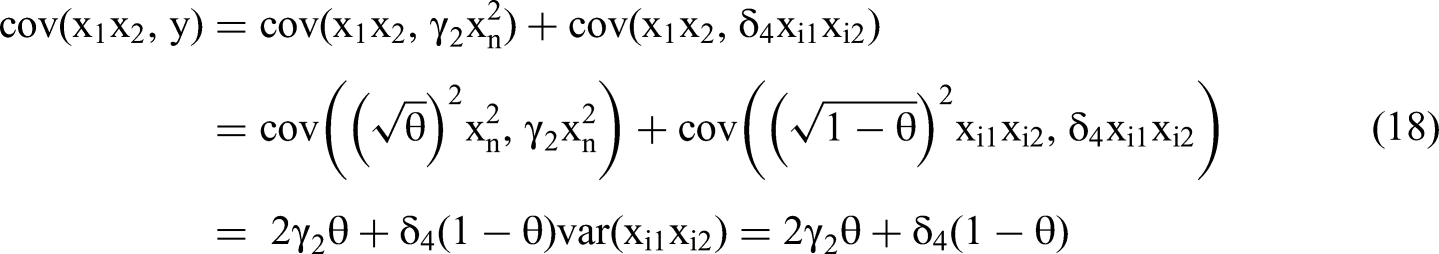
We derive all necessary variances and covariances from M that we will use to calculate |M|. We focus first on the variances. We assume x₁ and x₂ are standard normal, and thus symmetric with mean zero and variance one. The variances of x₁² and x₂² equal two as a result. The distribution of the product of two correlated normal variables such as interaction term x₁x₂ does not have a closed-form expression but the variance can be derived as a special case from Bohrnstedt and Goldberger (1969: Equation 6). ³ For the variance of a product of two distributions, the first three terms (the top row) are all zero for the product x₁x₂ because the components x₁ and x₂ are both standard normal. The variance of both components is one, and therefore the fourth term equals one. The fifth term equals θ² because cov (x₁,x₂) = θ. Therefore var (x₁x₂) = 1 + θ².

Regarding covariances, the standard normal assumption implies cov(x₁, x₁²) = 0, cov(x₂, x₂²) = 0, cov(x₁, x₁x₂) = 0 and cov(x₂, x₁x₂) = 0. The zero covariances simplify the analysis but do not inhibit generalization, because all independent variables can be standardized with no change in OLS/MMR t-statistics. The covariances of the quadratic and interaction terms are not zero. We can derive them by applying Bohrnstedt and Goldberger’s (1969) Equation 13. 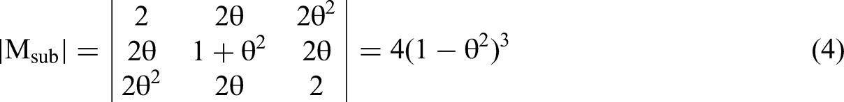⁴ First, to derive cov(x₁², x₂²), substitute both x and y with x₁, and both u and v with x₂. The first four terms are zero and the final two are equal to (cov(x₁, x₂))². Thus, cov(x₁², x₂²) = 2θ². To derive cov(x₁², x₁x₂), substitute x, y, and u with x₁, and v with x₂. The first four terms are zero and the last two equal cov(x₁, x₂). Thus, cov(x₂², x₁x₂) = 2θ. We fill M with these terms and determine |M|, which we can split into two multiplicative components due to its block diagonal structure.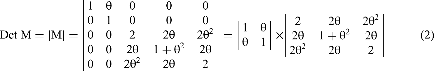

$$\mathrm{Det}\mathrm{M}=|\mathrm{M}|=\left|\begin{array}{ccccc}1& \theta & 0& 0& 0\\ \theta & 1& 0& 0& 0\\ 0& 0& 2& 2\theta & 2{\theta }^2\\ 0& 0& 2\theta & 1+{\theta }^2& 2\theta \\ 0& 0& 2{\theta }^2& 2\theta & 2\end{array}\right|=\left|\begin{array}{cc}1& \theta \\ \theta & 1\end{array}\right|\times \left|\begin{array}{ccc}2& 2\theta & 2{\theta }^2\\ 2\theta & 1+{\theta }^2& 2\theta \\ 2{\theta }^2& 2\theta & 2\end{array}\right|$$

(2)

The determinant of any 3 × 3 matrix A can be calculated in terms of its diagonal products.

$$\left|\begin{array}{ccc}{\mathrm{a}}_{11}& {\mathrm{a}}_{12}& {\mathrm{a}}_{13}\\ {\mathrm{a}}_{21}& {\mathrm{a}}_{22}& {\mathrm{a}}_{23}\\ {\mathrm{a}}_{31}& {\mathrm{a}}_{32}& {\mathrm{a}}_{33}\end{array}\right|={\mathrm{a}}_{11}{\mathrm{a}}_{22}{\mathrm{a}}_{33}+{\mathrm{a}}_{12}{\mathrm{a}}_{23}{\mathrm{a}}_{31}+{\mathrm{a}}_{13}{\mathrm{a}}_{21}{\mathrm{a}}_{32}-{\mathrm{a}}_{13}{\mathrm{a}}_{22}{\mathrm{a}}_{31}-{\mathrm{a}}_{12}{\mathrm{a}}_{21}{\mathrm{a}}_{33}-{\mathrm{a}}_{11}{\mathrm{a}}_{23}{\mathrm{a}}_{32}$$

(3)

The determinant |M_sub| of the 3 × 3 submatrix containing variances and covariances of the second-order terms x₁², x₁x₂, and x₂² can be restated based on Equation 3 as:

$$|{\mathrm{M}}_{\mathrm{sub}}|=\left|\begin{array}{ccc}2& 2\theta & 2{\theta }^2\\ 2\theta & 1+{\theta }^2& 2\theta \\ 2{\theta }^2& 2\theta & 2\end{array}\right|=4(1-{\theta }^2{)}^3$$

(4)

This determinant is the denominator in the derivations of the estimated β₃ and β₄ below.

Derivation of Expected Values of Estimated Beta Coefficients from a Common Factor DGP

In this section, we follow the analytical approach used by Kalnins (2018) for a two-variable regression and extend it to a full second-order polynomial with quadratic terms and an interaction term. The first task is to identify all the variances and covariances of the elements of M_i, column i of Equation 1, to derive each estimated β coefficient. The primary variables x₁ and x₂ are correlated only via common factor x_n. The variables x₁ and x₂ have idiosyncratic components, x_i1 and x_i2, respectively, that are independent of each other and of x_n. These idiosyncratic components are substantive omitted variables, not error terms. The variable x_n may be either a substantive common factor or a common source of measurement error. At least one idiosyncratic term must not be available to the researcher; if all the components are observable and available then researchers should include them directly in the regression, and it becomes equivalent to the Canonical DGP. We can write:

$${\mathrm{x}}_1=\mathrm{a}{\mathrm{x}}_{\mathrm{n}}+\mathrm{c}{\mathrm{x}}_{\mathrm{i}1};{\mathrm{x}}_2=\mathrm{a}{\mathrm{x}}_{\mathrm{n}}+\mathrm{c}{\mathrm{x}}_{\mathrm{i}2}$$

(5,6)

where x_i1, x_i2, and x_n represent Pearson’s (1920: 27) “uncorrelated causes” of dependent variable y. The additive form using constants a and c represents his “unknown functional relations.”

If we wish to depict the form of common factor where one independent variable is in part a function of the other, we can replace Equation 6 with x₂ = x_n. While specifics will change in the analysis below, all conclusions will remain valid.

If we assume that x_i1, x_i2, and x_n are normally distributed with mean zero, then x₁ and x₂ will also have those same characteristics. But we would like x₁ and x₂ to be standard normal because it simplifies the diagonal elements of the matrix M_sub as depicted in Equation 4. And we would like to express the Pearson correlation coefficient strictly in terms of a and c. Therefore, we must transform the x variables by, first, scaling a and c so that a + c = 1. We then take the square root of each factor's coefficient. Pearson (1920) discusses favorable properties of this scaling. The general conclusions derivable from Equations 7 and 8 are no different from Equations 5 and 6 with no transformation; they are merely more straightforward to derive and present.

$${\mathrm{x}}_1=\sqrt{{\displaystyle \frac{\mathrm{a}}{\mathrm{a}+\mathrm{c}}}}{\mathrm{x}}_{\mathrm{n}}+\sqrt{{\displaystyle \frac{\mathrm{c}}{\mathrm{a}+\mathrm{c}}}}{\mathrm{x}}_{\mathrm{i}1};{\mathrm{x}}_2=\sqrt{{\displaystyle \frac{\mathrm{a}}{\mathrm{a}+\mathrm{c}}}}{\mathrm{x}}_{\mathrm{n}}+\sqrt{{\displaystyle \frac{\mathrm{c}}{\mathrm{a}+\mathrm{c}}}}{\mathrm{x}}_{\mathrm{i}2}$$

(7,8)

Variables x₁ and x₂ will be standard normally distributed for any values of a and c and Pearson's correlation coefficient will equal $\mathrm{a}/\mathrm{a}+\mathrm{c}$ . The standard normal claim is true because, due to the independence of x_i1, x_i2, and x_n and due to their variance of one:

$$\mathrm{var}({\mathrm{x}}_1)=\mathrm{var}\left(\sqrt{{\displaystyle \frac{\mathrm{a}}{\mathrm{a}+\mathrm{c}}}}{\mathrm{x}}_{\mathrm{n}}\right)+\mathrm{var}\left(\sqrt{{\displaystyle \frac{\mathrm{c}}{\mathrm{a}+\mathrm{c}}}}{\mathrm{x}}_{\mathrm{i}1}\right)={\left(\sqrt{{\displaystyle \frac{\mathrm{a}}{\mathrm{a}+\mathrm{c}}}}\right)}^2+{\left(\sqrt{{\displaystyle \frac{\mathrm{c}}{\mathrm{a}+\mathrm{c}}}}\right)}^2=1$$

(9)

The correlation coefficient claim is true because:

$$\mathrm{cov}({\mathrm{x}}_1,{\mathrm{x}}_2)=\mathrm{cov}\left(\sqrt{{\displaystyle \frac{\mathrm{a}}{\mathrm{a}+\mathrm{c}}}}{\mathrm{x}}_{\mathrm{n}},\sqrt{{\displaystyle \frac{\mathrm{a}}{\mathrm{a}+\mathrm{c}}}}{\mathrm{x}}_{\mathrm{n}}\right)=\mathrm{var}\left(\sqrt{{\displaystyle \frac{\mathrm{a}}{\mathrm{a}+\mathrm{c}}}}{\mathrm{x}}_{\mathrm{n}}\right)={\left(\sqrt{{\displaystyle \frac{\mathrm{a}}{\mathrm{a}+\mathrm{c}}}}\right)}^2={\displaystyle \frac{\mathrm{a}}{\mathrm{a}+\mathrm{c}}}$$

(10)

While a and c must necessarily be positive for the transformation to be feasible, we can analyze negative correlations by replacing x_n with −x_n for either x₁ or x₂. We replace $\mathrm{a}/\mathrm{a}+\mathrm{c}$ with θ for expositional convenience. The system of equations is now:

$${\mathrm{x}}_1=\sqrt{\theta }{\mathrm{x}}_{\mathrm{n}}+\sqrt{1-\theta }{\mathrm{x}}_{\mathrm{i}1};{\mathrm{x}}_2=\sqrt{\theta }{\mathrm{x}}_{\mathrm{n}}+\sqrt{1-\theta }{\mathrm{x}}_{\mathrm{i}2}$$

(11,12)

We can write a very general second-order polynomial Common Factor DGP as follows:

$$\mathrm{y}={\gamma }_1{\mathrm{x}}_{\mathrm{n}}+{\gamma }_2{\mathrm{x}}_{\mathrm{n}}^2+{\delta }_1{\mathrm{x}}_{\mathrm{i}1}+{\delta }_2{\mathrm{x}}_{\mathrm{i}2}+{\delta }_3{\mathrm{x}}_{\mathrm{i}1}^2+{\delta }_4{\mathrm{x}}_{\mathrm{i}1}{\mathrm{x}}_{\mathrm{i}2}+{\delta }_5{\mathrm{x}}_{\mathrm{i}2}^2+\mathrm{e}$$

(13)

The dependent variable y of Equation 13 is a linear function of Pearson’s (1920) “uncorrelated causes,” that is, the common factor and the idiosyncratic terms, their quadratic and interaction terms, and a normally distributed error term e with mean zero. The δ values represent the true effect sizes of the independent x variables.

Note that the formulation of Equation 13 eliminates the “effect independence” assumption of the Canonical DGP that is mentioned above because the effect of the common factor is separated from those of the idiosyncratic terms.

We now populate matrix M_i, column i, with a column vector of relevant covariances that we derive below. Based on the independent, standardized structure of x_i1, x_i2 and x_n and the additive structure of the DGP for y, we know that cov(x_ij, x_ij²) = 0 and cov(x_ij, x_i1x_i2) = 0 where j = 1, 2. This simplifies the derivation. We require an assumption of normality only where noted.

$$\begin{array}{rl}\mathrm{cov}({\mathrm{x}}_1,\mathrm{y})& =\mathrm{cov}({\mathrm{x}}_1,{\gamma }_1{\mathrm{x}}_{\mathrm{n}})+\mathrm{cov}({\mathrm{x}}_1,{\delta }_1{\mathrm{x}}_{\mathrm{i}1})\\ & =\mathrm{cov}\left(\sqrt{\theta }{\mathrm{x}}_{\mathrm{n}},{\gamma }_1{\mathrm{x}}_{\mathrm{n}}\right)+\mathrm{cov}\left(\sqrt{1-\theta }{\mathrm{x}}_{\mathrm{i}1},{\delta }_1{\mathrm{x}}_{\mathrm{i}1}\right)={\gamma }_1\sqrt{\theta }+{\delta }_1\sqrt{1-\theta }\end{array}$$

(14)

$$\mathrm{cov}({\mathrm{x}}_2,\mathrm{y})={\gamma }_1\sqrt{\theta }+{\delta }_2\sqrt{1-\theta }(15)$$

(15)

$$\begin{array}{rl}\mathrm{cov}({\mathrm{x}}_1^2,\mathrm{y})& =\mathrm{cov}({\mathrm{x}}_1^2,{\gamma }_2{\mathrm{x}}_{\mathrm{n}}^2)+\mathrm{cov}({\mathrm{x}}_1^2,{\delta }_3{\mathrm{x}}_{\mathrm{i}1}^2)\\ & =\mathrm{cov}\left({\left(\sqrt{\theta }\right)}^2{\mathrm{x}}_{\mathrm{n}}^2,{\gamma }_2{\mathrm{x}}_{\mathrm{n}}^2\right)+\mathrm{cov}\left({\left(\sqrt{1-\theta }\right)}^2{\mathrm{x}}_{\mathrm{i}1}^2,{\delta }_3{\mathrm{x}}_{\mathrm{i}1}^2\right)=2{\gamma }_2\theta +2{\delta }_3(1-\theta )\end{array}$$

(16)

$$\mathrm{cov}({\mathrm{x}}_2^2,\mathrm{y})=2{\gamma }_2\theta +2{\delta }_5(1-\theta )(17)$$

(17)

The distribution of the product of two correlated standard normal variables such as interaction term x₁x₂ does not have a closed-form mathematical expression but we can derive the variance as a special case from Bohrnstedt and Goldberger (1969: Equation 6). In that equation for a variance of a product of two distributions, the first three terms (the top row) are all zero for the product x₁x₂ because the components are both standard normal, and thus each has an expectation (mean) of zero. The variance of both components is one, and therefore the fourth term equals one: var (x₁x₂) = 1 + (cov(x_1, x₂))². Because cov(x_i1, x_i2) = 0, var(x_i1x_i2) = 1. We apply this result in the derivation of Equation 18:

$$\begin{array}{rl}\mathrm{cov}({\mathrm{x}}_1{\mathrm{x}}_2,\mathrm{y})& =\mathrm{cov}({\mathrm{x}}_1{\mathrm{x}}_2,{\gamma }_2{\mathrm{x}}_{\mathrm{n}}^2)+\mathrm{cov}({\mathrm{x}}_1{\mathrm{x}}_2,{\delta }_4{\mathrm{x}}_{\mathrm{i}1}{\mathrm{x}}_{\mathrm{i}2})\\ & =\mathrm{cov}\left({\left(\sqrt{\theta }\right)}^2{\mathrm{x}}_{\mathrm{n}}^2,{\gamma }_2{\mathrm{x}}_{\mathrm{n}}^2\right)+\mathrm{cov}\left({\left(\sqrt{1-\theta }\right)}^2{\mathrm{x}}_{\mathrm{i}1}{\mathrm{x}}_{\mathrm{i}2},{\delta }_4{\mathrm{x}}_{\mathrm{i}1}{\mathrm{x}}_{\mathrm{i}2}\right)\\ & =2{\gamma }_2\theta +{\delta }_4(1-\theta )\mathrm{var}({\mathrm{x}}_{\mathrm{i}1}{\mathrm{x}}_{\mathrm{i}2})=2{\gamma }_2\theta +{\delta }_4(1-\theta )\end{array}$$

(18)

Solving for the coefficients of the quadratic terms

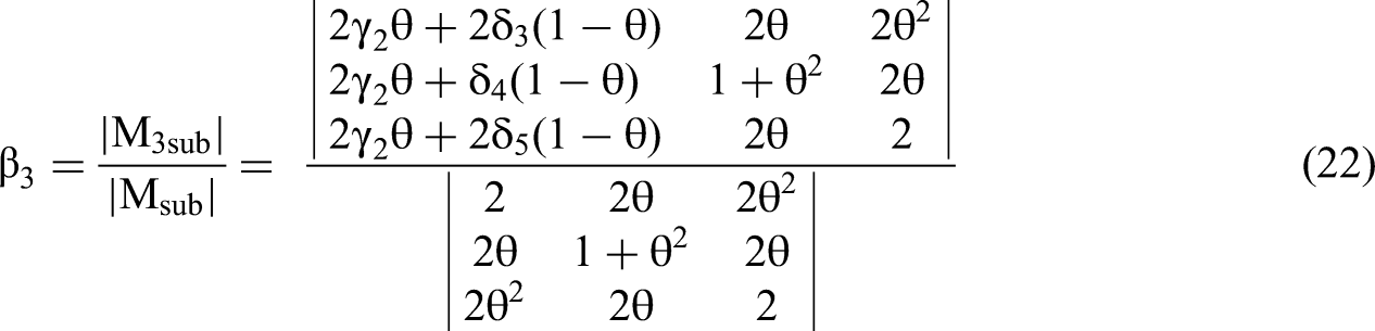
We construct a column vector using these five covariances to replace a column of matrix M. The determinants of modified matrix M_i become the numerators for Equation 1 and will allow us to solve for β₃ and β₅.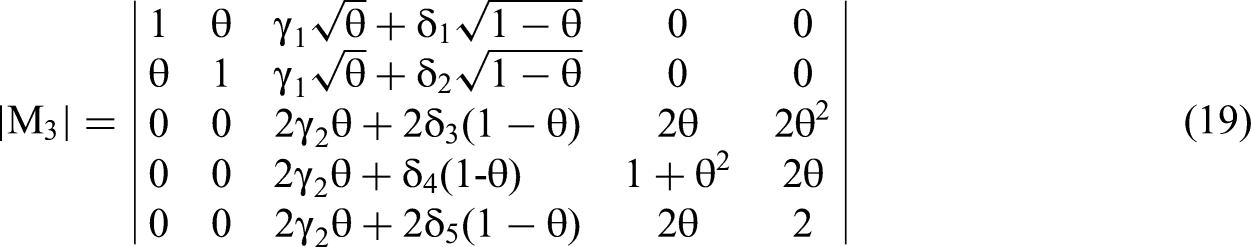

$$|{\mathrm{M}}_3|=\left|\begin{array}{ccccc}1& \theta & {\gamma }_1\sqrt{\theta }+{\delta }_1\sqrt{1-\theta }& 0& 0\\ \theta & 1& {\gamma }_1\sqrt{\theta }+{\delta }_2\sqrt{1-\theta }& 0& 0\\ 0& 0& 2{\gamma }_2\theta +2{\delta }_3(1-\theta )& 2\theta & 2{\theta }^2\\ 0& 0& 2{\gamma }_2\theta +{\delta }_4(1-\theta )& 1+{\theta }^2& 2\theta \\ 0& 0& 2{\gamma }_2\theta +2{\delta }_5(1-\theta )& 2\theta & 2\end{array}\right|$$

(19)

This square matrix is upper triangular block diagonal, that is, it takes the form M =  $\left[\begin{array}{cc}A& C\\ 0& B\end{array}\right]$ where A (2 × 2) and B (3 × 3) must be square. When there is a rectangular or square block of zeros in the lower left corner, we can ignore the zero block and C when calculating the determinant. As per Grossman (2016), det(M) = det(A) × det(B) in this case, and we can write:

$$|{\mathrm{M}}_3|=\left|\begin{array}{cc}1& \theta \\ \theta & 1\end{array}\right|\times \left|\begin{array}{ccc}2{\gamma }_2\theta +2{\delta }_3(1-\theta )& 2\theta & 2{\theta }^2\\ 2{\gamma }_2\theta +{\delta }_4(1-\theta )& 1+{\theta }^2& 2\theta \\ 2{\gamma }_2\theta +2{\delta }_5(1-\theta )& 2\theta & 2\end{array}\right|$$

(20)

Inserting this determinant into the numerator of Equation 1 yields the expected value of the estimated coefficient β₃. The coefficient is independent of the true effects δ₁ and δ₂ of primary terms x₁ and x₂ because their submatrix drops out of the equation. However, the estimated coefficient β₃ will remain a function of not only δ₃, the true effect of x₁², but also of δ₄ and δ₅, the true effects of variables x₁x₂ and x₂². This provides intuition regarding why the estimated β coefficient values may be far different from their true δ values and why type 1 errors may occur.

$${\beta }_3={\displaystyle \frac{|{\mathrm{M}}_3|}{|\mathrm{M}|}={\displaystyle \frac{\left|\begin{array}{cc}1& \theta \\ \theta & 1\end{array}\right|\times \left|\begin{array}{ccc}2{\gamma }_2\theta +2{\delta }_3(1-\theta )& 2\theta & 2{\theta }^2\\ 2{\gamma }_2\theta +{\delta }_4(1-\theta )& 1+{\theta }^2& 2\theta \\ 2{\gamma }_2\theta +2{\delta }_5(1-\theta )& 2\theta & 2\end{array}\right|}{\left|\begin{array}{cc}1& \theta \\ \theta & 1\end{array}\right|\times \left|\begin{array}{ccc}2& 2\theta & 2{\theta }^2\\ 2\theta & 1+{\theta }^2& 2\theta \\ 2{\theta }^2& 2\theta & 2\end{array}\right|}}}$$

(21)

We can rewrite this fraction more simply because the primary term sub-matrices cancel:

$${\beta }_3={\displaystyle \frac{|{\mathrm{M}}_{3\mathrm{sub}}|}{|{\mathrm{M}}_{\mathrm{sub}}|}={\displaystyle \frac{\left|\begin{array}{ccc}2{\gamma }_2\theta +2{\delta }_3(1-\theta )& 2\theta & 2{\theta }^2\\ 2{\gamma }_2\theta +{\delta }_4(1-\theta )& 1+{\theta }^2& 2\theta \\ 2{\gamma }_2\theta +2{\delta }_5(1-\theta )& 2\theta & 2\end{array}\right|}{\left|\begin{array}{ccc}2& 2\theta & 2{\theta }^2\\ 2\theta & 1+{\theta }^2& 2\theta \\ 2{\theta }^2& 2\theta & 2\end{array}\right|}}}$$

(22)

Before continuing with the analysis, we state the first conclusion, based on Equation 22. This conclusion is important for the derivation of the standard errors below:

Conclusion 1:

True primary term effects δ₁ and δ₂ will not influence estimated quadratic or interaction coefficients β₃, β₄, β₅.

This conclusion is consistent with the known fact that interaction term coefficient estimates such as β₄, regardless of distributional assumptions, will never change due to primary term re-scaling (Aiken & West, 1991). Edwards (2009) adds insight by stating in his Myth #1 that even in non-normal, non-symmetric cases any variable x can be re-scaled such that the resulting covariances of primary terms with interaction terms are equal to zero, even if this scaling is not necessarily mean-centering as is the case here. This suggests that a particular scaling exists that will make the M and M_i matrices upper triangular block diagonal for any regression and DGP. We leave a rigorous proof for future work.

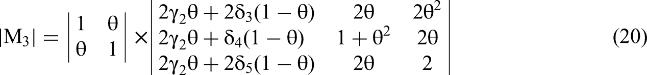
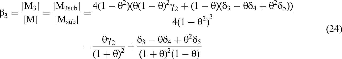
Returning to the analysis, we use Equation 3 to solve the numerator of the β₃ equation based on Cramer's Rule, the determinant of M_3sub: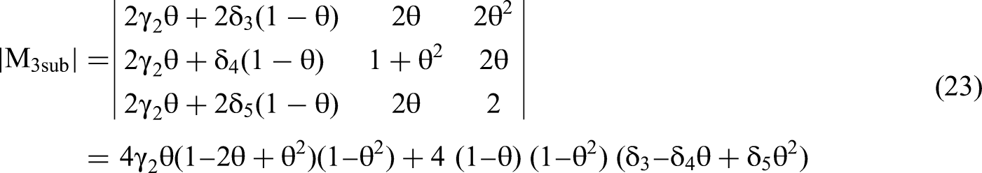

$$\begin{array}{rl}|{\mathrm{M}}_{3\mathrm{sub}}|& =\left|\begin{array}{ccc}2{\gamma }_2\theta +2{\delta }_3(1-\theta )& 2\theta & 2{\theta }^2\\ 2{\gamma }_2\theta +{\delta }_4(1-\theta )& 1+{\theta }^2& 2\theta \\ 2{\gamma }_2\theta +2{\delta }_5(1-\theta )& 2\theta & 2\end{array}\right|\\ & =4{\gamma }_2\theta (1\text{–}2\theta +{\theta }^2)(1\text{–}{\theta }^2)+4(1\text{–}\theta )(1\text{–}{\theta }^2)({\delta }_3\text{–}{\delta }_4\theta +{\delta }_5{\theta }^2)\end{array}$$

(23)

This determinant value becomes the numerator of the Cramer's Rule fraction of Equation 1. We calculated the denominator |M_sub| earlier in Equation 4.

$$\begin{array}{rl}{\beta }_3={\displaystyle \frac{|{\mathrm{M}}_3|}{|\mathrm{M}|}={\displaystyle \frac{|{\mathrm{M}}_{3\mathrm{sub}}|}{|{\mathrm{M}}_{\mathrm{sub}}|}=}}& {\displaystyle \frac{4(1-{\theta }^2)(\theta {(1-\theta )}^2{\gamma }_2+(1-\theta )({\delta }_3-\theta {\delta }_4+{\theta }^2{\delta }_5))}{4{(1-{\theta }^2)}^3}}\\ =& {\displaystyle \frac{\theta {\gamma }_2}{{(1+\theta )}^2}+{\displaystyle \frac{{\delta }_3-\theta {\delta }_4+{\theta }^2{\delta }_5}{{(1+\theta )}^2(1-\theta )}}}\end{array}$$

(24)

We obtain the equality between the two rightmost fractions by (1) dividing out 4 (1 − θ²) from numerator and denominator, (2) replacing the remaining (1 − θ²) terms with (1 − θ) (1 + θ), and (3) dividing out (1 − θ)² the first term and (1 − θ) from the second. Similarly, we can derive:

$${\beta }_5={\displaystyle \frac{\theta {\gamma }_2}{{(1+\theta )}^2}+{\displaystyle \frac{{\delta }_5-\theta {\delta }_4+{\theta }^2{\delta }_3}{{(1+\theta )}^2(1-\theta )}}}$$

(25)

To observe what will happen to the expected values of the estimated beta coefficients when the correlation θ between primary terms gets large, we take the limit as θ → 1 from the left, designated as θ → 1−. Because the correlation cannot be more than one, we need not consider the limit from the right. The variable ε represents the limit of (1 − θ) in the form of a small value closer to zero than any other value that can be named.

$$\underset{\theta \to 1-}{lim}{\beta }_3=\underset{\theta \to 1-}{lim}{\beta }_5={\displaystyle \frac{{\gamma }_2}{4}+{\displaystyle \frac{{\delta }_3-{\delta }_4+{\delta }_5}{4\epsilon }=+\mathrm{\infty }\mathrm{if}{\delta }_3+{\delta }_5>{\delta }_4;=-\mathrm{\infty }\mathrm{if}{\delta }_3+{\delta }_5<{\delta }_4}}$$

(26)

Because x₁² and x₂² both have equivalent covariances with the primary terms and the interaction term, the limit equation for β₅ will equal that of β₃ in Equation 26. Regardless of what the quadratic terms’ true effect sizes δ₃ and δ₅ are, as the correlation of the two primary variables approaches 1, OLS/MMR will always estimate β values that approach infinity and are of the same sign for both quadratic terms.

Solving for the coefficient of the interaction term

We reduce the matrix for the interaction term, M₄, to a 3 × 3 matrix, M_4sub, using the upper triangular block diagonal theorem and Conclusion 1, as we did for M₃ shown in Equation 23.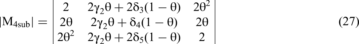

$$|{\mathrm{M}}_{4\mathrm{sub}}|=\left|\begin{array}{ccc}2& 2{\gamma }_2\theta +2{\delta }_3(1-\theta )& 2{\theta }^2\\ 2\theta & 2{\gamma }_2\theta +{\delta }_4(1-\theta )& 2\theta \\ 2{\theta }^2& 2{\gamma }_2\theta +2{\delta }_5(1-\theta )& 2\end{array}\right|$$

(27)

is the numerator for the derivation of β₄, as per Equation 1. |M_sub| remains the denominator.

$$\begin{array}{rl}{\beta }_4=& {\displaystyle \frac{8{\gamma }_2\theta {(1-\theta )}^3(1+\theta )+4(1-\theta )(1-{\theta }^2)[{\delta }_4(1+{\theta }^2)-2\theta ({\delta }_3+{\delta }_5)]}{4{(1-{\theta }^2)}^3}}\\ =& {\displaystyle \frac{2{\gamma }_2\theta }{{(1+\theta )}^2}+{\displaystyle \frac{{\delta }_4(1+{\theta }^2)-2\theta ({\delta }_3+{\delta }_5)}{{(1+\theta )}^2(1-\theta )}}}\end{array}$$

(28)

The intermediate steps to derive this equation are the same as those for Equation 24. An analysis of Equation 28 shows that the estimated value of β₄ shows bias based linearly on the size of the true quadratic effects. This observation leads to the second conclusion, which is central to establishing the generalizability of the results depicted in the figures later in the paper:

Conclusion 2:

For a given correlation θ the true quadratic effects δ₃ and δ₅ bias the estimated interaction term coefficient β₄ linearly and additively.

If the true quadratic effect δ₃ = k₁ adds bias −2θk₁/z, where z = (1 + θ)² (1 − θ), to β₄ via the last component of Equation 28, then doubling δ₃, the true quadratic effect, doubles that component's effect on the bias of β₄. This confirms linearity. If the other quadratic term's effect is δ₅ = k₂, then the bias on the interaction via the last component of Equation 28 will be −2θ(k₁ + k₂)/z. If only one of the quadratic terms has a true effect size δ₃ = k₁ + k₂, the component's contribution to the bias will still be −2θ(k₁ + k₂)/z. This confirms the additivity claim of Conclusion 2.

We now consider the case of the estimated β₄ coefficient's expected value when the correlation θ between primary terms approaches 1. We can write the value of β₄ in the limit as:

$$\underset{\theta \to 1-}{lim}{\beta }_4={\displaystyle \frac{{\gamma }_2}{2}+{\displaystyle \frac{{\delta }_4-{\delta }_3-{\delta }_5}{2\epsilon }=+\mathrm{\infty }\mathrm{if}{\delta }_4>{\delta }_3+{\delta }_5;=-\mathrm{\infty }\mathrm{if}{\delta }_4<{\delta }_3+{\delta }_5}}$$

(29)

As in Equation 26, ε represents a small value closer to zero than any other value. We observe that, regardless of the interaction term's true effect δ₄, as the correlation θ of the two primary variables approaches the limit of 1, OLS/MMR will always produce an estimated β₄ value that approaches infinite magnitude. Considering this result together with that of Equation 26, for β₃ and β₅, we see that the estimated β₄ value is necessarily opposite in sign from the estimated β₃ and β₅.

Conclusion 3:

We consider the case where two primary terms are correlated via a common factor, the DV is generated by the Common Factor DGP, and the correlation θ of the two primary terms approaches 1. If we include quadratic terms as controls:

(3a) The estimated coefficients of the two quadratic terms will be of the same sign and will approach positive or negative infinity regardless of their true δ values.

(3b) Beta polarization will occur. The estimated coefficient of the interaction term will be of the opposite sign to that of the quadratic terms, and will also approach an infinite absolute value, again regardless of its true δ value.

(3c) If we do not include quadratic terms in the regression, the coefficient of the interaction term will not approach positive or negative infinity regardless of the correlation of the primary terms.

Conclusion 4: If the only true effect is the quadratic γ₂ of the common factor, the effects will be distributed across β₃, β₄, and β₅. These effects however will remain small regardless of correlation θ because their denominators do not approach zero.

Negative Correlation of Primary Terms

We now extend the above analyses to the case of a negative correlation −θ between primary terms x₁ and x₂ by replacing x_n with −x_n in Equation 11 or 12, but not both. Conceptually −θ functions as an “opposing” factor instead of a common factor, but otherwise the form of the Common Factor DGP remains in effect. We cannot insert negative values for θ directly into Equations 24, 25, and 28. These equations are valid only for the positive range of θ. To derive the correct values of the estimated β for negative correlations, we must modify the determinants |M_sub|, |M_3sub|, and |M_4sub|, depicted in Equations 4, 23, and 27, respectively.

Regarding |M_sub|, the only changes to the variances or covariances among the second-order independent variables that result from flipping θ to a negative value are that cov(x₁x₂,x₁²) and cov(x₁x₂,x₂²) = −2θ instead of 2θ. Cov(x₁²,x₂²) and var(x₁x₂) keep the same values for θ and −θ. Because of this similarity, |M_sub| will also remain the same. The intuition for this equality can be gleaned from modifying any 3 × 3 matrix A^fs by flipping signs of the elements in positions (2,1); (1,2); (2,3); (3,2) and thus turning the matrix A^fs into matrix A. As per Equation 3 above: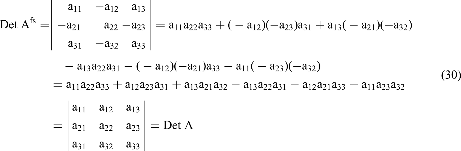

$$\begin{array}{rl}\mathrm{Det}{\mathrm{A}}^{\mathrm{fs}}=& \left|\begin{array}{ccc}{\mathrm{a}}_{11}& -{\mathrm{a}}_{12}& {\mathrm{a}}_{13}\\ -{\mathrm{a}}_{21}& {\mathrm{a}}_{22}& -{\mathrm{a}}_{23}\\ {\mathrm{a}}_{31}& -{\mathrm{a}}_{32}& {\mathrm{a}}_{33}\end{array}\right|={\mathrm{a}}_{11}{\mathrm{a}}_{22}{\mathrm{a}}_{33}+(-{\mathrm{a}}_{12})(-{\mathrm{a}}_{23}){\mathrm{a}}_{31}+{\mathrm{a}}_{13}(-{\mathrm{a}}_{21})(-{\mathrm{a}}_{32})\\ & -{\mathrm{a}}_{13}{\mathrm{a}}_{22}{\mathrm{a}}_{31}-(-{\mathrm{a}}_{12})(-{\mathrm{a}}_{21}){\mathrm{a}}_{33}-{\mathrm{a}}_{11}(-{\mathrm{a}}_{23})(-{\mathrm{a}}_{32})\\ & ={\mathrm{a}}_{11}{\mathrm{a}}_{22}{\mathrm{a}}_{33}+{\mathrm{a}}_{12}{\mathrm{a}}_{23}{\mathrm{a}}_{31}+{\mathrm{a}}_{13}{\mathrm{a}}_{21}{\mathrm{a}}_{32}-{\mathrm{a}}_{13}{\mathrm{a}}_{22}{\mathrm{a}}_{31}-{\mathrm{a}}_{12}{\mathrm{a}}_{21}{\mathrm{a}}_{33}-{\mathrm{a}}_{11}{\mathrm{a}}_{23}{\mathrm{a}}_{32}\\ & =\left|\begin{array}{ccc}{\mathrm{a}}_{11}& {\mathrm{a}}_{12}& {\mathrm{a}}_{13}\\ {\mathrm{a}}_{21}& {\mathrm{a}}_{22}& {\mathrm{a}}_{23}\\ {\mathrm{a}}_{31}& {\mathrm{a}}_{32}& {\mathrm{a}}_{33}\end{array}\right|=\mathrm{Det}\mathrm{A}\end{array}$$

(30)

Now consider the case of matrix M^fs_sub of Equation 4 where the value −2θ appears in place of 2θ in positions (2,1); (1,2); (2,3); (3,2). All diagonal products of M^fs_sub will have a factor of (–2θ)², which equals (2θ)², so the determinant of M^fs_sub will equal that of M_sub.

The numerators of Equation 1 as depicted in Equations 23 and 27 will have determinants that are necessarily of opposite sign when the primary term correlation is −θ instead of θ. First, for the case of β₄, in Equation 27, we must use the absolute value |θ| and (1 − |θ|), in place of θ and (1 − θ), in the second column of the matrix. The multipliers of the δ terms must remain between zero and one, not between one and two. Second, there are two instances of 2θ in M_sub4 that will flip to −2θ, in positions (2,1) and (2,3) of the matrix. Four of the six diagonal products contain one instance of 2θ that flips to −2θ; all these products also contain a single linear instance of either δ₃ or δ₅, but not both, and no instances of δ₄. Nothing flips sign in the two diagonals with an instance of δ₄. Therefore, the contribution of δ₃ and δ₅ in the derivation of β₄ will be of equal magnitude but opposite in sign to that of Equation 27. The γ₂ effect may also change but that is irrelevant to the value in the limit from the right, where the γ₂ effect disappears. Equation 31 presents an adaptation of Equation 29 for a negative correlation −θ. We designate the limit from the right by a + sign after the −1.

$$\underset{\theta \to -1+}{lim}{\beta }_4={\displaystyle \frac{{\gamma }_2}{2}+{\displaystyle \frac{{\delta }_4+{\delta }_3+{\delta }_5}{2|\epsilon |}=+\mathrm{\infty }\mathrm{if}{\delta }_4+{\delta }_3+{\delta }_5>0;=-\mathrm{\infty }\mathrm{if}{\delta }_4+{\delta }_3+{\delta }_5<0}}$$

(31)

The variable |ε| represents the limit of (1 − |θ|) in the form of a small absolute value closer to zero than any other value.

For the case of β₃, from Equation 23, there are three instances of 2θ in M_sub3, that flip to −2θ, in positions (1,2), (3,2) and (2,1) of the matrix. As a result, two of the six diagonal products contain two instances each of 2θ that flip to −2θ; two diagonal products contain no such instances; all four of these products also contain a single linear instance of either δ₃ or δ₅, but not both, and no instances of δ₄. Because (–2θ)² equals (2θ)², the effects of δ₃ or δ₅ on β₃ will neither flip signs nor change their magnitudes. The sign will flip only in the two diagonals that have instances of δ₄ and a single instance of 2θ that flips to −2θ. The interaction's true effect size δ₄ in the calculation of β₃ will be of equal magnitude but opposite sign to that in Equation 26, when the primary term correlation is negative. The γ₂ effect will change but that has no effect on the value in the limit. Because x₁² and x₂² both have equivalent covariances with all terms, the same result holds for β₃ and β₅. We define the variable |ε| as per Equation 31 above.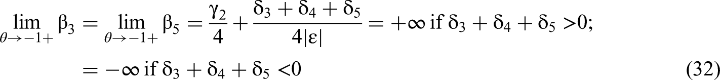

$$\underset{\theta \to -1+}{lim}{\beta }_3=\underset{\theta \to -1+}{lim}{\beta }_5={\displaystyle \frac{{\gamma }_2}{4}+{\displaystyle \frac{{\delta }_3+{\delta }_4+{\delta }_5}{4|\epsilon |}=+\mathrm{\infty }\mathrm{if}{\delta }_3+{\delta }_4+{\delta }_5>0;=-\mathrm{\infty }\mathrm{if}{\delta }_3+{\delta }_4+{\delta }_5<0}}$$

(32)

Conclusion 5:

Consider the case where two primary terms are correlated, negatively, via an opposing factor, and the DV is otherwise generated identically to the Common Factor DGP. If we include quadratic terms as controls, then, as the correlation θ of the two primary variables approaches −1:

(5a) Conclusions 3a, 3c, and 4 will apply identically for the opposing factor case as for the common factor case with + θ correlation.

(5b) Beta homogenization will occur, the opposite of beta polarization. The estimated coefficient of the interaction term will always be of the same sign to that of the quadratic terms, and all three will approach an infinite absolute value, regardless of true values.

Deriving Standard Error and t-statistic for an Expected Value of the Estimated β₄

To determine the likelihood that an estimated non-zero β₄ will appear as a type 1 error in the full second-order polynomial regression, if the true value of δ₄ is zero, we must derive the value of its standard error in terms of the true values of the second-order polynomial variable effects, δ₃ and δ₅, and the primary term correlation θ. A confidence interval for β₄ can then be determined via the t-statistic that divides the expected value of the estimate of β₄ by its standard error. The likelihood that the confidence interval does not include zero is equivalent to the likelihood of obtaining a type 1 error, because the true value of δ₄ is zero. We provide examples following the derivation.

Once we have obtained the expected β coefficients in terms of the true δ values, we can derive the standard error for each β based on additional information in the covariance matrix plus the sample size N. We calculate the residual sum of squares divided by N as follows:

$${\displaystyle \frac{\mathrm{RSS}}{\mathrm{N}}=\mathrm{var}(\mathrm{y})-\sum _{\mathrm{i}}{\beta }_{\mathrm{i}}^2\mathrm{Var}({\mathrm{X}}_{\mathrm{i}})-\sum _{\mathrm{i}\ne \mathrm{j}}2{\beta }_{\mathrm{i}}{\beta }_{\mathrm{j}}\mathrm{Cov}({\mathrm{X}}_{\mathrm{i}}{\mathrm{X}}_{\mathrm{j}})}$$

(33)

Var(y) is the total sum of squares divided by N, and the two sums Σ represent the explained sum of squares divided by N. We derive Equation 33 in Appendix 3. For a second-order polynomial with no direct effects of primary terms, we can rewrite Equation 33 as:

$$\begin{array}{rl}{\displaystyle \frac{\mathrm{RSS}}{\mathrm{N}}=}& \mathrm{var}(\mathrm{y})-{\beta }_3^2\mathrm{var}({\mathrm{x}}_1^2)-{\beta }_4^2\mathrm{var}({\mathrm{x}}_1{\mathrm{x}}_2)-{\beta }_5^2\mathrm{var}({\mathrm{x}}_2^2)\\ & -2{\beta }_3{\beta }_4\mathrm{cov}({\mathrm{x}}_1^2,{\mathrm{x}}_1{\mathrm{x}}_2)-2{\beta }_5{\beta }_4\mathrm{cov}({\mathrm{x}}_2^2,{\mathrm{x}}_1{\mathrm{x}}_2)-2{\beta }_3{\beta }_5\mathrm{cov}({\mathrm{x}}_1^2{,\mathrm{x}}_2^2),\end{array}$$

(34)

where the variances and covariance are those derived in Equations 14–18, and the β are the estimated coefficients calculated via Equation 1.

Based on the derivation provided in Appendix 4, we can write the standard error equation for each β_i as:

$$\mathrm{SE}({\beta }_{\mathrm{i}})=\sqrt{{\mathrm{m}}_{\mathrm{ii}}^{-1}{\displaystyle \frac{\mathrm{RSS}/\mathrm{y}}{\mathrm{N}-\mathrm{K}-1}}}$$

(35)

where element m_ii⁻¹ is associated with variable i on the diagonal of the inverse covariance matrix.

To simplify the analysis of the standard errors of the β, we limit the scope to cases of non-zero δ₃ and δ₅. First, we do not need to consider cases where γ₂ is non-zero. As per Conclusion 4, the magnitude of γ₂, the true effect of the common factor quadratic, does not play a significant role in the possibility of a type 1 error; as θ increases, γ₂'s relative effect decreases. Second, because we are interested in real quadratic effects and the likelihood that they generate type 1 interaction errors, we focus on cases where the true interaction effect δ₄ = 0, in other words, H₀ is true. Third, as per Conclusion 1, we need not consider the effects of primary terms: δ₁ and δ₂. Therefore, we can simplify the Common Factor DGP from Equation 13 as:

$$\mathrm{y}={\delta }_3{\mathrm{x}}_{\mathrm{i}1}^2+{\delta }_5{\mathrm{x}}_{\mathrm{i}2}^2+\mathrm{e}$$

(36)

Using the fact that x_i1², x_i2² and e are uncorrelated, we can derive the variance of a dependent variable generated by the specific form of the Common Factor DGP of Equation 36:

$$\mathrm{var}(\mathrm{y})={\displaystyle \frac{{\mathrm{y}}^{\mathrm{\prime }}\mathrm{y}}{\mathrm{n}}={\delta }_3^2\mathrm{var}({\mathrm{x}}_{\mathrm{i}1}^2)+{\delta }_5^2\mathrm{var}({\mathrm{x}}_{\mathrm{i}2}^2)+\mathrm{var}(\mathrm{e})={2\delta }_3^2+{2\delta }_5^2+1}$$

(37)

We begin by evaluating all the products of the β₃, β₄, and β₅ coefficients written out in terms of θ, δ₃, and δ₅, as per Equations 24, 25 and 28, respectively, and the variance-covariance matrix X′X from Equation 4. We then combine Equations 38–43 to calculate RSS/N using the format of Equation 34.

$${\beta }_3^2\mathrm{var}({\mathrm{x}}_1^2)={\displaystyle \frac{2[{\delta }_3^2+2{\theta }^2{\delta }_3{\delta }_5+{\theta }^4{\delta }_5^2]}{{[{(1+\theta )}^2(1-\theta )]}^2}}$$

(38)

$${\beta }_5^2\mathrm{var}({\mathrm{x}}_2^2)={\displaystyle \frac{2[{\delta }_5^2+2{\theta }^2{\delta }_3{\delta }_5+{\theta }^4{\delta }_3^2]}{{[{(1+\theta )}^2(1-\theta )]}^2}}$$

(39)

$${\beta }_4^2\mathrm{var}({\mathrm{x}}_1{\mathrm{x}}_2)={\displaystyle \frac{4{\theta }^2(1+{\theta }^2){({\delta }_3+{\delta }_5)}^2}{{[{(1+\theta )}^2(1-\theta )]}^2}}$$

(40)

$$2{\beta }_3{\beta }_4\mathrm{cov}({\mathrm{x}}_1^2,{\mathrm{x}}_1{\mathrm{x}}_2)={\displaystyle \frac{4\theta [-2\theta {\delta }_3({\delta }_3+{\delta }_5)-2{\theta }^3{\delta }_5({\delta }_3+{\delta }_5)]}{{[{(1+\theta )}^2(1-\theta )]}^2}}$$

(41)

$$2{\beta }_5{\beta }_4\mathrm{cov}({\mathrm{x}}_2^2,{\mathrm{x}}_1{\mathrm{x}}_2)={\displaystyle \frac{4\theta [-2\theta {\delta }_5({\delta }_3+{\delta }_5)-2{\theta }^3{\delta }_3({\delta }_3+{\delta }_5)]}{{[{(1+\theta )}^2(1-\theta )]}^2}}$$

(42)

$$2{\beta }_3{\beta }_5\mathrm{cov}({\mathrm{x}}_1^2{,\mathrm{x}}_2^2)={\displaystyle \frac{4{\theta }^2[{\theta }^2{(\delta }_3^2+{\delta }_5^2)+(1+{\theta }^4){\delta }_3{\delta }_5]}{{[{(1+\theta )}^2(1-\theta )]}^2}}$$

(43)

We simplify the denominator of all these equations as follows:

$$[{(1+\theta )}^2(1\text{–}\theta ){]}^2=[(1+\theta )(1+\theta )(1\text{–}\theta ){]}^2=[(1+\theta )(1\text{–}{\theta }^2){]}^2=(1+\theta {)}^2(1\text{–}{\theta }^2{)}^2$$

(44)

Inserting Equations 38–44 into Equation 34 and simplifying as per Appendix 5, we obtain RSS/N in terms of θ and the δ values:

$${\displaystyle \frac{\mathrm{RSS}(\delta ,\theta )}{\mathrm{N}}={\displaystyle \frac{{(1+\theta )}^2{[2\delta }_3^2+{2\delta }_5^2+1]}{{(1+\theta )}^2}\text{-}{\displaystyle \frac{2[{\delta }_3^2+{\delta }_5^2+2{\theta }^2{\delta }_3{\delta }_5]}{{(1+\theta )}^2}}}}$$

(45)

The next derivation required to evaluate the standard error in Equation 35 is the diagonal element m₂₂⁻¹ of the inverse of the M_sub matrix. Element m₂₂⁻¹ is associated with the interaction term x₁x₂ using the indexing for a 3 × 3 matrix as presented in Equation 3. As per the standard formula for the inverse element in position (2,2) of a 3 × 3 matrix we can write:

$${\mathrm{m}}_{22}^{-1}={\displaystyle \frac{{\mathrm{m}}_{11}{\mathrm{m}}_{33-}{\mathrm{m}}_{31}{\mathrm{m}}_{13}}{|{\mathrm{M}}_{\mathrm{sub}}|}={\displaystyle \frac{4(1-{\theta }^4)}{4{(1-{\theta }^2)}^3}={\displaystyle \frac{(1+{\theta }^2)}{{(1-{\theta }^2)}^2}}}}$$

(46)

where m_ii are the corner elements of M_sub as per Equation 3. We derived |M_sub| in Equation 4.

We use the expressions for RSS(θ,δ)/N and m₂₂⁻¹, as per Equations 45 and 46, to solve for the standard error of the interaction coefficient in terms of the δ's and θ via the structure of Equation 35. We then calculate the t-statistic for the estimated β₄ (Equation 28) by dividing the expected value of the estimated beta by the standard error.

$$\mathrm{SE}({\beta }_4)=\sqrt{{\displaystyle \frac{(1+{\theta }^2)({(1+\theta )}^2+{4\theta (\delta }_3^2+{\delta }_5^2)+2{\theta }^2{(\delta }_3^2+{\delta }_5^2)-4{\theta }^2{\delta }_3{\delta }_5)}{(\mathrm{N}-4){(1-{\theta }^2)}^2{(1+\theta )}^2}}}$$

(47)

$$\mathrm{t}={\displaystyle \frac{{\beta }_4}{\mathrm{SE}({\beta }_4)}=-2\theta ({\delta }_3+{\delta }_5)\sqrt{{\displaystyle \frac{(\mathrm{N}-4)}{(1+{\theta }^2)({(1+\theta )}^2+{4\theta (\delta }_3^2+{\delta }_5^2)+2{\theta }^2{(\delta }_3^2+{\delta }_5^2)-4{\theta }^2{\delta }_3{\delta }_5)}}}}$$

(48)

The Relationship Between the t-statistic and the Likelihood of a Type 1 Interaction Error

We consider the case of N-sized, Common Factor DGP samples where there are true quadratic effects but no true interaction effect, as per Equation 36. The proportion of such samples that will yield a type 1 error is the area under a normal distribution, i.e., either the Cumulative Distribution Function (CDF), or 1 − CDF, with a mean t-statistic that is further from zero than the cutoff value with a desired p-value. For example, the most common desired p-value is p < .05; the associated cutoff is ± 1.96. If the t-statistic of the estimated β₄ is ± 1.96, then the CDF equals 0.5 at the cutoff. This implies that 50% of samples of size N generated by the Common Factor DGP of Equation 36 will have a two-tailed 95% confidence interval for the estimated β₄ that does not include zero. For these, the estimated β₄ will falsely reject the null hypothesis H_o: β₄ = 0 with p < .05 even though δ₄ = 0. In other words, 50% of samples will be type 1 interaction errors, ten times the normal 5% likelihood from data generated by the Canonical DGP.

Even if the t-statistic of the expected value of the estimated β₄ is smaller in absolute value than 1.96, the proportion of samples that will yield type 1 errors may remain substantial. If the t-statistic of the expected value of the estimated β₄ is −1.11, then the CDF equals 0.20 at the cutoff of −1.96. This implies that 20% of samples of size N will have a two-tailed 95% confidence interval for the estimated β₄ that does not include zero, four times the normal 5% likelihood. If the estimated β₄ were positive, we would then be calculating the relevant value of 1 − CDF using a cutoff of positive 1.96; the conclusions would otherwise be the same.

Based on the logic of the previous paragraphs, we calculate sample-size dependent correlation “cutoffs” for type 1 interaction errors when the Common Factor DGP has generated the DV, and when δ₄ = 0. To do so, we used Equation 48 and chose a t-statistic value of −1.11, so that 20% of samples of size N will be type 1 interaction errors. Further, we assumed “small to medium” quadratic effect sizes δ₃ and δ₅, as per Cohen (1988). Our conclusions are, first, that absolute values of correlations |θ| < 0.5 are too small to generate 20% type 1 errors when N < 100. Second, if N > 100, only correlations |θ| < 0.3 are too small to generate type 1 errors for N < 1,000. Correlations 0.3 < |θ| < 0.5 may no longer be benign. Finally, only correlations |θ| < 0.2 are too small to generate type 1 errors for N < 1,000.

Beta Polarization/Homogenization when Correlations are Moderate

If a dependent variable has been generated by the Common Factor DGP, we have shown that in an extreme case of positive correlation approaching one, beta polarization will always occur. The estimated interaction term coefficient will always be of opposite sign to those of the quadratic terms, as per Conclusion 3b. In the case of negative correlation, beta homogenization will occur, as per Conclusion 4b. But what about more realistic cases such as those discussed in the previous section on t-statistics where correlations between primary terms are moderate, and below levels that methods texts consider problematic? Consider a case where the only true effect on the dependent variable is that of x_i1²: δ₃ > 0. There is no true effect of an interaction term, i.e., δ₄ = 0, which the researcher has included in the regression.

Figure 1a displays such a case based on Equations 24, 25 and 28, with δ₃ = 0.2 being the only true effect. The beta polarization is evident from the figure, with the estimated β₃ and β₅ swinging up towards positive infinity and β₄ towards negative infinity, when the correlation θ approaches one. Even if θ = 0.2, and even though δ₄ = 0 and thus the null hypothesis is true, we observe in Figure 1a that a false effect of β₄ has already moved visibly below zero and may be a type 1 error 20% of the time when N > 1,000, as per the analysis of the previous section. From Equation 28, the estimated β₄ = −0.0694. As per Equation 24 the estimated β₃ = 0.174 is not too far from its true value δ₃ = 0.2. When the correlation θ rises to 0.4, the estimated β₄ = −0.137 and may be a type 1 error 20% of the time when N > 100. The estimated β₃ = 0.170 remains close to its true value. At this θ, a false effect for β₅ also begins to rise above zero as per Equation 25, demonstrating beta polarization.

Figure 1.

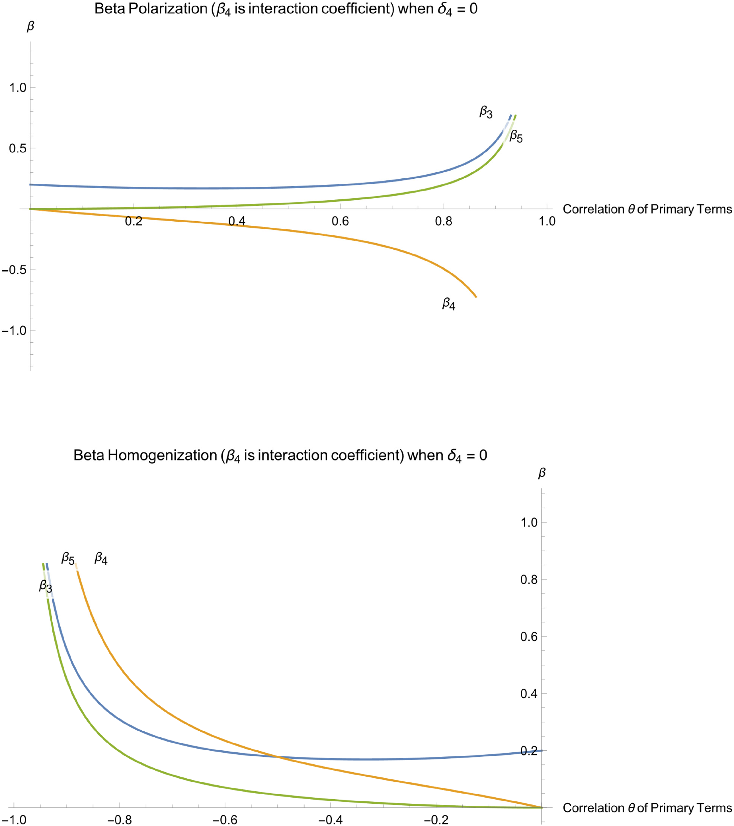
(a and b) Expected Values of Estimated Beta Coefficients from Equations 24, 25 and 28.

Because Equation 28 is linear and additive in terms of δ₃ and δ₅, as per Conclusion 2, the curve for the estimated β₄ in Figure 1a remains identical for any δ₃ + δ₅ = 0.2. Further, the β₄ curve retains the same shape for any value of δ₃ + δ₅ > 0. The only difference will be that the y-axis will require rescaling. Figure 1a generalizes to δ₃ + δ₅ < 0 with the only additional difference that the three curves are reflected against the x-axis: β₄ will move upwards towards positive infinity as θ increases while β₃ and β₅ will move downwards. Beta polarization remains.

Figure 1b shows beta homogenization for the opposing factor form of the Common Factor DGP with δ₃ = 0.2 still being the only true effect. Beta homogenization is now evident from the figure, with the estimated β₃ and β₅ swinging up towards positive infinity in a perfect mirror image of Figure 1a, but β₄ also moves towards positive infinity. All the values for β₃ and β₅ will be the same for correlation −θ as for θ. β₄ will have the same absolute magnitude for −θ as for θ, but the opposite sign, and the same likelihoods of being type 1 interaction errors. All generalizations from the previous paragraph hold for Figure 1b, due to linearity and additivity.

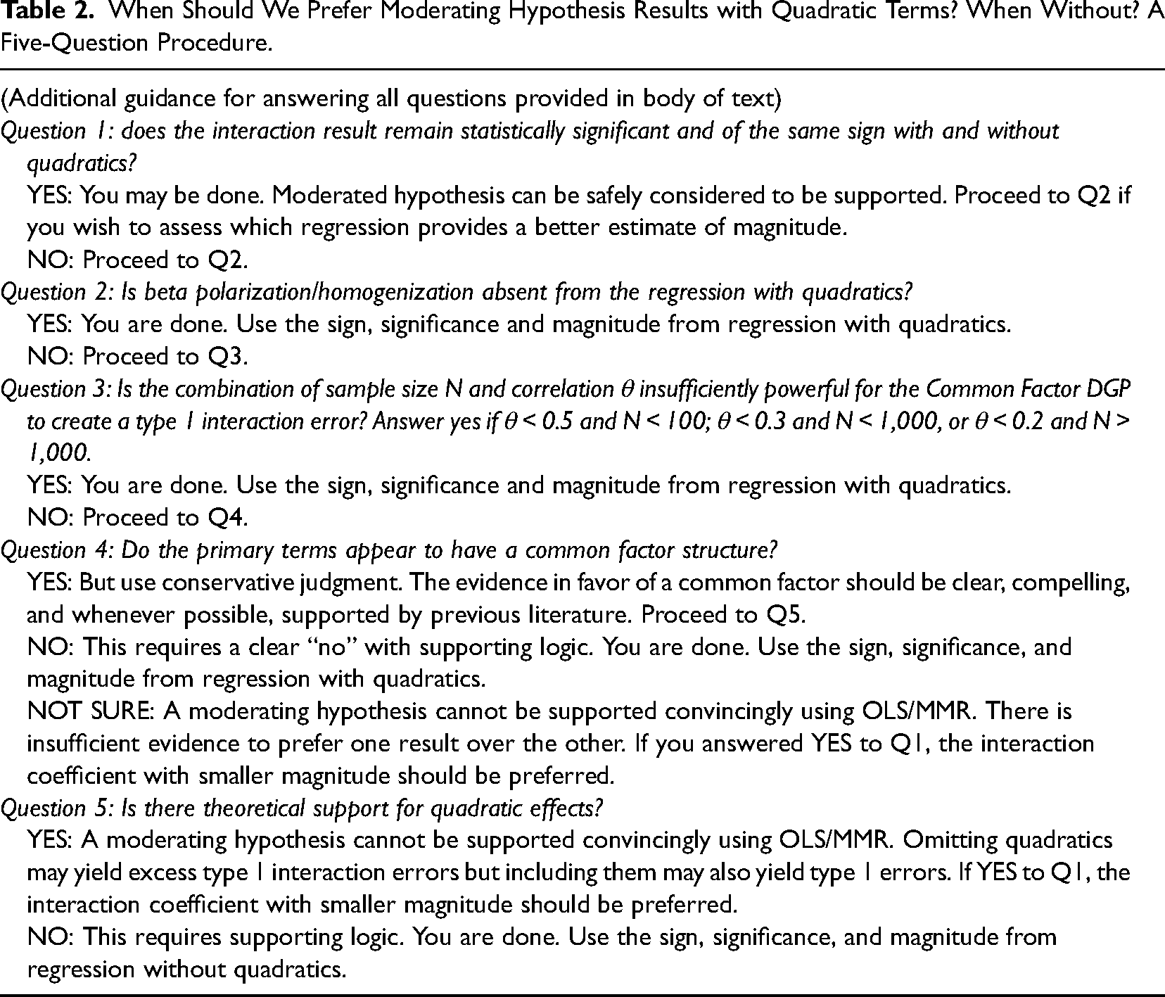
Five Questions that Determine Whether to Include Quadratics

Below we provide a five-question procedure that researchers should follow to determine whether to prefer moderated regressions with or without quadratics. Researchers should present, in full, and in separate columns, regression results both with and without quadratics regardless of which set of results is finally the preferred one. The cost in terms of analysis and print space is minimal, while the benefit in terms of avoiding type 1 errors is substantial. We discourage the unfortunately widespread practice where researchers present an interaction result from a regression without quadratics in the same column as quadratic coefficients from a different regression. Finally, we encourage researchers to include all interactions and quadratic terms in the correlation table.

Question 1: Does the Interaction Result Remain Statistically Significant and of the Same Sign with and without Quadratics?

If yes, we can safely consider an interaction hypothesis to be supported. If the researcher's sole goal is to support a hypothesis, no further analysis is necessary. If the coefficient magnitudes differ substantially and researchers wish to know the more likely true magnitude, they should answer the four questions below. But, if the answer to Q1 is “no,” the four questions require answers, even for a simple hypothesis test.

Question 2: Is Beta Polarization/Homogenization Absent in the Regressions with Quadratic Terms?

If the correlation of the primary terms is positive, is the interaction term coefficient's sign in the same direction as those of the quadratic terms from the same regression? If the correlation of the primary terms is negative, is the interaction term coefficient's sign opposite those of the quadratic terms from the same regression? If either of these statements is true, we can dismiss the possibility of a Common Factor DGP type 1 interaction error. Interaction coefficients with the quadratics included should then be the preferred results used for the possible support of a hypothesis, with no further analysis necessary. If neither statement is true, then we will need to answer the additional three questions to identify the preferred regression results.

Question 3: Is the Combination of Sample Size N and Correlation θ Insufficiently Powerful for the Common Factor DGP to Create a Type 1 Interaction Error?

We make recommendations based on our analysis of the Common Factor DGP, Equation 48, and small to medium effects sizes from Cohen (1988). First, absolute values of correlations |θ| < 0.5 appear too small to generate type 1 errors at a 20% rate when N < 100. Second, if N > 100, only correlations |θ| < 0.3 are too small to generate type 1 errors for N < 1,000. Finally, only correlations |θ| < 0.2 are too small to generate type 1 errors for N < 1,000.

Question 4: Do the Primary Terms Appear to Have a Common Factor Structure?

We discussed three identifiable forms of a common factor in the section titled “Qualitative Assessment of the Presence of a Common Factor.” A common factor a likely possibility in a set of data if: (1) the primary term variables are conceptually or structurally related to a common antecedent, which includes the possibility that one primary term variable is, in part, a function of the second variable, (2) proxy variables or a common method are used, because these may have common correlations with omitted variables and with a source of error, or (3) primary terms are multi-item scales and individual items are similar across the scales, particularly if the scales have not met the requirements of discriminant validity.

We also discussed the identification of an idiosyncratic component with a separate quadratic effect on the DV. In practice, the idiosyncratic term may be any omitted variable with quadratic effects on the DV, correlated with one primary term more than the other, with effects independent of the common factor.

Question 5: Is there Theoretical Support for Quadratic Effects of the Primary Terms?

While previous work has emphasized including non-linear functional forms of variables only if supported by theory (e.g., Aiken & West, 1991; Balli & Sørensen, 2013; MacCallum & Mar, 1995; Su et al., 2019), our analysis points to an insurmountable conundrum if the answer to Q5 is “yes.” There is simply no credible means, as of this writing, to establish a preference between the contradictory results for the interaction coefficient if Q1–Q4 were otherwise unable to resolve the matter. On the one hand, omitting quadratics may yield excess type 1 interaction errors as per Cortina (1993) when theory suggests the quadratics will have true effects. On the other hand, including quadratics may also yield type 1 interaction errors, even if their effects are very real and theoretically motivated, due to the possibility of a dependent variable generated by the Common Factor DGP.

If the answer is “no,” that is, primary term effects are likely to be approximately linear, researchers should prefer interaction results that omit quadratic effects. If researchers wish reviewers and readers to accept their judgment regarding supported interaction hypotheses, it is their responsibility to provide logic convincing to reviewers. What reviewers are convinced by will of course vary and it is beyond the scope of this paper to provide specifics in that regard. Nonetheless, the issue requires a clear and explicit discussion in published research so that readers can incorporate the logic in replications and extensions of the original work.

The Six Example Papers Revisited

In Table 1, we summarized six papers that presented two full sets of moderated regression results, with and without quadratic terms, a practice we would like to see in more empirical work. We revisit the six papers now in light of the conclusions that we have codified into Table 2 to aid empirical researchers to make appropriate decisions whether to prefer moderated regression results with or without quadratic terms.

Table 2.

When Should We Prefer Moderating Hypothesis Results with Quadratic Terms? When Without? A Five-Question Procedure.

(Additional guidance for answering all questions provided in body of text)

Question 1: does the interaction result remain statistically significant and of the same sign with and without quadratics?

YES: You may be done. Moderated hypothesis can be safely considered to be supported. Proceed to Q2 if you wish to assess which regression provides a better estimate of magnitude.

NO: Proceed to Q2.

Question 2: Is beta polarization/homogenization absent from the regression with quadratics?

YES: You are done. Use the sign, significance and magnitude from regression with quadratics.

NO: Proceed to Q3.

Question 3: Is the combination of sample size N and correlation θ insufficiently powerful for the Common Factor DGP to create a type 1 interaction error? Answer yes if θ < 0.5 and N < 100; θ < 0.3 and N < 1,000, or θ < 0.2 and N > 1,000.

YES: You are done. Use the sign, significance and magnitude from regression with quadratics.

NO: Proceed to Q4.

Question 4: Do the primary terms appear to have a common factor structure?

YES: But use conservative judgment. The evidence in favor of a common factor should be clear, compelling, and whenever possible, supported by previous literature. Proceed to Q5.

NO: This requires a clear “no” with supporting logic. You are done. Use the sign, significance, and magnitude from regression with quadratics.

NOT SURE: A moderating hypothesis cannot be supported convincingly using OLS/MMR. There is insufficient evidence to prefer one result over the other. If you answered YES to Q1, the interaction coefficient with smaller magnitude should be preferred.

Question 5: Is there theoretical support for quadratic effects?

YES: A moderating hypothesis cannot be supported convincingly using OLS/MMR. Omitting quadratics may yield excess type 1 interaction errors but including them may also yield type 1 errors. If YES to Q1, the interaction coefficient with smaller magnitude should be preferred.

NO: This requires supporting logic. You are done. Use the sign, significance, and magnitude from regression without quadratics.

First, we cannot support Ganzach’s (1997) hypothesis of a negative interaction coefficient. The answer to Question 1 in Table 2 is “no” because the interaction coefficient's sign flipped from positive to negative when he added quadratic terms. The answers to Questions 2 and 3 are also “no.” Beta polarization is present, and the primary term correlation θ = 0.67. Further, as shown in Table 1, and supported by Schwartz and Mare (2005), there is likely a common factor at play related to parents’ desire for educational achievement. The idiosyncratic component might be present if a parent of one gender typically had a quadratic effect on its own that would be independent of the common factor. The fulfillment of these criteria would allow a “yes” answer for Q4. Finally, the fact that both primary term variables are counts of years of education, and the dependent variable is an expectation of years of education, there little reason to believe, theoretically a priori, in a curvilinear effect. The effect could be close to linear. Therefore, as per Q5, we should prefer the result without quadratics. Ganzach (1997) had no hypothesis for a positive moderation effect so we should make no inference beyond the fact that his hypothesis of a negative effect is unsupported.

Second, we conclude that Ganzach et al.’s (2000) negative and statistically significant interaction term finding is valid because, as per the first question of Table 2, it holds whether quadratics are included or excluded. There may be a common factor because educational motivation is in part a function of cognitive ability, but the robustness of the result outweighs the possibilities of false interaction positives due to omitting quadratics (Canonical DGP) or including them (Common Factor DGP). We note that Ganzach et al. (2000) argue in favor of a logit model in the study, but we limit the analysis to their OLS/MMR results.

Third, we conclude that Ganzach et al.’s (2013) positive and statistically significant interaction effect is valid because it does not change when they added quadratics, as per Q1. The interesting question here is the magnitude of the effect—it grows fivefold when they added the quadratic terms—and so we proceed to subsequent questions. The answers to Questions 2 and 3 are “no.” Beta polarization is present, and the primary term correlation θ = 0.5. Further, as stated in Table 1, and supported by Schmidt and Hunter (2004), there is a common factor at play, because occupational complexity is in part a function of mental ability. If omitted variables exist that might explain a part of the DV and might partially explain occupational complexity, but not mental ability, then the Common Factor DGP is present. This would allow a “yes” answer for Q4. Finally, Ganzach et al. (2013) provide clear theory for a concave relationship between ability and wages, but they provide none for a non-linear relationship between occupational complexity and wages. Therefore, as per Q5, we should prefer the result without quadratics and its smaller magnitude.

Fourth, due to a “no” answer to Q1, we agree with Cole et al. (2011) that the negative interaction result should not be considered valid without further investigation. But we do not agree that the model with quadratics is necessarily an improvement. Regarding Q2, beta homogenization with a negative correlation is present. As for Q3, θ = −0.70 is sufficiently high, regardless of sample size N, to be concerned about the effects of common factors. We continue on to Q4. Cole et al. (2011) have clearly identified structural commonalities of level and dispersion that may play a role similar to a substantive common factor. But because these are not a common factor per se, a separate analysis is required that is outside our scope.

Fifth, we agree with Cero et al.’s (2015) conclusion from their first sample that the positive and marginally significant interaction effect cannot be accepted without also considering quadratics. But, because the answer to Q1 is “no,” we cannot agree that the model with quadratics is necessarily the superior one. The answers to Questions 2 and 3 are “no.” Beta polarization is present, and the primary term correlation θ = 0.57 implies we must consider the possibility of a Common Factor DGP. Further, as stated in Table 1, there is a common factor because the two measures have related items in common (e.g., Van Orden et al., 2012); there is a lack of discriminant validity. If there are also substantive idiosyncratic terms among the individual items of one scale, then a “yes” answer is possible for Q4. The lack of theory for the quadratics as per Q5 allows us to conclude that results without quadratics are preferable in terms of magnitude. In their second sample there is no statistical significance with or without quadratics and there is no need to analyze further.

Sixth, and finally, Ping’s (1996) motivation for his study is that previous mixed results with his dependent variable might be the result of omitted quadratic effects. Yet in his study the interaction term appears significant without quadratics as well as with them. The magnitudes are similar, and the signs are the same, thus we should accept Ping's hypothesis based on Q1.

Limitations, Extensions and Conclusions

Limitations and Extensions

By assuming standard normal primary terms, we ensured that they are mean-centered; this fact causes no loss of generality for the results (Aiken & West, 1991; Edwards, 2009; our Conclusion 1). We have demonstrated that substantial excess type 1 interaction errors may occur even for the ideal case of mean-centered, standardized, normally distributed variables.

The conclusions of this paper extend to interaction terms of more than two linear primary terms. In the case of three-way interactions, for example, we found via simulations, not shown, that we must worry not only about cubic effects of individual primary terms masquerading as three-way interaction term effects, but also about true effects of compound interaction terms of quadratic and linear primary terms influencing effects of the three-way term.

Beyond the quadratic effects that we considered, square root and logarithmic effects of the primary terms may also falsely affect interaction term coefficients. These non-linear forms do not lend themselves to linear algebraic analysis in a straightforward manner. Simulations of these functional forms, not shown, suggest that they are less problematic than omitted or included quadratic terms. Even sample sizes of 2,000 were not capable of generating consistent type 1 errors of interaction terms for square-root effects of either DGP. For logarithmic effects, the incidence of type 1 errors was less frequent than for the case of quadratic effects.

Further, while we restricted our analysis to second-order polynomials with continuous primary terms, the type 1 error problem can be worse for dichotomous variables (e.g., “Artificial Dichotomization of Continuous Moderators;” Aguinis et al., 2017). Dichotomous variables that proxy for latent continuous variables, for example high school graduation for education, are problematic because the researcher has no ability to create a quadratic term to control for a curvilinear latent effect. Any curvilinear effect of the underlying continuous primary term will necessarily be transferred to an interaction term, if present.

Finally, we cannot analyze maximum likelihood-based methods such as logit, probit, Poisson, and hazard models using linear algebra and Cramer's Rule. Simulations indicate that the same issues we showed for OLS/MMR are also of concern in these alternative models. Formally extending the results of this paper to maximum-likelihood methods and establishing the exact nature of any additional complications would represent a productive avenue for future research.

Three Applications for Future Work

Three OLS/MMR applications in organizational methods research might benefit from our analysis. First, Lai et al. (2013) analyze whether common method variance (CMV) creates type 1 errors in hierarchical linear modeling in the form of cross-level interaction effect false positives. Those authors conclude from simulations that, on the one hand, if a true cross-level interaction exists, CMV will tend to create a type 2 rather than a type 1 error. On the other hand, if there is no true interaction, they argue that CMV will not create a false effect. But they have not considered quadratic effects at the group level, which may play the role of the idiosyncratic term. Further, the model they estimate (Equation 2) exhibits a second-degree polynomial structure and we can thus view CMV as a common factor. Their model might be amenable to linear algebraic analysis such as that presented here.

Second, Edwards (2001) and Edwards and Parry (1993) have posited that polynomial regressions and response surface modeling are superior alternatives to analyses of difference scores when examining congruence effects. Instead of a single difference variable, the dependent variable can be regressed on the five variables of the second-order polynomial: the primary terms, their quadratics, and an interaction term. After conducting such a regression, Edwards and Parry (1993) argue that researchers should examine the slope and curvature along the congruence and incongruence lines to test hypotheses. According to those authors, the estimated β₁ − β₂ and β₃ + β₄ + β₅ represent the slope and the curvature of the surface along the congruence line where x₁ = x₂. The coefficients β₁ − β₂ and β₃ − β₄ + β₅, respectively, represent the slope and the curvature of the surface along the incongruence line (x₁ = –x₂). A convex curvature is consistent with a meaningful increase in a dependent variable when x₁ and x₂ are congruent and is evidenced by a negative and statistically significant curvature (β₃ − β₄ + β₅ < 0) along the incongruence line, and non-significant slope (β₁ + β₂) and curvature (β₃ + β₄ + β₅) along the congruence line.

However, Conclusion 3 states that, in the case of a Common Factor DGP, beta polarization will artificially push the coefficient of β₄ in the opposite direction from the quadratic coefficients β₃ and β₅. This reality suggests that the response surface method may yield false conclusions in favor of convex curvature, for example, if β₃ and β₅ are pushed in a negative direction and β₄ is pushed in a positive direction. We recommend further analysis.

Third, there is a similarity between moderated mediation models and the analysis here because mediation necessarily implies correlation among primary terms. If data are generated perfectly as per the standard partial mediation model, then the Canonical and partial mediation DGPs are equivalent. Strict causality and a lack of omitted variables in the mediator equation are key to this equivalence. In this case there will be no beta polarization. Aguinis et al. (2017) discuss the importance of strict causality in the mediator equation, and we provide another reason: if there is reverse causality or an omitted variable in the mediator equation, the underlying DGP becomes similar to the Common Factor DGP and may cause beta polarization.

Summary and Implications

We have conducted a detailed and original linear algebraic analysis of two data generating processes to provide a new perspective on the question of whether researchers should prefer results that include or exclude quadratics when testing hypotheses of moderation. It has been well-known that real but omitted quadratic effects of correlated primary variables may create type 1 errors in the form of false interaction effects. The analytical contribution here is the demonstration that the existing “state of the art” solution of always including quadratic terms may create the exact problem it attempts to solve: if a Common Factor DGP has generated the DV, including quadratic terms may create excess type 1 interaction errors rather than eliminate them.

We applied our analysis to create a five-question procedure, summarized in Table 2, to help scholars studying interaction effects decide when to prefer results with, and when without, quadratic terms. Research should always begin with full presentation of separate regression results both with and without quadratic terms. Reviewers should insist on viewing both sets of results. From there researchers should follow Table 2 to build the strongest case for the preferred regression specification. Following these procedures will allow a field of research to address conflicting findings early on in the scientific process, well before journals publish non-robust findings that may be type 1 interaction errors and well before the field enshrines them as “knowledge.” At that late point, multiple non-replications might be required to cast doubt on their veracity.

The conclusions of our analysis highlight the need for organizational scholars to consider in greater depth the implications of the typical OLS assumption that the Canonical DGP has generated the dependent variable. Organizational and social science research accepts the fact that often we cannot accurately observe all variables that influence a dependent variable, despite its inconsistency with the Gauss-Markov assumptions and with the Canonical DGP. This inconsistency is often benign; however, in the case of interaction terms, the possibility of false interaction positives represents a critical concern. Type 1 errors may become commonplace in realistic settings. More generally, OLS regression can be far messier than we often believe. We should be more skeptical of basic findings in OLS-based research and subject these results to more scrutiny when common factors are present among independent variables.