Sage Journals: Discover world-class research

Abstract

Inflection points, kinks, and jumps identify places where the relationship between dependent and independent variables switches in some important way. Although these switch points are often mentioned in management research, their presence in the data is either ignored, or postulated ad hoc by testing arbitrarily specified functional forms (e.g., U or inverted U-shaped relationships). This is problematic if we want accurate tests for our theories. To address this issue, we provide an integrative framework for the identification of nonlinearities. Our approach constitutes a precursor step that researchers will want to conduct before deciding which estimation model may be most appropriate. We also provide instructions on how our approach can be implemented, and a replicable illustration of the procedure. Our illustrative example shows how the identification of endogenous switch points may lead to significantly different conclusions compared to those obtained when switch points are ignored or their existence is conjectured arbitrarily. This supports our claim that capturing empirically the presence of nonlinearity is important and should be included in our empirical investigations.

Keywords

inflection points kinks statistical jumps threshold estimation nonlinearity Hansen’s method

An important empirical challenge faced by management scholars consists in the choice of model specification. This choice can have dramatic effects for the sign and magnitude of estimated relationships and, therefore, for the accuracy of our analyses and their implications. In practice, most empirical studies in management assume (implicitly or explicitly) a linear relationship between dependent and independent variables. Examples include the effects of strategic and market complementarity on the performance of acquisitions (Finkelstein, 2009), the impact of female managerial representation on a firm's innovation (Foss et al., 2021) or market performance (Dezsö & Ross, 2012), the relationship between generosity and status attainment (Ouyang et al., 2018), and the effect of ownership concentration on IPO performance (Bruton et al., 2010). Linear model specifications are attractive because they ease the interpretation of results and the testability of hypotheses.

Linearity, however, may hold up only over a subset of values. For example, the behavioral theory literature finds that, when underperforming, firms tend to search for solutions based on newly acquired, and therefore riskier, knowledge (Greve, 2003; Shinkle, 2012). However, when performance drops far below aspirations, firms are shown to shift away from innovative solutions and to redirect their attention to risk-averse solutions (Miller & Chen, 2004; Shimizu, 2007; Staw et al., 1981). This is just one example illustrating the presence of a “switch” point delimiting the range of values where a specific type of relationship between the dependent variable (Y) and an independent variable of interest (X) holds. Researchers who ignore the presence of the above switch point will estimate one coefficient (for X) when they should be estimating separate coefficients before and after the switch point. In other words, the coefficient they will estimate will be upward or downward biased, and akin to a weighted average of the non-estimated separate coefficients, but with unknown weights and no real meaning.

Ubiquitous in our data, switch points are points that distinguish ranges of values where the relationship between dependent and independent variables predicted by the model changes in some important way. Switch points may take a variety of forms, and may manifest in the investigated relationship as inflection points, kinks, or jumps. The same relationship between the dependent variable and an independent variable of interest may exhibit one such switch point or multiple of them, and they may be similar or of different types. In general, the presence of switch points in empirical management research is either ignored or postulated ad hoc. In fact, across a broad spectrum of management areas, researchers like Bowen (2012), Grant and Schwartz (2011), Huselid and Day (1991), Le et al. (2011), Pierce and Aguinis (2013), have emphasized the problematic implications of neglecting nonlinearities in the data or making arbitrary assumptions about them, as doing so may substantially influence the results of our analyses and lead to potentially wrong conclusions.

The purpose of this article is threefold. First, we emphasize why a test for a possible nonlinear relationship between dependent and independent variables is necessary for the accurate choice of model specification. Second, we provide a three-steps approach that allows for conducting such a test in a simple but accurate way. Third, we contrast our approach to alternative possible methods to show and compare the advantages and disadvantages of each. Our goal is to provide an integrative framework to help researchers with detecting possible non-linearities in the data and selecting accordingly the most suitable estimation method. For example, a researcher may try to test for a hypothesized nonlinearity by adding a squared term to the model. This, however, implies that the researcher assumes the existence of a continuous curvature. Yet, the true shape of the relationship between dependent and independent variables may exhibit a discontinuous jump and, therefore, her assumption would yield inaccurate results. Our approach, instead, allows for the discovery of a possible switch point without the researcher having to guess whether such a nonlinearity exists, its location, and its type.

In the spirit of Ostroff (1993), Dul (2016), and Rönkkö et al. (2021), our contribution fits with research dealing with unknown potential limitations of data and existing statistical tools. Our approach overcomes a number of challenges associated with the use and interpretation of linear models and sample splitting, and it allows for comparing our theories with what the data actually say, without our theoretical beliefs influencing the results spuriously.

Switch Points in Management Research

Switch points identify situations where the relationship between two variables (typically, the dependent variable and an independent variable of interest) changes in some important way. Tong (1978) defined switch points as “statistical thresholds,” a terminology routinely used in mathematics, statistics, and economics. Yet, in management the word “threshold” is often associated to a different meaning. Thus, we adopt the term “switch points” to avoid possible confusion. Switch points include inflection points, kinks, and jumps. Table 1 shows illustrative plots for each type of switch point, as well as some illustrative examples where more than one switch point can be seen.

Table 1.
Types of Switch Points.

Graphical illustrations Definition Implications

Panel A: Inflection points

An inflection point is a switch point on a continuous function where a change in the direction of the curvature occurs Statistical significance exists before and/or after the switch point

Panel B: Kinks

A kink is a switch point on a continuous function where both sides are straight lines Statistical significance may exist only before or after the kink (top plots) or before and after the kink (bottom plots)

Panel C: Jumps

A jump is a switch point that identifies a discontinuity in a function Statistical significance may or may not exist before and/or after the jump

Panel D: Multiple switch points

Functions may exhibit combinations of two or more switch points, of similar or different types Statistical significance may exist before and/or after each switch point, depending on the type of each switch point

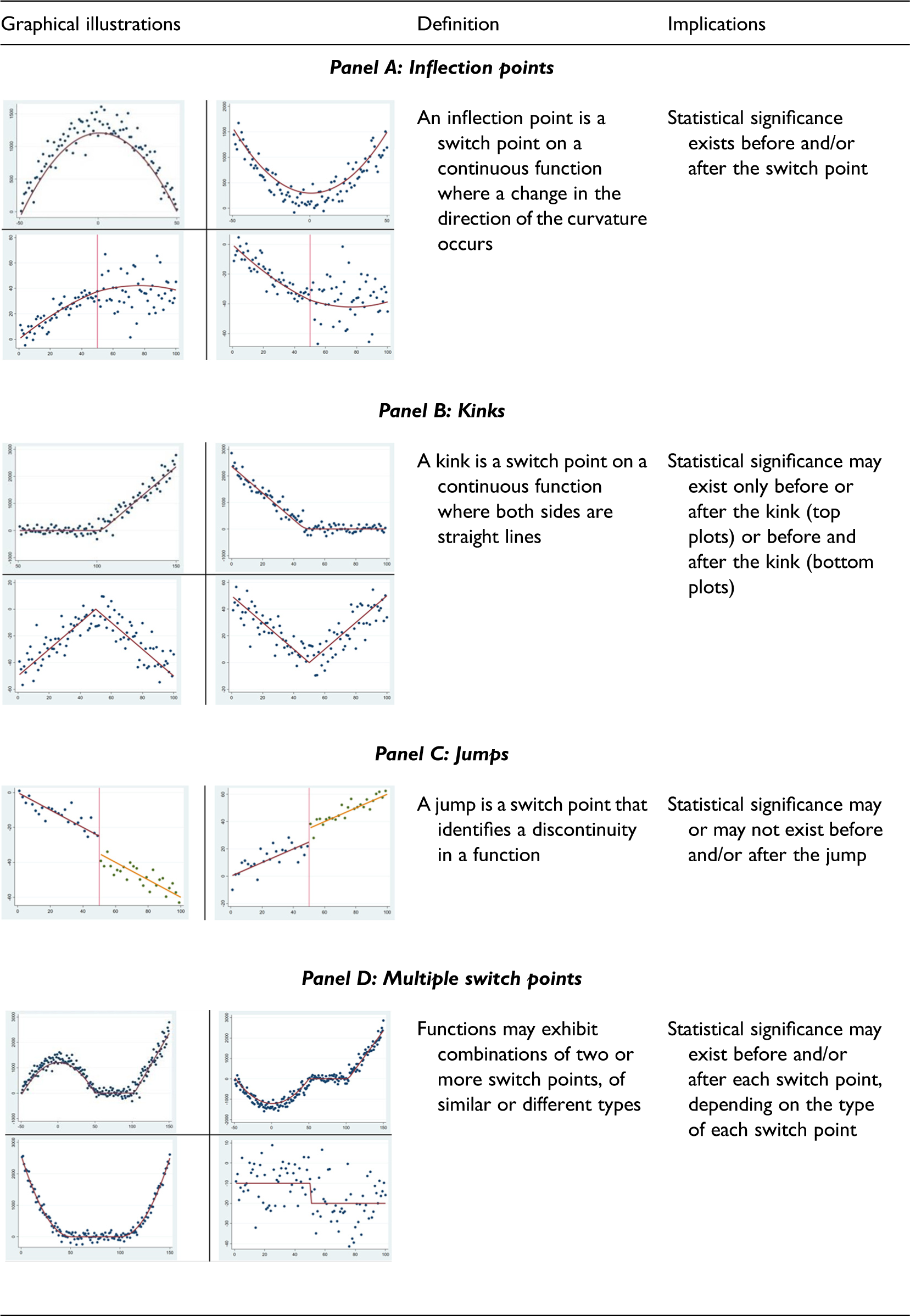
The first group of switch points shown in Table 1 Panel A consists of inflection points. Among possible types of switch points, inflection points are the most commonly referred to in management theory and tested for empirically (e.g., Grant & Schwartz, 2011; Pierce & Aguinis, 2013; Rapp et al., 2014; Yu et al., 2019; Zahavi & Lavie, 2013, among many others). Inflection points are related to concavity, and may identify a significant change in the curvature of a U (or inverted U or S) shaped relationship. In principle, they can be captured by adding polynomial terms to a regression, not necessarily squared terms only. This means, however, that inflection points are relevant only when a continuous curve is present.¹ Thus, they represent only a subset, albeit a large one, of all the potential situations in which the relationship between two variables changes.

Switch points, however, also include cases in which a kink or a jump emerge in a relationship between two variables, regardless of significance levels before and after the identified switch point. These types of switch point cannot be captured by looking for inflection points. Table 1 Panel B illustrates kinks, situations where the relationship between two variables goes (i) from zero slope to positive or negative slope, but both sides are straight lines; or (ii) from having a positive (negative) slope to having a negative (positive) slope, but both sides are straight lines. In the first case, the relationship between the two variables is insignificant over the horizontal line before the switch point, but becomes significant when the straight line begins going up or down. In the second case, the relationship between the two variables is significant before and after the switch point, but with different coefficients and possibly different signs. In all cases, however, there is no curvature. Thus, adding polynomial terms to a regression will not capture kinks.

Table 1 Panel C illustrates jumps. A jump identifies a discontinuity in the relationship between two variables. Similar to a kink, when a jump is present, the relationship between two variables may be (i) insignificant before (after) the discontinuity but significant after (before) the discontinuity, or (ii) significant on both sides of the discontinuity. The sign of the estimated coefficients of the independent variable before and after the discontinuity may change or remain the same. Importantly, as in the case of kinks, in all cases of jumps, there is no curvature, and thus adding polynomial terms will not capture the switch point.

Finally, Table 1 Panel D provides some examples where multiple switch points are present. These switch points can be all of the same type, or belong to different types, and we can imagine an infinite number of combinations where multiple inflection points, or multiple kinks or jumps, or a combination of kinks, jumps and inflection points exist. In those cases, the sign and statistical significance of the relationship between two variables will change over the range of data considered, and will depend on the nature of the switch points present. In sum, switch points encompass a large set of “change” points which address a variety of cases with sudden and multiple changes in slope, where the empirical relationship between two variables changes magnitude, direction and/or significance.

Since switch points represent a substantially broader category than inflection points, the problems and potential for error are actually larger than standard practices in the field would let us imagine. In addition to the challenges associated with the existence of different types of switch points, the latter may be problematic because their existence and position are often unknown. In fact, when switch points are included in the analysis, they are typically associated with sample splits based on an apparently known switch point in the relationship between variables. For example, an investigation of performance differences between U.S. small and medium enterprises (SMEs) and large firms is an example of a known switch point based on some commonly accepted criteria for dividing firms into large or small. Unfortunately, however, switch points are often not known a priori, and present in relationships between variables that do not lend themselves to unambiguous subgroupings. In the ubiquitous case of unknown switch points, researchers typically select where to split the sample in an arbitrary way, either by following previous literature (e.g., Flammer, 2015), or by looking at descriptive statistics or graphical displays of sampled data (e.g., Kogut et al., 2014). Even if theoretically or empirically grounded, these practices may still fail to properly identify the real value at which a switch point is located in the data and, as a result, lead to inaccurate conclusions.

When their presence is suspected but not known a priori, an accurate identification of switch points requires their proper empirical estimation. Unknown switch points, however, are unidentifiable with standard statistical tests (Hansen, 1992, 1996).² We emphasize the need to search for the existence of endogenously determined switch points in the data and provide a simple and accurate three-steps approach to address the problem of unknown switch points in management research.

Dealing with Switch Points in Management Research

The idea behind modeling switch points is simple. We start with a basic linear model specification:
$y = X^{'} β + Z^{'} δ + ε;$
(1)
where y is a continuous dependent variable (possibly bounded within a certain range of values), X is the vector of control variables, β is the vector of coefficients associated to control variables, Z is the independent variable (i.e., the regressor of interest), δ is the coefficient associated to the independent variable, and ε is an error term that follows a Normal distribution with zero mean and variance equal to σ².

In the presence of a switch point known a priori, Equation (1) becomes:
$y = X^{'} β + Z^{'} δ_{1} + ε, i f t \leq γ .$
(1a)
$y = X^{'} β + Z^{'} δ_{2} + ε, i f t \leq γ .$
(1b)
where δ₁ and δ₂ are the coefficients of the independent variable Z before and after the switch point γ, respectively, and t is the continuous variable whose distribution displays the switch point γ.³

Thus, to test for the presence of the switch point, it is possible to conduct a standard Wald test on the null hypothesis H₀ that the coefficients δ₁ and δ₂ are not statistically different (i.e., H₀: δ₁ = δ₂). Under H₀, the models (1a) and (1b) “collapse” into the model in Equation (1) which can be estimated by means of Ordinary Least Squares (OLS).

If the switch point is not known a priori, however, the above standard Wald test cannot be conducted (Davies, 1977, 1987; Hansen, 1996) because the switch point γ is unknown. In this situation, the potential existence of switch points goes untested (Andrews & Ploberger, 1994).

When dealing with switch points, management researchers use different approaches including mathematical models (e.g., Chatain, 2011), simulation-based analyses (e.g., Lieberman et al., 2017), and experimental settings (e.g., Agarwal et al., 2010). Switch points have been even used to build datasets (e.g., Reitzig & Wagner, 2010), and to test hypotheses (Hahn et al., 2001). Yet, formal empirical assessments of their presence are extremely rare. In fact, a full-text search on multiple terms related to switch points in top management journals confirmed that, although terms such as inflection points and nonlinearity are ubiquitous across journals, attempts to estimate them using approaches that do not require a priori assumptions about the shape of a relationship between variables are lacking.⁴

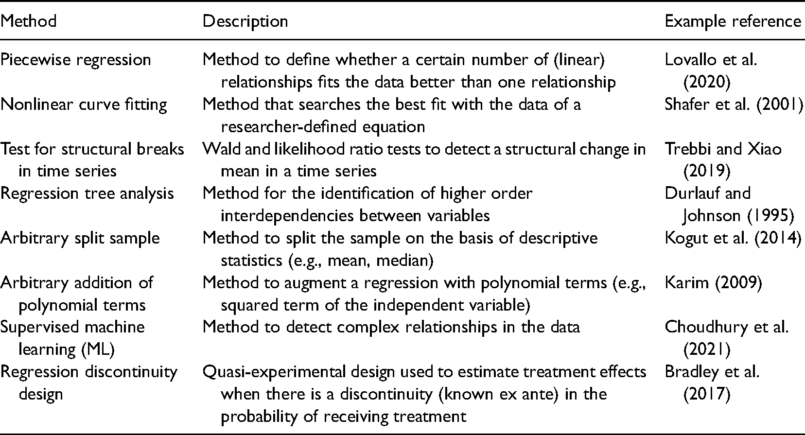
Indeed, most scholars who test for nonlinearity do so by imposing a priori constraints on the model specification. For instance, in piecewise regressions the optimal number of relationships fitting the data is decided a priori (two in the vast majority of cases). Similarly, nonlinear curve fitting assumes a researcher-defined equation to represent the model that best fits the data. In an alternative, Choudhury et al. (2021) argue that supervised machine learning (ML) methods can help researchers to formulate better hypotheses grounded in data, which could then be tested deductively using traditional econometric techniques. However, in their pure application, ML methods pick the functional form that best predicts the dependent variable (y), given the independent variable of interest (Z) and the control variables (X). Thus, they are data-driven in the sense that the proposed model is inferred entirely from the data.

Other methods are able to identify only one type of switch point. For example, regression discontinuity design (RDD) (Hahn et al., 2001) estimates whether there is a statistically significant jump in the effect of an independent variable (called “treatment”) on the dependent variable. This jump, however, must be in the surroundings of a known discontinuity in the probability of the dependent variable being subject to the treatment. For example, Bradley et al. (2017) used RDD to investigate the relationship between unionization and firm innovativeness by using cases where a union election passed or failed by a small margin of votes. Since the context of firms where election outcomes are close can be assumed to be similar, election outcomes provide a known discontinuity in the data. RDD leverages that discontinuity to assess the effect of unionization on innovativeness post-elections. Table 2 provides a list of methods commonly used in the management literature to account for nonlinearity in the data, as well as a brief description and a reference to an empirical application.

Table 2.
Main Methods Used to Detect Switch Points.

Method Description Example reference

Piecewise regression Method to define whether a certain number of (linear) relationships fits the data better than one relationship Lovallo et al. (2020)

Nonlinear curve fitting Method that searches the best fit with the data of a researcher-defined equation Shafer et al. (2001)

Test for structural breaks in time series Wald and likelihood ratio tests to detect a structural change in mean in a time series Trebbi and Xiao (2019)

Regression tree analysis Method for the identification of higher order interdependencies between variables Durlauf and Johnson (1995)

Arbitrary split sample Method to split the sample on the basis of descriptive statistics (e.g., mean, median) Kogut et al. (2014)

Arbitrary addition of polynomial terms Method to augment a regression with polynomial terms (e.g., squared term of the independent variable) Karim (2009)

Supervised machine learning (ML) Method to detect complex relationships in the data Choudhury et al. (2021)

Regression discontinuity design Quasi-experimental design used to estimate treatment effects when there is a discontinuity (known ex ante) in the probability of receiving treatment Bradley et al. (2017)

A notable departure from the methods listed in Table 2 comes from Heeley and Jacobson (2008). These authors investigate whether the reaction of financial markets to corporate inventions depends on the recency of knowledge inputs used for those inventions. Specifically, Heeley and Jacobson (2008) augment a baseline financial valuation model with a dummy variable capturing whether the median age of knowledge inputs is located before or after a certain switch point, as described in our equations (1a) and (1b). Heeley and Jacobson recognize that, since the number of switch points and their values are not known a priori, their empirical determination cannot be conducted by means of standard statistical tests.⁵ To address this issue, they follow Hansen’s (1999) estimation method and use a likelihood ratio (LR) test to detect critical unknown switch points.⁶ The contribution by Heeley and Jacobson (2008) is important because, to our knowledge, this is the only article to date that leverages Hansen's method. A more recent version of that method (Hansen, 2000) is used as part of the approach we propose in this article.

A Suggested Approach for Identifying and Handling Switch Points

The approach we propose is a three-step procedure that allows researchers to overcome a number of challenges associated with the use and interpretation of linear models and sample splitting. Specifically, our approach is based on the idea that theory should drive empirical strategies but, at the same time, empirical evidence should challenge our theoretical arguments. In a nutshell, step 1 is necessary to preliminarily check the data for the presence of possible outliers or errors.⁷ Step 2, consists in the application of Hansen’s (2000) method to accurately test for the presence of one or possibly more unknown switch points, and identify their values endogenously from the data. Finally, step 3 is necessary to identify jumps or discontinuities in the surroundings of the switch points potentially identified in step 2.

Overall, our approach constitutes a precursor framework that researchers will want to conduct before deciding which model specification and estimation method may be most appropriate. The combination of graphical analyses and formal tests included in our approach allows researchers to establish the presence, location, and type of switch point. Then, together with theory, our approach informs whether splitting the sample is necessary and, if so, where the split should happen (i.e., at which value of the variable whose distribution displays the switch point), what estimation methods are more appropriate, and how to test for parameter significance and calculate the associated test statistics and confidence intervals. We now discuss each step of the approach in details, and provide all necessary Stata commands to execute it.

Step One

The first step of our approach consists of a graphical inspection of the data to visualize possible nonlinearities, and the range of values at which a switch point seems to be present. We suggest the use of smoothing methods, such as a locally weighted regression (as also highlighted by Heeley & Jacobson, 2008) or a Kernel-weighted local polynomial regression.⁸ Unlike standard linear regressions, smoothing methods do not specify an a priori functional form to proxy the relationship between dependent and independent variables. Instead, they are agnostic in the sense that they allow the data points to give an indication of the form of the above relationship.

Step 1 is especially important when no priors about the shape of the relationship between the dependent and an independent variable exist, or when previous literature is inconclusive about the investigated relationship. Still, even when established theories exist, step 1 is very important as it also allows for a preliminary comparison between a theory's expected prediction and the data. Doing so alerts the researcher to the possible presence of errors or outliers, and to whether these values could drive the identification of a switch point. For robustness and comparison, we recommend the use of both, locally weighted regressions and Kernel-weighted regressions, in addition to a visual inspection. A deeper investigation of formal methods for detecting outliers is beyond the scope of this article. However, Aguinis et al. (2013), and Gibbert et al. (2021) provide excellent guidelines on how to leverage outliers in the development of theory, and the use of their methods is highly desirable in empirical management research.

Step Two

The second step of our approach consists in testing for the presence of one (or more) potential switch point(s) in the relationship between an independent variable and the dependent variable. We suggest the use of Hansen’s (2000) method because of its ability to identify the existence of switch points endogenously from the data, as opposed to doing so in an arbitrary way (e.g., using a dummy variable). In the Online Appendix we provide the mathematical details of the method. Intuitively, the application of the method is simple. Recalling Equations (1a) and (1b), and Equation (2) in footnote 3, the relevant linear regression needs to be specified. Importantly, this includes clearly selecting the variable (t), whose distribution potentially displays the switch point, as well as the control variables. Next, the value of the possible switch point (γ) has to be identified. Intuitively, we can imagine that Equation (2) is estimated by means of OLS, as many times as there are possible switch points. Namely, after each OLS regression, the sum of squared errors (SSR) is estimated:
$S S R = {y - X^{'} β - Z^{'} δ_{1} I (t \leq γ) - Z^{'} δ_{2} I (t > γ)}^{2} .$
(3)
Then, the value that makes SSR the smallest possible represents the value of the potential switch point.⁹

To graphically identify the switch point, it is sufficient to (i) calculate the LR statistic (which is a function of γ) as the difference between the SSR under the null hypothesis H₀ of no switch points (i.e., OLS estimation of Equation (1)) and under the alternative hypothesis H₁ of nonlinearity (i.e., conditional least squares estimation of Equation (2) for all possible switch points), divided by the residual variance under H₁; (ii) plot it against the variable t; and (iii) draw a horizontal line at the corresponding critical value.¹⁰

For example, if we are interested in the typical 95% significance level, we would draw the horizontal line at 7.35 which, as indicated in Hansen (2000), is the critical value corresponding to a 5% significance level. If the value of the LR statistic is below the horizontal line, then a switch point exists and is located at the minimum point of the plot. This procedure can be executed using the command thresholdtest in Stata, which computes the LR test by means of a bootstrap procedure.¹¹ A desirable feature of Hansen's method is that it works well with small samples. This is important since relatively small samples are common in management research.¹² A further desirable feature of Hansen's method is that it is simple to implement in practice (see Stata commands provided above, in the next section, and in the Online Supplement).

Step Three

If at least one switch point is found, the third step of our proposed approach can be implemented. After formally and accurately identifying the value at which one significant switch point (of any type) is present in the data, step 3 consists in (i) plotting the data points to see what happens in the surroundings of the identified switch point, and (ii) conducting a statistical test to check whether a discontinuity in the data exists at that switch point. As Cattaneo et al. (2019) note, a simple plot of the dependent variable against the regressor of interest is rarely useful. This is because it would only show a raw cloud of points around the identified switch point, making the visualization of possible discontinuities difficult. Instead, we propose a graphical test to detect jumps or discontinuities at the switch point, and a formal statistical test to establish their presence.

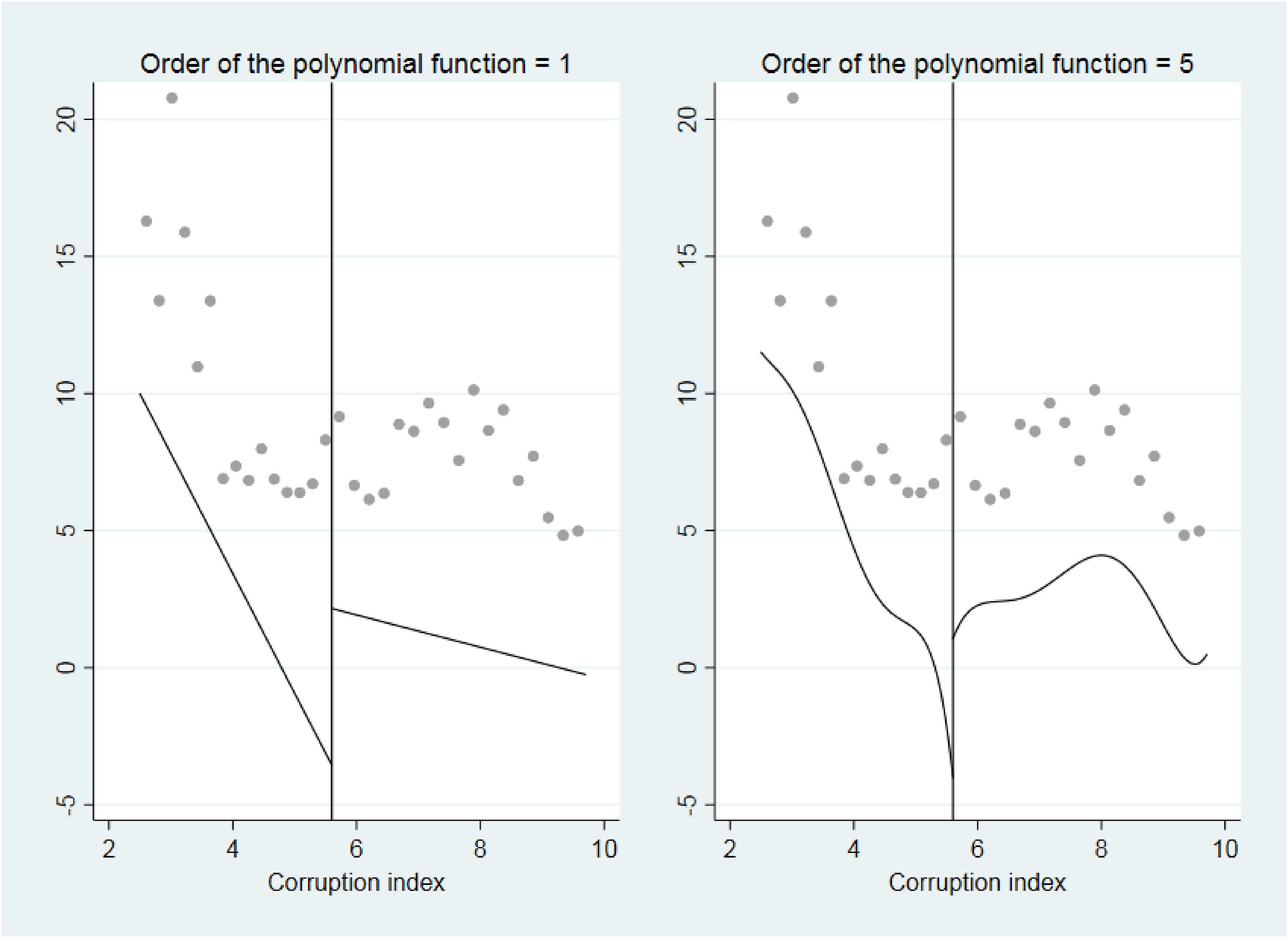
Following the recommendations of Cattaneo et al. (2019), the graphical test to detect jumps or discontinuities reports (i) two straight lines (or, alternatively, two smoothed polynomial approximations of the unknown functions) fitting the relationship between the dependent variable and the regressor of interest, before and after the identified switch point; and (ii) two non-smoothed approximations of the above unknown relationship before and after the identified switch point that proxy the local behavior of the data in the surroundings of the switch point (for technical details see Cattaneo et al., 2019). The formal test reports a point estimate of the vertical distance between the two straight lines (or the two smoothed polynomial approximations) at the switch point, together with the associated standard error and confidence interval.¹³

In sum, step 1 consists in the graphical inspection of the data. This allows for a visualization of possible nonlinearities and to check whether they result from outliers or errors. Step 2 allows for the endogenous identification of possible switch points. This enables researchers to identify switch points without making arbitrary assumptions about nonlinearity in the data. Finally, step 3 consists in a graphical inspection and a statistical test for the presence of discontinuity in the surroundings of the switch point(s) identified in step 2. This informs the researcher about the best method to deal with such switch point(s). Below, we present a replicable example and discuss the practical application of our approach in empirical management research. In the Online Supplement we provide data and Stata codes to run the whole approach, and to replicate all tables and figures included in this article.

A Replicable Illustration of the Proposed Approach

Our example exploits a cross-country dataset on the relationship between venturing and contextual variables at the macro-level. We chose this example for two main reasons. First, the data allow us to use a general topic that is well established and familiar to a broad readership. Second, all the data are publicly available and easily accessible.

Management research is placing increasing interest on contextual conditions conducive to entrepreneurial organizing. Numerous studies have found GDP per capita, unemployment rate, tax rate and inflation volatility to be systematically associated with new venture creation (see Arin et al., 2015; Busenitz et al., 2000; and Thai & Turkina, 2014, among others). Other studies, instead, have emphasized the importance of corruption, a proxy for institutional quality (see Johnson et al., 1997; and Sobel, 2008, among others). Clearly, the differences in these findings have important theoretical and practical implications. They also provide an excellent opportunity to investigate whether the presence of switch points may help us to reconcile them. Our illustrative exercise consists in testing whether including switch points will show corruption to be related to new venture creation for some range of values but not others, or to a different extent for different ranges of values.

Of course, as mentioned earlier, our theories should inform our empirical strategies. This is the case even in this exercise. We focus on corruption because, while we do not know whether a switch point may exist, nor where it may be located, institutional theory suggests that in contexts characterized by well-functioning institutions, increasing levels of perceived corruption would have a negative effect on new venture creation (Baumol, 1990). Conversely, in contexts characterized by poorly functioning institutions, perceived corruption may serve as an enabling coordination framework (albeit a costly and inefficient one) (Tonoyan et al., 2010). Taken together, these arguments suggest that the relationship between perceived corruption levels and rate of venturing may be nonlinear and change depending on institutional quality.

Importantly, our goal is not to contribute to the complex and ongoing debate on the determinants of venturing, nor to provide a theoretical contribution to our understanding of the effects of corruption on venturing. Our results are merely illustrative. These relationships are complex, broad, and well beyond the scope of this article. Instead, our goal is to provide a useful and replicable example showing that the identification of switch points produces results that differ substantially from those obtained when the possibility of their existence is ignored.

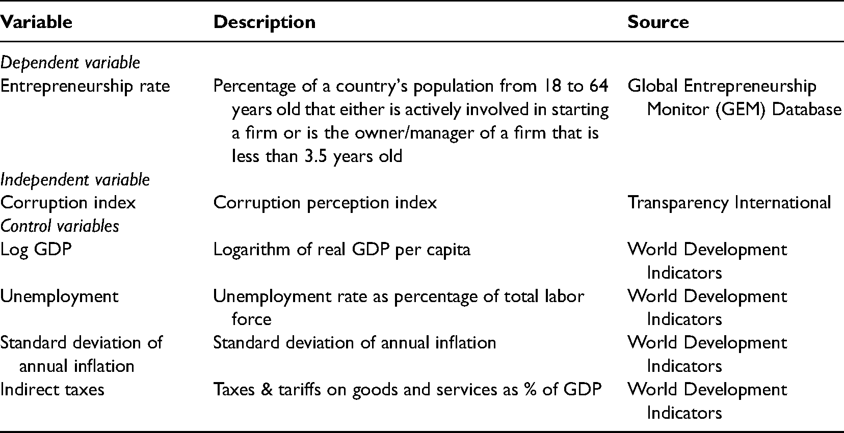
In our illustrative example, the dependent variable is the country-level rate of new venture creation (Entrepreneurship rate) obtained from the GEM database (https://www.gemconsortium.org/data). As control variables we include Log GDP, Unemployment, Standard deviation of annual inflation and Indirect taxes, obtained from the World Development Indicators (https://data.worldbank.org/products/wdi) and Transparency International (https://www.transparency.org/). Finally, we include the Corruption Perception Index (Corruption index) as independent variable and potential switch point variable.¹⁴ Table 3 provides a list and description of all variables and their sources. Since the dataset is longitudinal, each data point is a yearly observation for a specific country. Our final dataset is an unbalanced panel of 24 countries over the period 2002–2015 for a total of 281 observations.¹⁵ Table 4 shows descriptive statistics for all variables, and the pairwise correlations among them. No serious multicollinearity issues are present. We should also note that Corruption index, while not being time-invariant, shows very little variation over time for each country. This prevented us from taking full advantage of the panel structure of the data by adding fixed effects since they would be almost perfectly collinear with Corruption index. Hence, we estimated a pooled cross-sectional model.

Table 3.
Variable Descriptions and Sources.

Variable Description Source

Dependent variable

Entrepreneurship rate Percentage of a country's population from 18 to 64 years old that either is actively involved in starting a firm or is the owner/manager of a firm that is less than 3.5 years old Global Entrepreneurship Monitor (GEM) Database

Independent variable

Corruption index Corruption perception index Transparency International

Control variables

Log GDP Logarithm of real GDP per capita World Development Indicators

Unemployment Unemployment rate as percentage of total labor force World Development Indicators

Standard deviation of annual inflation Standard deviation of annual inflation World Development Indicators

Indirect taxes Taxes & tariffs on goods and services as % of GDP World Development Indicators

Table 4.
Descriptive Statistics and Pairwise Correlations.

Variable Mean S.D. (1) (2) (3) (4) (5) (6)

(1) Entrepreneurship rate 8.16 4.38 1

(2) Corruption index 6.52 2.00 −0.26* 1

(3) Log GDP 27.01 1.46 0.08 0.19* 1

(4) Unemployment 9.40 5.72 −0.13 −0.41* −0.30* 1

(5) Standard deviation of annual inflation 1171.71 3996.26 −0.00 −0.33* −0.43* 0.17* 1

(6) Indirect taxes 6.04 16.52 0.34* −0.08 −0.16* −0.16* −0.03 1

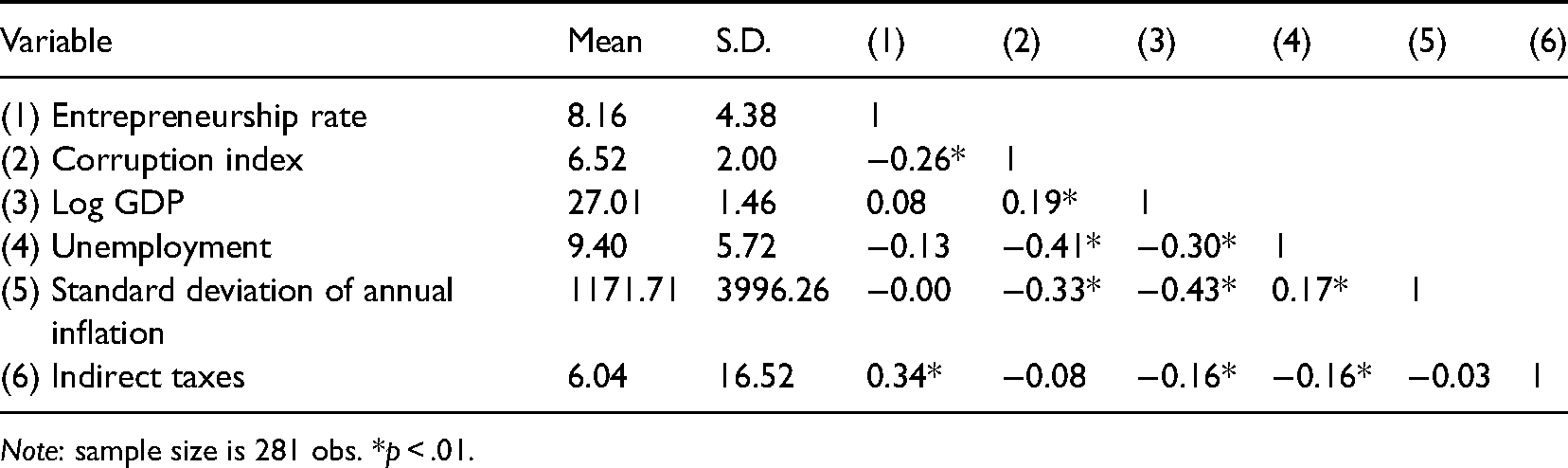
Note: sample size is 281 obs. p < .01.

Empirical Application and Results

Step One

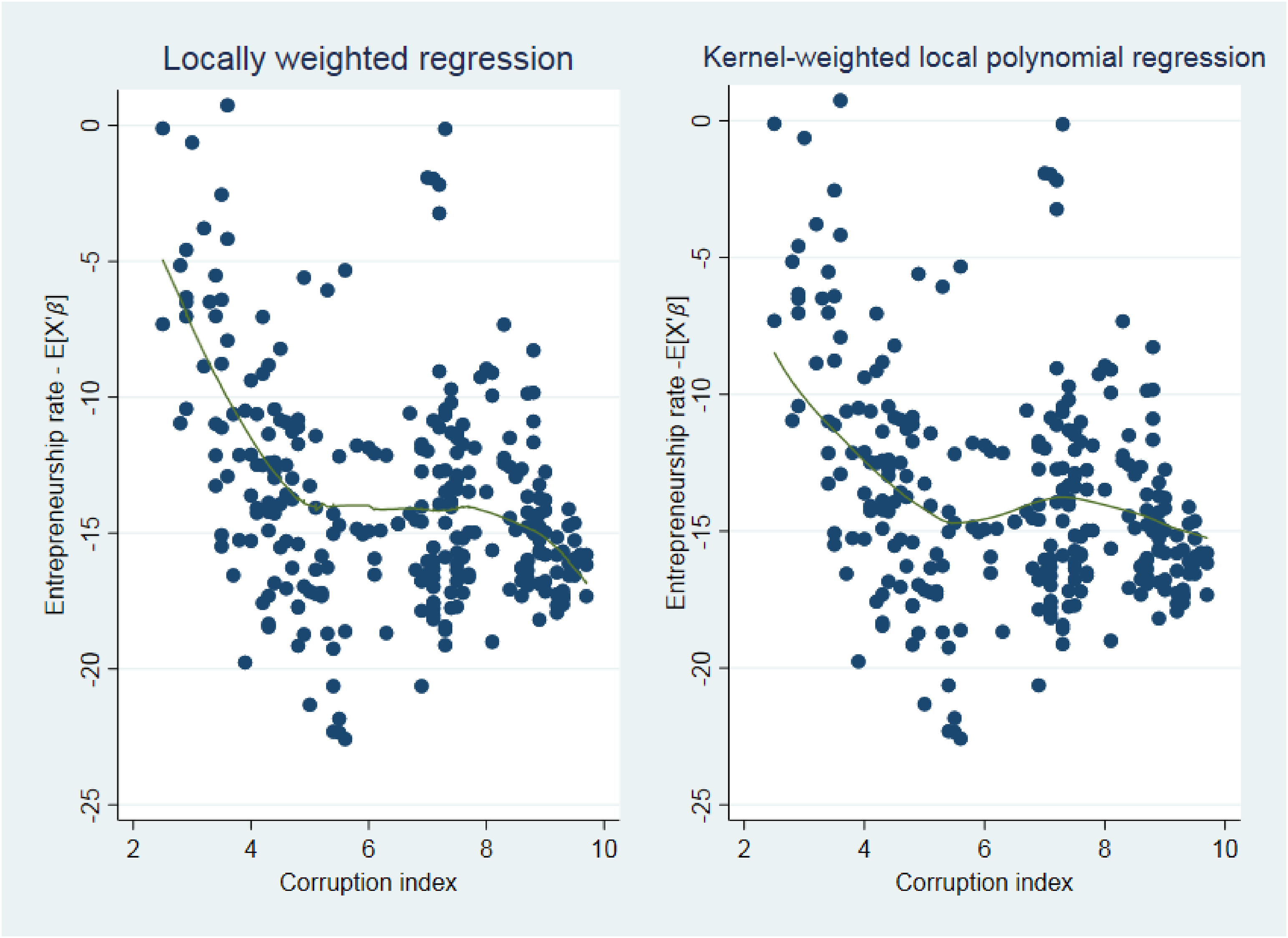
As described in the previous section, we begin by graphically inspecting our data to detect the potential presence of a switch point in the relationship between Corruption index* and Entrepreneurship rate. In the affirmative case, we then need to visualize its location over the Corruption index data range. In Figure 1 we plot the relationship between Corruption index and Entrepreneurship rate by means of both a locally weighted regression (Stata command: lowess), and a Kernel-weighted local polynomial regression (Stata command: lpoly). The figure shows that a switch point seems to be present in the surroundings of the value 5 of Corruption index.

Figure 1.
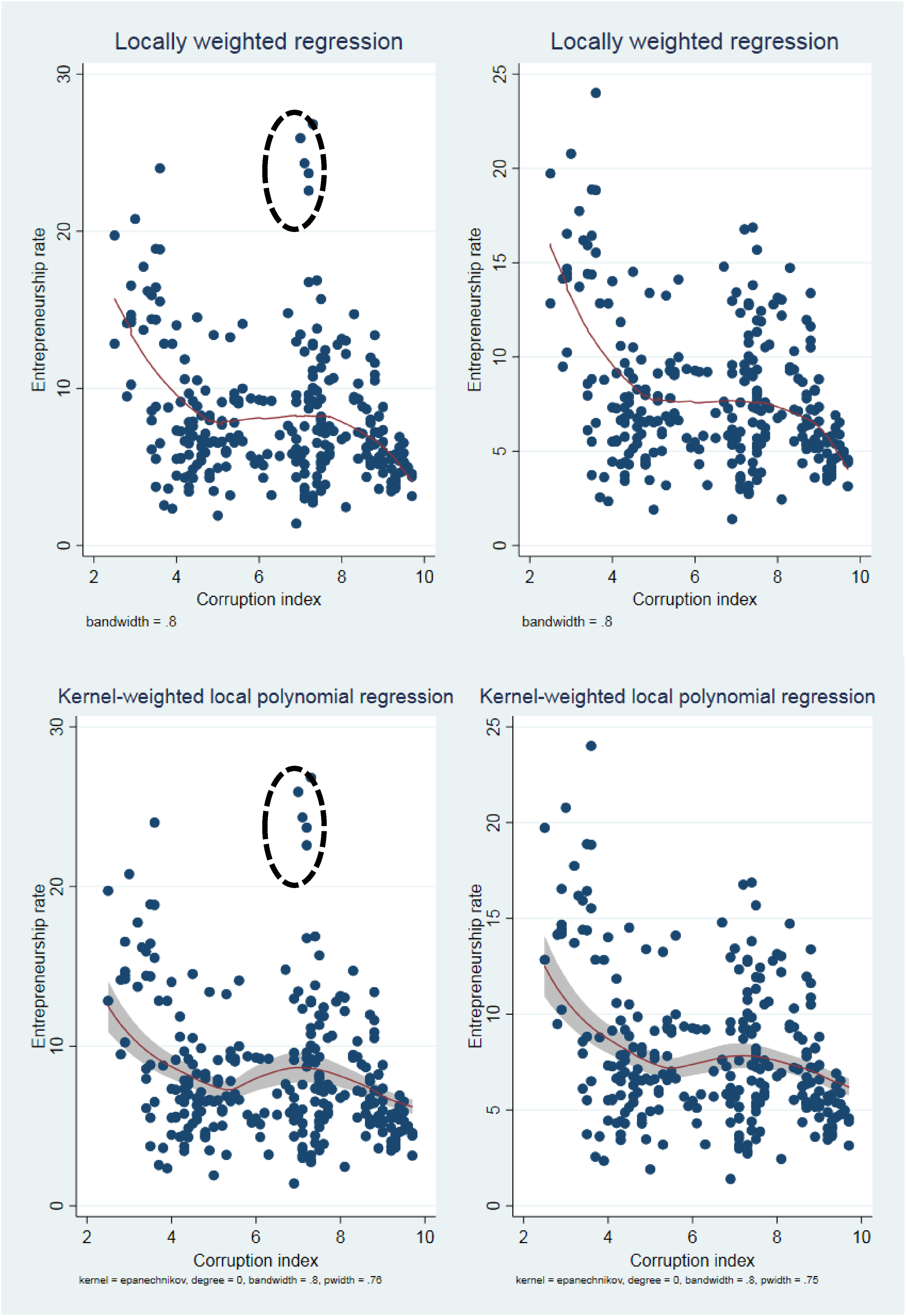
Preliminary graphical inspection of the data.

As explained earlier, this initial visual inspection provides a preliminary check for the presence of possible outliers and errors in the data, and for whether potential outliers and errors drive the identification of a switch point. Relevant errors (e.g., out of range values for Corruption index and Entrepreneurship rate) do not seem to be present in our data. However, the two panels on the left of Figure 1 showed some possible outliers identified in the dotted circles. We therefore replicated the analysis without them, and plotted the new results in the two panels on the right of Figure 1. A switch point still seems to be present in the surroundings of the value 5 of Corruption index.

Step Two

We then apply Hansen’s (2000) method and identify the switch point value formally by means of the Stata command threshold. As explained earlier, the identification of a switch point, and the value at which such switch point is located, is obtained by minimizing the SSR associated to conditional least squares estimations for all possible switch point values. Recalling Eq. (3) we have:
$\begin{aligned} E n t r e p r e n e u r s h i p r a t e = & x β + C o r r u p t i o n i n d e x δ_{1} I (0 \leq C o r r u p t i o n i n d e x < γ) \\ + C o r r u p t i o n i n d e x δ_{2} I (γ < C o r r u p t i o n i n d e x < 10) + ε; \end{aligned}$
(4)
$\begin{aligned} S S R = {E n t r e p r e n e u r s h i p r a t e - x β - C o r r u p t i o n i n d e x δ_{1} I (0 \leq C o r r u p t i o n i n d e x < γ) \\ - C o r r u p t i o n i n d e x δ_{2} I (γ < C o r r u p t i o n i n d e x < 10)}^{2}; \end{aligned}$
(5)
where x is the set of control variables (Log GDP, Unemployment, Standard deviation of annual inflation, Indirect taxes), β is the vector of coefficients for the control variables, and δ₁ and δ₂ are the coefficients for Corruption index before and after the estimated switch point, respectively. 0 and 10 represent the minimum and the maximum value that Corruption index can assume. The value of the switch point that makes SSR the smallest possible represents the value of the identified switch point.

Formally, the Stata command threshold runs a sequential estimation procedure of Equation (4) with an increasing number of switch points until it cannot reject the null hypothesis (H₀) of “no switch points.” In other words, the H₀ of “no switch points” is contrasted with the H₁ of “one switch point.” If the procedure rejects H₀ (i.e., one switch point is present in the data), then another test contrasts the new H₀ of “one switch point” with the new H₁ of “two switch points”, and so on. The procedure calculates the switch point value(s) that minimize(s) the SSR.¹⁶ When run on our data, the procedure detects only one switch point whose value is 5.6.¹⁷

A graphical representation of the identified switch point can be obtained by using the Stata command thresholdtest. This command plots a likelihood ratio (LR) test on the difference between the SSR of a linear model specification (without switch points) and the SSR of the model in Equation (4).¹⁸ In Figure 2, the LR statistic (as a function of the switch point value γ) is plotted against Corruption index; the horizontal line drawn at the value 7.35 corresponds to the asymptotical critical value at the 5% significance level (see footnote 10). Given that the LR value is below the horizontal line, this means that the null hypothesis of the LR test (i.e., no switch points) is rejected. The identified switch point is located at the minimum point of the plot, in our sample at 5.6.

Figure 2.
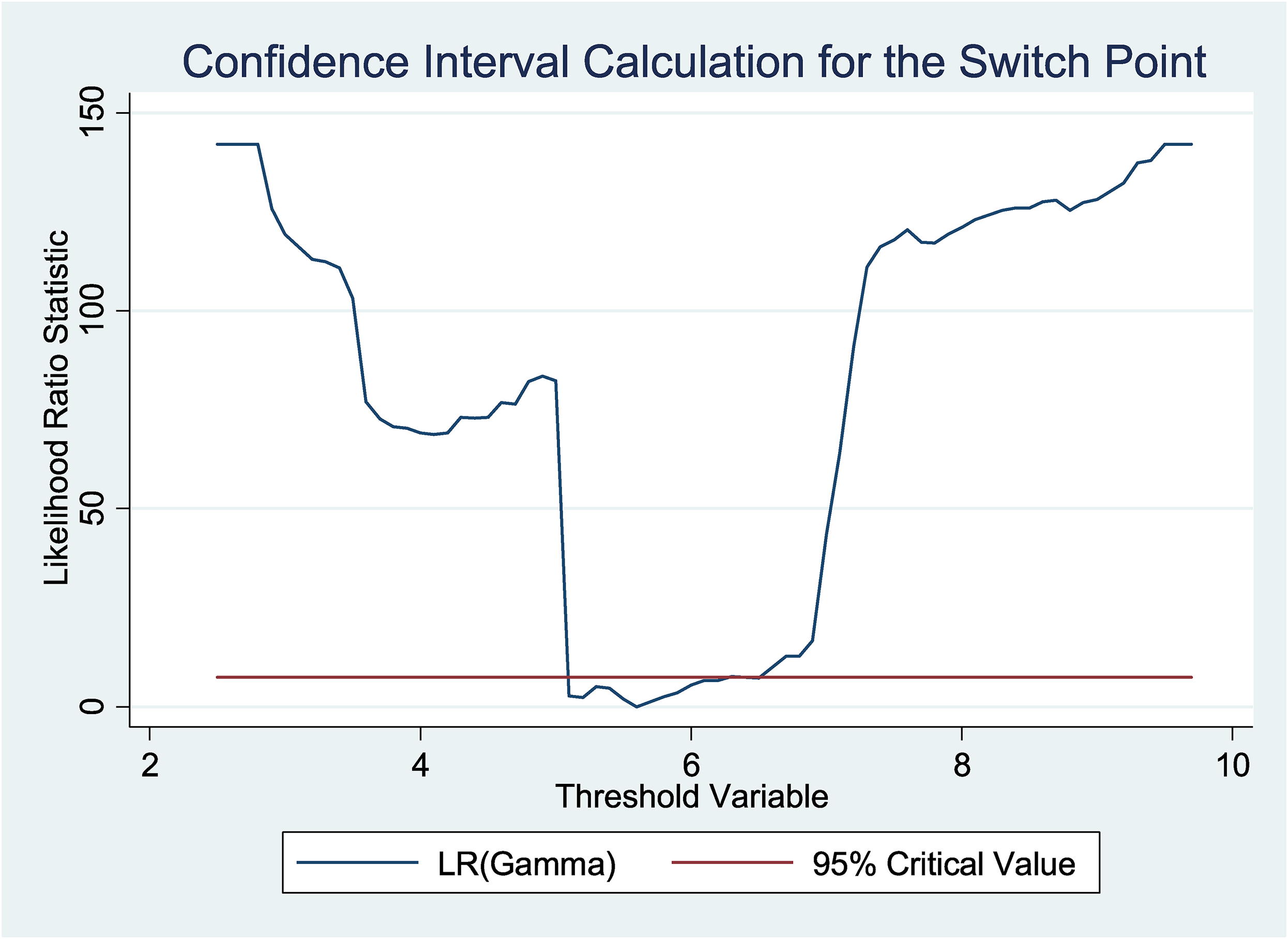
Hansen's test for corruption index.

In Table 5, the first column shows the coefficient from an OLS estimation on the whole sample, the second column shows the endogenously estimated switch point for Corruption index, and the last two columns show the estimated coefficients before and after the identified switch point. In Panel A, we estimated a model including all control variables where only the coefficient of the regressor of interest (Corruption index in this example) is allowed to vary before and after the identified switch point. In Panel B we used a more flexible specification where the coefficients of all regressors are allowed to vary before and after the identified switch point. This latter specification is the preferred specification because, in spite of being a parametric estimation method, it imposes fewer assumptions on the model specification.

Table 5.
Econometric Results.

Panel A: standard specification Coeff. whole sample Switch point Coeff. before the switch point Coeff. after the switch point

Corruption index −0.7329 5.6 −4.4186 −0.6898

(0.000) (0.000) (0.003)

SSR 3325.9904

Panel B: flexible specification Coeff. Whole Sample Switch point Coeff. before the switch point Coeff. after the switch point

Corruption index −0.7329 5.2 −4.0461 0.2820

(0.000) (0.000) (0.177)

SSR 2518.4934

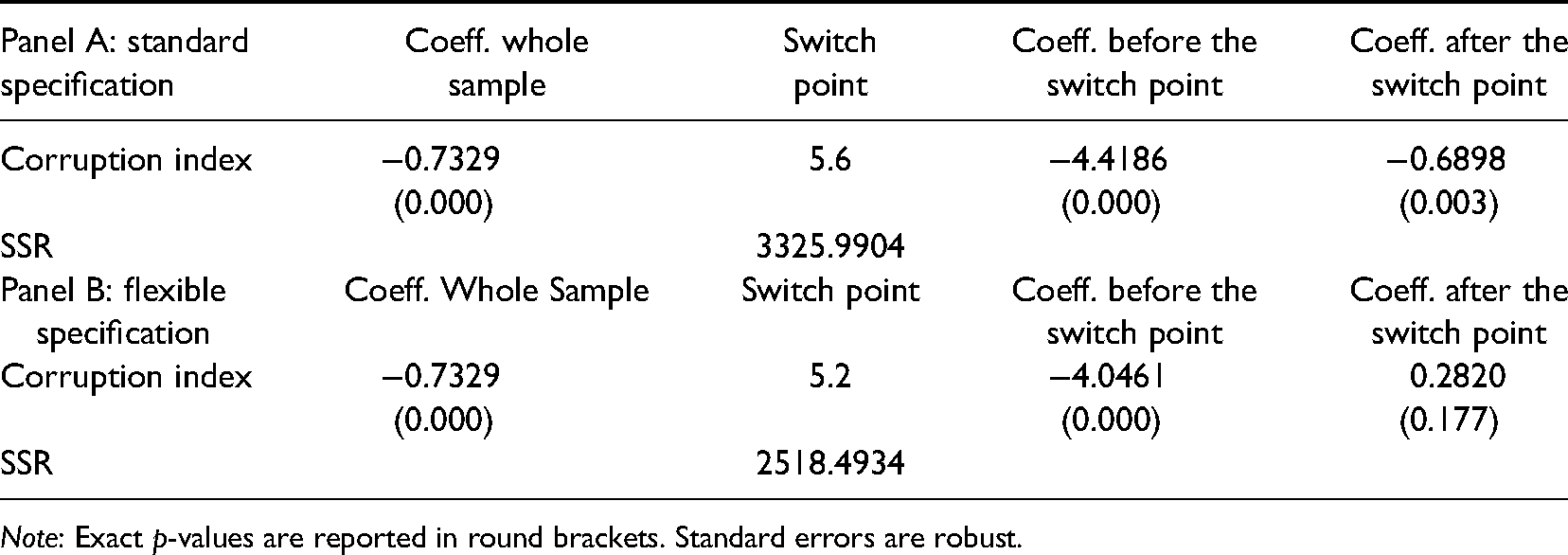
Note: Exact p-values are reported in round brackets. Standard errors are robust.

Considering that a value of Corruption index equal to zero (ten) corresponds to the highest (lowest) perceived corruption, our results indicate that, on average, a higher level of perceived corruption (i.e., a smaller coefficient of Corruption index) is positively associated with the entrepreneurship rate (first column). Interestingly, however, in Panel B this finding holds before the estimated switch point (i.e., 5.2) (third column), while the result does not hold for the subsample after the switch point (fourth column). With regard to Panel A, the estimated coefficient after the switch point is still negative but its magnitude is almost 6.5 times smaller than the one before the switch point. Consistent with our intuition, these results help reconcile previous findings. Specifically, our results suggest that in high-corruption countries more corruption is associated with more entrepreneurship, presumably because corruption may help entrepreneurs circumvent costly regulations and rent seeking (Dreher & Gassebner, 2013; Tonoyan et al., 2010). However, in less corrupt countries entrepreneurs trust more the institutional environment (Anokhin & Schulze, 2009; Baumol, 1990), and thus the corruption-enhanced coordination mechanism becomes less valuable for entrepreneurs.

Step Three

After identifying the value at which one switch point is present in the data, in Figure 3 we explore what happens in the surroundings of the identified switch point by means of a Kernel-weighted local polynomial regression. As Figure 3 shows, the identified switch point marks a change in the slope of the relationship between Entrepreneurship rate and Corruption index. However, this simple plot does not allow a proper visualization of possible discontinuities around the identified switch point. Thus, in Figure 4 and Table 6 we show a graphical test and a formal statistical test, respectively, to detect the presence of jumps or discontinuities at the switch point.

Figure 3.
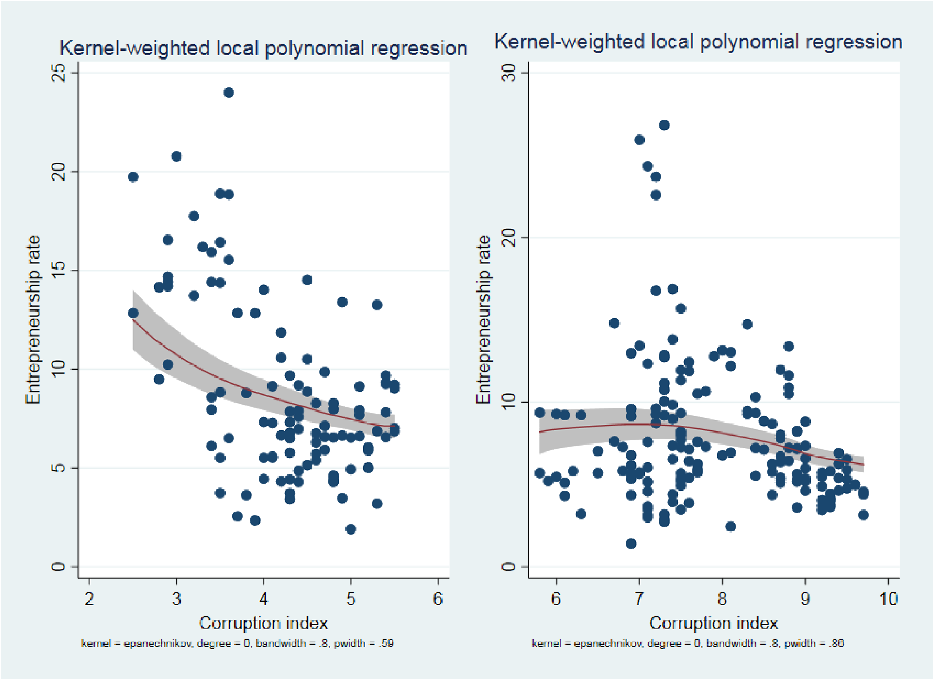
Graphical inspection of the identified switch point.

Figure 4.
Graphical inspection of the presence of discontinuities in the data around the switch point.

Table 6.
Test for Detecting Discontinuities in the Data Around the Switch Point.

Order of the polynomial function Coeff. Switch point 95% confidence interval

1 (straight line) 0.1211 5.6 [−1.52749; 1.76979]

(0.885)

5 3.3919 5.6 [−2.50341; 9.28721]

(0.259)

Note: Exact p-values are reported in round brackets. Results are robust to bias-corrected and robust bias-corrected confidence intervals.

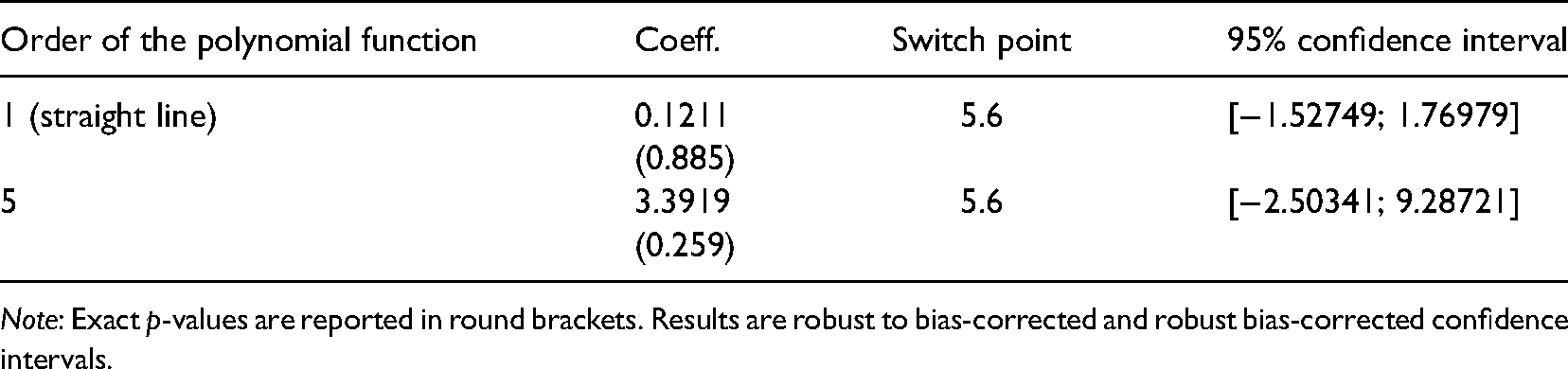
Figure 4 reports two straight lines (on the left) and two smoothed fifth-order polynomials (on the right) before and after the identified switch point (Stata command: rdplot). Even though a jump (i.e., the vertical distance between the two straight lines or the two polynomials, alternatively) seems to be there, the “local behavior” of the data (represented by the dots in the figure) in the surroundings of the switch point does not seem to highlight a discontinuity. The formal test in Table 6 (Stata command: rdrobust) reports a point estimate of the vertical distance between the two straight lines or the two smoothed polynomial approximations, alternatively, together with the associated p-value and confidence interval. As reported, both tests do not show a statistically significant discontinuity in the data at the switch point. This tells us that the use of specific methods to deal with discontinuous jumps in the data (i.e., RDD) is not required.

An Illustrative Comparison with Alternative Methods

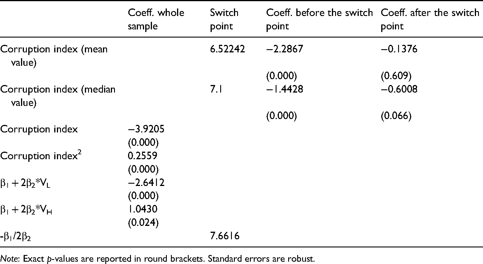
When switch points are not known a priori (as in our example), management scholars typically select those switch points on the basis of either descriptive statistics (i.e., mean, median) or U-shaped or inverted U-shaped model specifications. Table 7 shows the results obtained from applying those common practices.

Table 7.
Alternative Methods.

Coeff. whole sample Switch point Coeff. before the switch point Coeff. after the switch point

Corruption index (mean value) 6.52242 −2.2867 −0.1376

(0.000) (0.609)

Corruption index (median value) 7.1 −1.4428 −0.6008

(0.000) (0.066)

Corruption index −3.9205

(0.000)

Corruption index² 0.2559

(0.000)

β₁ + 2β₂V_L −2.6412

(0.000)

β₁ + 2β₂V_H 1.0430

(0.024)

-β₁/2β₂ 7.6616

Note: Exact p-values are reported in round brackets. Standard errors are robust.

Comparing the results in Table 7 with those in Table 5 illustrates how these common practices may fail to properly identify the real switch point value in the data. Arbitrary sample splitting at the mean or at the median is about running two separate OLS regressions on the two subsamples. In this way, all regressors’ coefficients will vary depending on how the two subsamples are constructed. In contrast, in U-shaped or inverted U-shaped model specifications, there is not sample splitting, and only one coefficient for each regressor is estimated. Thus, findings from splitting the sample at its mean or median will be compared with those in Table 5 (Panel B), while findings derived from assuming a quadratic relationship between perceived corruption and the entrepreneurship rate will be compared with those in Table 5 (Panel A).

First, when selecting the mean value of Corruption index (6.52242) in our data as the assumed (i.e., not identified) switch point, the estimated coefficient before the switch point (−2.2867) is in line (in terms of sign and statistical significance) with the one in Table 5 Panel B (−4.0461). The absolute size of the coefficient, however, is almost half the size of that in Table 5. With regard to the coefficient after the switch point (−0.1376), despite not being statistically significant, it displays an opposite sign to that in Table 5 Panel B (0.2820).

Second, when selecting the median value of Corruption index (7.1) in our data as the assumed (i.e., not identified) switch point, as in the previous case, the estimated coefficient before the switch point (−1.4428) is in line (in terms of sign and statistical significance) with the one in Table 5 Panel B (−4.0461). The absolute size of the coefficient, however, is almost three times smaller than that in Table 5. With regard to the coefficient after the switch point (−0.6008), it displays an opposite sign to that in Table 5 Panel B (0.2820) and is statistically significant (at the 10% level).

Third, we insert the squared term of Corruption index, that is, Corruption index². The coefficients of Corruption index and Corruption index² are negative (−3.9205) and positive (0.2559), respectively, and are both statistically significant. Since these coefficients may call for a U-shaped relationship, we follow guidelines from Lind and Mehlum (2010) and Haans et al. (2016) and test whether a U-shaped relationship is present in the data. Namely, we calculate the slope at the extreme values of Corruption index (the minimum and the maximum values V_L and V_H are 2.5 and 9.7, respectively), and both the slopes at V_L and V_H (given by β₁ + 2β₂V_L* and β₁ + 2β₂V_H, respectively, where β₁ and β₂ are the coefficients of Corruption index* and Corruption index²) are statistically significant and of the expected sign (i.e., negative and positive, respectively) for a U-shaped relationship. Further, the 95% confidence interval of the turning point (i.e., the potential switch point given by – β₁/2β₂) is located in the data range of Corruption index. These findings suggest a U-shaped relationship in the data, with a switch point located at the value 7.6616 of Corruption index. However, the calculated switch point is clearly quite different from the switch point identified in Table 5. Moreover, a U-shaped pattern is not in the data.

To further illustrate this point, in Figure 5 we visualize the relationship between Entrepreneurship rate and Corruption index by means of a partial dependence plot (Stata command: cprplot2). This plot shows how the dependent variable (Entrepreneurship rate) changes in response to the regressor of interest (Corruption index), conditional on inserting all other regressors (i.e., control variables) in the model (even though it is worth recalling that the choice to add the squared term of Corruption index is arbitrary). The figure still does not show a U-shape pattern in the data. In sum, arbitrarily adding a squared term to a model specification to control for possible nonlinearity does not seem to be an effective solution.

Figure 5.
Partial dependence plots for the possible presence of a quadratic relationship in the data.

Advantages and Disadvantages of the Proposed Approach

Some features of our approach need further discussion. As noted earlier, our proposed approach has several advantages in comparison to other methods. For example, it is easy to implement, and works well with small samples. Yet, there are some cases where our approach may need to be “adjusted,” or is not the preferred one and other methods should be used.

Advantages

The main advantage of our proposed approach is that it does not require researchers to make arbitrary assumptions about the shape of the relationship between variables when detecting switch points. In other words, the approach we suggest does not search in the data for what we may be looking for but checks for what is actually there. In fact, an important feature of the proposed approach is that our theoretical beliefs do not influence the results by imposing a structure on the data. Rather, the soundness of the tested theory is measured against what the data actually tell. This, however, does not mean that the approach is a-theoretical. As noted earlier, the search for switch points has to be informed by theory. Specifically, the first step of our approach forces the researcher to look through data to exclude outliers and errors that may misguide the testing process, or to identify possible nonlinear patterns that may challenge existing assumptions. The second step helps identifying possible boundaries or contingencies to existing theories. Finally, the third step informs the researcher about the type of such boundaries and contingencies, and how to deal with them. Overall, the approach we suggest provides a first line of defense against finding spurious relationships.

A further important advantage of our proposed approach is that, as mentioned earlier, it captures (that is, it statistically identifies by means of both formal statistical tests and graphical representations) all types of change (in terms of direction, magnitude or significance) in the relationship between variables. In fact, as discussed in the next paragraph, our proposed approach allows also for the identification of multiple switching points. By contrast, other methods can detect only some types of switch points (e.g., RDD), and typically only one. This feature is important because the type of switch point should guide the researcher about which method to apply for testing theory. For example, if a jump is detected (see our graphical and formal tests reported in Figure 4 and Table 6), the researcher will need to rely on theory to decide whether the conditions for an exogenous discontinuity in the probability of receiving a “treatment” are present, and, therefore a regression discontinuity method is appropriate (see Section “Dealing with switch points in management research”). If a kink is detected instead, the researcher will need to rely on theory to decide whether a regression kink model (Card et al., 2008; Hansen, 2017) can be estimated, or if a sample splitting is more appropriate.

Yet another desirable feature of our proposed approach consists in its ability to detect multiple switch points, a situation that is substantially more difficult to handle with polynomials (piecewise regressions). Specifically, the presence of further switch points can be investigated by replicating the approach sequentially for subsamples identified after the first switch point is found. The need to apply the approach sequentially is primarily because Hansen’s (1999, 2000) method only allows testing for the presence of one switch point at a time.

It is also important noting that testing for interactions in a linear model does not represent an alternative to our suggested approach. An interaction (say, positive and statistically significant) between X₁ and X₂ (where X₂ is the moderator) captures an effect such that X₂ makes the relationship between X₁ and the dependent variable more positive. In linear models, this positive moderation holds across the whole range of values. Yet, it may hold only for some portions of the distribution of X₁'s values in nonlinear models (see Hoetker, 2007 for issues on how to interpret interactions in nonlinear models). Thus, adding arbitrary interactions will only lead to the same theory testing inaccuracies mentioned above.

Finally, a more detailed comparison of the advantages of our proposed approach over supervised ML is in order, since the two methods share some characteristics. As shown in Table 2, and similarly to our proposed approach, ML methods can help researchers detect complex patterns in the relationship between Z and y (we refer to Equation (1) for simplicity). However, in their pure application, ML methods pick the functional form that best predicts y given Z and X. Thus, unlike our proposed approach, they have the disadvantage of being entirely data-driven. Although researchers can use partial dependence plots to visualize the relationship between Z and y (before using ML) to identify inconsistencies with the theory, the need to use them reduces the applicability of ML to management research.¹⁹ Indeed, patterns identified through ML preclude hypotheses from being tested on the same dataset, since doing so would amount to positing hypotheses after the results were already known. This represents a substantial cost as it requires the availability of both, a dataset where ML can be “trained,” and a main dataset where hypotheses can be tested. In sum, ML methods are best suited for situations where very large data sets are available. A luxury that, sadly, rarely applies to management research.

Disadvantages

Of course, the approach we propose has also some disadvantages. First, our approach only captures switching points for one independent variable at a time, and the identification of switch points for additional independent variables is conditional on the switching points identified in the previous round. In other words, in the presence of multiple independent variables (i.e., variables whose distribution displays a possible switch point), the researcher should prioritize independent variables and check for switch points sequentially. For instance, in our illustrative example, we could have checked for switching points in GDP or unemployment in addition to corruption. This would have required repeating our approach for each subsample identified in the previous round. Theory needs to guide the empirical analysis by informing the selection of independent variables to be tested for the presence of switch points, as well as the sequence of those tests. An example is provided by Masanjala and Papageorgiou (2004) who investigated whether the aggregate production for all countries obey a generic linear Cobb-Douglas function.

Challenging the wisdom of the time, Masanjala and Papageorgiou (2004) shifted attention toward growth nonlinearities and their relationship to variables often omitted such as literacy rates and life expectancy. They began by splitting the sample using GDP. They then used the literacy rate to identify additional switching points where the relationship between dependent and independent variables changes. Masanjala and Papageorgiou (2004) showed that, depending on the order in which independent variables are tested, countries are sorted into different groups. Thus, our advice is that, when multiple independent variables are present, and especially when theory on the relationship between the focal variables is missing or inconclusive, researchers should check the robustness of the switching points identified with our approach by repeating the analysis for different sequences of the independent variables.

Second, the number of statistically significant switch points is at least partially dependent on the sample size (due to statistical power). It is possible for a distribution of values to have multiple switch points whose interpretability and practical contribution decrease as the number of switch points increases. There is not much that can be done about that. In addition, depending on the number of regressors and the sample size, the process may be convoluted and could lead to p-hacking. This is why, as we argued above, the investigation of relevant switch points should be informed by theory. Theory allows us to dig into “suspected” switch points and to check for the presence of errors and outliers (see also the graphical inspection we propose in Figure 1). If outliers and errors are not formally detected, an “unexpected” switch point can help the researcher to build on existing theory and enrich it (or propose a new theory), perhaps via an inductive approach (i.e., Locke 2007, Shepherd & Sutcliffe, 2011).

Third, some empirical papers in management use panel data with discrete time settings, such as in the case of survival analyses (e.g., Cumming et al., 2017). In these applications, the dependent variable is the hazard rate of a certain event (e.g., a positive exit outcome or a liquidation after a venture capital investment). In other words, it is the likelihood that the event happens at time t conditional that it did not happen till t−1. For these cases, Cox-type or parametric survival models are typically used. In other applications, multiple events are modelled in a competing risk scenario. That is, a multinomial logit model is typically used where the dependent variable is categorical (one value for each competing event). To the best of our knowledge, our approach (and Hansen's method) is not applicable.

Fourth, as explained in section “Switch points in management research,” if a natural dichotomization is present in the data (i.e., the switch point variable is dichotomous), the proposed approach is irrelevant. Fifth, the second step of our approach assumes that possible nonlinearities (i.e., switch points) in linear models are explained by observable variables, even though the number of switch points and their identified values are not known ex ante. When theory suggests that nonlinearities are driven by latent (i.e., not observable) variables, Markov switching models are a preferred method to our approach (Chan et al., 2017).

Extensions of our Approach

Some extensions to step 2 in our approach have been recently developed. While a detailed survey of these extensions is beyond the scope of this article, some of them can be useful for management scholars. First, an extended threshold model (here we use the terminology of Qian et al., 2018) allows the possibility to include a censored regressor (i.e., a regressor subject to random censoring) in a linear regression model specification. Second, when the dependent variable is a count (following, for instance, a Poisson or a negative binomial distribution), the researcher can apply the logarithmic transformation to the dependent variable and still run the second step of our proposed approach. Third, when using panel data, a fixed effects panel version of the second step of our approach is available (Wang, 2015; Stata command: xthreg). This panel estimator, however, is static and does not establish causality, nor controls for endogeneity (indeed, it requires strong exogeneity of regressors). Seo and Shin (2016) have extended this estimator to a dynamic version (where the lagged dependent variable can be included) with potentially endogenous switch point variables and regressors. This dynamic version can be estimated by means of the Generalized Method of Moments (GMM) method (Seo et al., 2019; Stata command: xthenreg).²⁰

Discussion and Recommendations for Authors

Although switch points are often implicitly included in management research, their presence in the data is either ignored, or tested with arbitrarily specified functional forms or procedures. This is problematic if we want accurate tests for our theories. In fact, when switch points are properly accounted for, some relationships validated empirically with linear methods may be found to display coefficients that, based on the reference sample, change in sign, magnitude, and generalizability over the variable range. These issues are particularly relevant in management research where validating previous empirical evidence is often the starting point for developing new research questions.

Importantly, the approach described in this paper has broad applicability across management domains and it is useful in addressing several open questions. Here we provide some indicative examples. First, research on the behavioral theory of the firm suggests that a balance between exploration and exploitation in problemistic searches is necessary to maximize a firm's performance (e.g., Gupta et al., 2006). As argued by March (1991), too much attention dedicated to exploration activities may lead to a risky allocation of scarce resources. Too much exploitation, however, may reduce the organization's ability to adapt to environmental shocks. Indeed, scholars have found evidence of an inverted U-shaped relationship between the relative share of explorative activities and firm performance (Uotila et al., 2009). These results, however, are contingent upon the adoption of a quadratic model specification. Should the relationship in the data be other than quadratic, our beliefs about the slope and significance of the relationship may not hold. The approach we suggest may help us to calibrate the tradeoff between exploration and exploitation and contribute to our understanding of problemistic searches.

Second, research in leadership and organizational behavior shows leadership influence and effectiveness to exhibit nonlinear relationships with several variables. Antonakis et al. (2017), for example, have found that the relation between IQ and perceived leadership might be more accurately described by a curvilinear than a linear function. Lam et al. (2015) have found participative leadership to be unrelated to employee performance before a certain switch point, but to be associated to higher employee performance after that switch point. Similarly, Maruping et al. (2015) have found the relationship between time pressure and team leadership performance to be non-linear. In all these cases, the presence and shape of the non-linearity was tested using mediating effects. The estimated coefficients, however, rest on researcher-defined equations and, often, small sample sizes. Our proposed approach may help researchers to verify whether some long held theoretical beliefs hold when tested without relying on functional forms selected arbitrarily.

Third, research in organizational behavior shows the relationship between accountability and job tension to be positive and linear for individuals with high negative affectivity (NA) but non-linear for individuals with low NA (Hochwarter et al., 2005). However, as the authors acknowledge, these results may be somewhat dependent on sample sizes. In fact, while tracing evidence for non-monotonic effects in several psychology applications, Grant and Schwartz (2011, p.71) note “given the apparent pervasiveness of non-monotonic effects, a good rule of thumb for study design may be to include a wide enough range of values of the independent variable to enable a judgment of when non-monotonicity occurs rather than whether non-monotonicity occurs.” As we have shown, however, this “judgment,” albeit informed by theory, may be nonetheless inaccurate or biased. Our approach enables researchers to resolve this problem.

Fourth, research on top management teams (TMTs) has extensively investigated the impact of TMT diversity on firm performance. TMT diversity is likely conducive to a more effective problem-solving process within the team (van Dijk et al., 2017). As argued by upper-echelons research (Hambrick, 2007), diversity is a proxy for different beliefs, values and attitudes that may lead to different corporate behaviors and to decisions of a better quality (Keck & Tang, 2017). Yet, TMT diversity could also have negative or negligible effects on firm performance. For example, conflicts within the team may be more likely to emerge in diverse teams due to divergence in goal congruence and shared knowledge (Jehn et al., 1999). Indeed, focusing on the effect of TMT diversity on firm internationalization, scholars have found that tenure diversity has a positive impact on firm internationalization, while education diversity has a negligible effect (Barkema & Shvyrkov, 2007). The approach we suggest would help researchers to investigate whether these effects hold for the whole sample, and when alternative measures of diversity (e.g., experience, education, age) are considered.

Fifth, research in strategic management investigates tradeoffs associated with the decision to internalize or outsource activities to improve firm performance (e.g., Leiblein et al., 2002). While internalization through vertical integration allows firms to economize on transaction costs (Williamson, 1975), strategic outsourcing fosters organization flexibility and access to external knowledge (Powell et al., 1996). Indeed, Rothaermel et al. (2006) have introduced the concept of taper integration, i.e., the simultaneous pursuit of vertical integration (VI) and strategic outsourcing (SO). From a methodological standpoint, this tension is captured by including in the analysis both the linear and quadratic terms for VI and SO, and the interaction of the linear terms. As in the case of team diversity, it would be informative to test whether these relationships are stable over the whole range of the variables’ values.

These are, of course, just a few examples of the large and diverse areas of inquiry that could benefit from using the approach we propose. A list of all possible applications is beyond the scope of this article and, perhaps, impossible. Yet, we hope these examples will resonate with scholars working across a broad spectrum of management research, and encourage them to incorporate the investigation of endogenous switch points in their work.

Conclusion

Extant research has shown the theoretical and empirical perils of dealing with unknown potential limitations in the data, and in existing statistical methods (Dul, 2016; Ostroff, 1993; Rönkkö et al., 2021). Within this context, we provide an integrative framework for the identification of nonlinearities that constitutes a precursor step that researchers will want to conduct to subsequently make better decisions about an appropriate model specification and estimation method (e.g., quadratic terms vs. split samples, etc.). Adding this best practice to our work may significantly improve the explanatory power of our empirical models. As scholars, we should strive to include in our work methods that increase the soundness of our results. This is particularly important at a time when our theories can make a difference in people's lives and yet their relevance is increasingly called into question.

Supplemental Material

sj-dta-1-orm-10.1177_10944281211058466 - Supplemental material for Inflection Points, Kinks, and Jumps: A Statistical Approach to Detecting Nonlinearities

Supplemental material, sj-dta-1-orm-10.1177_10944281211058466 for Inflection Points, Kinks, and Jumps: A Statistical Approach to Detecting Nonlinearities by Peren Arin, Maria Minniti, Samuele Murtinu and Nicola Spagnolo in Organizational Research Methods

Supplemental Material

sj-do-2-orm-10.1177_10944281211058466 - Supplemental material for Inflection Points, Kinks, and Jumps: A Statistical Approach to Detecting Nonlinearities

Supplemental material, sj-do-2-orm-10.1177_10944281211058466 for Inflection Points, Kinks, and Jumps: A Statistical Approach to Detecting Nonlinearities by Peren Arin, Maria Minniti, Samuele Murtinu and Nicola Spagnolo in Organizational Research Methods

Graphical illustrations	Definition	Implications
Panel A: Inflection points
	An inflection point is a switch point on a continuous function where a change in the direction of the curvature occurs	Statistical significance exists before and/or after the switch point

Panel B: Kinks
	A kink is a switch point on a continuous function where both sides are straight lines	Statistical significance may exist only before or after the kink (top plots) or before and after the kink (bottom plots)

Panel C: Jumps
	A jump is a switch point that identifies a discontinuity in a function	Statistical significance may or may not exist before and/or after the jump
Panel D: Multiple switch points
	Functions may exhibit combinations of two or more switch points, of similar or different types	Statistical significance may exist before and/or after each switch point, depending on the type of each switch point

Method	Description	Example reference
Piecewise regression	Method to define whether a certain number of (linear) relationships fits the data better than one relationship	Lovallo et al. (2020)
Nonlinear curve fitting	Method that searches the best fit with the data of a researcher-defined equation	Shafer et al. (2001)
Test for structural breaks in time series	Wald and likelihood ratio tests to detect a structural change in mean in a time series	Trebbi and Xiao (2019)
Regression tree analysis	Method for the identification of higher order interdependencies between variables	Durlauf and Johnson (1995)
Arbitrary split sample	Method to split the sample on the basis of descriptive statistics (e.g., mean, median)	Kogut et al. (2014)
Arbitrary addition of polynomial terms	Method to augment a regression with polynomial terms (e.g., squared term of the independent variable)	Karim (2009)
Supervised machine learning (ML)	Method to detect complex relationships in the data	Choudhury et al. (2021)
Regression discontinuity design	Quasi-experimental design used to estimate treatment effects when there is a discontinuity (known ex ante) in the probability of receiving treatment	Bradley et al. (2017)

Variable	Description	Source
Dependent variable
Entrepreneurship rate	Percentage of a country's population from 18 to 64 years old that either is actively involved in starting a firm or is the owner/manager of a firm that is less than 3.5 years old	Global Entrepreneurship Monitor (GEM) Database
Independent variable
Corruption index	Corruption perception index	Transparency International
Control variables
Log GDP	Logarithm of real GDP per capita	World Development Indicators
Unemployment	Unemployment rate as percentage of total labor force	World Development Indicators
Standard deviation of annual inflation	Standard deviation of annual inflation	World Development Indicators
Indirect taxes	Taxes & tariffs on goods and services as % of GDP	World Development Indicators

Variable	Mean	S.D.	(1)	(2)	(3)	(4)	(5)	(6)
(1) Entrepreneurship rate	8.16	4.38	1
(2) Corruption index	6.52	2.00	−0.26*	1
(3) Log GDP	27.01	1.46	0.08	0.19*	1
(4) Unemployment	9.40	5.72	−0.13	−0.41*	−0.30*	1
(5) Standard deviation of annual inflation	1171.71	3996.26	−0.00	−0.33*	−0.43*	0.17*	1
(6) Indirect taxes	6.04	16.52	0.34*	−0.08	−0.16*	−0.16*	−0.03	1

Panel A: standard specification	Coeff. whole sample	Switch point	Coeff. before the switch point	Coeff. after the switch point
Corruption index	−0.7329	5.6	−4.4186	−0.6898
	(0.000)		(0.000)	(0.003)
SSR		3325.9904
Panel B: flexible specification	Coeff. Whole Sample	Switch point	Coeff. before the switch point	Coeff. after the switch point
Corruption index	−0.7329	5.2	−4.0461	0.2820
	(0.000)		(0.000)	(0.177)
SSR		2518.4934

Order of the polynomial function	Coeff.	Switch point	95% confidence interval
1 (straight line)	0.1211	5.6	[−1.52749; 1.76979]
	(0.885)
5	3.3919	5.6	[−2.50341; 9.28721]
	(0.259)

Footnotes

Acknowledgment

The authors are grateful to Kemal Kivanc Akoz, Olivia Cassero, Nicolina Kamenou-Aigbekaen, and Murat Koyuncu for their suggestions and Senad Lekpek for research assistance.

Declaration of Conflicting Interests

The authors declared no potential conflicts of interest with respect to the research, authorship, and/or publication of this article.

Funding

The authors received no financial support for the research, authorship and/or publication of this article.

ORCID iDs

Peren Arin

Samuele Murtinu

Supplemental material

Supplemental material for this article is available online.

Notes

Author biographies

Peren Arin holds a PhD in Economics from Louisiana State University. He is currently a Professor at Zayed University, a Research Associate at the Centre of Applied Macroeconomic Analysis at Australian National University, and an associate editor of Springer Nature: Business & Economics.

Maria Minniti holds a PhD in Economics from New York University. She is currently Professor and Louis A. Bantle Endowed Chair of Entrepreneurship and Public Policy at the Whitman School of Management, and the Director of the Institute for an Entrepreneurial Society (IES) at Syracuse University.

Samuele Murtinu holds a PhD in Management, Economics and Industrial Engineering from Politecnico di Milano. He is currently a Professor of International Business at Utrecht University School of Economics.

Nicola Spagnolo holds a Ph.D. in Economics from the University of London. He is currently a Professor at Brunel University London, and a Research Associate with the Centre for Applied Macroeconomic Analysis at Australian National University, and with Universita’ degli Studi della Campania “Luigi Vantivelli.”

References

Agarwal

Croson

Mahoney

J. T

. (2010). The role of incentives and communication in strategic alliances: An experimental investigation. Strategic Management Journal, 31(4), 413–437. https://doi.org/10.1002/sej.96

Aguinis

Gottfredson

R.K.

Joo

. (2013) Best-Practice recommendations for defining, identifying, and handling outliers. Organizational Research Methods, 16(2), 270–301. https://doi.org/10.1177/1094428112470848

Amore

M. D.

Murtinu

. (2021). Tobit models in strategy research: Critical issues and applications. Global Strategy Journal, 11(3), 331-355. https://doi.org/10.1002/gsj.1363.

Andrews

D. W.

Ploberger

. (1994). Optimal tests when a nuisance parameter is present only under the alternative. Econometrica, 62(6), 1383–1414. https://doi.org/10.2307/2951753

Anokhin

Schulze

W. S

. (2009). Entrepreneurship, innovation, and corruption. Journal of Business Venturing, 24(5), 465–476. https://doi.org/10.1016/j.jbusvent.2008.06.001

Antonakis

House

R.J.

Simonton

. (2017). Can super smart leaders suffer from too much of a good thing? The curvilinear effect of intelligence on perceived leadership behavior. Journal of Applied Psychology, 102(7), 1003–1021. https://doi.org/10.1037/apl0000221

Arin

K. P.

Huang

V. Z.

Minniti

Nandialath

A. M.

Reich

O. F

. (2015). Revisiting the determinants of entrepreneurship: A Bayesian approach. Journal of Management, 41(2), 607–631. https://doi.org/10.1177/0149206314558488

Barkema

H. G.

Shvyrkov

. (2007). Does top management team diversity promote or hamper foreign expansion? Strategic Management Journal, 28(7), 663–680. https://doi.org/10.1002/smj.604

Baumol

W.J

. (1990). Entrepreneurship: Productive, unproductive, and destructive. Journal of Political Economy, 98(5–1), 893–921. https://doi.org/10.1086/261712

10.

Bowen

H.P

. (2012). Testing moderating hypotheses in limited dependent Variable and other nonlinear models: Secondary versus total interactions. Journal of Management, 38(3), 860–889. https://doi.org/10.1177/0149206309356324

11.

Bradley

Kim

Tian

. (2017). Do unions affect innovation? Management Science, 63(7), 2251–2271. https://doi.org/10.1287/mnsc.2015.2414

12.

Bruton

G. D.

Filatotchev

Chahine

Wright

. (2010). Governance, ownership structure, and performance of IPO firms: The impact of different types of private equity investors and institutional environments. Strategic Management Journal, 31(5), 491–509. https://doi.org/10.1111/j.1540-6520.2010.00390.x

13.

Busenitz

L. W.

Gomez

Spencer

J. W

. (2000). Country institutional profiles: Unlocking entrepreneurial phenomena. Academy of Management Journal, 43(5), 994–1003. https://doi.org/10.2307/1556423

14.

Caner

Hansen

B. E

. (2004). Instrumental variable estimation of a threshold model. Econometric Theory, 20(5), 813–843. https://doi.org/10.1017/S0266466604205011

15.

Card

Mas

Rothstein

. (2008). Tipping and the dynamics of segregation. The Quarterly Journal of Economics, 123(1), 177–218. https://doi.org/10.1162/qjec.2008.123.1.177

16.

Cattaneo

M. D.

Idrobo

Titiunik

(2019). A practical introduction to regression discontinuity designs: Foundations. Cambridge University Press.

17.

Certo

Sirmon

D.G.

Brymer

R.A

. (2010). Competition and scholarly productivity in management: Investigating changes in scholarship from 1988 to 2008. Academy of Management Learning and Education, 9(4):591–606. https://doi.org/10.5465/amle.9.4.zqr591

18.

Chan

K. S.

Hansen

B. E.

Timmermann

(2017). Guest Editors’ Introduction: Regime switching and threshold models. Journal of Business & Economic Statistics, 35(2), 159–161. https://doi.org/10.1080/07350015.2017.1236521

19.

Chatain

. (2011). Value creation, competition, and performance in buyer-supplier relationships. Strategic Management Journal, 32(1), 76–102. https://doi.org/10.1002/smj.864

20.

Choudhury

Allen

R. T.

Endres

M. G

. (2021). Machine learning for pattern discovery in management research. Strategic Management Journal, 42(1), 30–57 https://doi.org/10.1002/smj.3215

21.

Cumming, D. J., Grilli, L., & Murtinu, S. (2017). Governmental and independent venture capital investments in Europe: A firm-level performance analysis. Journal of Corporate Finance, 42, 439-459.

22.

Davies

R. B

. (1977). Hypothesis testing when a nuisance parameter is present only under the alternative. Biometrika, 64(2), 247–254. https://doi.org/10.2307/2335690

23.

Davies

R. B

. (1987). Hypothesis testing when a nuisance parameter is present only under the alternative. Biometrika, 74(1), 33–43. https://doi.org/10.2307/2336019

24.

Dezsö

C. L.

Ross

D. G

. (2012). Does female representation in top management improve firm performance? A panel data investigation. Strategic Management Journal, 33(9), 1072–1089. https://doi.org/10.1002/smj.1955

25.

Dreher

Gassebner

. (2013). Greasing the wheels? The impact of regulations and corruption on firm entry. Public Choice, 155(3–4), 413–432. https://doi.org/10.1007/s11127-011-9871-2

26.

Dul

. (2016). Necessary condition analysis (NCA): Logic and methodology of “necessary but Not sufficient” causality. Organizational Research Methods, 19(1), 10–52 https://doi.org/10.1177/1094428115584005

27.

Durlauf

S. N.

Johnson

P. A

. (1995). Multiple regimes and cross-country growth behavior. Journal of Applied Econometrics, 10(4), 365–384. https://doi.org/10.1002/jae.3950100404

28.

Fan

Heckman

N. E.

Wand

M. P

. (1995). Local polynomial kernel regression for generalized linear models and quasi-likelihood functions. Journal of the American Statistical Association, 90(429), 141–150. https://doi.org/10.1080/01621459.1995.10476496

29.

Finkelstein

. (2009). The effects of strategic and market complementarity on acquisition performance: Evidence from the US commercial banking industry, 1989–2001. Strategic Management Journal, 30(6), 617–646. https://doi.org/10.1002/smj.754

30.

Flammer

. (2015). Does product market competition foster corporate social responsibility? Evidence from trade liberalization. Strategic Management Journal, 36(10), 1469–1485. https://doi.org/10.1002/smj.2307

31.

Foss

Lee

P. M.

Murtinu

Scalera

V. G

. (2021). The XX factor: Female managers and innovation in a cross-country setting. The Leadership Quarterly. https://doi.org/10.1016/j.leaqua.2021.101537

32.

Gibbert

Nair

L. B.

Weiss

Hoegl

. (2021). Using outliers for theory building. Organizational Research Methods, 24(1), 172–181. https://doi.org/10.1177/1094428119898877

33.

Gonzalo

Pitarakis

J. Y

. (2002). Estimation and model selection based inference in single and multiple threshold models. Journal of Econometrics, 110(2), 319–352. https://doi.org/10.1016/S0304-4076(02)00098-2

34.

Grant

A.M.

Schwartz

. (2011). Too much of a good thing: The challenge and opportunity of the inverted U. Perspectives on Psychological Science, 6(1) 61–76 https://doi.org/10.1177/1745691610393523

35.

Greve

H. R

. (2003). A behavioral theory of R&D expenditures and innovations: Evidence from shipbuilding. Academy of Management Journal, 46(6), 685–702. https://doi.org/10.5465/30040661

36.

Gupta

A. K.

Smith

K. G.

Shalley

C. E

. (2006). The interplay between exploration and exploitation. Academy of Management Journal, 49(4), 693–706. https://doi.org/10.5465/amj.2006.22083026

37.

Haans

R. F.

Pieters

Z. L

. (2016). Thinking about U: Theorizing and testing U-and inverted U-shaped relationships in strategy research. Strategic Management Journal, 37(7), 1177–1195. https://doi.org/10.1002/smj.2399

38.

Hahn

Todd

Van der Klaauw

. (2001). Identification and estimation of treatment effects with a regression-discontinuity design. Econometrica, 69(1), 201–209. https://doi.org/10.1111/1468-0262.00183

39.

Hambrick

D. C

. (2007). Upper echelons theory: An update. Academy of Management Review, 32(2), 334–343. https://doi.org/10.5465/amr.2007.24345254

40.

Hansen

B. E

. (1992). The likelihood ratio test under nonstandard conditions: Testing the markov switching model of GNP. Journal of Applied Econometrics, 7(S1), S61–S82. https://doi.org/10.1002/jae.3950070506

41.

Hansen

B. E

. (1996). Inference when a nuisance parameter is not identified under the null hypothesis. Econometrica, 64(2), 413–430. https://doi.org/10.2307/2171789

42.

Hansen

B. E

. (1999). Threshold effects in non-dynamic panels: Estimation, testing, and inference. Journal of Econometrics 93(2), 345–368. https://doi.org/10.1016/S0304-4076(99)00025-1

43.

Hansen

B. E

. (2000). Sample splitting and threshold estimation. Econometrica, 68(3), 575–603. https://doi.org/10.1111/1468-0262.00124

44.

Hansen

B. E

. (2017). Regression kink with an unknown threshold. Journal of Business & Economic Statistics, 35(2), 228–240. https://doi.org/10.1080/07350015.2015.1073595

45.

Heeley

M.B.

Jacobson

. (2008). The recency of technological inputs and financial performance. Strategic Management Journal, 29(7), 723–744. https://doi.org/10.1002/smj.682

46.

Hochwarter

W.A.

Perrewé

Hall

A.T.

Ferris

G.R

. (2005) Negative affectivity as a moderator of the form and magnitude of the relationship between felt accountability and job tension. Journal of Organizational Behavior, 26(5), 517–534. https://doi.org/10.1002/job.324

47.

Hoetker

. (2007). The use of logit and probit models in strategic management research: Critical issues. Strategic Management Journal, 28(4), 331–343. https://doi.org/10.1002/smj.582

48.

Huselid

Day

N.E

. (1991). Organizational commitment, Job involvement, and turnover: A substantive and methodological analysis. Journal of Applied Psychology, 76(3), 380–396. https://doi.org/10.1037/0021-9010.76.3.380

49.

Jehn

K. A.

Northcraft

G. B.

Neale

M. A

. (1999). Why differences make a difference: A field study of diversity, conflict and performance in workgroups. Administrative Science Quarterly, 44(4), 741–763. https://doi.org/10.2307/2667054

50.

Johnson

Kaufmann

Shleifer

. (1997). The unofficial economy in transition. Brookings Papers on Economic Activity, 1997(2) 159–239. https://doi.org/10.2307/2534688

51.

Karim

. (2009). Business unit reorganization and innovation in new product markets. Management Science, 55(7), 1237–1254. https://doi.org/10.1287/mnsc.1090.1017

52.

Keck

Tang

. (2017). Gender composition and group confidence judgment: The perils of all-male groups. Management Science, 64(12), 5877–5898. https://doi.org/10.1287/mnsc.2017.2881

53.

Kogut

Colomer

Belinky

. (2014). Structural equality at the top of the corporation: Mandated quotas for women directors. Strategic Management Journal, 35(6), 891–902. https://doi.org/10.1002/smj.2123

54.

Lam

C.K.

Huang

Chan

S.C

. (2015). The threshold effect of participative leadership and the role of leader information sharing. Academy of Management Journal, 58(3), 836–855. https://doi.org/10.5465/amj.2013.0427

55.

., Robbins

S.B

., Ilies

., Holland

Westrick

. (2011) Too much of a good thing: Curvilinear relationships between personality traits and job performance. Journal of Applied Psychology, 96(1), 113 − 1132. https://doi.org/10.1037/a0021016

56.

Leiblein

M. J.

Reuer

J. J.

Dalsace

. (2002). Do make or buy decisions matter? The influence of organizational governance on technological performance. Strategic Management Journal, 23(9), 817 − 8833. https://doi.org/10.1002/smj.259

57.

Lieberman

M. B.

Lee

G. K.

Folta

T. B

. (2017). Entry, exit, and the potential for resource redeployment. Strategic Management Journal, 38(3), 526–544. https://doi.org/10.1002/smj.2501

58.

Lind

J. T.

Mehlum

. (2010). With or without U? The appropriate test for a U-shaped relationship. Oxford Bulletin of Economics and Statistics, 72(1), 109–118. https://doi.org/10.1111/j.1468-0084.2009.00569.x

59.

Locke

E. A

. (2007). The case for inductive theory building. Journal of Management, 33(6), 867–890. https://doi.org/10.1177/0149206307307636

60.

Lovallo

Brown

A. L.

Teece

D. J.

Bardolet

. (2020). Resource re-allocation capabilities in internal capital markets: The value of overcoming inertia. Strategic Management Journal, 41(8),1365–1380. https://doi.org/10.1002/smj.3157

61.

Maruping

L. M

., Venkatesh,

., Thatcher

., & Patel

P.C

. (2015). folding under pressure or rising to the occasion? Perceived time pressure and the moderating role of team temporal leadership. Academy of Management Journal, 58(5), 1313–1333. https://doi.org/10.5465/amj.2012.0468

62.

March

J. G

. (1991). Exploration and exploitation in organizational learning. Organization Science, 2(1), 71–87. https://doi.org/10.1287/orsc.2.1.71

63.

Masanjala

W.H.

Papageorgiou

. (2004). The solow model with CES technology: Nonlinearities and parameter heterogeneity. Journal of Applied Econometrics, 19(2), 171–201. https://doi.org/10.1002/jae.722

64.

Miller

K. D.

Chen

W. R

. (2004). Variable organizational risk preferences: Tests of the march-shapira model. Academy of Management Journal, 47(1), 105–115. https://doi.org/10.5465/20159563

65.

Ostroff

. (1993). Comparing correlations based on individual-level and aggregated data. Journal of Applied Psychology, 78(4), 569–582. https://doi.org/10.1037/0021-9010.78.4.569

66.

Ouyang

Huang

Liu

Tang

., (2018). Reaching the limits of reciprocity in favor exchange: The effects of generous, stingy, and matched favor giving on social Status. Journal of Applied Psychology, 103(6), 614–630. https://doi.org/10.1037/apl0000288

67.

Pierce

J.R.

Aguinis

. 2013. The Too-much-of-a-good-thing effect in management. Journal of Management, 39(2), 313–338. https://doi.org/10.1177/0149206311410060

68.

Powell

W. W.

Koput

K. W.

Smith-Doerr

. (1996). Interorganizational collaboration and the locus of innovation: Networks of learning in biotechnology. Administrative Science Quarterly, 41(1), 116–145. https://doi.org/10.2307/2393988

69.

Qian

Chiou

S. H.

Maye

J. E.

Atem

Johnson

K. A.

Betensky

R. A

. (2018). Threshold regression to accommodate a censored covariate. Biometrics, 74(4), 1261–1270. https://doi.org/10.1111/biom.12922

70.

Rapp

Bachrach

D.G.

Rapp

A.A

., & Mullins

. (2014). The role of team goal monitoring in the curvilinear relationship between team efficacy and team performance. Journal of Applied Psychology, 99(5), 976–987. https://doi.org/10.1037/a0036978

71.

Reitzig

Wagner

. (2010). The hidden costs of outsourcing: Evidence from patent data. Strategic Management Journal, 31(11), 1183–1201. https://doi.org/10.1002/smj.852

72.

Rönkkö

Aalto

Tenhunen

Aguirre-Urreta

M. I

. (2021-Forthcoming). Eight simple guidelines for improved understanding of transformations and nonlinear effects. Organizational Research Methods (https://doi.org/10.1177/1094428121991907).

73.

Rothaermel

F. T.

Hitt

M. A.

Jobe

L. A

. (2006). Balancing vertical integration and strategic outsourcing: Effects on product portfolio, product success, and firm performance. Strategic Management Journal, 27(11), 1033–1056. https://doi.org/10.1002/smj.559

74.

Seo

M. H.

Kim

Y. J

. (2019). Estimation of dynamic panel threshold model using stata. The Stata Journal, 19(3), 685–697. https://doi.org/10.1177/1536867X19874243

75.

Seo

M. H.

Shin

. (2016). Dynamic panels with threshold effect and endogeneity. Journal of Econometrics, 195(2), 169–186. https://doi.org/10.1016/j.jeconom.2016.03.005

76.

Shafer

S. M.

Nembhard

D. A.

Uzumeri

M. V

. (2001). The effects of worker learning, forgetting, and heterogeneity on assembly line productivity. Management Science, 47(12), 1639–1653. https://doi.org/10.1287/mnsc.47.12.1639.10236

77.

Shepherd

D. A.

Sutcliffe

K. M

. (2011). Inductive top-down theorizing: A source of new theories of organization. Academy of Management Review, 36(2), 361–380. https://doi.org/10.5465/AMR.2011.59330952

78.

Shimizu

(2007). Prospect theory, behavioral theory, and the threat-rigidity thesis: Combinative effects on organizational decisions to divest formerly acquired units. Academy of Management Journal, 50(6), 1495–1514. https://doi.org/10.5465/amj.2007.28226158

79.

Shinkle

G. A

. (2012). Organizational aspirations, reference points, and goals: Building on the past and aiming for the future. Journal of Management, 38(1), 415–455. https://doi.org/10.1177/0149206311419856

80.

Sobel

. (2008). Testing baumol: Institutional quality and the productivity of entrepreneurship. Journal of Business Venturing, 23(6), 641–655. https://doi.org/10.1016/j.jbusvent.2008.01.004

81.

Staw

B. M.

Sandelands

L. E.

Dutton

J. E

. (1981). Threat rigidity effects in organizational behavior: A multilevel analysis. Administrative Science Quarterly, 26(4), 501–524. https://doi.org/10.2307/2392337

82.

Thai

M. T. T.

Turkina

. (2014). Macro-level determinants of formal entrepreneurship versus informal entrepreneurship. Journal of Business Venturing, 29(4), 490–510. https://doi.org/10.1016/j.jbusvent.2013.07.005

83.

Tong

(1978). On a threshold model. Chen

C.H

(Ed.), Pattern recognition and signal Processing Sijthoff and Noordhoff, Amsterdam (pp. 575-586).

84.

Tonoyan

Strohmeyer

Habib

Perlitz

. (2010). Corruption and entrepreneurship: How formal and informal institutions shape small firm behavior in transition and mature market economies. Entrepreneurship Theory and Practice, 34(5), 803–831. https://doi.org/10.1111/j.1540-6520.2010.00394.x

85.

Trebbi

Xiao

. (2019). Regulation and market liquidity. Management Science, 65(5), 1949–1968. https://doi.org/10.1287/mnsc.2017.2876

86.

Uotila

Maula

Keil

Zahra

S. A

. (2009). Exploration, exploitation, and financial performance: Analysis of S&P 500 corporations. Strategic Management Journal, 30(2), 221–231. https://doi.org/10.1002/smj.738

87.

van Dijk

Meyer

van Engen

Loyd

D. L

. (2017). Microdynamics in diverse teams: A review and integration of the diversity and stereotyping literatures. Academy of Management Annals, 11(1), 517–557. https://doi.org/10.5465/annals.2014.0046

88.

Wang

. (2015). Fixed-effect panel threshold model using stata. The Stata Journal, 15(1), 121–134. https://doi.org/10.1177/1536867X1501500108

89.

Williamson

O. E.

(1975). Markets and hierarchies. Free Press.

90.

Minniti

Nason

. (2019). Underperformance duration and innovative search: Evidence from the high-tech manufacturing industry. Strategic Management Journal, 40(5), 836–861 https://doi.org/10.1002/smj.2988

91.

Zahavi

Lavie

. (2013). Intra-industry diversification and firm performance. Strategic Management Journal, 34(8), 978–998. https://doi.org/10.1002/smj.2057n

Supplementary Material

Please find the following supplemental material available below.

For Open Access articles published under a Creative Commons License, all supplemental material carries the same license as the article it is associated with.

For non-Open Access articles published, all supplemental material carries a non-exclusive license, and permission requests for re-use of supplemental material or any part of supplemental material shall be sent directly to the copyright owner as specified in the copyright notice associated with the article.

0.00 MB

0.04 MB

	Coeff. whole sample	Switch point	Coeff. before the switch point	Coeff. after the switch point
Corruption index (mean value)		6.52242	−2.2867	−0.1376
			(0.000)	(0.609)
Corruption index (median value)		7.1	−1.4428	−0.6008
			(0.000)	(0.066)
Corruption index	−3.9205
	(0.000)
Corruption index²	0.2559
	(0.000)
β₁ + 2β₂*V_L	−2.6412
	(0.000)
β₁ + 2β₂*V_H	1.0430
	(0.024)
-β₁/2β₂		7.6616

Inflection Points,Kinks,and Jumps: A Statistical Approach to Detecting Nonlinearities

Abstract

Keywords

Switch Points in Management Research

Dealing with Switch Points in Management Research

A Suggested Approach for Identifying and Handling Switch Points

Step One

Step Two

Step Three

A Replicable Illustration of the Proposed Approach

Empirical Application and Results

Step One

Step Two

Step Three

An Illustrative Comparison with Alternative Methods

Advantages and Disadvantages of the Proposed Approach

Advantages

Disadvantages

Extensions of our Approach

Discussion and Recommendations for Authors

Conclusion

Supplemental Material

sj-dta-1-orm-10.1177_10944281211058466 - Supplemental material for Inflection Points, Kinks, and Jumps: A Statistical Approach to Detecting Nonlinearities

Supplemental Material

sj-do-2-orm-10.1177_10944281211058466 - Supplemental material for Inflection Points, Kinks, and Jumps: A Statistical Approach to Detecting Nonlinearities

Footnotes

Acknowledgment

Declaration of Conflicting Interests

Funding

ORCID iDs

Supplemental material

Notes

Author biographies

References

Supplementary Material