Common Beliefs and Reality About PLS

Abstract

This article addresses Rönkkö and Evermann’s criticisms of the partial least squares (PLS) approach to structural equation modeling. We contend that the alleged shortcomings of PLS are not due to problems with the technique, but instead to three problems with Rönkkö and Evermann’s study: (a) the adherence to the common factor model, (b) a very limited simulation designs, and (c) overstretched generalizations of their findings. Whereas Rönkkö and Evermann claim to be dispelling myths about PLS, they have in reality created new myths that we, in turn, debunk. By examining their claims, our article contributes to reestablishing a constructive discussion of the PLS method and its properties. We show that PLS does offer advantages for exploratory research and that it is a viable estimator for composite factor models. This can pose an interesting alternative if the common factor model does not hold. Therefore, we can conclude that PLS should continue to be used as an important statistical tool for management and organizational research, as well as other social science disciplines.

Partial least squares (PLS) path modeling is widely used not only in management research but also in virtually all social sciences disciplines (Hair, Sarstedt, Pieper, & Ringle, 2012; Hair, Sarstedt, Ringle, & Mena, 2012; Lee, Petter, Fayard, & Robinson, 2011; Peng & Lai, 2012; Ringle, Sarstedt, & Straub, 2012; Sosik, Kahai, & Piovoso, 2009). Bemoaning the low coverage of PLS in selected research methods journals, Rönkkö and Evermann (2013, hereafter R&E) sought to examine “statistical myths and urban legends surrounding the often-stated capabilities of the PLS method and its current use in management and organizational research” (R&E, p. 443).

Unfortunately, what could have been a useful, critical, and objective study on the characteristics of PLS turns out to be a polemic. PLS users are told by R&E that they “use PLS for purposes that it is not suitable for” (p. 443); that they misunderstand “the relative capabilities of PLS and the commonly used SEM estimators” (p. 443); and that they even “prefer PLS over SEM” because of “the publication bias in many fields for ‘positive’ results” (p. 443). According to R&E, PLS does not even deserve the (quality) designation of “structural equation modeling” and its use is “very difficult to justify” (p. 443). What follows is a sampling of their inflammatory statements about PLS: “the idea that PLS results can be used to validate a measurement model is a myth” (p. 438); “the PLS path estimates cannot be used in NHST [null hypothesis significance testing]” (p. 439); “the small-sample-size capabilities of PLS are a myth” (p. 442); “PLS does not have [the capability to] reveal patterns in the data” (p. 442); “PLS lacks diagnostic tools” (p. 442); “PLS cannot be used to test models” (p. 442); and “PLS is not an appropriate choice for early-stage theory development and testing” (p. 442).

But how do R&E actually arrive at these damning conclusions, which run contrary to many review studies across disciplines (e.g., Gefen, Rigdon, & Straub, 2011; Hair, Ringle, & Sarstedt, 2011; Hair, Sarstedt, Ringle, et al., 2012; Hulland, 1999; Peng & Lai, 2012; Sosik et al., 2009)? And how is it possible that R&E cannot find even a single positive attribute of PLS?

The main reason for the majority of R&E’s findings and conclusions lies in a central but undisclosed assumption they make: that the common factor model is indeed correct. The common factor model hypothesizes that the variance of a set of indicators can be perfectly explained by the existence of one unobserved variable (the common factor) and random error. R&E seem to hold such a deep belief in the undisputed tenability of the common factor model that they fail to grasp that virtually all of their findings only hold conditionally on the assumption that the common factor model is true. At the same time, they do not accept alternative approaches to structural equation modeling (SEM) that do not assume a common factor model, such as PLS.

In their urge to discredit PLS, R&E end up making up new myths, such as the statement that Dijkstra’s (1983) findings led “to abandonment of further development” of PLS (p. 425) or that “PLS has largely been ignored in research methods journals.” Both statements are patently untrue. Indeed, there has been substantial further development of PLS—including by Dijkstra himself ¹ —and there is a large body of literature on PLS published in other methods and statistics journals than the ones considered by R&E, including Psychometrika (A. Tenenhaus & Tenenhaus, 2011; Dijkstra & Schermelleh-Engel, in press), Journal of Marketing Research (Fornell & Bookstein, 1982; Hwang, Malhotra, Kim, Tomiuk, & Hong, 2010; Jagpal, 1982), Multivariate Behavioral Research (Lohmöller, 1988; McDonald, 1996), and Computational Statistics & Data Analysis (Hanafi & Qannari, 2005; Jakobowicz & Derquenne, 2007; M. Tenenhaus, Esposito Vinzi, Chatelin, & Lauro, 2005).

In the remainder of this article, we present PLS as an SEM technique designed for estimating parameters of composite factor models and point out that the common factor model is nested in the composite factor model. Furthermore, we demonstrate that R&E’s conclusions about the characteristics of PLS are not justified and are partly an artifact of the setup of their simulation study. In fact, R&E inadvertently created six new myths, which we dispel. By reviewing and reconsidering R&E’s claims, our article contributes to reestablishing a constructive discussion of the PLS method and its properties.

Critique 1: Is PLS an SEM Method?

R&E argue that PLS is not truly an SEM method because it produces inconsistent and biased estimates and lacks an overidentification test. R&E’s claim that PLS is not SEM is novel and directly opposes the view of the original articles on the method. For example, Hui and Wold (1982) state that “during the recent interests among econometricians in the study of structural equation models and models with error variables, two lines of research have emerged: (a) Jöreskog’s maximum likelihood approach … and Wold’s distribution free Partial Least Squares (PLS) approach” (p. 119). ² Since the question of whether PLS is an SEM method goes beyond simple semantics, it requires careful examination. As R&E do not provide a definition of SEM, ³ we examine their claim by analyzing what, according to extant literature, constitutes SEM.

To begin with, SEM is not a single technique, but “a collection of statistical techniques that allow a set of relations between one or more independent variables (IVs), either continuous or discrete, and one or more dependent variables (DVs), either continuous or discrete, to be examined” (Ullman, 2006, p. 35). It is “a synthesis of procedures developed in econometrics, and psychometrics” (Bollen & Long, 1993, p. 1). According to Byrne (1998),

The term structural equation modeling conveys two important aspects of the procedure: (a) that the causal processes under study are represented by a series of structural (i.e., regression) equations, and (b) that these structural relations can be modeled pictorially to enable a clearer conceptualization of the theory under study. (p. 3)

Importantly, any model represented as a structural equation model can also be expressed as a set of restrictions imposed on the covariance matrix of the observed variables. It is these restrictions (constraints) that make a structural equation model a model (Jöreskog & Sörbom, 1993). For instance, the common factor model restricts the covariance between two indicators of one construct to the product of their loadings and the construct’s variance (Bollen, 1989).

Many researchers (R&E apparently being no exception) mistakenly believe that constructs and common factors are one and the same thing (Rigdon, 2012). For them, SEM is a common factor-based technique, and constructs are identical to common factors. They thus follow a “fixed habit in applied research” (McDonald, 1996, p. 266) and fail to recognize that “structural equation models allow more general measurement models than traditional factor analytic structures” (Bollen & Long, 1993, p. 1). From a philosophical standpoint, there is no need for modeling constructs as common factors (e.g., Kaplan, 1946), and reducing SEM to common factor models is a very restrictive (unnecessarily restrictive, we would argue) view about SEM. Moreover, despite the parsimony, elegance, relatively easy interpretability, and widespread dissemination of the common factor model, scholars have started questioning the reflex-like application of common factor models (Rigdon, 2012, in press). A key reason for this skepticism is the overwhelming empirical evidence indicating that the common factor model rarely holds in applied research (as noted very early by Schönemann & Wang, 1972). For example, among 72 articles published during 2012 in what Atinc, Simmering, and Kroll (2012) consider the four leading management journals that tested one or more common factor model(s), fewer than 10% contained a common factor model that did not have to be rejected. ⁴

A more general measurement model is the composite factor model. The composite factor model relaxes the strong assumption that all the covariation between a block of indicators is explained by a common factor. This means the composite factor model does not impose any restrictions on the covariances between indicators of the same construct. Instead, the name composite factor model is derived from the fact that composites are formed as linear combinations of their respective indicators. These composites serve as proxies for the scientific concept under investigation (Ketterlinus, Bookstein, Sampson, & Lamb, 1989; Maraun & Halpin, 2008; Rigdon, 2012; M. Tenenhaus, 2008).

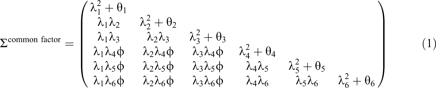
Figure 1 provides a graphical representation of a composite factor model and the corresponding common factor model. Both models consist of two related constructs with three observed indicators each. The variances of the constructs are constrained to one. For the common factor model, the implied covariance matrix is then,

Figure 1.

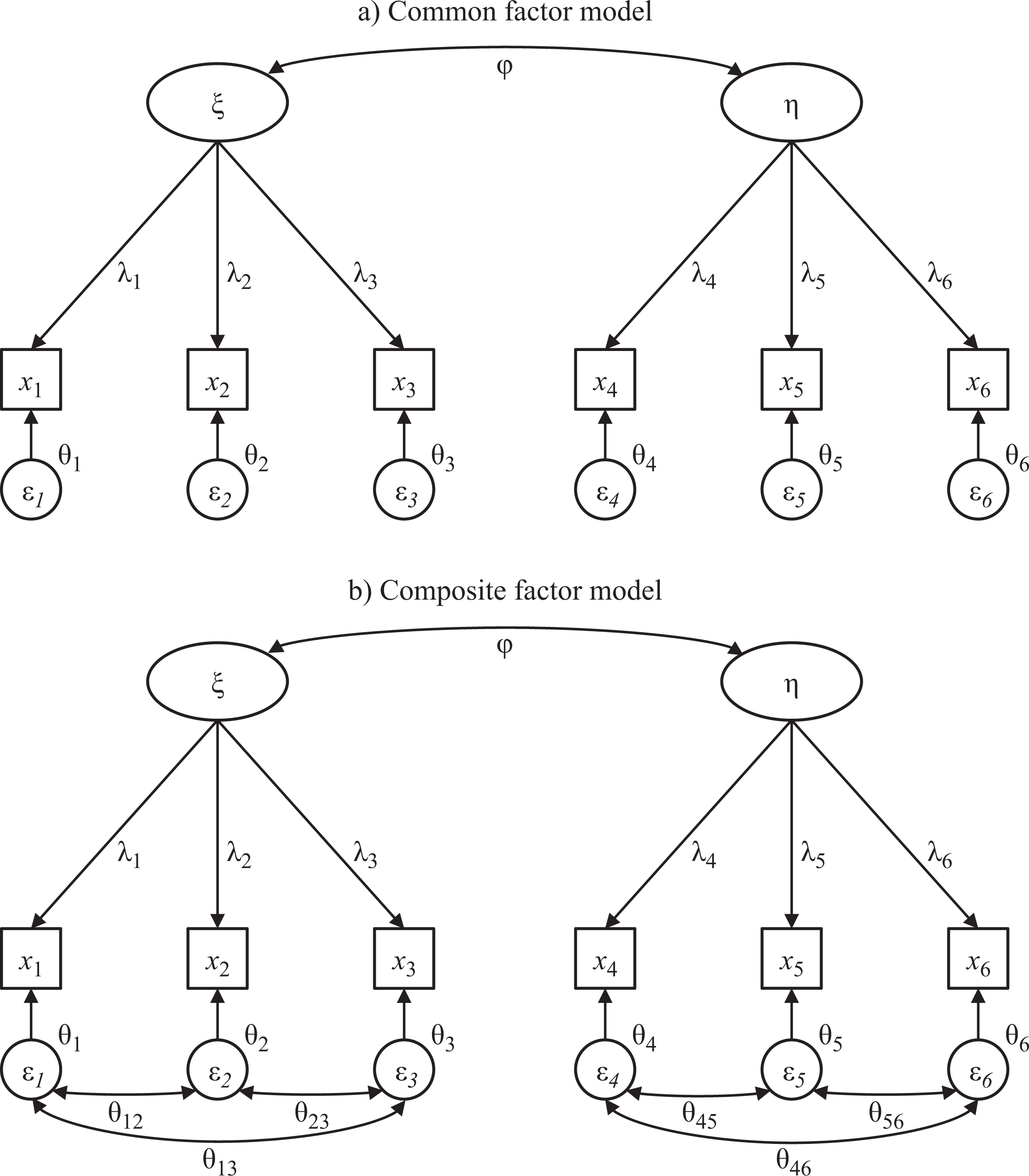
Contrasting a common factor model with a composite factor model.

${\mathrm{\Sigma }}^{\mathrm{c}\mathrm{o}\mathrm{m}\mathrm{m}\mathrm{o}\mathrm{n}\hspace{0.17em}\mathrm{f}\mathrm{a}\mathrm{c}\mathrm{t}\mathrm{o}\mathrm{r}}=\left(\begin{array}{cccccc}{\mathit{\lambda }}_1^2+{\mathit{\theta }}_1& & & & & \\ {\mathit{\lambda }}_1{\mathit{\lambda }}_2& {\mathit{\lambda }}_2^2+{\mathit{\theta }}_2& & & & \\ {\mathit{\lambda }}_1{\mathit{\lambda }}_3& {\mathit{\lambda }}_2{\mathit{\lambda }}_3& {\mathit{\lambda }}_3^2+{\mathit{\theta }}_3& & & \\ {\mathit{\lambda }}_1{\mathit{\lambda }}_4\mathit{\varphi }& {\mathit{\lambda }}_2{\mathit{\lambda }}_4\mathit{\varphi }& {\mathit{\lambda }}_3{\mathit{\lambda }}_4\mathit{\varphi }& {\mathit{\lambda }}_4^2+{\mathit{\theta }}_4& & \\ {\mathit{\lambda }}_1{\mathit{\lambda }}_5\mathit{\varphi }& {\mathit{\lambda }}_2{\mathit{\lambda }}_5\mathit{\varphi }& {\mathit{\lambda }}_3{\mathit{\lambda }}_5\mathit{\varphi }& {\mathit{\lambda }}_4{\mathit{\lambda }}_5& {\mathit{\lambda }}_5^2+{\mathit{\theta }}_5& \\ {\mathit{\lambda }}_1{\mathit{\lambda }}_6\mathit{\varphi }& {\mathit{\lambda }}_2{\mathit{\lambda }}_6\mathit{\varphi }& {\mathit{\lambda }}_3{\mathit{\lambda }}_6\mathit{\varphi }& {\mathit{\lambda }}_4{\mathit{\lambda }}_6& {\mathit{\lambda }}_5{\mathit{\lambda }}_6& {\mathit{\lambda }}_6^2+{\mathit{\theta }}_6\end{array}\right)$

1

The illustrative common factor model has 13 parameters (six loadings λ_i, six residual (error) covariances θ_i, and one structural covariance φ), which is substantially fewer than the number of moments, which is 21. The example common factor model thus has 21 – 13 = 8 degrees of freedom.

The composite factor model leaves the covariation between indicators of the same block unexplained, which means that the implied covariances between these indicators equal the empirical covariances σ_ij. This can also be expressed by additional parameters that capture the remaining indicator covariances that are not explained by their construct. Consequently, the composite factor model is less parsimonious than the common factor model. However, since the number of moments still exceeds the number of parameters (i.e., the number of degrees of freedom is greater than zero), we can refer to it as a model. ⁵

A basic principle in soft modeling is that all information between the blocks is conveyed by the composite factors (Wold, 1982). Thus, although the residual covariance matrix is no longer diagonal, it is still block diagonal. The implied covariance matrix of our example composite factor model is then,

${\mathrm{\Sigma }}^{\mathrm{c}\mathrm{o}\mathrm{m}\mathrm{p}\mathrm{o}\mathrm{s}\mathrm{i}\mathrm{t}\mathrm{e}\hspace{0.17em}\mathrm{f}\mathrm{a}\mathrm{c}\mathrm{t}\mathrm{o}\mathrm{r}}=\left(\begin{array}{cccccc}{\mathit{\sigma }}_{11}& & & & & \\ {\mathit{\sigma }}_{12}& {\mathit{\sigma }}_{22}& & & & \\ {\mathit{\sigma }}_{13}& {\mathit{\sigma }}_{23}& {\mathit{\sigma }}_{33}& & & \\ {\mathit{\lambda }}_1{\mathit{\lambda }}_4\mathit{\varphi }& {\mathit{\lambda }}_2{\mathit{\lambda }}_4\mathit{\varphi }& {\mathit{\lambda }}_3{\mathit{\lambda }}_4\mathit{\varphi }& {\mathit{\sigma }}_{44}& & \\ {\mathit{\lambda }}_1{\mathit{\lambda }}_5\mathit{\varphi }& {\mathit{\lambda }}_2{\mathit{\lambda }}_5\mathit{\varphi }& {\mathit{\lambda }}_3{\mathit{\lambda }}_5\mathit{\varphi }& {\mathit{\sigma }}_{45}& {\mathit{\sigma }}_{55}& \\ {\mathit{\lambda }}_1{\mathit{\lambda }}_6\mathit{\varphi }& {\mathit{\lambda }}_2{\mathit{\lambda }}_6\mathit{\varphi }& {\mathit{\lambda }}_3{\mathit{\lambda }}_6\mathit{\varphi }& {\mathit{\sigma }}_{46}& {\mathit{\sigma }}_{56}& {\mathit{\sigma }}_{66}\end{array}\right)=\left(\begin{array}{cccccc}{\mathit{\lambda }}_1^2+{\mathit{\theta }}_1& & & & & \\ {\mathit{\lambda }}_1{\mathit{\lambda }}_2+{\mathit{\theta }}_{12}& {\mathit{\lambda }}_2^2+{\mathit{\theta }}_2& & & & \\ {\mathit{\lambda }}_1{\mathit{\lambda }}_3+{\mathit{\theta }}_{13}& {\mathit{\lambda }}_2{\mathit{\lambda }}_3+{\mathit{\theta }}_{23}& {\mathit{\lambda }}_3^2+{\mathit{\theta }}_3& & & \\ {\mathit{\lambda }}_1{\mathit{\lambda }}_4\mathit{\varphi }& {\mathit{\lambda }}_2{\mathit{\lambda }}_4\mathit{\varphi }& {\mathit{\lambda }}_3{\mathit{\lambda }}_4\mathit{\varphi }& {\mathit{\lambda }}_4^2+{\mathit{\theta }}_4& & \\ {\mathit{\lambda }}_1{\mathit{\lambda }}_5\mathit{\varphi }& {\mathit{\lambda }}_2{\mathit{\lambda }}_5\mathit{\varphi }& {\mathit{\lambda }}_3{\mathit{\lambda }}_5\mathit{\varphi }& {\mathit{\lambda }}_4{\mathit{\lambda }}_5+{\mathit{\theta }}_{45}& {\mathit{\lambda }}_5^2+{\mathit{\theta }}_5& \\ {\mathit{\lambda }}_1{\mathit{\lambda }}_6\mathit{\varphi }& {\mathit{\lambda }}_2{\mathit{\lambda }}_6\mathit{\varphi }& {\mathit{\lambda }}_3{\mathit{\lambda }}_6\mathit{\varphi }& {\mathit{\lambda }}_4{\mathit{\lambda }}_6+{\mathit{\theta }}_{46}& {\mathit{\lambda }}_5{\mathit{\lambda }}_6+{\mathit{\theta }}_{56}& {\mathit{\lambda }}_6^2+{\mathit{\theta }}_6\end{array}\right)$

2

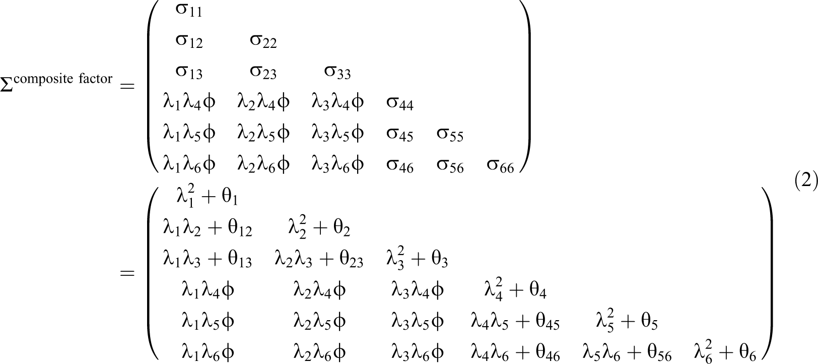
Comparing the two implied covariance matrices, it is evident that the common factor model is nested within the composite factor model because it has the same restrictions as the composite factor model plus some additional restrictions. The fact that the common factor model is nested within the composite factor model implies three possible combinations regarding model fit: (a) neither of the two models fits the data, (b) only the composite factor model fits the data, or (c) both models fit the data. This nestedness has important consequences for researchers’ choice of a model. In the first case, if neither of the two models fits the data, researchers should reject both models and refrain from interpreting estimates. In the second case, if only the composite factor model fits the data, researchers should use statistical techniques that are designed for composite factor models (e.g., PLS). In the third (less likely) case, if the common factor model fits the data, researchers should choose the common factor model and apply other appropriate estimation techniques (e.g., covariance-based SEM).

Composite factor models are likely far more prevalent than common factor models (Bentler & Huang, in press) and they are likely to have a higher overall model fit (Landis, Beal, & Tesluk, 2000). Moreover, the use of composite factor models in SEM occurs more often than one might expect. For example, the standard recipes to counter Heywood cases—fixing the error variance to zero or a small positive value—essentially abandon the common factor model for a mix between a common factor and a composite factor model (Bentler, 1976). Similarly, modifying an initial common factor model such that measurement errors are allowed to correlate coincides with a move toward a composite factor model.

Bearing the nature of the composite factor model in mind also helps better understand the nature of the alleged bias in PLS estimates. It is critical to first realize that the implied covariances between indicators of different constructs as determined by PLS are unbiased (Areskoug, 1982; Lohmöller, 1989). In other words, PLS estimates are not inherently biased, but only appear to be biased when interpreted as effects between common factors instead of effects between composite factors. Hence, bias cannot be a reason for PLS not to be seen as an SEM method. Moreover, while the lack of an overidentification test in PLS has repeatedly been criticized (e.g., Gefen et al., 2011; Hair et al., 2011), there is in fact no reason that prevents the testing of the discrepancy between the observed covariance matrix and PLS’s model-implied covariance matrix (and, indeed, we do this later when addressing Critique 3). We conclude, therefore, that PLS is clearly an SEM method that is designed to estimate composite factor models.

Critique 2: Are PLS Construct Scores More Reliable Than Sum Scores?

According to R&E, it is a myth that “PLS reduces the effect of measurement error” (p. 434). In fact, they claim that if anything, PLS provides “lower reliability composites than even simple summed scales” (p. 436). Neither statement is universally true and should therefore not be taken at face value.

While PLS does not completely eliminate the effects of measurement error, it does reduce it substantially. ⁶ This is because component methods with multiple indicators achieve a degree of adjustment for unreliability, due to the very nature of weighted composites (e.g., Creager & Valentine, 1962; Ley, 1972; Mulaik, 2010; Rigdon, 2012). Let C be a composite of p weighted variables x_i (i = 1, … p)

$C=\sum _{i=1}^p{w}_i{x}_i,$

3

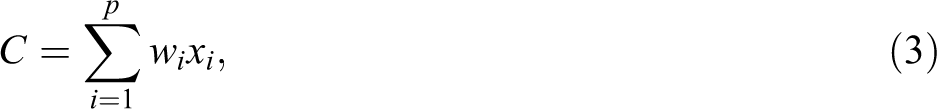
where the w_i are the weights for multiplying each respective variable before adding it to the composite. Then, the variance of the composite C is given by

${\mathit{\sigma }}_C^2=\sum _{i=1}^p{w}_i{\mathit{\sigma }}_i^2+2\sum _{i=1}^p\sum _{j=1}^{i-1}{w}_i{w}_j{\mathit{\sigma }}_{ij},$

4

where ${\mathit{\sigma }}_i^2$ is the variance of x_i and ${\mathit{\sigma }}_{ij}$ (i = 1 to p, j = 1 to i, i ≠ j) the covariance between two different indicators x_i and x_j (e.g., Mulaik, 2010). Rigdon (2012) provides a perspective on this equation when he says,

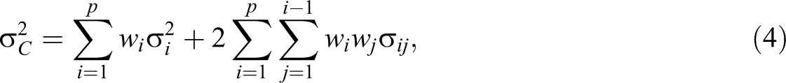
On the surface, covariances count twice. However, the variances themselves can be divided into shared variance and unshared or unique variance. The unique variance of each indicator, then, is counted only once in the variance of the composite, while shared variance is counted three times—once within the variance term of the indicator and twice among the covariances. So unique variance, including random measurement error, is substantially underweighted in forming the composite. (p. 346)

Thus, the very act of creating a weighted sum helps account for measurement error. PLS further accentuates this effect in that it places more weight on the more reliable indicators. More precisely, PLS determines the indicator weights such that the corresponding construct yields a high predictive relevance (i.e., the construct fulfills its role in the nomological net as well as possible; see Rigdon, 2012; Sarstedt, Ringle, Henseler, & Hair, in press). But if this is true then, why did R&E’s analysis yield results that contradict this logic? The answer to this question lies in their extremely limited simulation study design.

A fundamental concern in any simulation study relates to the design of the research model as well as the choice of design factors and their levels. To ensure external validity of results, the design of any simulation study needs to closely resemble setups commonly encountered in applied research (Paxton, Curran, Bollen, Kirby, & Chen, 2001). This is particularly true for simulation studies comparing the performance of statistical methods aimed at providing researchers with recommendations regarding their use in common research settings (Mooney, 1997; Rubinstein & Kroese, 2008).

Research on PLS has generated a multitude of different simulation studies that compare the technique’s performance with that of other approaches to SEM (Areskoug, 1982; Goodhue, Lewis, & Thompson, 2006, 2012; Hulland, Ryan, & Rayner, 2010; Hwang et al., 2010; Lu, Kwan, Thomas, & Cedzynski, 2011; Reinartz, Haenlein, & Henseler, 2009; Vilares, Almeida, & Coelho, 2010; Vilares & Coelho, 2013). As can be seen from Table 1, these studies vary considerably in terms of their model setup. In this context and despite the fact that most recent simulation studies use quite complex models with a multitude of constructs and path relationships, R&E chose to use a two-construct model with a single path as their basis for their simulation. ⁷ This, however, inevitably raises the question whether this model can indeed be considered representative of published research from an applied standpoint. As Paxton et al. (2001) note, when creating a model, “the Monte Carlo researcher should review structural equation model applications across a large number of journals in several areas of research to which they would like to generalize the subsequent results” (p. 291). Bearing this in mind, we revisited review studies on the use of PLS in marketing (Hair, Sarstedt, Pieper, et al., 2012), strategic management (Hair, Sarstedt, Ringle, et al., 2012), and information systems research (Ringle et al., 2012). Out of the 532 PLS models being estimated in 306 journal articles, there was exactly one model (0.2%) with two constructs by Rego (1998). More precisely, the average number of constructs was 7.94 in marketing, 7.5 in strategic management, and 8.12 in information systems, respectively. Therefore, R&E’s simulation model setup is not remotely representative of research studies using PLS.

Table 1.

Prior Simulation Studies on PLS’ Performance.

Study	Model Setup		Design Factors	Factor Levels	Factor Level Combinations	Number of Replications
	Number of Constructs	Number of Paths
Areskoug (1982)	2	1	Sample size	5	20	n/s
			Number of indicators	4
Reinartz et al. (2009)	6	9	Sample size	5	240	200
			Number of indicators	4
			Loadings	4
			Data distribution	3
Hulland et al. (2010)	6	5	Sample size	5	240	50
			Number of indicators	3
			Construct correlations	2
			Variance explained	2
			Data distribution	4
Hwang et al. (2010)	3	2	Sample size	5	20	500
			Data distribution	2
			Model specification	2
Vilares et al. (2010)	6	10	Model specification and data distribution	3	3	1,000
Lu et al. (2011)	5	4	Sample size	5	90	500
			Number of indicators	3
			Loadings	2
			Path coefficients	3
Goodhue et al. (2012) a	5	4	Study 1
			Sample size	5	5	500
	5	4	Study 2
			Sample size	2	10	500
			Data distribution	5
	5	4	Study 3
			Sample size	4	8	500
			Loadings	2
	7	9	Study 4
			Sample size	4	16	500
			Data distribution	2
			Model complexity	2
Vilares and Coelho (2013)	6	10	Sample size	6	12	1,000/1,500b
			Data distribution	2
Rönkkö and Evermann (2013)	2	1	Study 1 (Myth 2)
			Path coefficients	2	2	500
			Study 2 (Myth 3)
			Model specification	4	4	500
			Study 3 (Myth 4)
			Path coefficients	2	2	500
			Study 4 (Myth 5)
			Path coefficients	2	6	500
			Sample size	3

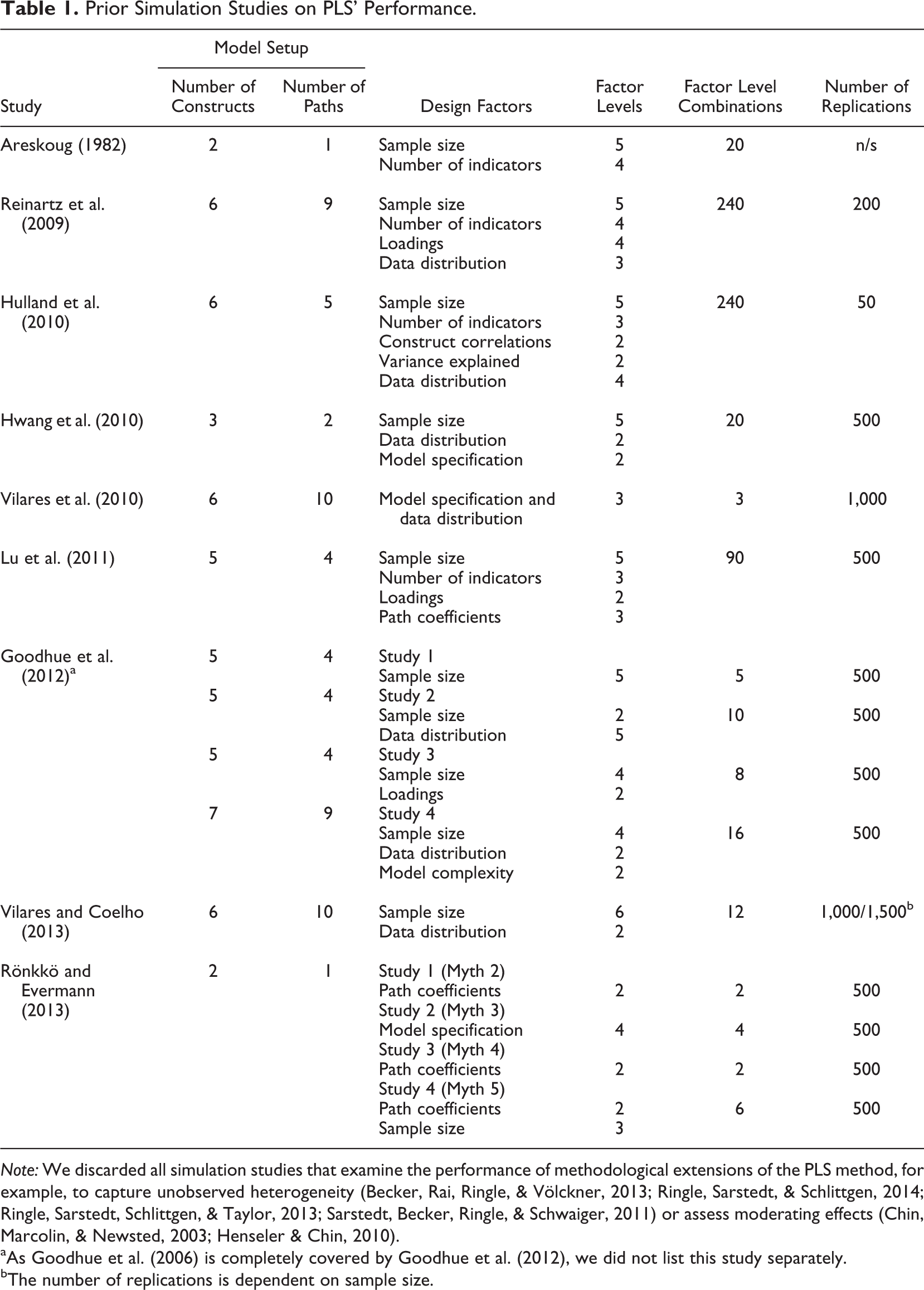
Note: We discarded all simulation studies that examine the performance of methodological extensions of the PLS method, for example, to capture unobserved heterogeneity (Becker, Rai, Ringle, & Völckner, 2013; Ringle, Sarstedt, & Schlittgen, 2014; Ringle, Sarstedt, Schlittgen, & Taylor, 2013; Sarstedt, Becker, Ringle, & Schwaiger, 2011) or assess moderating effects (Chin, Marcolin, & Newsted, 2003; Henseler & Chin, 2010).

^aAs Goodhue et al. (2006) is completely covered by Goodhue et al. (2012), we did not list this study separately.

^bThe number of replications is dependent on sample size.

In addition to the model setup, researchers need to carefully decide on the relevant factors and their levels. Comparing R&E’s simulation study with prior research in terms of design factors (see Table 1) further exposes the very limited scope of their study. Specifically, R&E vary neither the factor loadings nor the sample size, “one of the most important variables in a simulation” (Paxton et al., 2001, p. 294) and of particular relevance to PLS due to its well-known consistency at large property (e.g., Hui & Wold, 1982). The only factor that R&E vary is the standardized path coefficient between the two constructs across the two levels of 0 and 0.3, implying R ² values of 0 and 0.09. However, Paxton et al. (2001) recommend “that the R ²s take values that are representative of the areas of research with which one is most concerned. For instance, R ² values with cross-sectional, individual-level data frequently range between 0.2 and 0.8” (p. 297). This is also true for PLS research in, for example, strategic management where the average R ² in the studies reviewed by Hair, Sarstedt, Pieper, et al. (2012) was 0.36.

Against this background, we first replicate R&E’s setup by estimating a two-construct model with 100 observations, indicator loadings of 0.6, 0.7, and 0.8, and two conditions for the structural model coefficient (Condition a: β = 0; Condition b: β = 0.3). Next, we add a condition in which the standardized path coefficient has a value of 0.5, implying an R ² value more commonly encountered in applied research of .25 (Condition c). In a third step, we examine how an increased sample size of 500 observations—as routinely assumed in simulation studies in SEM in general (Paxton et al., 2001) and PLS in particular (Hulland et al., 2010; Hwang et al., 2010; Reinartz et al., 2009; Vilares & Coelho, 2013)—would influence the findings (Condition d). In a fourth step, and in line with the results of prior PLS reviews (Hair, Sarstedt, Pieper, et al., 2012; Hair, Sarstedt, Ringle, et al., 2012; Ringle et al., 2012), we consider a more heterogeneous loading pattern (0.5/0.7/0.9; Condition e). Last, to capture the typically larger complexity of models, our simulation also includes a population model with four constructs (Condition f) as shown in Figure 2. ⁸

Figure 2.

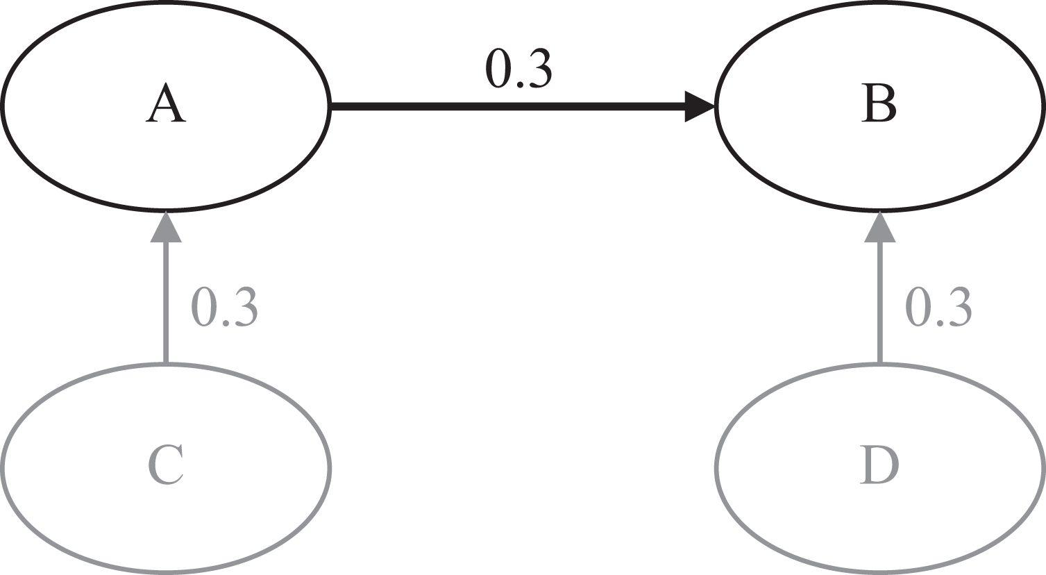
Population model with four constructs.

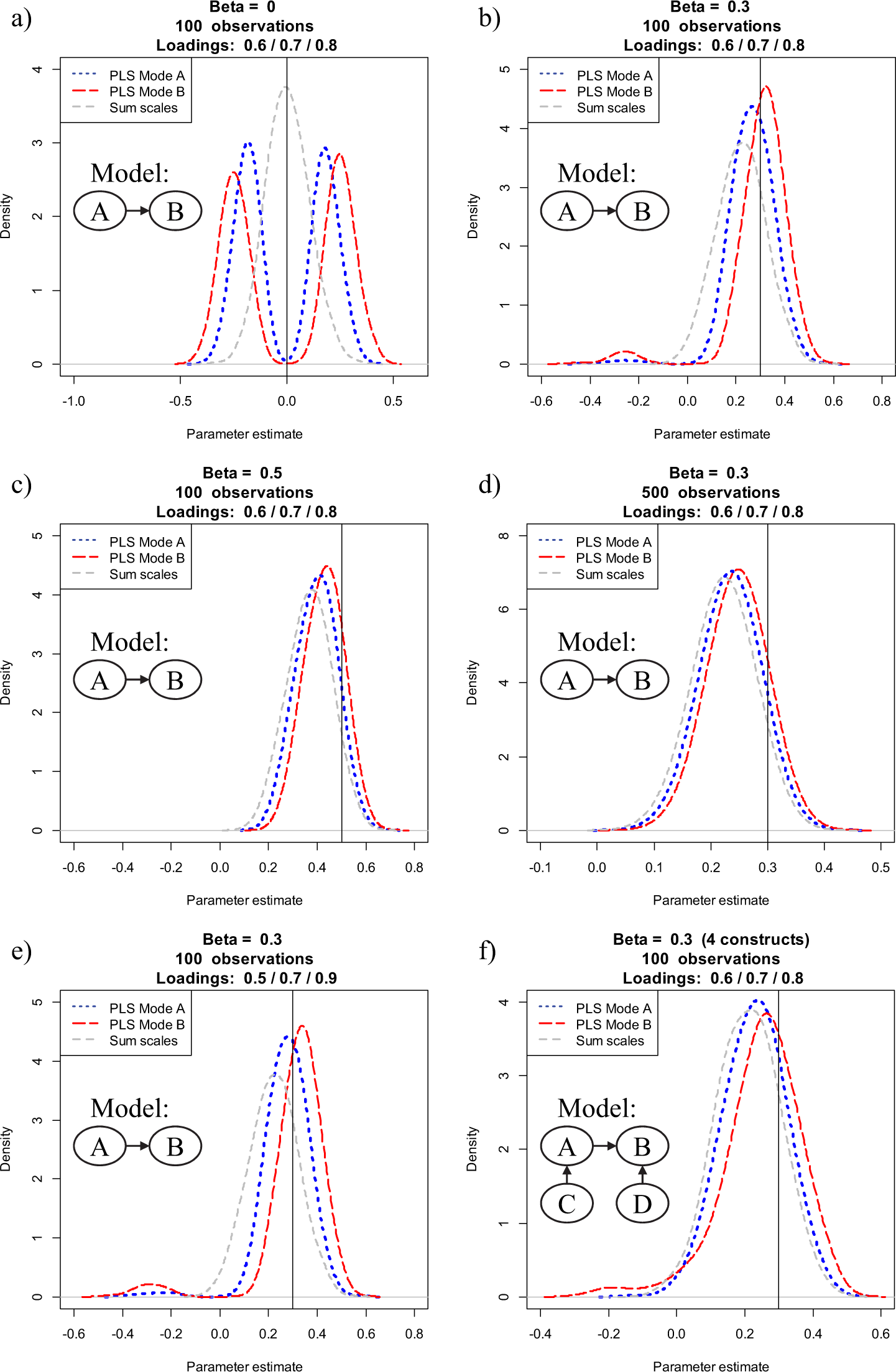
Figure 3 provides a graphical representation of the reliabilities of construct A as obtained through our Monte Carlo simulation. The results of our replication in Panels a and b are consistent with R&E’s findings. For both PLS modes, sum scores provide better (more reliable) construct scores, and PLS Mode B performs substantially worse than Mode A. However, as can also be seen in Figure 3, a different picture emerges when we vary one or more factor levels. For example, when increasing the effect size between the two constructs to a moderate (β = 0.5) level, PLS Mode A most times yields more reliable construct scores than sum scores. Likewise, although still not fully matching up with PLS Mode A or sum scores, PLS Mode B performs considerably better than when assuming no effect (β = 0) or a small effect (β = 0.3). An increase of sample size also decreases differences between the three estimation modes, with PLS Mode A outperforming sum scores. The performance of PLS Mode A relative to sum scores improves even more when assuming a more heterogeneous set of indicators. Specifically, when assuming indicator loadings of 0.5, 0.7, and 0.9, both PLS Mode A and Mode B perform considerably better than in R&E’s initial setup. This result is not surprising since—as noted earlier—PLS prioritizes indicators according to their predictive validity; that is, those indicators with a smaller error variance contribute more strongly to the measurement of the latent variables (e.g., Henseler, Ringle, & Sinkovics, 2009). Last, embedding the latent variables in a broader nomological net also improves the performance of both PLS Modes, with Mode A again outperforming sum scores (Mode B is again dominated by the other estimation techniques).

Figure 3.

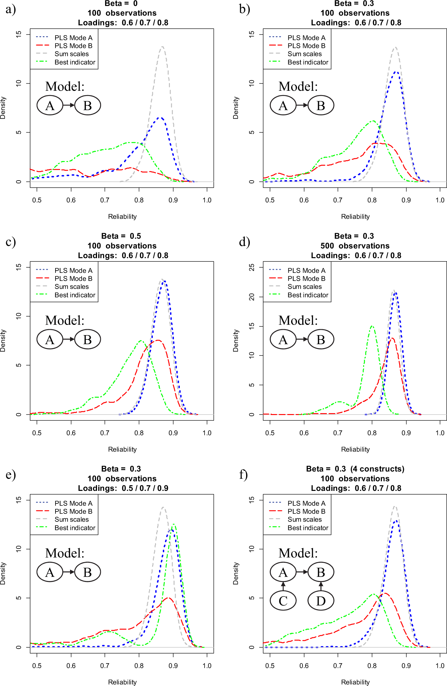
Distribution of reliability for PLS Mode A, PLS Mode B, sum scales, and the most reliable indicator over 500 replications.

Figure 3 also includes the reliability of the indicator with the highest loading. This ‘best’ indicator serves as a naïve benchmark for PLS’s capability of reducing measurement error. It is evident that construct scores obtained through PLS Mode A generally outperform the best item. Not surprisingly, the only exception is Condition e, where one indicator has a particularly high reliability (0.9).

Table 2 provides an overview of the average reliability scores of PLS Mode A, sum scores, and the best indicator estimation, and it indicates the percentage of simulation runs where PLS Mode A provided better (i.e., more reliable) construct scores. ⁹ PLS Mode A outperforms the best indicator across all model constellations, providing support for the capability of PLS to reduce measurement error. Furthermore, only in the two model constellations examined by R&E does PLS Mode A lag behind sum scores in terms of reliability. In contrast, in all other, likely much more realistic settings (e.g., Hair, Sarstedt, Pieper, et al., 2012; Hair, Sarstedt, Ringle, et al., 2012; Ringle et al., 2012), PLS Mode A clearly outperforms sum scores.

Table 2.

Simulation Results: Reliability of PLS Mode A, Sum Scales, and Best Indicator.

Condition	LVs	Loading Pattern	Beta	N	Average Reliability			PLS Mode A Outperforms …
					PLS Mode A	Sum Scores	Best Indicator	Sum Scores (%)	Best Indicator (%)
a	2	0.6/0.7/0.8	0.0	100	0.717	0.862	0.706	18.6	76.6
b	2	0.6/0.7/0.8	0.3	100	0.843	0.862	0.751	48.6	97.2
c	2	0.6/0.7/0.8	0.5	100	0.867	0.862	0.773	74.0	99.6
d	2	0.6/0.7/0.8	0.3	500	0.868	0.863	0.782	83.6	100.0
e	2	0.5/0.7/0.9	0.3	100	0.871	0.867	0.842	75.8	54.0
f	4	0.6/0.7/0.8	0.3	100	0.858	0.862	0.727	59.2	98.0

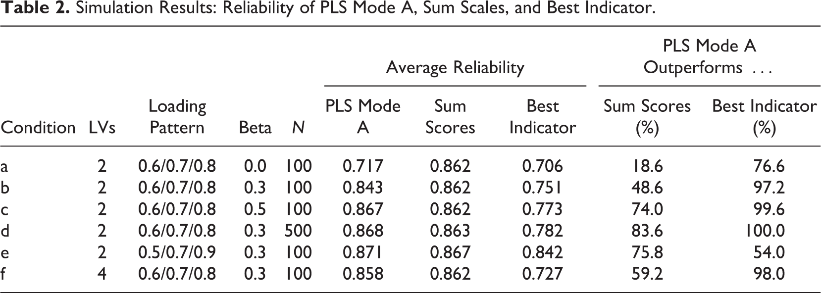
We conclude that PLS reduces measurement error but does not eliminate it. PLS should be preferred over regression on sum scores if there is sufficient information available to let PLS estimate construct weights under Mode A. Obviously, PLS construct scores can only be better than sum scores if the indicators vary in terms of the strength of relationship with their underlying construct. If they do not vary, any method that assumes equally weighted indicators will outperform PLS. We thus conclude that if the indicators differ in quality and PLS has sufficient information to estimate different weights under Mode A, the resulting PLS construct scores will be more reliable than sum scores.

Critique 3: Can PLS Be Used to Validate Measurement Models?

R&E examined to what extent selected model evaluation criteria help researchers detect measurement model misspecification. Based on a simulation study with four population models, they found that the selected evaluation criteria did not reliably distinguish between correctly specified and misspecified models. R&E thus concluded that “the idea that PLS results can be used to validate a measurement model is a myth” (p. 438).

Again, the conclusion reached by R&E must be viewed with great skepticism. Not only did they mistakenly assume that PLS estimates a common factor model rather than a composite factor model, they also committed several calculation and reporting errors and claimed—without any supporting empirical evidence—that covariance-based SEM would have a better performance in detecting model misspecification than PLS. More specifically, R&E mixed up two models in their reporting (the values for Model 2 were reported under Model 3 in their Table 4 and vice versa). They also calculated four out of five statistics incorrectly. First, they calculated both the composite reliability as well as the average variance extracted (AVE) assuming that the second population model (with only one construct) was estimated. Instead, R&E should have calculated values for each of the two constructs—further analysis typically ensuring that the minimum of the two AVE values is above 0.5. As a result, this Fornell–Larcker criterion is also miscalculated since it builds on the AVE statistic. Moreover, R&E did not compute the standardized root mean square residual (SRMR) as the root mean square discrepancy between the observed correlations and the model-implied correlations (Hu & Bentler, 1998, 1999), but the root mean square residual covariance (RMS_theta) as suggested by Lohmöller (1989, Equation 2.118). Put simply, the vast majority of the reported values in R&E’s Table 4 are simply wrong. Finally, R&E did not assess the exact model fit of the PLS path model, so it remains unclear whether the PLS estimates can truly be used for model testing.

To verify and where necessary to correct R&E’s findings, we replicated their simulation study. Figure 4 shows the four population models used by R&E. For each population model, we generated 500 data sets with 100 observations each, and estimated the parameters using the first model, no matter by which population model the data were created. ¹⁰ Analogous to R&E, we examine Jöreskog’s rho (as a measure of composite reliability), the AVE, and the Fornell–Larcker criterion (Fornell & Bookstein, 1982; Fornell & Larcker, 1981) as well as the relative GoF (GoF_rel; Esposito Vinzi, Trinchera, & Amato, 2010) and the RMS_theta (Lohmöller, 1989). Since R&E apparently intended to examine the SRMR, but actually did not, we also include this statistic in our analysis. We determine the SRMR for PLS in congruence with the model that is actually estimated, that is, an SRMR for a composite factor model. ¹¹ The model-implied covariance-matrix of the PLS path model is computed using Equation 2, and we determine the exact fit of the composite factor model by means of bootstrapping the conventional likelihood function. In essence, this constitutes a confirmatory composite analysis. Finally, to facilitate a comparison between PLS and covariance-based SEM, we also report the exact fit and the SRMR as obtained from covariance-based SEM. Table 3 reports the results of R&E and contrasts them with our own findings.

Figure 4.

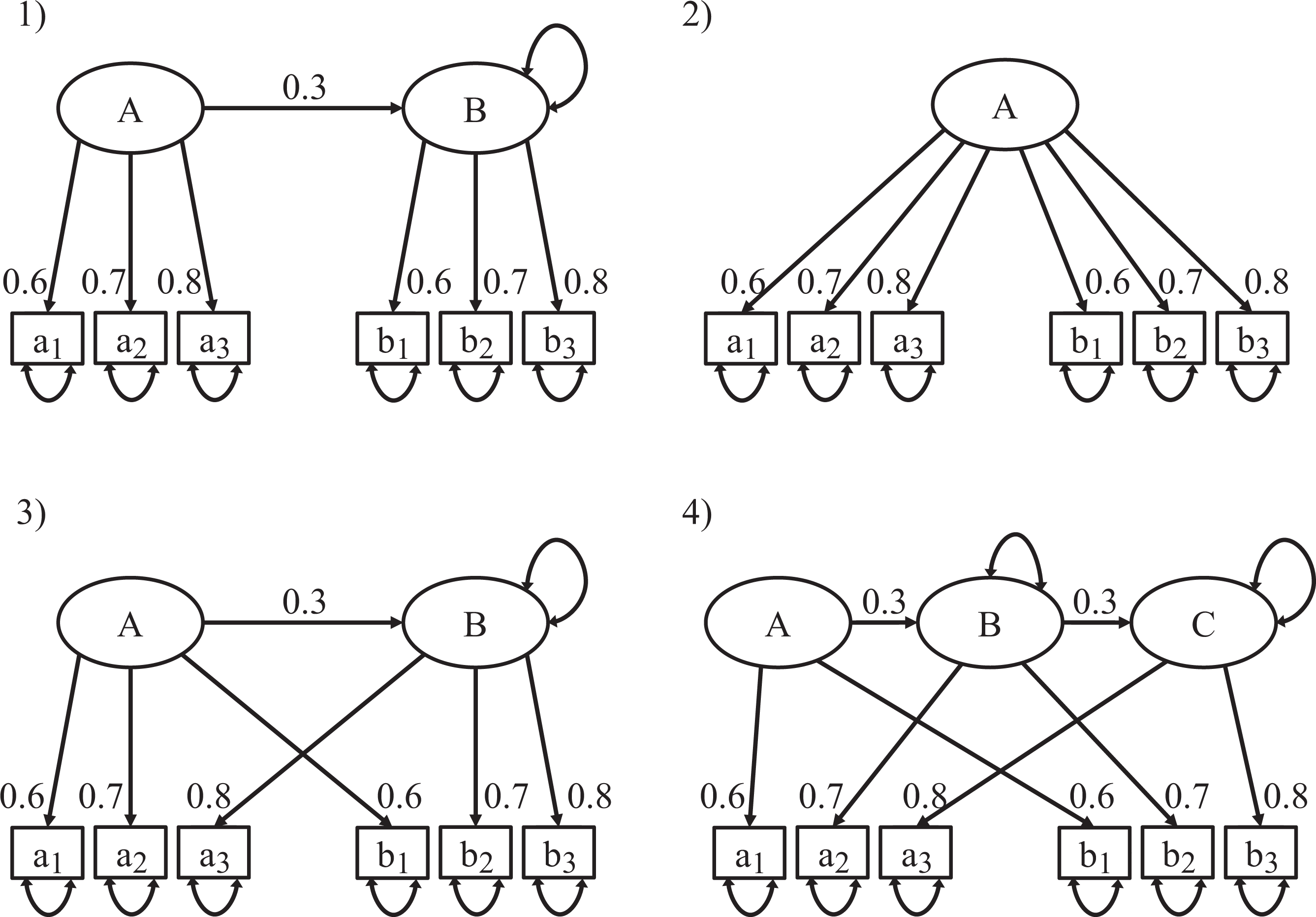
The four population models used by R&E.

Table 3.

Simulation Results: Performance of Different Indices of PLS and Covariance-Based SEM (CB-SEM) for Measurement Model Validation.

Model	Statistic	R&E				Our Replication
		5%	Mdn	95%	Accept? (%)	5%	Mdn	95%	Accept? (%)
1)	PLS: Jöreskog’s rho	0.875	0.940	0.960	98.0	0.769	0.844	0.881	97.4
	PLS: AVE	0.563	0.646	0.695	98.2	0.544	0.645	0.713	97.0
	PLS: Fornell–Larcker	0.454	0.563	0.631	100.0	0.438	0.563	0.645	100.0
	PLS: relative GoF	0.620	0.859	0.971	28.6	0.615	0.857	0.968	35.8
	PLS: RMStheta	0.076	0.090	0.112	13.6	0.076	0.091	0.113	—
	PLS: exact fit	Values only for the 482 simulation runs (96.4%) in which CB-SEM converged.				—	—	—	95.6
	PLS: SRMR					0.022	0.039	0.061	100.0
	CB-SEM: exact fit (p)					0.049	0.469	0.949	94.8
	CB-SEM: SRMR					0.025	0.045	0.071	98.5
2)	PLS: Jöreskog’s rho	0.917	0.947	0.965	100.0	0.809	0.853	0.884	100.0
	PLS: AVE	0.596	0.658	0.710	100.0	0.587	0.660	0.718	100.0
	PLS: Fornell–Larcker	−0.012	0.075	0.165	92.2	−0.025	0.074	0.166	91.2
	PLS: relative GoF	0.955	0.979	0.993	100.0	0.956	0.981	0.994	100.0
	PLS: RMStheta	0.080	0.093	0.110	4.2	0.080	0.093	0.107	—
	PLS: exact fit	Values only for the 443 simulation runs (88.6%) in which CB-SEM converged.				—	—	—	95.6
	PLS: SRMR					0.025	0.039	0.054	100.0
	CB-SEM: exact fit (p)					0.040	0.443	0.937	93.2
	CB-SEM: SRMR					0.018	0.032	0.047	100.0
3)	PLS: Jöreskog’s rho	0.711	0.844	0.895	95.4	0.654	0.729	0.778	77.0
	PLS: AVE	0.426	0.497	0.557	48.0	0.405	0.481	0.542	33.0
	PLS: Fornell–Larcker	−0.025	0.075	0.193	89.2	−0.043	0.062	0.169	80.8
	PLS: relative GoF	0.882	0.934	0.971	88.0	0.894	0.945	0.972	94.0
	PLS: RMStheta	0.148	0.179	0.211	0.0	0.149	0.176	0.212	—
	PLS: exact fit	Values only for the 432 simulation runs (86.4%) in which CB-SEM converged.				—	—	—	1.2
	PLS: SRMR					0.083	0.116	0.148	3.0
	CB-SEM: exact fit (p)					0.000	0.000	0.000	0.0
	CB-SEM: SRMR					0.108	0.149	0.192	0.0
4)	PLS: Jöreskog’s rho	0.542	0.783	0.861	82.4	0.408	0.639	0.716	11.2
	PLS: AVE	0.392	0.452	0.517	11.2	0.348	0.406	0.470	1.2
	PLS: Fornell–Larcker	−0.265	−0.175	−0.081	0.2	−0.148	−0.041	−0.082	29.4
	PLS: relative GoF	0.904	0.958	0.991	94.8	0.901	0.960	0.991	95.2
	PLS: RMStheta	0.184	0.213	0.244	0.0	0.145	0.175	0.206	—
	PLS: exact fit	Values only for the 416 simulation runs (83.2%) in which CB-SEM converged.				—	—	—	0.0
	PLS: SRMR					0.088	0.115	0.143	1.2
	CB-SEM: exact fit (p)					0.000	0.000	0.000	0.0
	CB-SEM: SRMR					0.093	0.125	0.158	0.2

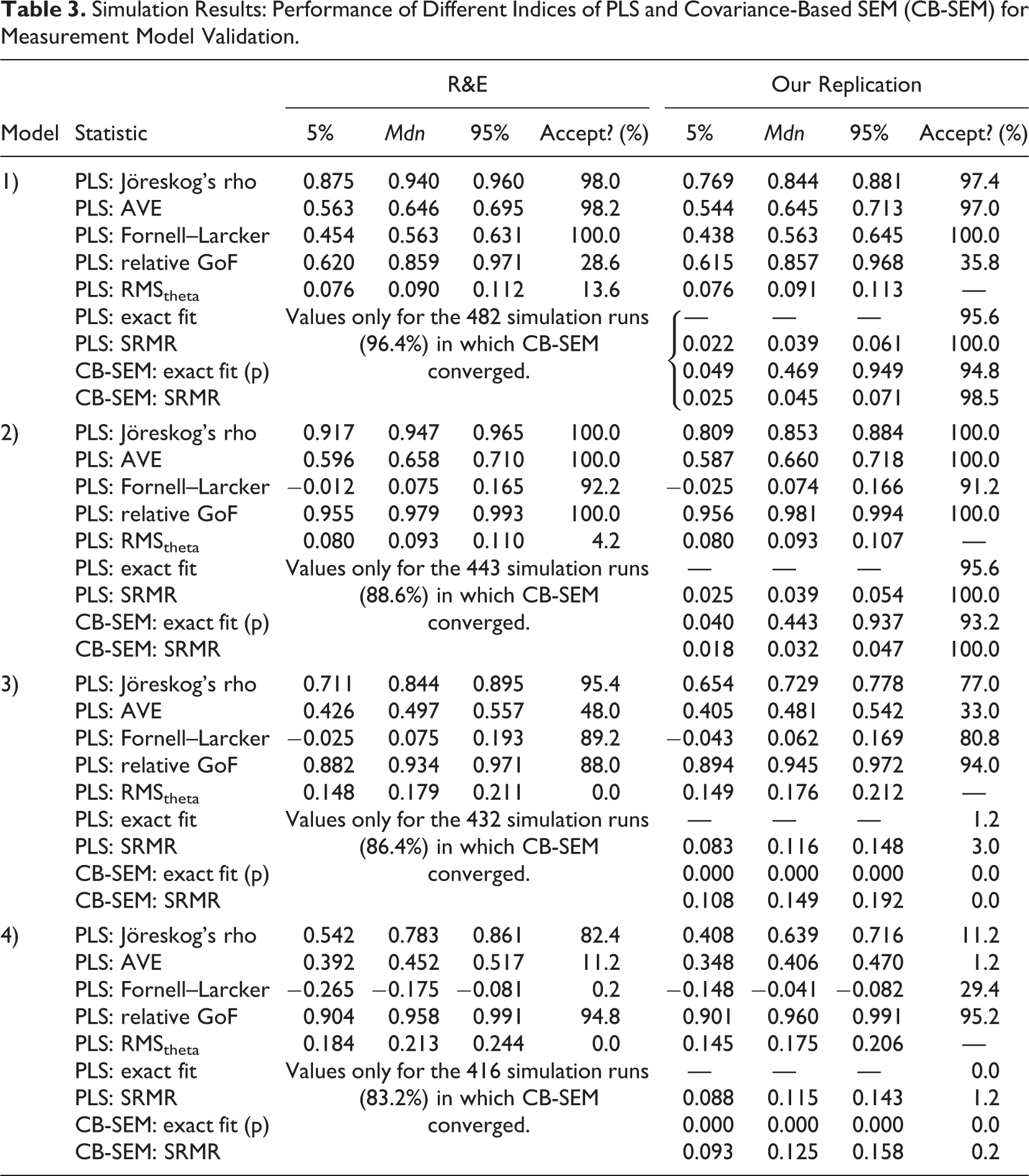
Model 1 represents a case in which the estimated model is isomorphic to the population model. Optimally, all assessment criteria should indicate that the model is acceptable. We find that this is the case for all assessment criteria other than the relative GoF and RMS_theta. With an acceptance rate of 35.8%, the relative GoF is not really able to recognize that the estimated model is acceptable. This finding is consistent with Henseler and Sarstedt (2013), who likewise report that the family of GoF indices is not suitable for model comparisons and for detecting model misspecification. In fact, numerous articles clearly advise against the use of the GoF indices to validate PLS path models globally (Hair, Hult, Ringle, & Sarstedt, 2014; Hair, Ringle, & Sarstedt, 2013; Hair, Sarstedt, Pieper, et al., 2012; Hair, Sarstedt, Ringle, et al., 2012), which makes R&E’s inclusion of this statistic highly questionable. ¹² The only other criterion, which (erroneously) rejected Model 1 in R&E’s study, is RMS_theta (which, as noted, R&E mistakenly labeled as SRMR). However, the threshold used for SRMR cannot be readily transferred to RMS_theta. Lohmöller (1989) suggests only that the outer model is satisfactory “if the residual covariances between blocks are near zero” (p. 55).

Model 2 represents a situation in which an overparameterized model is estimated. Instead of assuming (and thus constraining) a correlation of one between the two constructs, the interconstruct correlation is freely estimated. In accordance with R&E, we find that none of the assessment criteria recommended for use in combination with PLS detect this lack of discriminant validity. This is particularly surprising with regard to the Fornell–Larcker criterion (Fornell & Larcker, 1981), which is intended exactly for conditions like the present one. However, we further note that the SRMRs of both PLS and covariance-based SEM as well as the relevant exact tests of fit likewise do not detect that the model is misspecified. While the acceptance rate of covariance-based SEM is somewhat lower than that of PLS (93.2% vs. 95.6%), it is obvious that neither PLS nor covariance-based SEM can reliably detect this form of misspecification.

Model 3 represents a situation in which two indicators are assigned to the wrong construct. While the AVE actually performs somewhat better than initially reported by R&E, the conventional assessment criteria of PLS do not reliably detect the misspecification. In contrast, the exact fit test and the SRMR of the composite factor model perform substantially better with acceptance rates of 1.4% and 3.0%, respectively. While, at first, the acceptance rate of PLS appears considerably worse than that of covariance-based SEM, the large number of Heywood cases—negative variances occur in more than 60% of the simulation runs—puts this into perspective. Ultimately, our overall evidence indicates that PLS provides a more reliable indication of model misspecification than covariance-based SEM.

Model 4 represents a situation in which the indicators are actually evoked by three constructs instead of two. Under this condition, the conventional PLS assessment criteria exhibit a better performance than previously. In particular, the AVE detects this form of misspecification reliably. Moreover, composite reliability performs relatively well. Again, the most reliable indicators of model misspecification are the exact fit and the SRMR. In particular, the test of exact fit rejects Model 4 in all cases. As in Model 3, the high number of Heywood cases (up to 100%, depending on the software implementation) renders the use of covariance-based SEM impracticable and puts its acceptance rate into perspective.

We conclude that while R&E’s critique on the efficacy of conventional measurement model assessment criteria (composite reliability, AVE, and the Fornell–Larcker criterion) is justified, their central conclusion is not. Researchers can rely on PLS-based assessment criteria such as the test of exact fit (i.e., statistical inference on the discrepancy between the empirical covariance matrix and the covariance matrix implied by the composite factor model) or the SRMR to determine to what extent the composite factor model fits the data. An additional criterion may be the RMS_theta, which, in our study, was substantially higher for misspecified models than for correct models. Future research should try to identify an optimal threshold value for RMS_theta to give researcher an additional instrument to recognize misspecified PLS path models. ¹³ We conclude that PLS can help detect a wide spectrum of measurement model misspecifications as long as a composite factor model is assumed and the test of exact fit and/or the SRMR are used for model validation purposes.

Critique 4: Can PLS Be Used for Null Hypothesis Significance Testing (NHST) of Path Coefficients?

Based on a simulation study, R&E conclude that, because the distribution of parameter estimates is not normal but bimodal in shape when no effect between the two constructs under consideration is assumed (i.e., β = 0), PLS cannot be used in null hypothesis significance testing (NHST). Furthermore, they recommend that “bootstrapped confidence intervals of PLS estimates should not be used for making statistical inferences until further research is available to show under which conditions, if any, the bootstrapped distribution follows the sampling distribution of the PLS parameter estimate” (p. 440). Considering that PLS is routinely used for testing relationships derived from formal hypotheses (Rigdon, 2013) and that prior simulation studies have underlined PLS’s suitability for hypothesis testing across a wide range of model setups (e.g., Reinartz et al., 2009), the claim that PLS cannot be used in NHST is certainly disturbing. But is it true?

R&E’s claim is based on two arguments, namely that (a) the distribution of parameter estimates is not normal but bimodal in shape and (b) the difference between the distribution of parameter estimates and the empirical bootstrap distribution renders NHST impossible. Both arguments stand on quicksand. Regarding (a), R&E only considered one population model, but generalize to all models with path coefficients of zero. It remains thus to be seen whether the problem of bimodal distributions applies to all path coefficients of zero. Regarding (b), R&E’s argument is even shakier because they did not empirically investigate the robustness of NHST with respect to differences in distribution.

To shed further light on these issues, we replicate and extend R&E’s simulation design in a manner analogous to that for Critique 2 earlier. We first examine whether the bimodal shape of the parameter estimate distribution holds for other settings. What did we find? While our results shown in Figure 5 parallel those of R&E for a two-construct model with 100 observations, indicator loadings of 0.6, 0.7, and 0.8, and two conditions for the structural model coefficients (β = 0 and β = 0.3), this is not the case when the simulation design is varied slightly. More precisely, when increasing the standardized path coefficient to a moderate level (β = 0.5) or increasing the sample size (N = 500) or embedding the latent variables in a nomological net with constant effects (see Figure 2), parameter estimates clearly follow a unimodal distribution. Not surprisingly, assuming more heterogeneous loadings does not influence the shape of the distribution, which is in line with Reinartz et al.’s (2009) findings. In addition, the results show that the parameter bias is consistently smaller in PLS Mode A and Mode B estimation as compared to sum scores, making PLS more appealing from an accuracy perspective.

Figure 5.

Distribution of parameter estimates for PLS Mode A, PLS Mode B, and sum scales over 500 replications.

Next, since R&E question the suitability of PLS for NHST without actually examining its behavior, we analyze the Type I and Type II errors that PLS produces for R&E’s population model. We use the boot package (Canty & Ripley, 2013; Davison & Hinkley, 1997) to compare four ways of determining bootstrap confidence intervals (DiCiccio & Efron, 1996): (a) normal confidence intervals, which use bootstrap estimates of standard errors and quantiles of the normal distribution; (b) percentile confidence intervals, which rely on the percentiles of the empirical bootstrap distribution to determine confidence intervals around the parameters of interest; (c) bias-corrected and accelerated confidence intervals (BCa), which employ improved percentile intervals; and (d) basic bootstrap confidence intervals, as directly derived from the bootstrap percentiles. For a more detailed description, see Davison and Hinkley (1997).

In accordance with our earlier simulation design, we vary the path coefficient, sample size, and model complexity. Table 4 shows the results of our analysis, which draws on 500 replications. Three ways of determining bootstrap confidence intervals (normal, percentile, and BCa) largely maintain the prespecified alpha protection level of 5%, whereas the basic confidence interval produces an undue number of Type I errors. With regard to Type II errors, the BCa confidence intervals turn out to show the lowest power. However, BCa confidence intervals are the only ones that under all conditions maintained the alpha protection level of 5%. Overall, the normal, the percentile, and the BCa bootstrap confidence intervals appear suitable for NHST. Among them, the percentile bootstrap confidence interval is a good compromise (Hayes & Scharkow, 2013). These results are completely in line with those of Goodhue et al. (2012), who also did not find any problematic behavior of PLS in combination with bootstrapping.

Table 4.

Simulation Results for Different Bootstrap Confidence Interval Types.

Beta	LVs	Loading Pattern	N		Bootstrapping
				Percentile (%)	BCa (%)	Normal (%)	Basic (%)
0.0	2	0.6/0.7/0.8	100	5.0	0.8	5.8	40.2
0.0	2	0.6/0.7/0.8	500	4.2	1.8	3.6	30.4
0.0	2	0.5/0.7/0.9	100	5.6	0.2	4.2	42.6
0.0	4	0.6/0.7/0.8	100	5.6	2.0	6.8	11.0
0.3	2	0.6/0.7/0.8	100	58.0	26.0	57.4	79.0
0.3	2	0.6/0.7/0.8	500	99.8	97.8	99.8	100.0
0.3	2	0.5/0.7/0.9	100	60.8	30.8	60.6	85.2
0.3	4	0.6/0.7/0.8	100	60.6	45.0	60.8	68.8

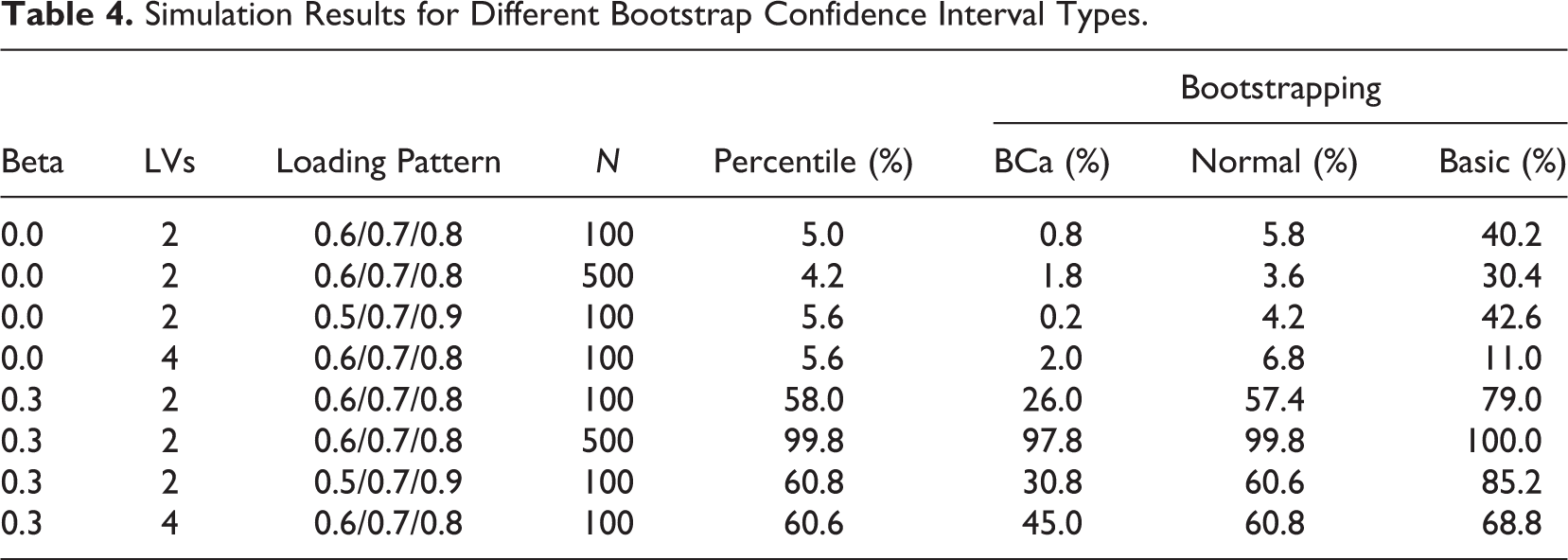
We conclude that PLS is generally suitable for NHST, even if the interrelated constructs are not embedded in a wider nomological net, if sample size is relatively low, and if expected effects are small. Researchers need to take care only that they use normal, percentile, or BCa bootstrapping, but not basic bootstrapping. Given that the dominant PLS software implementations of SmartPLS (Ringle, Wende, & Will, 2005) and PLS-Graph (Chin & Frye, 2003) already use normal bootstrapping (Temme, Kreis, & Hildebrandt, 2010), it is unlikely that researchers using this software have faced or will face problems with NHST.

Critique 5: Does PLS Have Minimal Requirements on Sample Size?

The most prominent argument for choosing PLS-SEM in many disciplines such as marketing (Hair, Sarstedt, Ringle, et al., 2012), management information systems (Ringle et al., 2012) and strategic management (Hair, Sarstedt, Pieper, et al., 2012) is the use of small sample sizes. This topic has been passionately debated in recent years (e.g., Marcoulides & Saunders, 2006) and has been empirically examined in various simulation studies (e.g., Areskoug, 1982; Goodhue et al., 2012; Hulland et al., 2010; Lu et al., 2011; Reinartz et al., 2009; Vilares & Coelho, 2013). As also emphasized in previous studies (e.g., Hair et al., 2013; Hair, Sarstedt, Pieper, et al., 2012; Hair, Sarstedt, Ringle, et al., 2012), we agree with R&E’s criticism that many authors seem to believe that sample size considerations do not play a role in the application of PLS by scholars.

Where does this idea come from then? We believe that this idea is fostered by the often cited “10 times” rule (Barclay, Higgins, & Thompson, 1995), according to which the sample size should be equal to the larger of (a) 10 times the index with the largest number of formative indicators or (b) 10 times the largest number of structural paths directed at a particular latent variable in the structural model. The argument becomes clearer if one notes that the role of sample size for SEM is twofold. On one hand, sample size is a major determinant of statistical power and therefore influences the quality of inference statistics obtained from a statistical technique (Paxton et al., 2001). On the other hand, each technique requires a certain sample size to be able to provide estimates (Hair, Anderson, Tatham, & Black, 1998). We examine both roles of sample size for SEM.

With regard to statistical power, it can be expected that covariance-based SEM, as a full-information estimator, will most of the time deliver smaller standard errors than limited-information estimators such as PLS. Empirical evidence based on simulation studies confirms this notion (Goodhue et al., 2012). Findings to the contrary—such as those by Lu et al. (2011) or Reinartz et al. (2009)—can be traced back to the differences we note above between the common factor model and the composite factor model. There are situations (population covariance matrices) in which there are effects between composite factors but not between common factors and vice versa. Depending on the population model, researchers can get the erroneous impression that one method has a higher statistical power to detect a certain effect than the other, whereas in fact the effects need to be interpreted differently (Rai, Goodhue, Henseler, & Thompson, 2013).

However, sample size not only plays a role with regard to statistical power. As Reinartz et al. (2009) show, PLS demonstrates better convergence behavior in the case of small sample sizes than covariance-based SEM. Our simulations confirm this finding. For instance, the sem package (Fox, Nie, & Byrnes, 2013) produced inadmissible solutions for all the 500 data sets drawn from the population 3 of Figure 4 (nonconvergence: 13.4%; Heywood cases: 86.4%). To verify that this poor behavior is attributable to the method itself and not a particular implementation of it, we triangulated this finding using the lavaan package version 0.5-14 (Rosseel, 2012), which produced inadmissible solutions in 63.4% of all cases (nonconvergence: 12.6%; Heywood cases: 50.8%) and Mplus version 4.21 (Muthén & Muthén, 2006), which resulted in inadmissible solutions in 70.0% of the cases (nonconvergence: 8.0%; Heywood cases: 62.0%). In contrast to covariance-based SEM, PLS always converged and always produced admissible solutions. These results are in accordance with extant research, which has found that nonconvergence and Heywood cases occur quite frequently with common factor models (Krijnen, Dijkstra, & Gill, 1998) and that PLS in general only rarely has convergence problems (Henseler, 2010).

Moreover, in contrast to covariance-based SEM, PLS can even be used if the number of observations is smaller than the number of variables (whether manifest or latent) or the number of parameters in the model. We therefore conclude that PLS can be applied in many instances of small samples when other methods fail.

Critique 6: Is PLS Appropriate for Exploratory or Early Stage Research?

R&E argue that “using PLS as an exploratory or early-stage theory testing tool does not feature strongly in the early PLS articles” (p. 442) and that only recent literature such as Hair et al. (2011) conveys this notion. This description openly misrepresents research reality. In fact, Herman Wold, the inventor of PLS, emphasized exploratory nature of PLS from the very beginning of its development:

PLS is primarily intended for research contexts that are simultaneously data-rich and theory-skeletal. The model building is then an evolutionary process, a dialog between the investigator and the computer. In the process, the model extracts fresh knowledge from the data, thereby putting flesh on the theoretical bones. At each step PLS rests content with consistency of the unknowns. As the model develops, it may be appropriate to try ML estimation with its higher aspiration of optimal accuracy. (Lohmöller & Wold, 1980, p. 1)

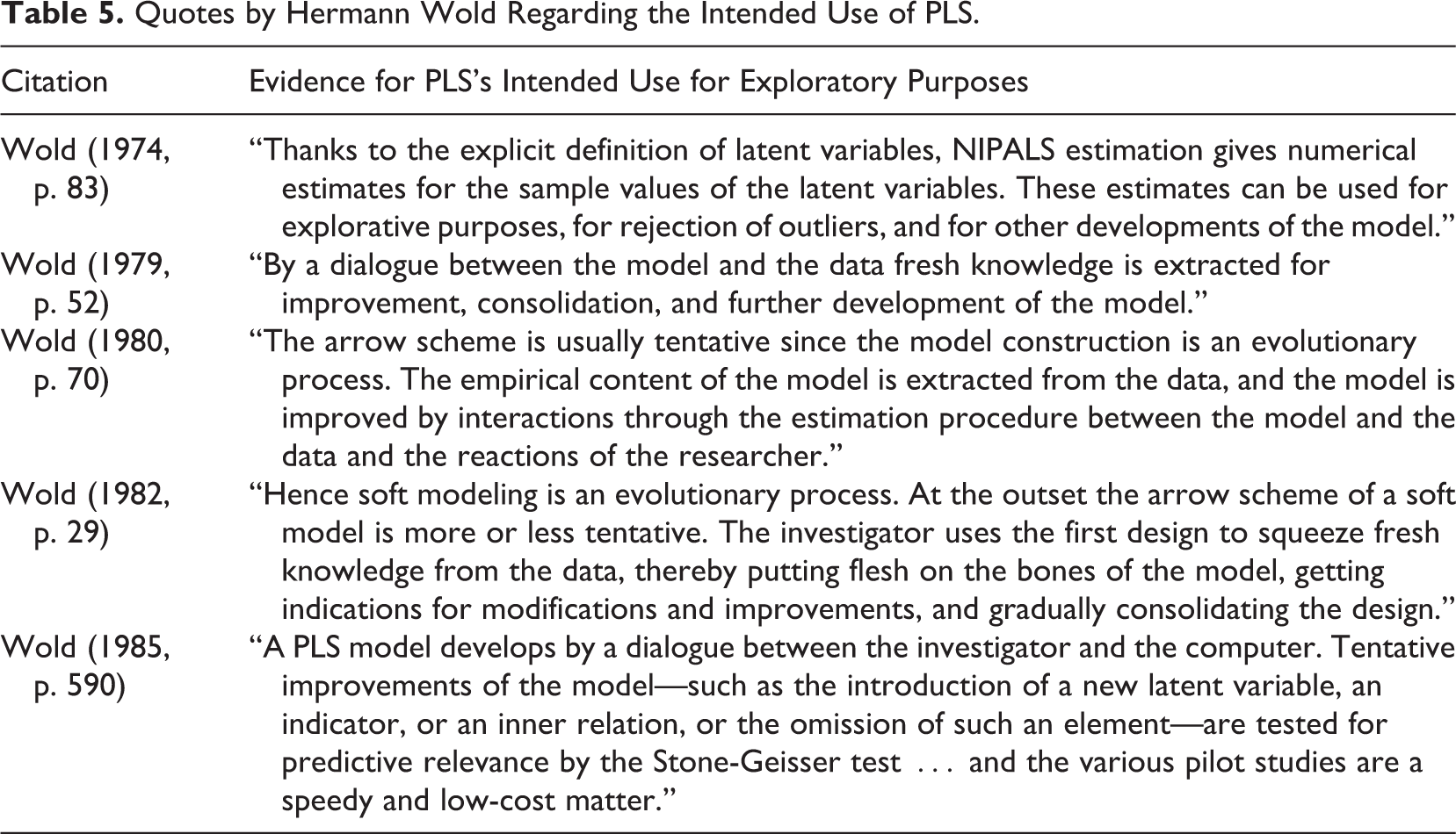
Moreover, as Table 5 clearly illustrates, Wold stressed this discovery-oriented process throughout the development phases of PLS (e.g., Wold, 1974, 1979, 1980, 1982, 1985). Rather than commit a priori to a specific model, he imagined a researcher estimating numerous models in the course of learning something about the data and about the phenomena underlying the data (Rigdon, 2013). Thus, PLS’s exploratory nature is certainly no “urban legend” but one of the driving forces of Wold’s PLS development. ¹⁴

Table 5.

Quotes by Hermann Wold Regarding the Intended Use of PLS.

Citation	Evidence for PLS’s Intended Use for Exploratory Purposes
Wold (1974, p. 83)	“Thanks to the explicit definition of latent variables, NIPALS estimation gives numerical estimates for the sample values of the latent variables. These estimates can be used for explorative purposes, for rejection of outliers, and for other developments of the model.”
Wold (1979, p. 52)	“By a dialogue between the model and the data fresh knowledge is extracted for improvement, consolidation, and further development of the model.”
Wold (1980, p. 70)	“The arrow scheme is usually tentative since the model construction is an evolutionary process. The empirical content of the model is extracted from the data, and the model is improved by interactions through the estimation procedure between the model and the data and the reactions of the researcher.”
Wold (1982, p. 29)	“Hence soft modeling is an evolutionary process. At the outset the arrow scheme of a soft model is more or less tentative. The investigator uses the first design to squeeze fresh knowledge from the data, thereby putting flesh on the bones of the model, getting indications for modifications and improvements, and gradually consolidating the design.”
Wold (1985, p. 590)	“A PLS model develops by a dialogue between the investigator and the computer. Tentative improvements of the model—such as the introduction of a new latent variable, an indicator, or an inner relation, or the omission of such an element—are tested for predictive relevance by the Stone-Geisser test … and the various pilot studies are a speedy and low-cost matter.”

While the originators of the PLS method stressed its exploratory character, this is usually not the case with applied researchers. Literature reviews show that only 43 of 306 articles (14.05%) published in marketing, strategic management, and information systems literatures mentioned “exploration” as a rationale for using PLS (Hair, Sarstedt, Pieper, et al., 2012; Hair, Sarstedt, Ringle, et al., 2012; Ringle et al., 2012). This is not all that surprising in light of the academic bias in favor of findings presented in confirmatory terms (Greenwald, Pratkanis, Leippe, & Baumgardner, 1986; Rigdon, 2013). In fact, this observation also holds for covariance-based SEM, which is traditionally viewed as a confirmatory tool. However, its actual use is far from it as researchers routinely engage in specification searches when the initially hypothesized model exhibits inadequate fit. Interestingly, this is more often the rule than the exception (e.g., Cliff, 1983; Sarstedt et al., in press). But does PLS have the necessary requisites for exploratory modeling? Contradicting the view of the originators of PLS, R&E argue that it does not, primarily because PLS cannot be used to validate models. R&E state that whereas covariance-based SEM can detect both overparameterization (by assessing the significance of path coefficients) and underparameterization (using modification indices), PLS can detect only overparameterization. Based on this observation, they conclude that PLS is not suitable for exploratory purposes. We do not agree with this conclusion for three reasons. First, R&E neglect an obvious modeling option: starting the exploratory analysis with a likely overparameterized or even saturated model and dropping nonsignificant paths. Second, as our answer to Critique 3 demonstrated, PLS can certainly be used to validate models, and at least two overall model criteria can detect underparameterization: (a) exact fit and (b) SRMR. Third, R&E fail to empirically demonstrate that covariance-based SEM performs better than PLS in finding the true model. Given the mediocre-to-poor performance of covariance-based SEM specification searches (e.g., Heene, Hilbert, Freudenthaler, & Bühner, 2012; Homburg & Dobratz, 1992), a blind faith in covariance-based SEM’s exploratory capabilities appears both unwise and unjustified.

R&E’s failure to clearly distinguish between the common factor model and the composite factor model also has consequences for their conclusions with respect to PLS’s adequacy for exploratory research. Owing to their blind adherence to the common factor model, R&E misinterpret Lohmöller: “The corollary assumed by Lohmöller, neither logically implied nor correct, is that PLS is appropriate when the researcher is not sure that the model is correct. Lohmöller [implies] that the term explorative refers to situations where the model may be incorrect” (p. 442). If things were really this way, R&E would be justified because model misspecification cannot be corrected by choosing one estimation technique over another (Henseler, 2012). Unfortunately, R&E ignore the fact that Lohmöller refers not to the model (as if there was only one model), but to the common factor model. We have demonstrated that the composite factor model is a less restrictive model than the common factor model. Therefore, Lohmöller’s notion that the composite factor model (as estimated by PLS) is appropriate when the researcher is unsure that the common factor model is correct has obvious merits. Similarly, one should understand Lohmöller’s use of the term explorative: Explorative latent variable path modeling refers to situations where the common factor model may be incorrect.

R&E also discuss a dichotomy of correct versus wrong models without acknowledging that models can be wrong in some subparts only. Particularly in early phases of research, it is difficult to assure that all subparts of a model are entirely correct. Full-information approaches often suffer in such instances because model misspecification in a subpart of a model can have detrimental effects on the rest of the model (Antonakis, Bendahan, Jacquart, & Lalive, 2010). In contrast, limited information methods are more robust to misspecification and are therefore useful for the analysis of initially formulated but misspecified models (Gerbing & Hamilton, 1994). Consequently, there are good reasons to prefer PLS as a limited-information approach over full-information approaches when the correctness of all parts of a model cannot be ensured.

Since PLS estimates a more general model than covariance-based SEM and is less affected by model misspecification in some subparts of the model, it is a suitable tool for exploratory research. We conclude that PLS can be a valuable tool for exploratory research.

Conclusion

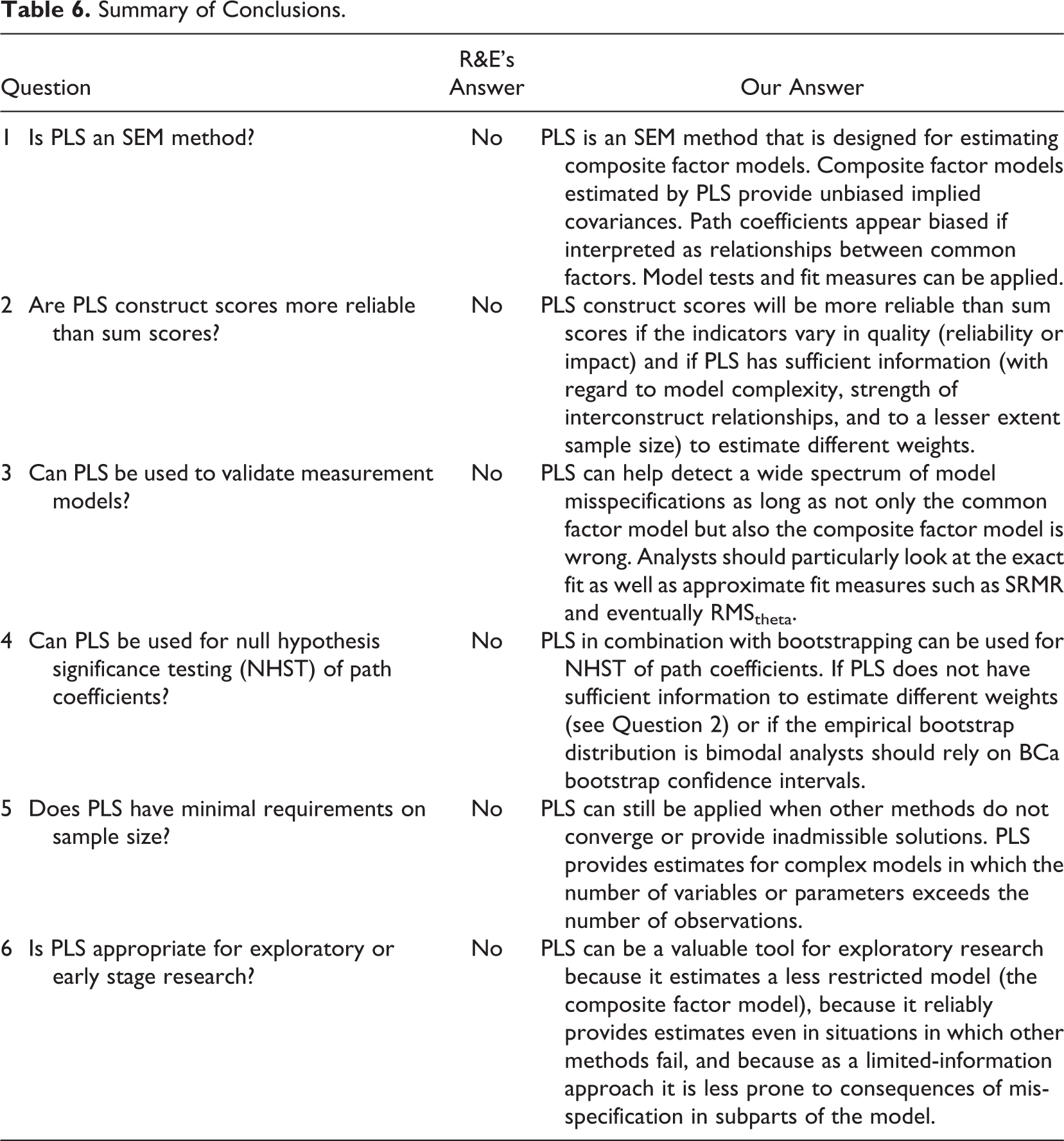
R&E issued six critiques about PLS, which are covered by the following questions: (1) Is PLS an SEM method? (2) Are PLS construct scores more reliable than sum scores? (3) Can PLS be used to validate measurement models? (4) Can PLS be used for NHST of path coefficients? (5) Does PLS have minimal requirements on sample size? and (6) Is PLS appropriate for exploratory or early stage research? Their answer to all these questions is no.

Unlike R&E, we feel that the above questions require more nuanced answers than a simple yes or no. We provide such answers in Table 6 based on our arguments and simulation results.

Table 6.

Summary of Conclusions.

Question		R&E’s Answer	Our Answer
1	Is PLS an SEM method?	No	PLS is an SEM method that is designed for estimating composite factor models. Composite factor models estimated by PLS provide unbiased implied covariances. Path coefficients appear biased if interpreted as relationships between common factors. Model tests and fit measures can be applied.
2	Are PLS construct scores more reliable than sum scores?	No	PLS construct scores will be more reliable than sum scores if the indicators vary in quality (reliability or impact) and if PLS has sufficient information (with regard to model complexity, strength of interconstruct relationships, and to a lesser extent sample size) to estimate different weights.
3	Can PLS be used to validate measurement models?	No	PLS can help detect a wide spectrum of model misspecifications as long as not only the common factor model but also the composite factor model is wrong. Analysts should particularly look at the exact fit as well as approximate fit measures such as SRMR and eventually RMStheta.
4	Can PLS be used for null hypothesis significance testing (NHST) of path coefficients?	No	PLS in combination with bootstrapping can be used for NHST of path coefficients. If PLS does not have sufficient information to estimate different weights (see Question 2) or if the empirical bootstrap distribution is bimodal analysts should rely on BCa bootstrap confidence intervals.
5	Does PLS have minimal requirements on sample size?	No	PLS can still be applied when other methods do not converge or provide inadmissible solutions. PLS provides estimates for complex models in which the number of variables or parameters exceeds the number of observations.
6	Is PLS appropriate for exploratory or early stage research?	No	PLS can be a valuable tool for exploratory research because it estimates a less restricted model (the composite factor model), because it reliably provides estimates even in situations in which other methods fail, and because as a limited-information approach it is less prone to consequences of misspecification in subparts of the model.

The true value of R&E’s article lies not in the answers to the questions it poses but in pinpointing boundary conditions for the use of PLS and detecting weaknesses in some model assessment criteria. At the same time, the contribution of R&E to our understanding of PLS is counterproductive because of the strong assumption that the common factor model is (necessarily) correct, because extant literature was misread or misquoted, and because the results of specific population models were generalized too far. While trying to chase down myths, we argue that R&E have actually created new myths.

There is no such thing as an estimation method that is best for every model, every distribution, every set of parameter values, and every sample size. For all methods, no matter how impressive their pedigree (maximum likelihood being no exception), one can find situations where they do not work as advertised. One can always construct a setup where a given method, any method, “fails.” A (very) small sample or parameter values close to critical boundaries or distributions that are very skewed, thick tailed, and so on, or any combination thereof will do the trick. It is just a matter of perseverance to find something that it is universally “wrong.” A constructive attitude, one that aims to ascertain when methods work well, how they can be improved, and where they complement each other would seem to be more conducive to furthering the scientific enterprise.

An objective critique of any method should not only focus on its limitations but also highlight its advantages. R&E’s analysis falls short here in that it does not mention any of those characteristics that make PLS attractive for researchers. There are many more important questions about the behavior of PLS that deserve scholarly attention, such as these: “How well can PLS predict?” and “How well does PLS perform if the composite factor model is indeed correct?” Preliminary findings give rise to optimism for both these questions: PLS serves well for predictive purposes (Becker, Rai, & Rigdon, 2013), and when the composite factor model is true, PLS clearly outperforms covariance-based SEM and regression on sum scores (Rai et al., 2013). In conclusion, PLS is not a panacea, but certainly an important technique deserving a prominent place in any empirical researcher’s statistical toolbox.