Sage Journals: Discover world-class research

Abstract

We present a thorough performance and energy consumption analysis of the LULESH proxy application in its OpenMP and MPI variants on two different clusters based on Intel Ice Lake (ICL) and Sapphire Rapids (SPR) CPUs. We first study the strong scaling and power consumption characteristics of the six hot spot functions in the code on the node level, with a special focus on memory bandwidth utilization. We then proceed with the construction of a detailed Roofline performance model for each memory-bound hot spot, which we validate using hardware performance counter measurements. We also comment on the observed discrepancies between the analytical model and the observations. To discern the influence of the programming model from the influence of implementation of the code, we compare the performance of OpenMP and MPI based on problem size, examining if the underlying implementation is equivalent for large problems, and if differences in overheads are more significant at smaller problem sizes. We also conduct an analysis of the power dissipation, energy to solution, and energy-delay product (EDP) of the hot spots, quantifying the influence of problem size, core and uncore clock frequency, and number of active cores per ccNUMA domain. Relevant energy savings are only possible for memory-bound functions by using fewer cores per ccNUMA domain and/or reducing the core clock speed. A major issue is the very high extrapolated baseline power on both chips, which makes concurrency throttling less effective. In terms of energy-delay product (EDP), on SPR only memory-bound workloads offer lower EDP compared to Ice Lake.

Keywords

Roofline model performance power dissipation energy consumption LULESH proxy application ice lake and sapphire rapids processors

1. Introduction and related work

As the complexity of modern high-performance computing (HPC) systems continues to grow, achieving optimal performance while minimizing energy consumption has become a paramount challenge for applications in the computational science and engineering field. In this paper, we study the performance and energy of the Livermore Unstructured Lagrangian Explicit Shock Hydrodynamics (LULESH) proxy application Karlin et al. (2012) on multi- core clusters. LULESH is a popular benchmark in the HPC community because of its computational and memory access patterns, which are representative of real-world applications. However, any performance and energy optimization effort requires a thorough comprehension of the interplay between hardware architecture and application behavior. Therefore, this work uses the Roofline Model Williams et al. (2009) to derive performance limits and computational intensities of LULESH on two different clusters based on Intel Ice Lake (ICL) and Sapphire Rapids (SPR) CPUs. Additionally, given the growing emphasis on energy-efficient computing in modern HPC systems, we extend our study to include an energy analysis. Our work offers valuable insights into how LULESH application performance and energy usage can be balanced to achieve better resource efficiency.

1.1. Related work

Previous studies on LULESH have mostly concentrated on performance evaluation Carothers et al. (2017); Malony et al. (2020); Copik et al. (2021) and optimization León et al., 2015, 2016a; Liu and Kulkarni, 2015; Singanaboina et al., 2024, while some efforts have been made to incorporate energy efficiency analysis León et al. (2016b); Wu et al. (2017). LULESH has been extensively studied on GPUs, where works by Williams et al. (2010) and Stratton et al. (2013) show significant speedups on Nvidia K80 and V100 GPUs, with analyses of power and energy trade-offs. Jin and Finkel (2019) compare these to FPGA implementations, demonstrating better energy efficiency of FPGAs for memory-bound kernels. On ARM-based clusters, Chishti et al. (2020) and Ibrahim et al. (2021) investigate energy-efficient heterogeneous systems combining ARM CPUs with GPUs and FPGAs, highlighting their potential for low-power scientific computing. Further, Karlin et al.

Karlin et al. (2013) compared different implementations of LULESH to determine the benefits and drawbacks of various programming models for parallel computation in terms of programmer productivity, performance, and ease of applying optimizations. Marques et al. Marques et al. (2017) demonstrated the usefulness of a cache-aware diagnostic Roofline Model analysis within Intel Advisor ¹ by analyzing LULESH to identify the critical bottlenecks. Nevertheless, to the best of the authors’ knowledge, no prior effort has yet been made to describe the LULESH application using predictive white-box analytic performance models such as Roofline. Additionally, a comprehensive study of the energy aspects of LULESH on contemporary multi-core clusters is still lacking.

1.2. Contribution

This paper makes the following relevant contributions, which, although currently presented only for Intel-based clusters, offer metrics and analysis techniques that are valuable in a larger context.

• We present an overview of performance and energy metrics of LULESH in MPI and OpenMP modes at the ccNUMA domain, node, and multi-node levels on two clusters featuring different generations of modern Intel server CPUs. This comparison underscores the need to balance performance and energy consumption when optimizing parallel applications like LULESH.

• We provide a predictive Roofline performance model for five of LULESH’s hot spot functions for the first time and validate it using hardware performance counter measurements.

• Through kernel-based analysis, we demonstrate that analyzing power dissipation and energy consumption requires a clear distinction between memory-bound and non-memory-bound kernels, the latter being the target for in-core optimizations such as SIMD vectorization and the former offering lower energy- delay product (EDP) on SPR compared to ICL.

• Using the full application, we compare the perfor- mance of OpenMP and MPI across problem sizes to discern the influence of the programming model from the influence of code implementation.

• We further show that the minimization of energy-delay product and energy to solution are dominated by code scaling characteristics and chip idle power, making concurrency throttling² and the uncore clock speed settings less effective while core clock speed settings play a more significant role in improving efficiency.

The LULESH application was chosen because of its nontrivial combination of memory-bound and non-memory-bound hotspots, which also have different characteristics in terms of power and energy consumption. Most Roofline case studies (see, e.g., Marques et al., 2017; Calore et al., 2020) conduct an empirical analysis, measuring the computational intensity and performance per hotspot and putting dots in a Roofline plot; here we conduct a predictive analysis and compare it with the empirical data, which results in improved insight. Z-plots are employed for the energy analysis. Both analyses can be used as starting points for performance and energy optimizations. In a nutshell, since most of the hotspots are memory bound and our analysis provides best- and worst-case predictions for the computational intensity, memory traffic reductions (if possible) will be most beneficial for performance while the impact of vectorization will be limited. In terms of energy and EDP, clock speed reduction has more impact than concurrency throttling due to the high (zero-core) baseline power of the CPUs under consideration.

We restrict ourselves to two Intel-based platforms in order to enable an in-depth study of the intricate performance and power properties of LULESH and to provide some insight into the evolution of Intel server CPUs. A thorough cross-platform investigation of performance and power for LULESH is left for future work.

1.3. Overview

This paper is organized as follows: We first provide an overview of our experimental environment and methodology in Sect. 2, followed by an introduction to the LULESH proxy application and its implementation details in Sect. 3. In Sect. 4 we concentrate on performance, power, and energy by carrying out a kernel-based analysis on the node level and constructing a Roofline performance model in Sect. 4. Section 6 extends the analysis to the full application for both single- and multi-node scenarios. Finally, Sect. 7 summarizes the paper and gives an outlook to future work.

2. Test bed and experimental methodology

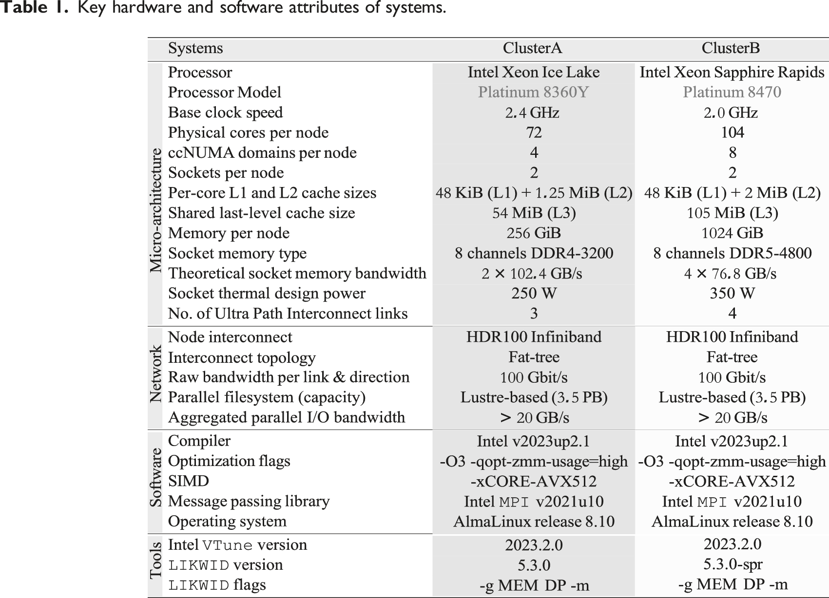
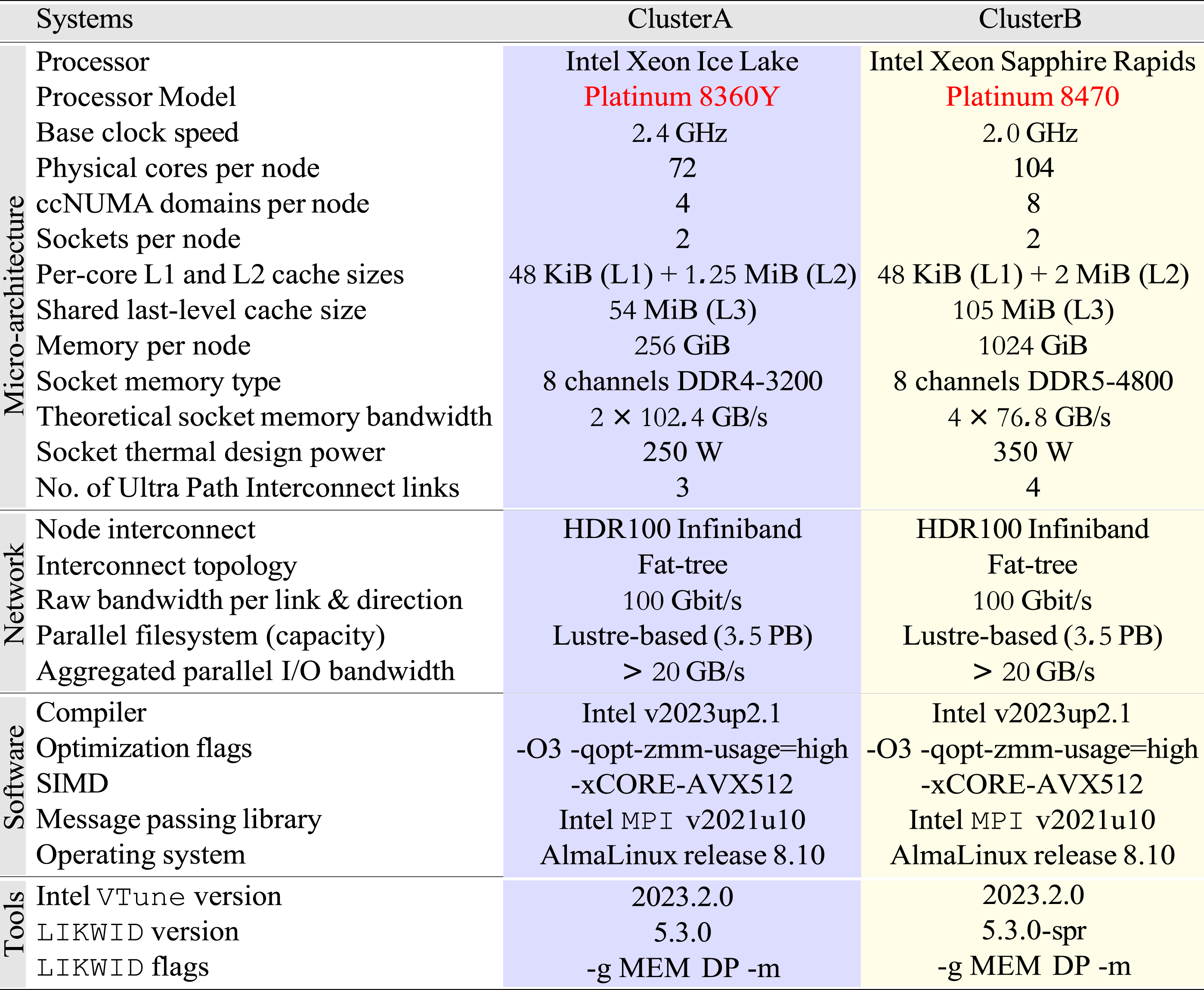
Table 1 outlines the hardware and software configurations employed for our experiments. We used the following two Intel-based InfiniBand (HDR-100) clusters³:

(1) ClusterA comprises two Intel Xeon Ice Lake (ICL) CPUs per node, each with 36 cores.

(2) ClusterB comprises two Intel Xeon Sapphire Rapids (SPR) CPUs per node, each with 52 cores.

Table 1.

Key hardware and software attributes of systems.

Sub-NUMA Clustering was enabled on both systems, leading to a fundamental scaling unit (i.e., one ccNUMA domain) of half (i.e., 18 cores) of ClusterA’s socket on and one-fourth (i.e., 13 cores) of ClusterB’s socket. All hardware prefetching mechanisms were enabled, and hyper-threading was disabled on both clusters. Consecutive OpenMP threads and MPI processes were mapped to consecutive cores using the likwid-perfctr and likwid-mpirun Treibig et al. (2010) startup wrappers, respectively. We did not test the HBM variant of Sapphire Rapids CPUs as it was not generally accessible at the time of writing.

Unless otherwise specified, the core clock frequency was fixed to the base values of the respective CPUs via the Slurm batch scheduler (cpu-freq=<min freq in kHz>-<max freq in kHz>:performance), avoiding any power-saving behaviors that would typically lower the frequency. Whenever applicable, the uncore and turbo clock frequencies of the hardware were set using the likwid-setFrequencies tool. The expected clock frequency settings were verified using likwid-perfctr.

The Intel VTune Profiler⁴ and the LIKWID tool suite⁵ were employed for reading hardware performance and energy counter measurements and validating results where necessary. The analyses from Likwid and Vtune yielded comparable values; thus, we focus on reporting the results from Likwid. The likwid-powermeter tool was utilized to obtain theoretical insights on turbo mode. Given the 1 kHz update frequency of RAPL counters on ICL and SPR, we excluded measurements shorter than a few milliseconds to ensure accuracy. All node-level experiments were conducted on the same node to reduce RAPL measurement variation across nodes. Before collecting measurements, a few warm-up time steps were performed to stabilize runtime and eliminate first-call overhead. To account for runtime variability, we repeated each code execution multiple times, and only statistically significant deviations were reported. We present results for Intel MPI implementation, as node- level findings with OpenMPI implementation showed only minor differences.

2.1. Observables for analysis

The performance metric used is the Figure of Merit (FOM), defined as the number of elements solved (z) per second (s). Alternative metrics, though ignored here, are the wall-clock time (complete run time) and the grind time (run time to update a single zone for one iteration). We focus on metrics such as memory bandwidth utilization, overall instructions per work, power dissipation, energy-to-solution per work, and the energy-delay product for both CPU and DRAM. These metrics help quantify the impact of factors like problem size, core and uncore clock frequency, number of active cores per ccNUMA domain, and number of nodes. The merit of normalizing metrics by work, rather than using raw metric, ensures comparability across problem sizes and weak scaling scenarios.

2.2. Open-source dataset artifact

All information required to reproduce the data in this work is available at https://github.com/RRZE-HPC/LULESH-AD⁶ Afzal et al. (2025). Reproducibility initiative dependencies provided by the repository include a comprehensive description of all data sets and figures. These descriptions include machine state files that document the hardware and software environments, scripts that explain the experimental design and methodology, modified code that incorporates LIKWID markers, and supporting data for experimental results.

3. Livermore unstructured lagrangian explicit shock hydrodynamics (LULESH)

3.1. Introduction

LULESH is a MPI- and OpenMP-parallel proxy application developed by Lawrence Livermore National Laboratory (LLNL) for shock hydrodynamic simulation on unstructured grids. Originally, it was designed to simplify the complex structure of a real application while retaining the typical characteristics of computational workload encountered in real-world shock hydrodynamics problems. It is a multi- phase code whose functions have various computational and communication requirements. It employs an explicit time integration method and partitions the spatial problem domain into multiple volumetric elements of the mesh to discretely estimate the hydrodynamic equations. Functions are called on a region-by-region basis to make the memory access patterns non-unit stride and to allow for configurable artificial load imbalance for evaluation purposes. The mapping between materials and regions is crucial in LULESH, where multiple materials are mapped onto multiple regions (subsets of the mesh) of varying sizes, all modeling the same ideal gas material. This uneven distribution of regions and different amounts of computation per grid point might cause a load imbalance. LULESH models how the material deforms over time under shock and employs the Lagrangian approach, where the computational mesh moves with the material. This approach allows for the explicit tracking of density, pressure, and internal energy.

3.2. Implementation

The LULESH algorithm, outlined in Table 2, is implemented in C++. Although the LULESH code uses a Cartesian mesh (more specifically, cubes), it mimics the unstructured, complicated hexahedral mesh geometry by employing indirection arrays and an unstructured data layout. Two stages are involved in updating the physical quantities: first, the nodal updates at the hexahedra’s corners, and then, the element updates at each hexahedra’s center. Positions and velocities are stored by nodes, while energy and pressure are stored by elements. The first step of nodal updates entails computing the nodal forces from the elemental contributions of volume force and stresses, which is the most computationally demanding step. Then, it performs a diagnostic check for negative volumes, and each nodal force element-wise receives an hourglass contribution. To calculate new nodal velocities and positions, it further computes the accelerations with appropriate symmetry boundary conditions. The first step of element updates entails the calculation of elemental kinematic values and new elemental and regional artificial viscosities. After that, material properties are applied to each element, and the Equation of State (EOS) is evaluated. Then, material properties are applied to each element and the Equation of State (EOS) is evaluated. An outer loop over the regions and an inner loop over the elements in a region are used in the implementation. The communication of ghost fields happens twice in the code. First, the communication happens for the positions exchange to ensure the same nodal values of the neighboring elements. Second, viscosity gradients are exchanged following their computation.

Table 2.

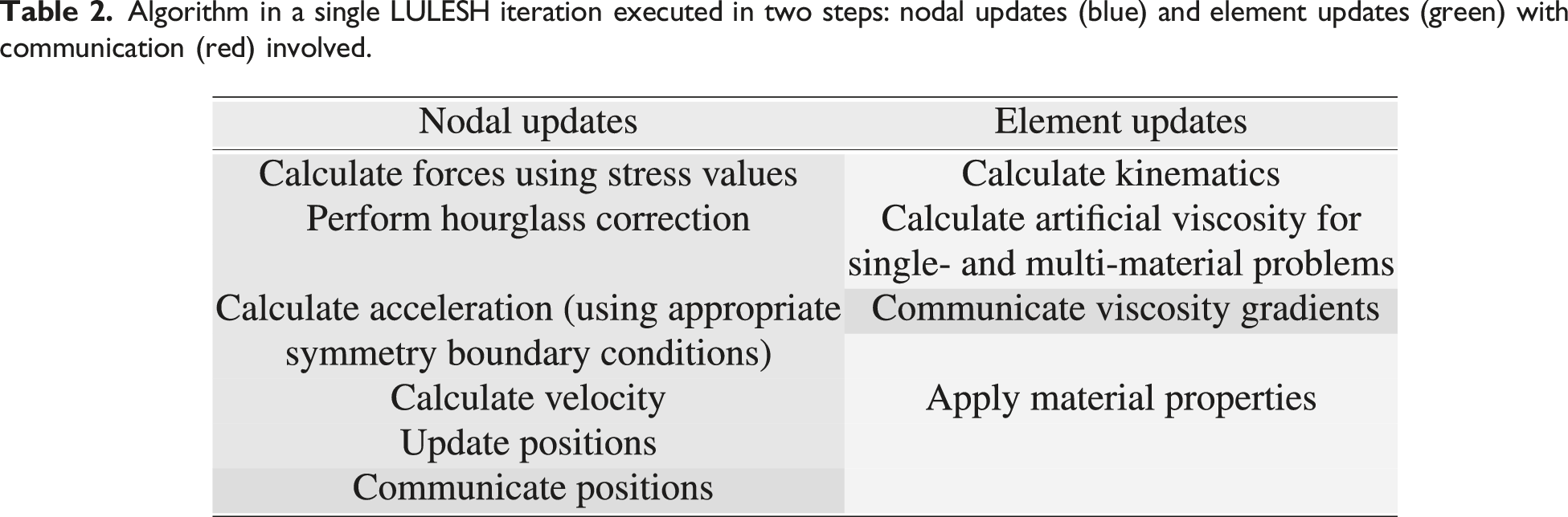
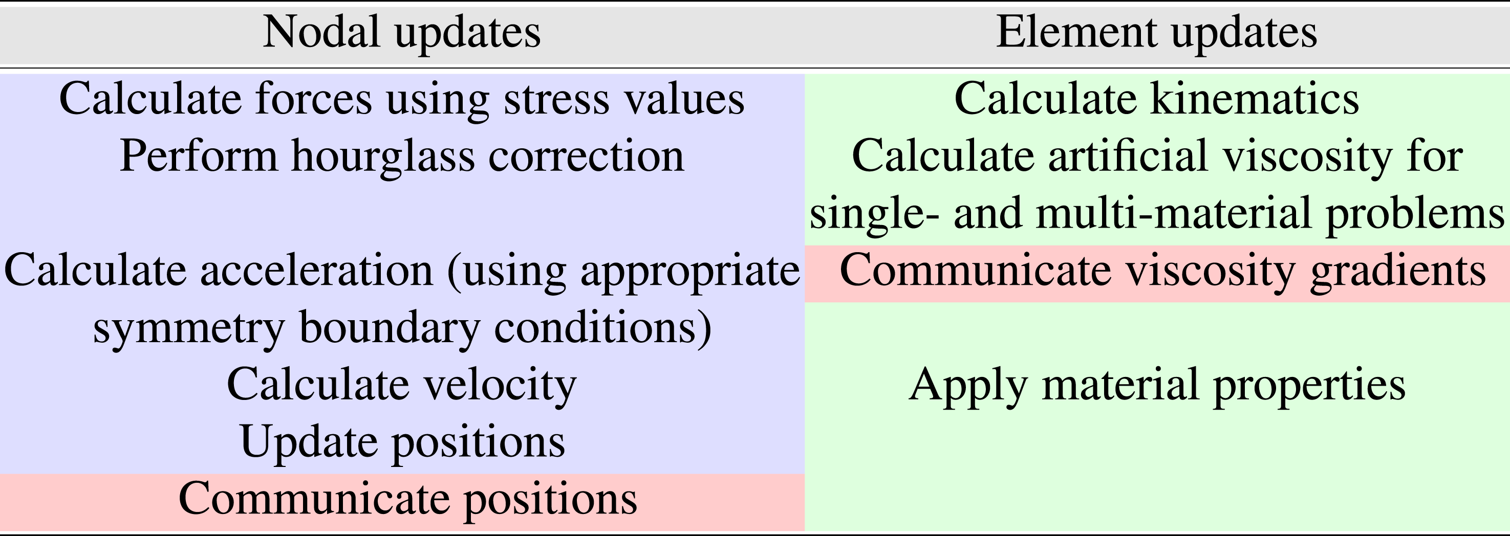
Algorithm in a single LULESH iteration executed in two steps: nodal updates (blue) and element updates (green) with communication (red) involved.

3.3. LULESH Configuration settings

This study used the first official release (version 2.0) of the LULESH proxy application⁷ Karlin et al. (2012), which, by default, calculates time constraints (courant and hydro) and determines the minimum time step required across domains. This dynamic time step calculation incurs extra reductions (MPI_Allreduce via the MPI MIN operation) during domain.cycle one iterations, which are only necessary to enforce time constraints. The number of steps to solution scales to an arbitrary size based on an analytical equation. Independent of the time step size, we used a fixed iteration count of 300 (domain.cycle in code and -i on the command line). The domain size was varied from 60³ to 350³ for the OpenMP version and from 60³ to 150³ per process for the MPI version (numElem in code and -s on command line). In the MPI parallelization of LULESH using a weak scaling approach, the total problem size is defined as ps³, where p represents the number of MPI processes (required to be a cubic number), and s denotes the domain size per process. For larger domain sizes, the working sets were at least 10 times larger than the last-level cache of a single chip, preventing the working set from fitting into the available cache⁸. Load imbalance, which is enabled by default, was disabled by setting the cost (-c) and balance (-b) command-line options to zero. The number of regions is highly problem dependent, and at a minimum, it must equal the number of distinct materials. Therefore, we used 11 distinct regions, as defined by default. The message profile indicates long-distance point-to-point communication is used, involving the MPI_Isend, MPI_Irecv, MPI_Wait, MPI_Waitall sequence. We consistently applied the -O3 optimization and the widest supported SIMD instruction set, specifically -xCORE-AVX512 -qopt-zmm-usage=high, supported by the Intel architectures. For data taking with likwid-perfctr, the LIKWID marker API was included in the code to allow separate measurement on each loop of the hot spot functions.

4. Breakdown analysis with profiling

This section offers basic insights into the performance, power, and energy-to-solution characteristics of hot spots within LULESH through profiling. We compare the OpenMP- and MPI-parallelized versions of the code on two clusters featuring Intel Ice Lake and Sapphire Rapids CPUs. The focus of hot spot analysis is to examine the differences in performance and energy behavior between scalable and non-scalable functions. In addition, Section 6 provides a comprehensive performance analysis for the full application, which includes a mix of memory-bound and non-memory-bound functions.

4.1. Hot spot functions

Most of the runtime of the application is in 22 compute kernels; we instrumented these using the LIKWID marker API. Among these, the following six are primary hot spot functions: CalcHourglassControlForElems, CalcFBHourglassForceForElems, IntegrateStressFor-Elems, CalcKinematicsForElems, CalcMonotonicQGradientsForElems, and EvalEOSForElems.

4.2. Performance

In Figure 1(a), the 22 functions are listed in the legend in descending order based on their serial runtime at a problem size of 350³, with the remaining application runtime placed at the end. For both OpenMP and MPI, the 22 kernels account for 90% of total application runtime on ICL and 87% on SPR. Among them, six primary hot spot functions contribute 76% of the application’s overall runtime on ICL and 73% on SPR. More specifically, six hot spot functions take {16.4,16.2,14.6,14.3,7.9,6.8} percent of overall application runtime in order on the OMP-ICL version. However, the values for the other three variants are comparable, ranging from 6% to 16%.

Figure 1.

Runtime breakdown of 22 LULESH functions on a single core for (a) four code variants at 350³ domain size and (b, c) varying domain sizes for six hot spot functions in OMP-ICL and MPI-ICL versions.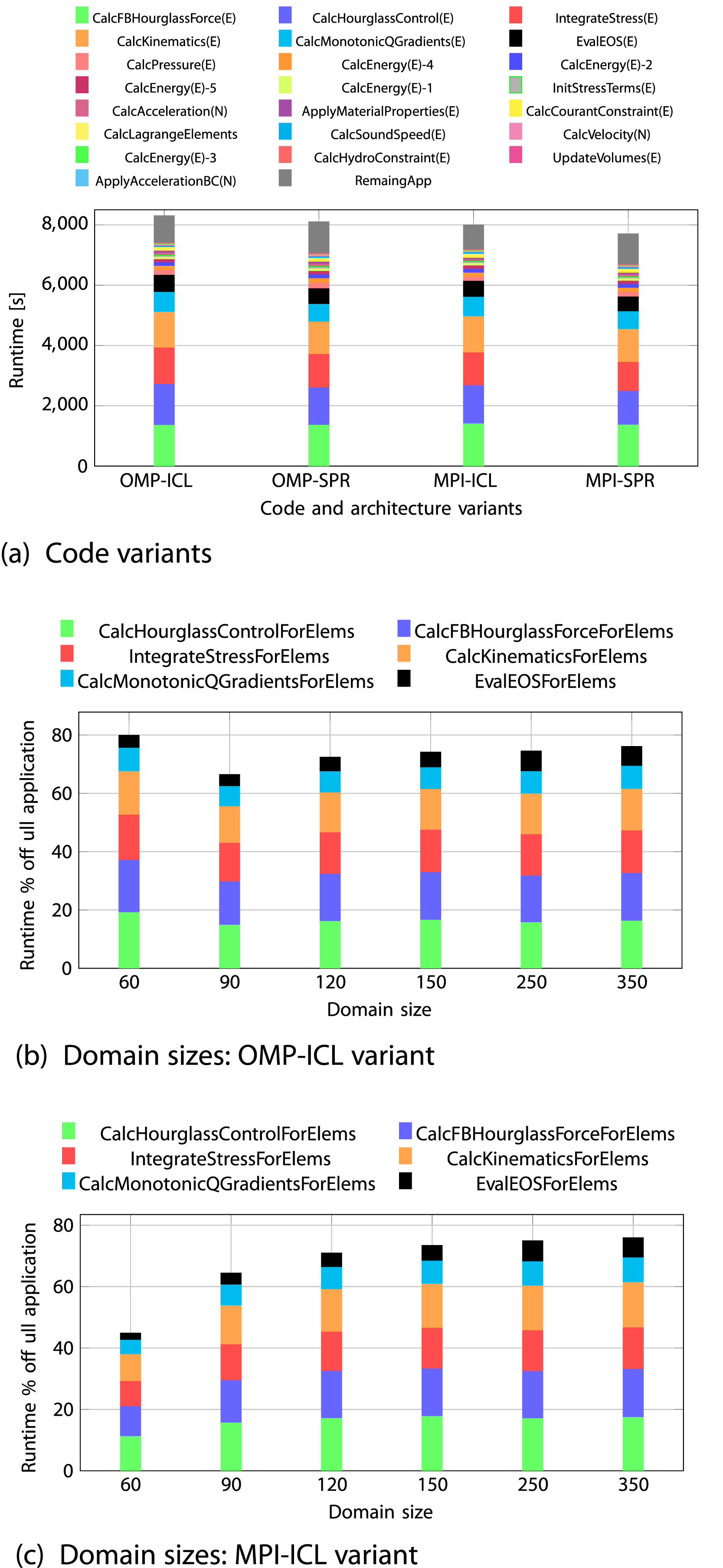

Figure 1(b) and (c) show the percentage of runtime relative to the full application for the six most relevant hot spots with varying problem size. For large problems, these fractions are very similar between MPI and OpenMP, while there are significant differences at smaller problem sizes. The runtime fractions relative to the 22 functions for the six hot spot functions remains unchanged (consistently accounting for 90%) across all problem sizes.

In order to discern memory-bound from non-memory-bound functions, we measured the memory bandwidth separately for the 22 hot spot kernels and present the data for the six most relevant hot spots in Figure 2(a) and (d). In the OpenMP version, only one out of 22 functions, CalcKinematicsForElems, is non-memory-bound. In contrast, the MPI version has five non-memory-bound functions, including two hot spot functions (CalcKinematicsForElems, IntegrateStressFor-Elems) and three non-hot spot functions (CalcCourantConstraintForElems, CalcHydroConstraintForElems, UpdateVolumesForElems). Figure 2(a) also shows that a few functions exhibit significant superlinear scaling when going from one to two cores. Although the full MPI application on a single core overall executes faster than any OpenMP version (OMP-ICL and OMP-SPR), the two non-memory-bound hot spot functions in the MPI version take slightly longer to execute.

Figure 2.

Performance-energy trade-offs for six LULESH hot-spot functions, presented for both OpenMP (top) and MPI (bottom) versions on the ICL-based ClusterA node (subplot view in each plot: SPR-based ClusterB). The domain sizes have been selected as 350³ for OpenMP and 150³ for MPI. On the x-axis, 18 cores (representing one ccNUMA domain) are allocated for OpenMP (top row), while 64 cores (arranged in a cubic configuration, representing the total number of cores available on a single node) are allocated for MPI (bottom row). The plots illustrate: (a, d) bandwidth, (b, e) total power, and (c, f) a z-plot showing total energy-to-solution versus performance. The z-plot highlights the optimal EDP for different core counts and core frequencies (ranging from 1.0 to 2.8 GHz) at two corner cases: memory-bound hot spot function 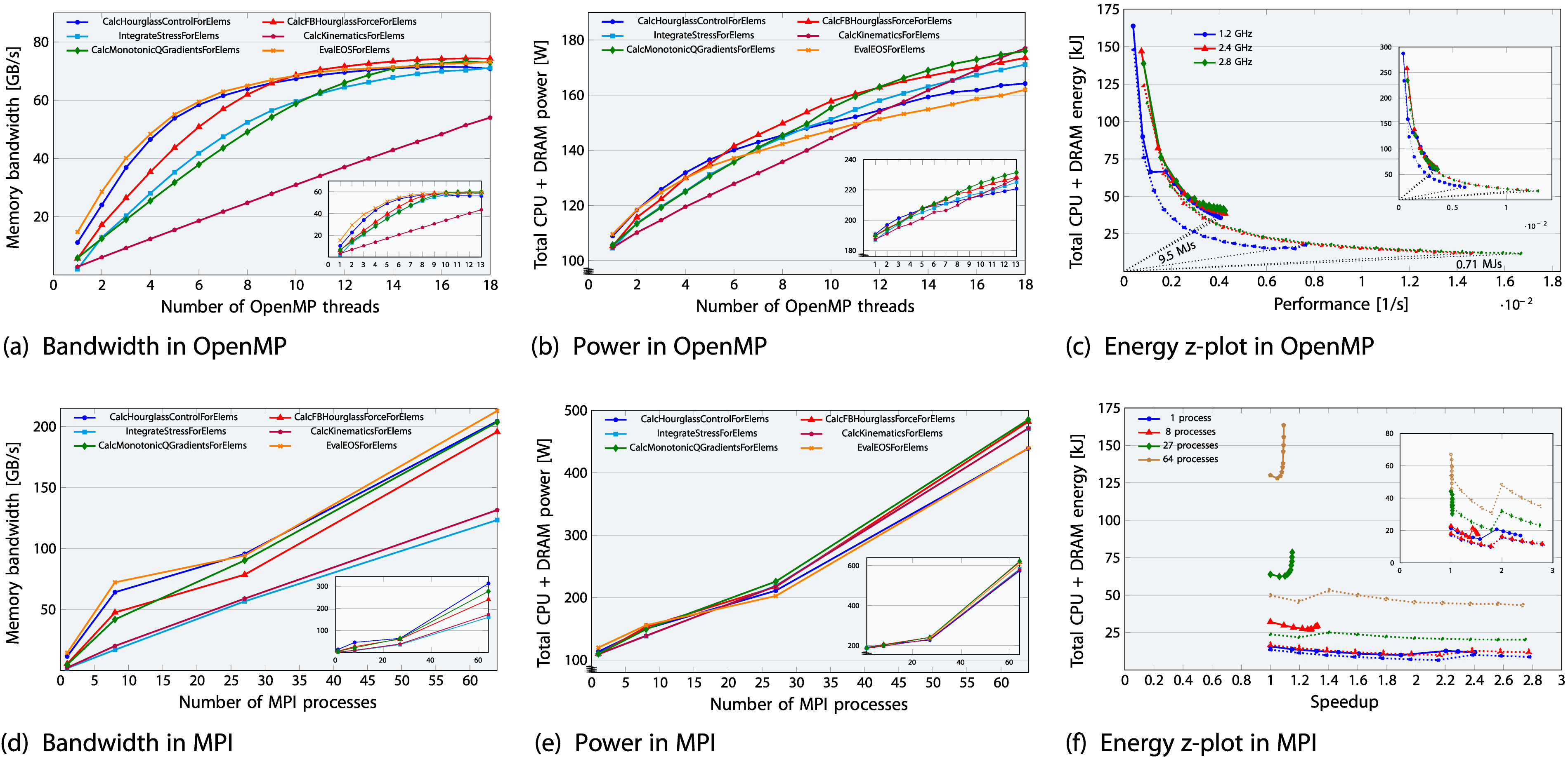CalcHourglassControlForElems (solid) and non-memory-bound hot spot function CalcKinematicsForElems (dotted).

Upshot: LULESH shows a mix of memory-bound and non-memory-bound hot spot functions, which behave in accordance with expectations. The hot spot function contributions are similar between OpenMP and MPI, though four memory-bound functions in OpenMP show scalable behavior in MPI, including one hot spot function.

4.3. Power, energy-to-solution and EDP

Figure 2(b) and (e) shows that the total CPU and DRAM power dissipation of the hot spot functions (162–177 W for OMP-ICL on one ccNUMA domain and 439–485 W for MPI-ICL on 64 cores) eventually lies within the power range of the entire LULESH application (170 W for OMP-ICL and 451 W for MPI-ICL, which will be discussed later in Figure 5). When comparing memory-bound functions with the non-memory-bound function, the scalable function (purple) exhibits a distinct power pattern: it begins with low power at one core, aligning with other non-scalable functions, and then increases linearly as scaling progresses, ultimately reaching the highest power level among all functions across the full ccNUMA domain due to significant usage of memory bandwidth and in-core resources. However, the non-scalable functions saturate more quickly with the number of cores, causing them to heat up faster.

In Figure 2(c) we present a z-plot Afzal (2015); Wittmann et al. (2016) with energy on the y-axis, performance on the x-axis, and the number of cores as the parameter along the data sets for the OpenMP version at a problem size of 350³. In a z-plot⁹, horizontal and vertical lines indicate constant energy and performance, respectively. If the problem size is constant, each line through the origin is the locus of constant energy-delay product (EDP, the product of energy to solution and runtime), and its slope is proportional to the EDP. Optimizing for EDP is thus a search for the point in the z-plot that lies on the smallest-slope EDP line. For brevity, we present z-plot results for only three frequency settings: at, below, and above the base frequency, i.e., 1.2, 2.4, 2.8 GHz, and for the two functions CalcHourglassControlForElems (solid) and CalcKinematicsForElems (dotted). For comprehensive results on the impact of all frequencies on performance, power, and energy, we refer to of Appendix B Figures 11 and 10. The six hot-spot functions account for 74% (672 kJ out of 905 kJ) of the total energy consumption of the entire application on a single core, and 58% (133 kJ out of 231 kJ) on a single ccNUMA domain. The energy consumption of the scalable function (dotted line in Figure 2(c)) initially aligns with that of the non-scalable function but decreases more sharply as scaling improves. Ultimately, across the full ccNUMA domain, it uses less than half the energy of the CalcHourglassControlForElems function (solid line). This is not surprising since the memory-bound function’s performance saturates at some point; more cores deliver marginally more performance but still increase the power consumption.

Figure 2(c) shows that the non-memory-bound hot spot function attains the lowest EDP with all cores active on the ccNUMA domain and running at a clock speed of 2.8 GHz, clearly exhibiting a “race-to-idle” characteristic. The energy to solution is minimal at this point as well. For the memory-bound hot spot, the situation is not so clear; lowest clock speed clearly entails lowest energy to solution, but there is little variation in the EDP in the range between 1.2 and 2.4 GHz, and due to the dominating baseline power all cores must be used. However, concurrency throttling (using fewer cores) for memory-bound code could become effective if non-compact pinning is used instead. In memory-bound functions, playing with frequency does not impact performance very much, but it does make a difference with respect to energy. On the other hand, in compute-bound scalable kernels, all that matters is frequency and number of cores. There is a minimum energy point with respect to clock frequency which is usually far away from the performance maximum. At frequencies below the base frequency, a kink appears at a certain core count, becoming more pronounced for memory-bound kernels and less so for non-memory-bound kernels and full applications, which include a mix of both kernel types. This is due to a peculiar behavior of the uncore frequency with changing number of cores at core frequencies below the base value; full data is available in the appendix.

In the subplot inserts of Sapphire Rapids, compared to Ice Lake, its significantly higher baseline power reduces the distinction between power trends of scalable and non-scalable hot spots and makes energy to solution slightly severe for memory-bound kernels. However, as the scale reaches a full node, the energy to solution becomes comparable to ICL, resulting in a higher EDP on SPR, as shown later in Figure 5.

In Figure 2(f) we show a z-plot for the MPI version at a problem size of 150³ per process with clock frequency as a parameter along each data set. On the x-axis we choose speedup as a metric since the problem size changes for changing MPI process counts (1, 8, 27, 64). The data shows again the qualitative difference between memory-bound and non-memory-bound kernels. For memory-bound kernels, performance gains cease beyond 1.4 GHz if most of a socket is utilized; any frequency increase beyond this point merely results in wasted energy without further performance benefits.

Upshot: The six hot spots fall in the same power range as the full application, consuming up to 58% of the overall energy to solution at large problem sizes. The best frequency setting for optimal EDP differs significantly between scalable and non-scalable hot spots, but the base frequency of the chip is a good overall compromise.

5. Analytic performance modeling

In this section, we construct and validate memory traffic models for the memory-bound hot spots found in the LULESH application.

5.1. Computational intensity

The computational intensity I of a loop is the ratio of the number of floating-point operations N_F to the data transfers to and from main memory in bytes, calculated as follows: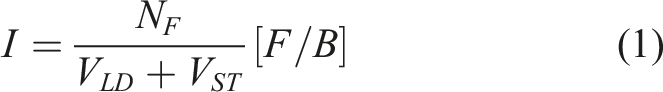

I = \frac{N_{F}}{V_{L D} + V_{S T}} [F / B]

(1)

Where V_LD and V_ST are the load and store data volumes, respectively. For LULESH, we compute the computational intensity for each loop and compare it with the values obtained from hardware performance counters. For our calculations, we consider the flop or byte count for one iteration of the outer loop, which has a loop length of “numElem” (representing the amount of work per domain; -s). For example, at a cubic domain of size 350, “numElem” is 350³.

The two primary data structures used in the hot-spot functions of LULESH are Real_t (double) for double-precision floating-point numbers and Index_t (int32_t) for 4-byte signed integers. Since the compiler may optimize or modify arithmetic expressions, counting the number of FLOPs manually is not reliable. Instead, we use the more accurate FLOP count provided by tools like LIKWID. This ensures a more precise analysis, as LIKWID directly counts FLOPs at the hardware level, reflecting any optimizations that may be applied by the compiler. Further, for the load and store volume calculation, we compare the manual prediction against the measured load and store traffic in memory using LIKWID. This comparison helps verify whether factors such as data reuse and write-allocate behavior play any role. For a fair comparison, we use -qopt-streaming-stores=never to disable streaming stores.

5.1.1. Common functionality among three hot spots

Before diving into a detailed discussion of the five memory-bound hot spot functions, we begin by calculating the data transfers involved in the common functionality shared by the first, third, and fourth hot spot functions. At the beginning of these three functions, domain.nodelist(i) retrieves node indices for each element (line 4 of Listing 2, line 3 of Listing 5 and line 5 of Listing 8) and loads the corresponding nodal coordinates from global arrays into local arrays using the CollectDomainNodesToElemNodes function (line 5 of Listing 2, line 4 of Listing 5 and lines 6–9 of Listing 8). The expression domain.nodelist(i) yields a 4-byte index of eight consecutive nodes, which gets assigned to elemToNode. In Listing 1, the CollectDomainNodesToElemNodes function then loads eight 4-byte indices from main memory, resulting in a total load of 32 bytes (lines 2–3). Each set contains eight elements, each eight bytes long, leading to a total of 8x24 bytes for loading the positional coordinates (domain.x, domain.y, and domain.z) in lines 4–5. The index values nd0i, nd1i, nd2i, nd3i, nd4i, nd5i, nd6i, nd7i and elements elemX, elemY, elemZ, are updated and reused for the next iteration. In the best case, these data transfers can then come from cache.

Listing 1. The CollectDomainNodesToElemNodes function is called in three hot spot functions.

Listing 2. CalcHourglassControlForElems hot spot function.

Listing 3. The VoluDer function is called 8 times through line 6 of the CalcHourglassControlForElems function.

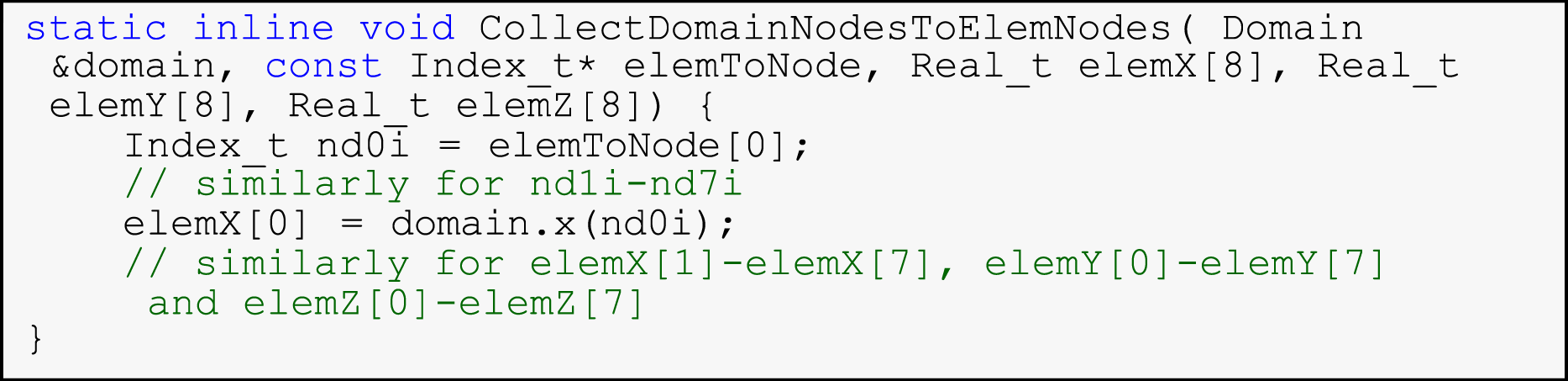
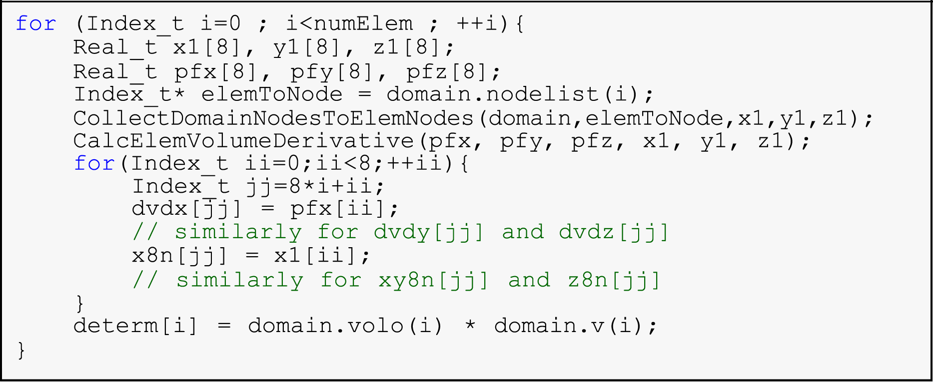
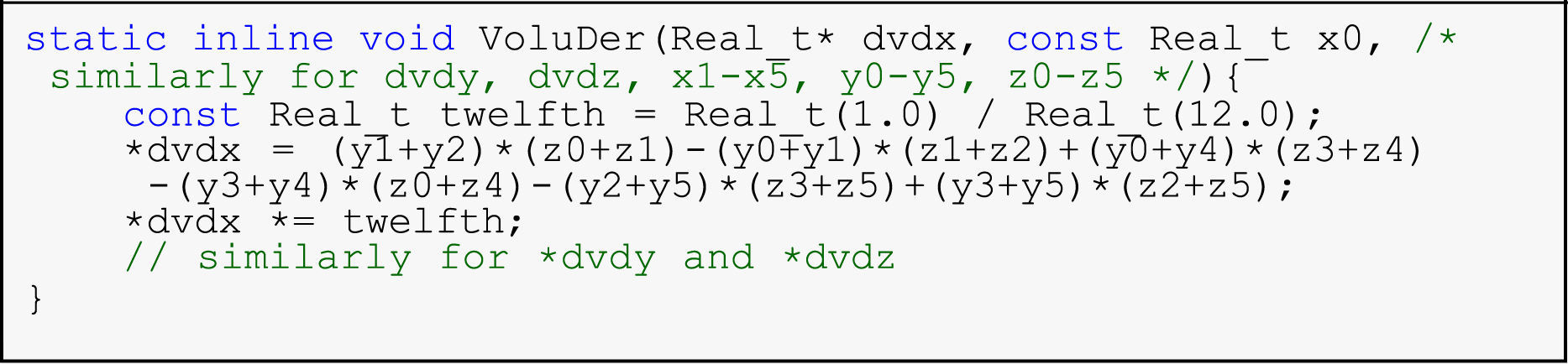
5.1.2. Function CalcHourglassControlForElems

This first hot spot function, presented in Listing 2, calculates the standard hourglass force based on the element’s geometry and deformation. It processes elements within the domain, with data transfers involving 228-byte loads (lines 4–5) as detailed above. In line 6 of Listing 2, the CalcElemVolumeDerivative function calls the VoluDer function (Listing 3) eight times to compute the volume derivatives needed for calculating the volume force contributions to each element, which are then summed with those of its eight surrounding nodes. Without considering compiler optimizations, the source code of this function has a total of 585 floating-point operations. However, the compiler performs substantial rearrangement of the arithmetic expressions, so that the total measured flop count is just 325 (N_F). We will use this number in the analysis. Since the arrays pfx, pfy, pfz, x1, y1, and z1 are declared within the loop (lines 2–3 of Listing 2), they incur no data traffic from main memory.

In lines 7–13 of Listing 2, each iteration of the outer “for-loop” involves six arrays {dvdx, dvdy, dvdz} and {x8n, y8n, z8n}, each of length eight times the number of elements. These arrays are used to temporarily store volume derivatives and coordinates, respectively, which are later passed to the subsequent CalcFBHourglassForceForElems function. This results in a data transfer of 8x48 bytes each for stores and loads due to write allocation. Additionally, line 14 of Listing 2 requires a data transfer of 8 bytes to store data for determ[] and 24 bytes for loading data for three arrays (domain.volo, domain.v and determ[]). In the parallel multi-threaded case on a ccNUMA domain, the intensities slightly worsen due to marginally higher memory traffic.

The predicted and measured computational intensities, presented in Table 3, are similar. The slight discrepancy in measured memory traffic between SPR and ICL is likely due to the cache reuse for certain arrays.

Table 3.

Single-threaded predicted and measured computational intensities equation (1) in [F/B] for the five memory-bound hot spots. Multi-threaded measured intensity values, scaled to the entire ccNUMA domain in OpenMP, are given in parentheses.

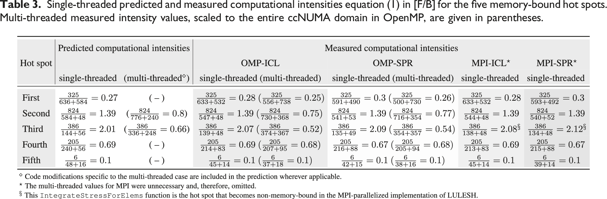
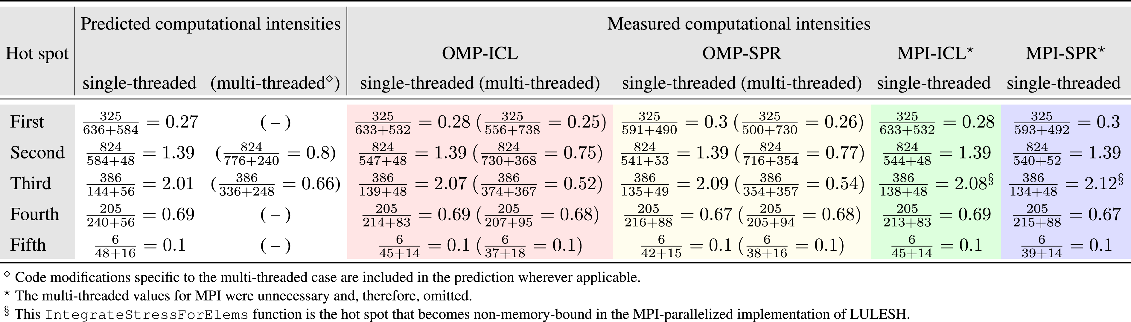
A detailed analysis of the computational intensities for the remaining four functions – CalcFBHourglassForceF-orElems, IntegrateStressForElems, CalcMonotonicQGradientsForElems, and CalcMonotonicQGradientsForElems – is presented in Appendix A, with the results summarized in Table 3.

5.2. Roofline modeling

The Roofline model (P = min (P_peak, I×b_s)) analytically quantifies the hardware-software interaction by relating peak performance (P_peak) and memory bandwidth of hardware (b_s) to computational intensity (I) of a loop. The performance is limited by either P_peak or I ×b_s, indicating compute- or memory-boundedness, respectively.

In Figure 3, two lines are plotted to represent bandwidth, with a band between the minimum and maximum values. A single ccNUMA domain of the Ice Lake (Sapphire Rapids) system has a theoretical memory bandwidth of 102.4 GB/s (76.8 GB/s), with the maximum achievable read-only bandwidth of 90 GB/s (68.5 GB/s) reflecting the most favorable benchmark conditions, while both the update benchmark and LULESH proxy application reach a maximum of 71 GB/s (57 GB/s). Since LULESH is not completely vectorized, the peak performance ceiling of the model is calculated using the scalar limit. The theoretical scalar peak performance for one ccNUMA domain is 172.8 Gflop/s on the Ice Lake system and 104 Gflop/s on the Sapphire Rapids system. Measured performance is plotted since predicted performance always aligns with the bandwidth ceiling, making it unnecessary to plot as a data point. Predicted values are denoted by empty circles, while the filled color circle denotes the measured values obtained from LIKWID. Finding indicates that intensities are fairly predicted and highlights the interaction between computation and memory bandwidth using the Roofline model, where programming model overhead appears as a gap between measured performance and the Roofline limit.

Figure 3.

The Roofline model for the OpenMP-parallelized LULESH application is shown, presenting the measured values for both the full application and individual hot spots (filled circles) against analytical predictions (empty circles). This data is presented for a single ccNUMA domain on two systems: (a) Ice Lake and (b) Sapphire Rapids.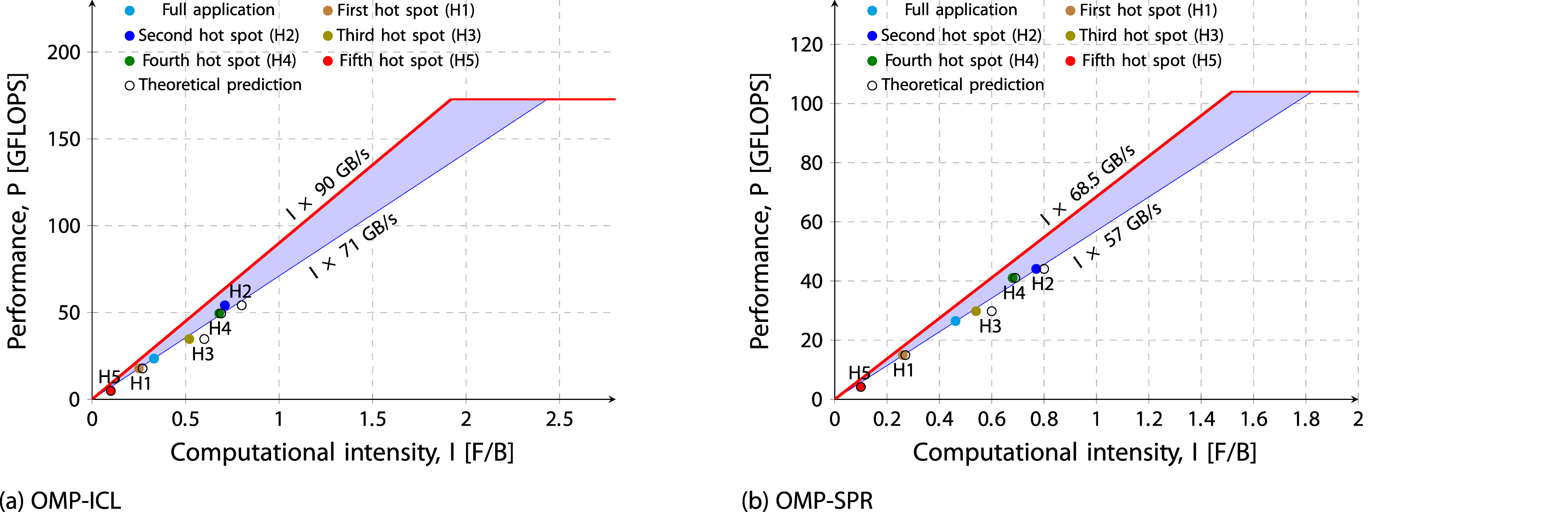

6. Full application analysis

This section evaluates the performance, power, and energy to solution for the full LULESH application on SPR and ICL. The theoretical ratios of peak performance, memory bandwidth, and thermal design power (TDP) for the Sapphire Rapids node compared to the Ice Lake node on the ClusterA are 1.2, 1.5, and 1.4, respectively.

6.1. Domain size impact

On modern architectures, the execution and data transfer features render the LULESH code memory-bound. In Figure 4(a), memory bandwidth increases significantly up to a domain size of 150, after which the increase becomes less pronounced, reaching {49, 56, 62, 66, 70, 71} GB/s (ICL) and {41, 47, 51, 54, 57, 57} GB/s (SPR) for domain sizes of {60, 90, 120, 150, 250, 350}10.

Figure 4.

Performance for the full LULESH application, presented for both OpenMP (top) and MPI (bottom) versions on the ICL-based ClusterA node (subplot view in each plot: SPR-based ClusterB). The plots illustrate: (a) memory bandwidth, (b) performance, and (c) the total number of overall instructions normalized by domain size.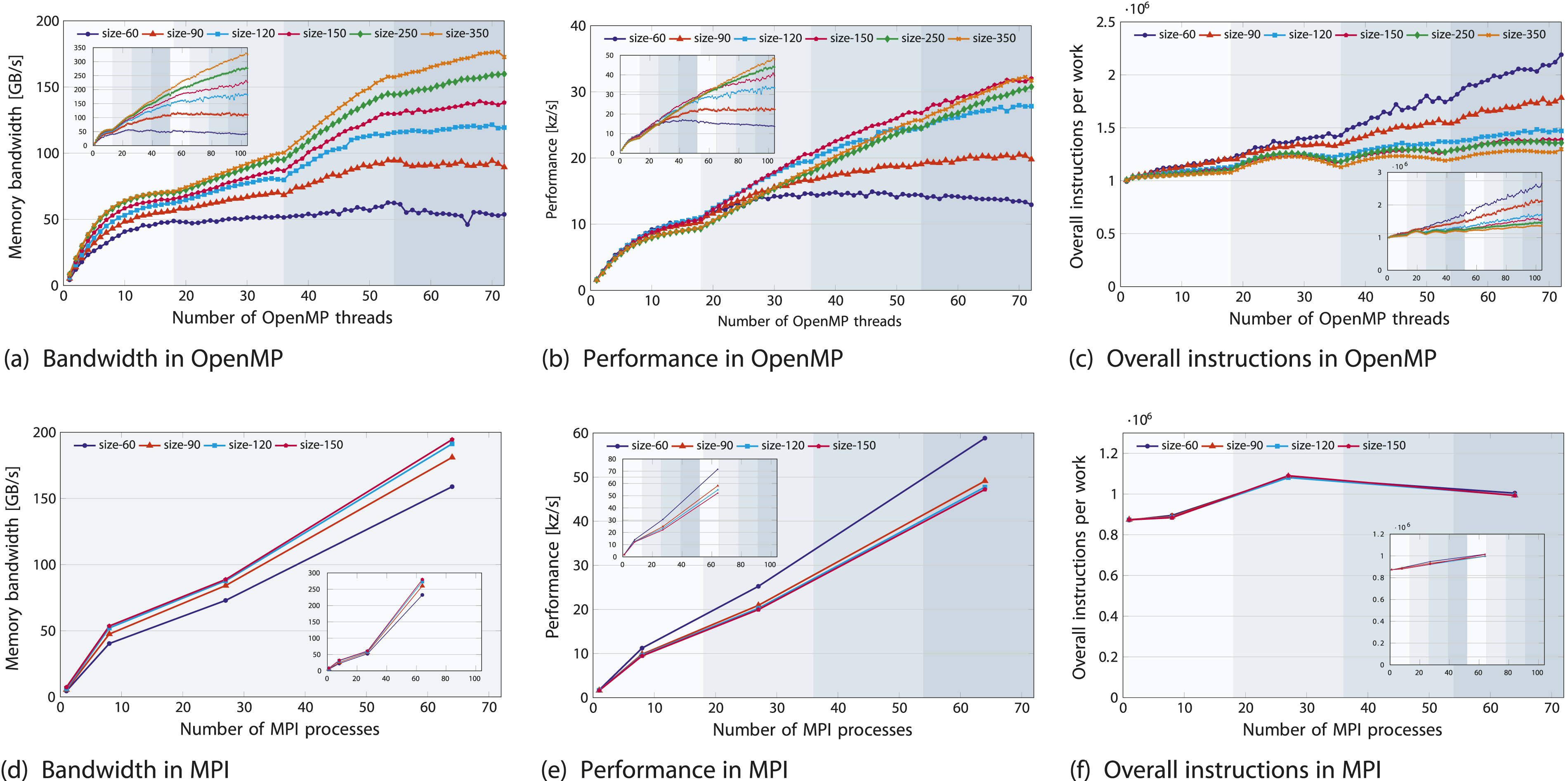

In Figure 4(a) and (b), while memory bandwidth saturates by staying roughly constant towards the end of the ccNUMA domain, performance continues to exhibit a slope, suggesting that write-allocate evasion helps reduce traffic. The OpenMP parallelization of LULESH shows at least partial NUMA-awareness, reaching saturation in the first domain and improving performance in the second domain.

The code intensity (in F/B) decreases with larger domain sizes. With a larger domain size of 350, increasing from one to eight ccNUMA domains on SPR’s node yields a 6-fold improvement in both memory bandwidth and performance (see subplot inserts), while increasing from one to four ccNUMA domains on ICL’s node results in a 3-fold improvement, indicating scalability without additional traffic. The memory bandwidth on the SPR node of ClusterB (326 GB/s) is 1.9 times that of the Ice Lake node on Cluster A, representing about half (53%) of the SPR node’s theoretical bandwidth and its performance is 1.5 times that of the Ice Lake node on ClusterA.

The reduced scalability of smaller domain sizes is mainly driven by the OpenMP barrier overhead, where execution stalls at barriers, as shown in Figure 4(c). To eliminate the straightforward effect of larger problem sizes generating more instructions, we normalized the total instruction count by problem size in OpenMP (Figure 4(c)) and by both problem size and MPI process count in MPI (Figure 4(f)), to further remove weak scaling impact, giving the average instructions executed per process. Figure 4(c) shows that the overall average number of instructions executed across all threads rises as scaling progresses from 1 to 72 cores due to OpenMP runtime instructions. However, the arithmetic instructions remain constant as the workload size remains unchanged. Crossing the NUMA domain boundary introduces instruction “bumps,” indicating that threads in the second NUMA domain must wait at the OpenMP barrier until saturation is achieved. As OpenMP overhead increases, so does the instruction count; the instruction differences among domain sizes – initially the same for one OpenMP thread – expand, making this effect more pronounced for smaller domain sizes. For instance, when scaling from 1 to 72 threads, the instruction count per data point increases by a factor of 2.1 for the 60³ domain size. This more than doubling the instruction workload, demonstrating the impact of OpenMP overhead as load imbalance was disabled. For the largest domain size, 350³, the increase factor is 1.3, and “bumps” could not be avoided due to memory- bound components, meaning that the partial population of additional NUMA domains still results in waiting times.

In the bottom row of Figure 4, when compared to OpenMP (Figure 4(b)), the MPI implementation demonstrates superior performance on both ICL and SPR platforms (Figure 4(e)). However, direct comparisons between strong-scaling OpenMP and weak-scaling MPI are challenging due to problem-dependent behavior. The MPI performance results do not reflect the usual OpenMP pattern where performance improves as the domain size grows. OpenMP is highly synchronized and incurs substantial overhead due to OpenMP barriers. Increasing the problem size significantly reduces the OpenMP barrier overhead and also decreases MPI communication overhead. Ultimately, with a very large problem size, the focus shifts to comparing the implementations of the underlying algorithms. This allows to discern the influence of the programming model from the influence of the implementation of the code. Since the performance converges for very large problem sizes, findings indicate that the underlying implementations are effectively equivalent, and the observed differences at smaller problem sizes are due to different overheads.

Increasing the number of MPI processes from 27 to 64 for a 150³ domain results in a roughly two-fold rise in performance (2.37 factor) and in total power and energy (2.2 factor) on both ICL and SPR nodes; see Figures 4(e) and 5(c) and (d). However, the memory bandwidth on SPR rather increases by 4.6 times than twice as on ICL; see Figure 4(d). This is due to the problem size increase under weak scaling, which remains small enough for up to 27 processes to fit into the larger aggregate cache of Sapphire Rapids compared to Ice Lake. As a result, the MPI-parallelized implementation of LULESH is not entirely memory-bound on Sapphire Rapids. Due to the cache effect outweighing communication overhead in the smaller 60³ domain size (blue) that fits into the cache, lower memory bandwidth and improved performance lead to minimal energy to solution and EDP.

In Figure 5(a), on-chip and DRAM power sharply increase at the socket changeover (36 cores) due to added baseline power (roughly 90 W for ICL and 180 W for SPR). This socket switchover impact from compact pinning is trivial, and spreading the pinning across both sockets eliminates it. As expected, overall energy decreases while power increases with more cores. LULESH is a “cold” application, consuming on-chip power of 80% and 86% of TDP for a full SPR and Ice Lake node, respectively. However, the DRAM contributes only approximately 6% (SPR) to 10% (ICL) to the total energy or power consumption Afzal et al. (2023). This is because, compared to the DDR4 on Ice Lake, the DDR5 on SPR is far less power-hungry and has a considerably smaller overall impact. Simple on-chip and DRAM power models¹¹ hold and the SPR node consumes 48% more total power than the Ice Lake system.

Figure 5.

Performance-energy trade-offs for the full LULESH application, presented for both OpenMP (top) and MPI (bottom) versions on the ICL-based ClusterA node (subplot view in each plot: SPR-based ClusterB). The plots illustrate: (a, c) CPU power (top) and DRAM power (down) and (b, d) total energy.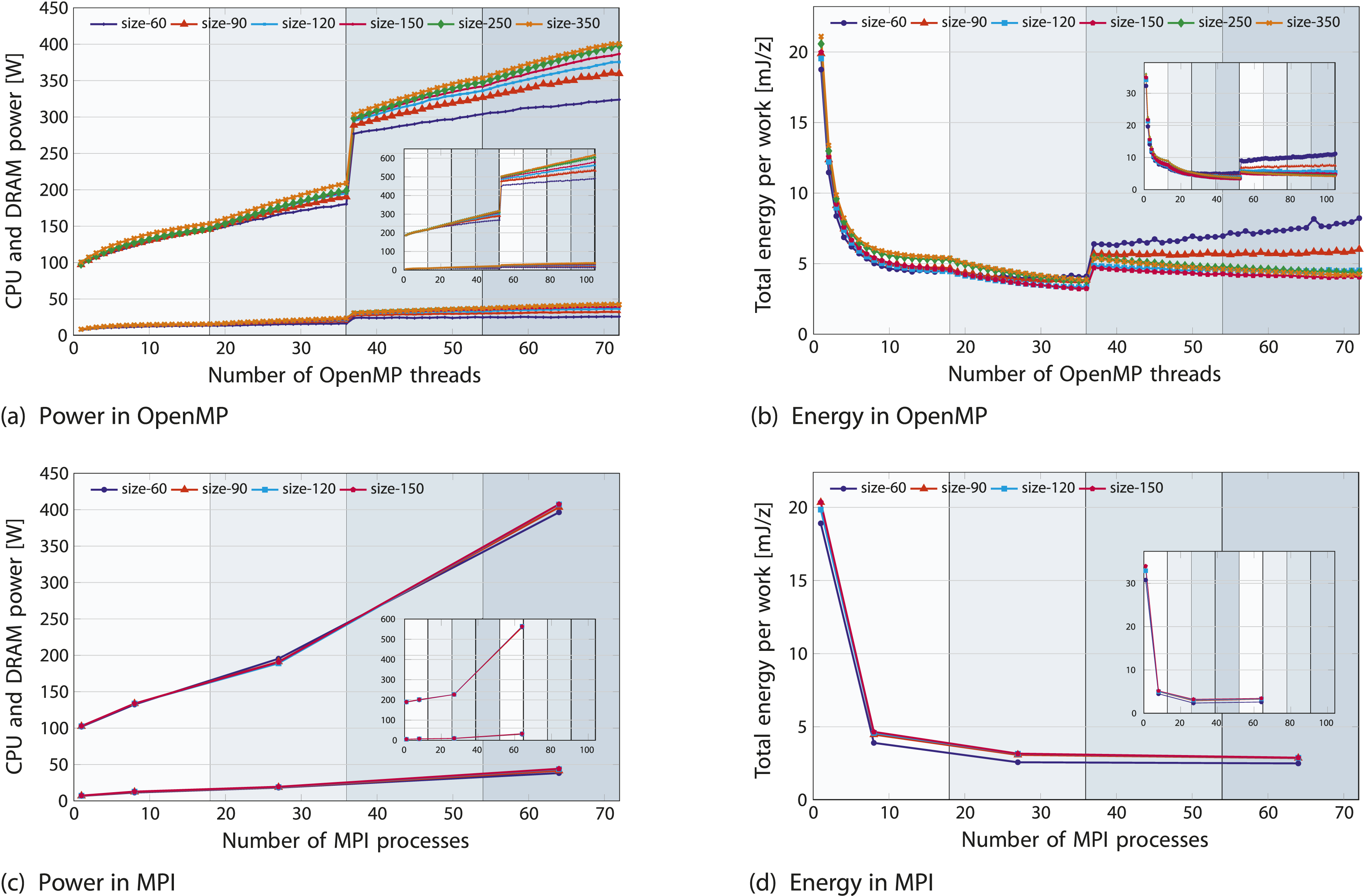

In Figure 5(b), beyond a single socket, as scaling declines sharply, the energy consumption on the second socket stays constant – showing no further decrease – with a noticeable shift at the switchover point. Given SPR’s higher peak performance and greater memory bandwidth compared to ICL, its performance scales proportionally, falling somewhere within the ratio of peak performance and memory bandwidth. For memory-bound codes, the theoretical increase of 40% (44.5% measured) in power consumption is offset by the 50% increase in memory bandwidth, resulting in comparable energy-to-solution on both systems but yielding lower EDP values on the SPR ccNUMA domain than Ice Lake. For example, energy consumption for the OpenMP implementation is 4.2 mJ/z on both the SPR node and the ICL node; see Figure 5(b).

Upshot: To isolate the impact of programming model choices from code implementation details, a comparison across different problem sizes shows that OpenMP overheads are more significant for smaller problem sizes. The general characteristics of the code are similar on both ICL and SPR architectures, while detailed performance and energy comparisons are specific to these chips.

6.2. Multi-node weak scaling

Figure 6(a) shows near-perfect weak scaling beyond a single node when scaling up to 31 ClusterA nodes or 22 ClusterB nodes (5³ to 13³ processes). The actual speedup closely aligns with the ideal speedup (based on a 5³ MPI process baseline), classifying LULESH as a scalable code. Within a node, memory bandwidth grows and the slight reduction in scaling is primarily caused by bandwidth sharing, as noted earlier. Figure 6(b) shows that with higher node counts, the per-node memory bandwidth remains nearly consistent for larger domains but gradually decreases for smaller domains. This deviation from the ideal horizontal line represents a loss in parallel efficiency. For example, for a 90³ domain size, bandwidth drops to 22% (ICL) and 11% (SPR).

Figure 6.

Weak scaling multi-node runs for the MPI-parallel LULESH application on the ICL-based ClusterA (subplot view in each plot: SPR-based ClusterB). The plots illustrate: (a) performance, (b) bandwidth, and (c) CPU power (top) and DRAM power (down) (d) energy, when scaling till 2197 processes (31 nodes of ClusterA and 22 nodes of ClusterB).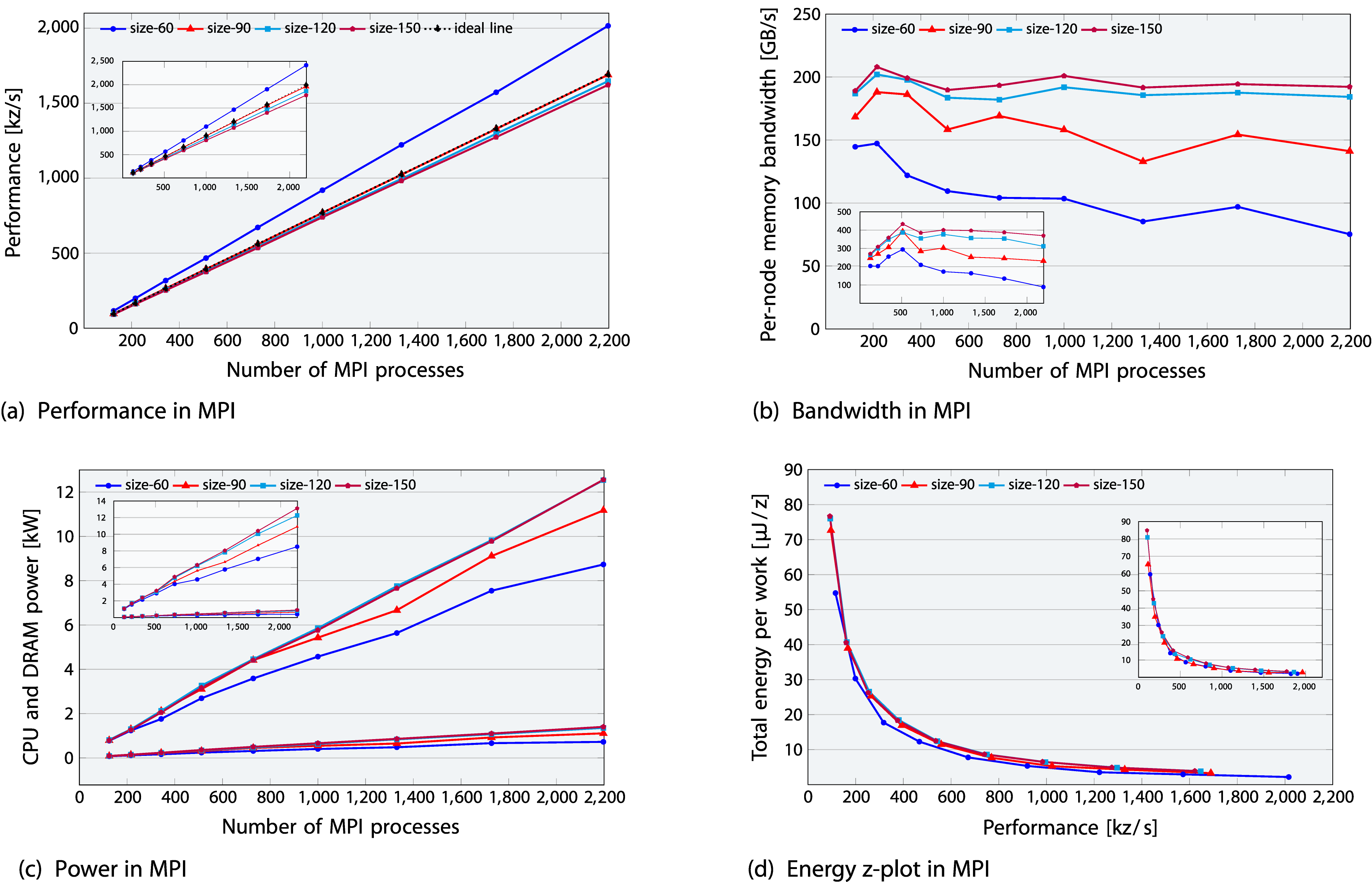

In Figure 6(c), on-chip power dissipation reaches 12.6 kW (81% of 15.5 kW TDP) for 31 ClusterA nodes and 13.1 kW (85% of 15.4 kW TDP) for 22 ClusterB nodes. To mitigate the trivial dependency of larger resources consuming more energy in week scaling, energy is normalized by the amount of work done. This is illustrated by plotting energy per work unit [J/z] on the y-axis and performance [z/s] on the x-axis while scaling resources for increasingly larger problems, as shown in Figure 6(d). The figure shows that good code scalability beyond the node level offsets the high power consumption of 81-85% of TDP, reducing the overall energy required per work unit. The inset subplot shows the same energy consumption but lower EDP for SPR-based ClusterB nodes compared to ICL-based ClusterA nodes, as expected. In contrast, the smaller 60³ domain size in blue, which fits into cache, presents an interesting case. It shows a more pronounced per-node memory bandwidth drop, reaching approximately 53% on ICL and 62% on SPR. However, as the cache effect reduces communication overhead, this leads to minimal energy to solution and EDP, resulting in both lower power dissipation and improved performance.

Upshot: Beyond a single node, LULESH shows nearperfect scaling and consistent per-node memory bandwidth for larger domains, offsetting high power consumption and yielding reduced energy to solution and EDP.

6.3. Vectorization impact

Performance was evaluated by progressively enabling vec- torization flags (-xSSE4.2, -xCORE-AVX2, -xCORE-AVX512) on the default scalar settings. The trivial trend that slower, non-vectorized LULESH code scales better than faster, vectorized code was observed. However, the performance gap was minimal, as only 6% of the vectorized code utilized AVX instructions. The contributions for scalar, 128-packed, 256-packed, 512-packed double instructions, as illustrated in Table 4, remain consistent across domain sizes and thread counts, except under MPI weak scaling.

Table 4.

Scalar and vectorized double instructions for code variants.

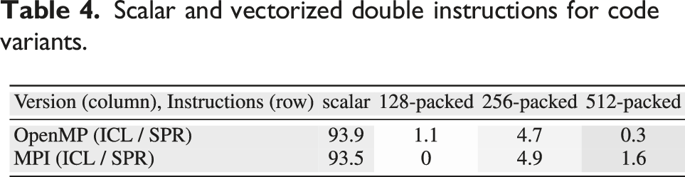
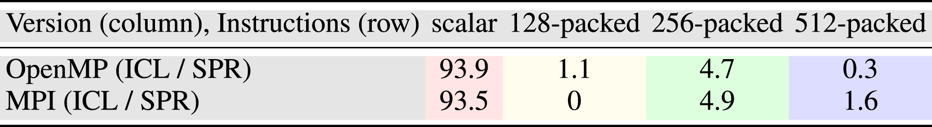
In the OpenMP variant, the sole non-memory-bound, non-vectorized function, calckinematicsForElems, presents optimization potential. In contrast, in the MPI variant, four of five non-memory-bound functions lack vec- torization and have potential for optimization, with only the UpdateVolumesForElems non-hot-spot function achieving 99.9% vectorized instructions. For example, the calckinematicsForElems hot spot accounts for about 13.2% (OMP-ICL), 14.3% (OMP-SPR), 14.9% (MPI-ICL) and 14.2% (MPI-SPR) of the overall execution time, suggesting that enhanced vectorization could boost performance by up to a factor of 4 to 8 (10% on the ccNUMA level). Similarly, the MPI hot spot IntegrateStressForElems, consuming 13.6% (MPI-ICL) and 12.5% (MPI- SPR) of execution time, offers similar optimization potential. In contrast, optimizing non-hot-spot functions like CalcCourantConstraintForElems, CalcHydroConstraintForElems, and UpdateVolumesForElems, which contribute only 0.8%, 0.3%, and 0.2% of total execution time, respectively, is unlikely to provide meaningful benefits.

Upshot: The performance gap between scalar and vectorized code (though minimal with only 6% AVX instructions) highlights optimization potential by vectorizing one OpenMP and two MPI non-memory-bound, non-vectorized hot spots.

6.4. Turbo mode impact

In Figure 7(a), results focus on the first chip, as data beyond it provides no new insights. On the second chip, the average frequency for all cores rises until saturation (69–72 cores), after which they stabilize at 3.08 GHz, dropping from 3.19 GHz. Measurements align with theoretical turbo tables of ICL and SPR obtained using likwid-powermeter. In SPR turbo mode, a similar trend is observed: 3.8 GHz in the first domain, dropping from 3.6 GHz to 3.0 GHz in the second. For brevity, only ICL results are shown, as SPR results do not differ qualitatively.

Figure 7.

Influence of turbo mode on memory bandwidth, performance, power and energy for the OpenMP-parallel LULESH application on ClusterA node. (a) The 3.48 GHz frequency of first domain decreases in the second domain. (b) The minimum, maximum and average statistics from 10 turbo mode runs are shown.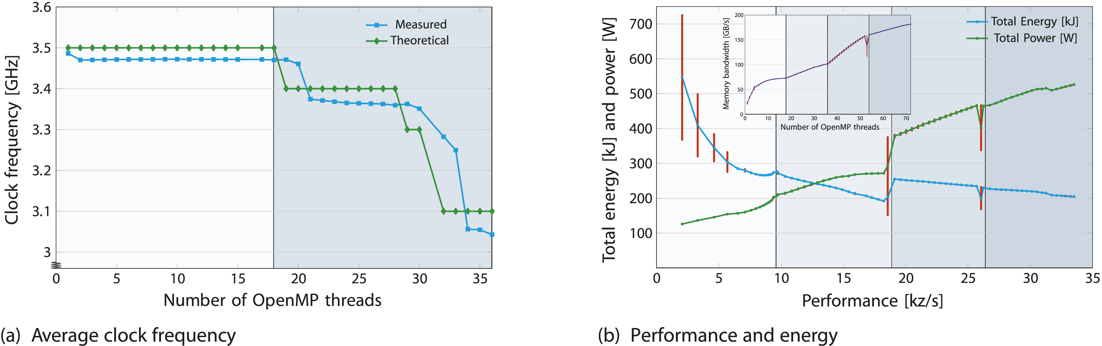

In Figure 7(b), warm-up steps were incorporated, and readings were repeated over 10 iterations, showing the maximum (top horizontal bars), minimum (bottom horizontal bars), and average (data points) statistics. An Ice Lake core in turbo mode reaches up to 3.5 GHz (46% above base frequency), and a node reaches 3.07 GHz (28% above base frequency), with a frequency boost occurring at chip switchover. Consequently, compared to the base frequency, turbo mode increases performance, memory bandwidth, on-chip power, and on-chip energy by approximately 6.7%, 7%, 22.8% (91.2% of the TDP), and 14.36%, respectively.

Upshot: Based on the Energy-Delay Product metric, turbo mode may not be the optimal choice, as the energy cost increases by approximately twice the performance gain.

6.5. Core frequency impact

Figure 8(a) suggests a linear relationship between total power W and CPU frequency f, expressed as

W = W_{0} + W_{d} f

(2)

Figure 8.

The influence of CPU clock frequency on the full LULESH application is presented for both (a), (b) OMP-ICL and (c) MPI-ICL variants. The second and third plots present a z-plot of total energy-to-solution versus performance, highlighting the optimal Energy Delay Product for various cores and core frequencies (1.0-2.8 GHz). The uncore frequency remains unfixed, ranging from a minimum of 0.8 GHz to a maximum of 2.5 GHz. The subplots in (b-c) display zoomed-in insets, while the subplot in (a) illustrates how the uncore frequency adjusts internally when the CPU frequency is fixed.

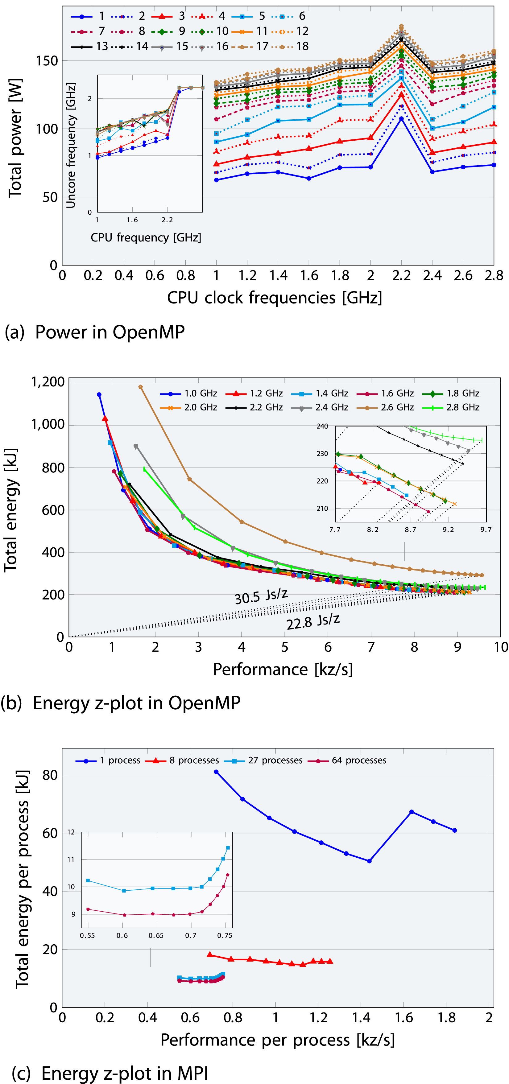
where the zero-frequency baseline power W₀ ranges from 40 to 120 W depending on the number of active cores, and W_d represents dynamic power. In contrast, the zero-core baseline power ranges from 55 to 95 W depending on the CPU clock frequency, out of which baseline DRAM power is limited to a narrow range of 3-5 W. These baseline (idle) powers were determined through linear regression for the CPU and curve fitting for DRAM, accounting for approximately 16%-48% of socket TDP and 19%-57% of socket total power. With the BIOS uncore frequency range set to 0.8–2.5 GHz and the performance-energy bias at 15 (lowest energy), uncore frequency adjusts dynamically when not explicitly set, as shown in the subplot inset of Figure 8(a). This causes a significant increase in power and energy consumption at a core frequency of 2.2 GHz, especially at lower core counts, as shown in Figure 8a–8(c). Since SPR findings are qualitatively similar and do not provide additional insights, we only present the ICL results for both OpenMP (Figure 8(a)-8(b)) and MPI variants (Figure 8(c)) for brevity.

In Figure 8(b), energy results for CPU frequencies below the base frequency are closely aligned, while CPU frequencies above the base frequency lead to higher energy consumption. For a single ccNUMA domain, the lowest CPU energy consumption occurs at 1.6 GHz, whereas 2.0 GHz achieves optimal energy efficiency (minimum EDP). This is because uncore frequencies are lower below 2.2 GHz and higher above it. If one is able to pay an additional energy, operating at 2.0 GHz frequency is optimal. However, if a power cap is required, this will be different, as lower CPU frequencies burn less power than 2.0 GHz.

In Figure 8(c), energy and performance are normalized by process count to isolate trivial weak-scaling effects, where more processes increase performance and energy use due to larger problem sizes. Similar to OpenMP results, exceeding a 2.0 GHz CPU frequency wastes energy with marginal performance gains, raising EDP. For example, increasing frequency from 2.0 GHz to 2.8 GHz with 64 processes (purple) yields only 5% more performance at a 15% energy cost.

Upshot: Adjusting the CPU clock frequency causes a 23% (5%) variation in performance and a 40% (15%) variation in energy consumption for OpenMP (MPI), highlighting the significant effect of core frequency on energy with 2.0 GHz identified as optimal. Though the impact remains relatively limited for lower frequencies.

6.6. Uncore frequency impact

Figure 9 presents results with uncore frequencies either left unset or fixed between 1.0 GHz and 2.2 GHz within a ccNUMA domain. As uncore frequency fixing is unavailable on ClusterA, the ICX36 node from another cluster was used, with uncore frequency configured via the likwid- setFrequencies tool. For brevity, we focus on the OMP-ICL variant, as other findings are similar. Figure 9(a) and 9(b) show that downclocking the uncore frequency reduces memory bandwidth by 29%, performance by 26%, and saves 42% power. This drop in memory bandwidth suggests it is not solely due to the lowered uncore frequency; rather, the LULESH code slows down as it comprises non-memory-bound functions (relying on L3 cache bandwidth influenced by uncore frequency) in addition to memory-bound functions. The performance reduction observed on the ICX36 node compared to the ClusterA node indicates that the uncore frequency, when left unset on ClusterA, operates at a significantly higher value, which enhances L3 cache speed and boosts performance. The ICX36 node operates slower due to its BIOS configuration, including an uncore frequency range of 1.0–2.2 GHz (vs. 0.8–2.5 GHz) and a performance-energy bias of 6 (middle of performance/energy scale) instead of 15 (lowest energy).

Figure 9.

Influence of uncore clock frequency on (a) performance (subplot view: bandwidth), (b) power versus cores (subplot view: power vs. uncore frequency) and (c) energy z-plot (subplot view: zoom-in) for the OpenMP-parallel LULESH application on a ccNUMA domain of an ICL domain. The core clock frequency is set to the base frequency of 2.4 GHz, while the uncore clock frequency is either left unset (min/max 2.4 GHz) or allowed to fix between 1.0 and 2.2 GHz.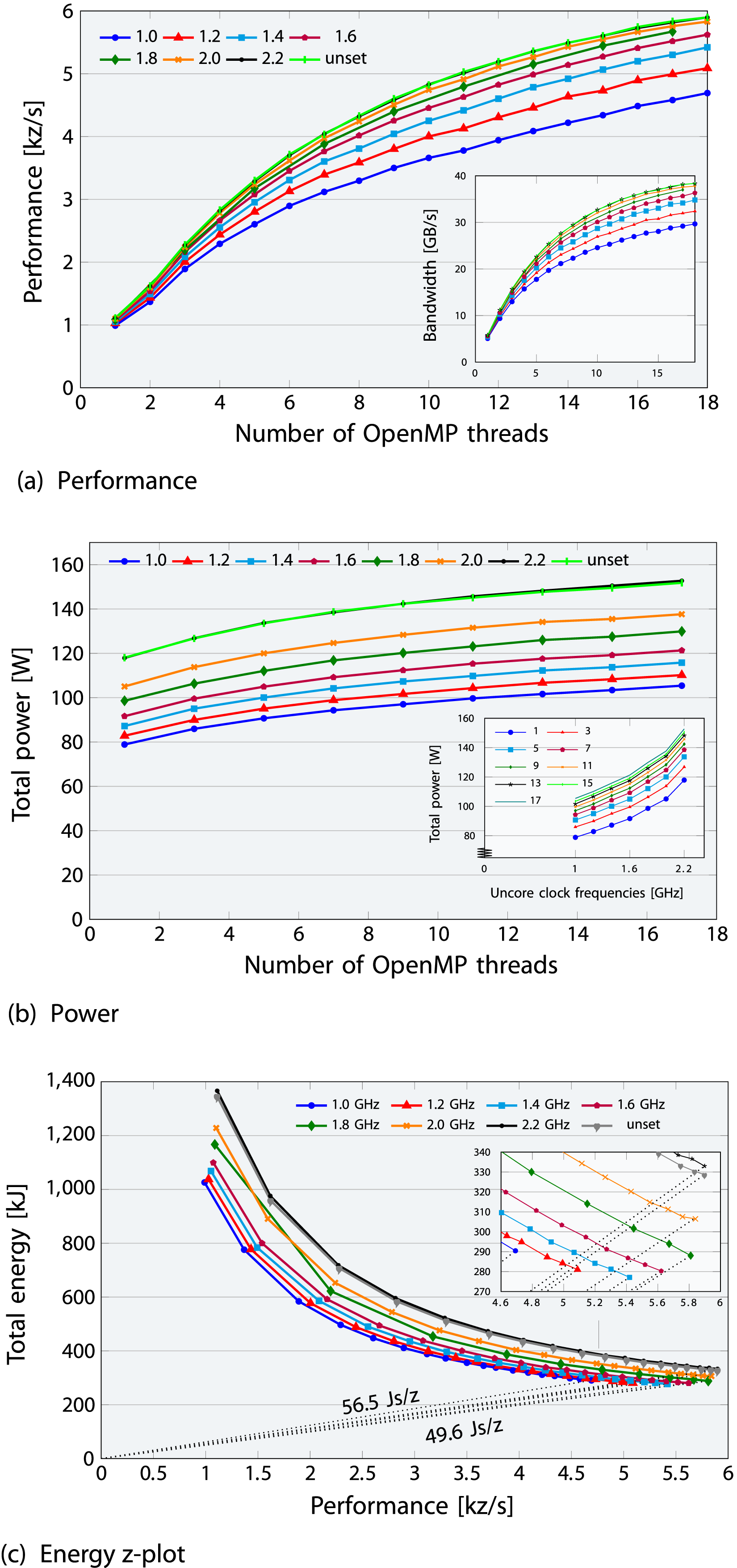

Figure 9(b) shows that the baseline power, ranging from 75 to 110 W (zero cores) to 65–90 W (zero frequency) across uncore clock frequencies with a fixed base CPU frequency on a ccNUMA domain, is more accurately represented by the zero-core value. The baseline (idle) power, accounting for 26–44% of the socket’s TDP, was estimated through linear regression by extrapolating to zero core or zero frequency. The subplot inset (for different core counts) shows that the linear frequency-power relationship holds up to 1.6 GHz. The observed non-linearity beyond this point is likely due to the CPU dynamically adjusting voltage with frequency to ensure proper chip operation, possibly as a preset for consistent regulation. At lower frequencies, the voltage decreases, but when the frequency drops to a level where voltage can no longer be reduced further, it remains constant, resulting in a linear power-frequency relationship. However, at higher frequencies above 1.6 GHz, voltage increases, leading to a non-linear trend. The noticeable increase in energy and power observed at CPU frequencies above 2.2 GHz, when the uncore frequency is unfixed on ClusterA (Figure 8) is an influence of varying uncore frequency, and thus vanishes in on-chip measurements with a fixed uncore frequency; however, this does not hold for DRAM measurements.

Figure 9(c) shows the global minimum energy-to-solution occurs at a uncore frequency of 1.4 GHz for the full ccNUMA domain (1 GHz for the single core), with only a 19% (34%) variation between the minimum and maximum. These variations from reducing the uncore frequency are lower than those in the previous Intel generation Hofmann et al. (2018). As a result, the entire domain (chip in general) should be used to minimize energy. Notably, in the highest 2.2 GHz uncore frequency scenario, a high baseline power drives the Energy-Delay Product to its peak. Increasing the uncore frequency boosts memory bandwidth until it saturates around 2.0 GHz. In the 1.6-1.8 GHz range of uncore frequency, there is still some leeway where memory bandwidth decreases less with decreasing uncore frequency, offering power savings and a minimum EDP.

Upshot: Adjusting the uncore clock frequency can result in a 26% variation in performance and a 20% variation in energy consumption, suggesting that fixing the uncore frequency has minimal impact, with 1.6-1.8 GHz being advisable.

7. Summary and future work

We presented an in-depth performance and energy analysis of the LULESH proxy application on two multi-core clusters with Intel Ice Lake (ICL) and Sapphire Rapids (SPR) processors, comparing OpenMP and MPI implementations. Each analysis section, both at the full application level and for individual kernels level, provides insights that collectively reveal LULESH’s performance and energy limitations, architectural impacts, and optimization potential.

Key takeaways In the kernel analysis, LULESH consists of six hot spot functions, whose runtime contribution is similar between the OpenMP and MPI implementations. However, four memory-bound functions in OpenMP exhibit scalable behavior in the MPI version, including one hot spot function, making them strong candidates for in-core optimizations rather than for memory data traffic reduction strategies. Compared to the full LULESH application within a single ccNUMA domain, all six hot spot functions converge within the same power range, consuming up to 58% of the total energy. Using the Roofline model, we provided performance limits for each memory-bound hot spot function. Using hardware performance counter events, we showed that actual measurements fall within the range between the best-case and worst-case predictions (achieved with write-allocate evasion and data reuse).

In the full application analysis for both ICL and SPR architectures, the code exhibits partly memory-bound characteristics, while the detailed comparison of energy and performance is specific to these architectures. To separate the impact of programming model choices from code implementation specifics, we compare the performance of OpenMP and MPI implementations across various problem sizes, noting that OpenMP implementation overheads become particularly significant for smaller problem sizes.

Hypothetical idle power consumption, defined as the extrapolated power consumption at zero active cores or zero frequency, is a critical factor for both CPUs compared to older Intel designs and is especially high on SPR, making concurrency throttling (using fewer cores for memory-bound code) less effective. A maximum of 40% variation in energy consumption was observed with core frequency adjustments and 20% with uncore frequency adjustments. Therefore, energy to solution can be reduced for LULESH by varying the number of cores, the core clock frequency, and the uncore clock frequency, although the impact of all of them is limited. For the performance-energy trade-off, LULESH exhibits a lower EDP on SPR than on ICL due to a complex interplay among SPR’s superior memory bandwidth, higher core count, higher power dissipation, and lower clock speed. While our results reflect the current performance and energy trade-offs on Intel CPUs, the metrics, analytical methods and insights employed are broadly applicable in similar high-performance applications.

Future work In future work, we aim to expand this analysis to hybrid parallelization strategies beyond pure MPI and pure OpenMP in order to further provide comprehensive insights into performance-energy trade-offs and optimization opportunities in LULESH and similar applications. Additionally, we anticipate interesting results from studying idle wave Afzal et al. (2019, 2021) and desynchronization Afzal et al. (2020, 2022) phenomena in LULESH, which exhibits a mix of memory- and compute- bound behavior. Our focus on Intel architectures was deliberate, allowing us to examine architectural evolution within a consistent platform. Expanding the study to include AMD and ARM CPUs, as well as GPU-based analyses using CUDA, would enhance generality. However, we have listed this as future work due to notable architectural differences. In particular, some kernels may exhibit different bottlenecks on these platforms, and GPU traffic analysis is further complicated by the non-deterministic execution order of thread blocks compared to CPUs. Although the HBM-enabled variant of Sapphire Rapids CPUs was not available at the time of this study, our methodology is directly applicable. We anticipate that the increased memory bandwidth would shift performance bottlenecks further toward the compute-bound regime. We will assess the performance of LULESH on architectures equipped with HBM or integrated accelerators or AI capabilities with traditional DRAM setups to clarify the benefits and potential synergies between computational and memory-bound tasks for LULESH and similar memory-intensive applications.

Supplemental Material

Supplemental Material - Analytic roofline modeling and energy analysis of the LULESH proxy application on multi-core clusters

Supplemental Material for Analytic roofline modeling and energy analysis of the LULESH proxy application on multi-core clusters by Ayesha Afzal, Georg Hager, Gerhard Wellein in The International Journal of High Performance Computing Applications.

Footnotes

Acknowledgements

The authors gratefully acknowledge the HPC resources provided by the Erlangen National High Performance Computing Center (NHR@FAU) of the Friedrich-Alexander-Universität Erlangen-Nürnberg (FAU). NHR funding is provided by the German Federal Ministry of Education and Research and the state governments participating on the basis of the resolutions of the GWK for the national high-performance computing at universities (). NHR@FAU hardware is partially funded by the German Research Foundation (DFG) – 440719683.

Funding

The author(s) disclosed receipt of the following financial support for the research, authorship, and/or publication of this article: This research is supported by a “Future Project” of the National High-Performance Computing at German universities (NHR), which focused on enhancing energy efficiency and managing operational costs across NHR centers.

Declaration of conflicting interests

The author(s) declared no potential conflicts of interest with respect to the research, authorship, and/or publication of this article.

ORCID iDs

Ayesha Afzal

Georg Hager

Supplemental Material

Supplemental material for this article is available online.

Notes

Author biographies

Ayesha Afzal holds a Master’s degree in Computational Engineering from Friedrich-Alexander-Universität Erlangen-Nürnberg, Germany, and a Bachelor’s degree in Electrical Engineering from the University of Engineering and Technology, Lahore, Pakistan. She is working toward the Ph.D. degree at the professorship for High Performance Computing at Erlangen National High Performance Computing Center (NHR@FAU), Germany. Her PhD research lies at the intersection of analytic performance models, performance tools and parallel simulation frameworks, with a focus on first-principles performance modeling of distributed-memory parallel programs.

Georg Hager holds a doctorate (Ph.D.) and a Habilitation degree in Computational Physics from the University of Greifswald, Germany. He leads the Research Division at Erlangen National High Performance Computing Center (NHR@FAU) and is an associate lecturer at the Institute of Physics at the University of Greifswald. Recent research includes architecture-specific optimization strategies for current microprocessors, performance engineering of scientific codes on chip and system levels, and the modeling of out-of-lockstep behavior in large-scale parallel codes.

Gerhard Wellein received the Diploma (M.Sc.) degree and a doctorate (Ph.D.) degree in Physics from the University of Bayreuth, Germany. He is a Professor at the Department of Computer Science at Friedrich-Alexander-Universität Erlangen-Nürnberg and heads the Erlangen National High Performance Computing Center (NHR@FAU). His research interests focus on performance modeling and performance engineering, architecture-specific code optimization, and hardware-efficient building blocks for sparse linear algebra and stencil solvers.

References

1.
Afzal A (2015) The cost of computation: metrics and models for modern multicore-based systems in scientific computing. Master’s Thesis, Department Informatik, Friedrich Alexander Universität Erlangen-Nürnberg.

2.
Afzal A Hager G Wellein G (2019) Propagation and decay of injected one-off delays on clusters: a case study. In: Proceedings of the 2019 IEEE International Conference on Cluster Computing. IEEE, 1–10.

3.
Afzal A Hager G Wellein G (2020) Desynchronization and wave pattern formation in MPI-parallel and hybrid memory-bound programs. In: Lecture Notes in Computer Science. Springer Science, Vol. 12151, 391–411.

4.
Afzal A Hager G Wellein G (2021) Analytic modeling of idle waves in parallel programs: communication, cluster topology, and noise impact. In: Lecture Notes in Computer Science. Springer Science, Vol. 12728, 351–371.

5.
Afzal A Hager G Wellein G (2022) The role of idle waves, desynchronization, and bottleneck evasion in the performance of parallel programs. IEEE Transactions on Parallel and Distributed Systems 34: 623–638, TPDS .

6.
Afzal A Hager G Wellein G (2023) SPEChpc 2021 benchmarks on Ice Lake and Sapphire Rapids infiniband clusters: a performance and energy case study. In: 14th IEEE/ACM Performance Modeling, Benchmarking and Simulation of High Performance Computer Systems (PMBS). IEEE.

7.
Afzal A Hager G Wellein G (2025) Analytic roofline modeling and energy analysis of the LULESH proxy application on multi-core clusters – performance data artifact appendix. DOI:10.5281/zenodo.14056331.

8.
Calore E Gabbana A Schifano SF , et al. (2020) ThunderX2 performance and energy-efficiency for HPC workloads. Computation 8(1): 20. doi: 10.3390/computation8010020. Available at: https://doi.org/10.3390/computation8010020

9.
Carothers CD Meredith JS Blanco MP , et al. (2017) Durango: scalable synthetic workload generation for extreme-scale application performance modeling and simulation. In: Proceedings of the 2017 ACM SIGSIM Conference on Principles of Advanced Discrete Simulation, Singapore, May 24th-26th, 97–108. DOI: 10.1145/3064911.3064923.

10.
Chishti MA Khan S Mustafa Z , et al. (2020) Energy-efficient HPC: LULESH on Arm-based clusters. 2020 International Conference on High Performance Computing (HiPC). IEEE, 1–10. Available at: https://doi.org/10.1109/HiPC51435.2020.00014

11.
Copik M Calotoiu A Grosser T , et al. (2021) Extracting clean performance models from tainted programs. In: Proceedings of the 26th ACM SIGPLAN Symposium on Principles and Practice of Parallel Programming, PPoPP ’21. New York, NY, USA: Association for Computing Machinery, 403–417. DOI: 10.1145/3437801.3441613.

12.
Hofmann J Hager G Fey D (2018) On the accuracy and usefulness of analytic energy models for contemporary multicore processors. In: Yokota R Weiland M Keyes D , et al. (eds) High Performance Computing. Cham: Springer International Publishing, 22–43. DOI: 10.1007/978-3-319-92040-52.

13.
Ibrahim M Hassan A Al-Kiswany S , et al. (2021) Exploring heterogeneous CPU-GPU-FPGA architectures for energy-efficient scientific workloads. Journal of Parallel and Distributed Computing 150: 120–135. doi: 10.1016/j.jpdc.2021.03.009. Available at: https://doi.org/10.1016/j.jpdc.2021.03.009

14.
Jin Z Finkel H (2019) Evaluating LULESH kernels on OpenCL FPGA. In: Kumari P Amaral JN Revuelto P (eds). Applied Reconfigurable Computing. ARC 2019, Lecture Notes in Computer Science. Cham: Springer, 11404, 151–163. Available at: https://doi.org/10.1007/978-3-030-17227-515

15.
Karlin I Keasler J Neely R (2012) LULESH 2.0 Updates and Changes. Technical Report. Lawrence Livermore National Laboratory. https://asc.llnl.gov/sites/asc/files/2023-05/LULESH2.0_Changes.pdf

16.
Karlin I Bhatele A Keasler J , et al. (2013) Exploring traditional and emerging parallel programming models using a proxy application. In: 2013 IEEE 27th International Symposium on Parallel and Distributed Processing. IEEE, 919–932. DOI: 10.1109/IPDPS.2013.115.

17.
León EA Karlin I Grant RE (2015) Optimizing explicit hydrodynamics for power, energy, and performance. 2015 IEEE International Conference on Cluster Computing. IEEE, 11–21. Available at: https://doi.org/10.1109/CLUSTER.2015.12

18.
León EA Karlin I Grant RE , et al. (2016b) Program optimizations: the interplay between power, performance, and energy. Parallel Computing 58: 56–75.

19.
León EA Karlin I Moody AT (2016a) System noise revisited: enabling application scalability and reproducibility with SMT. In: 2016 IEEE International Parallel and Distributed Processing Symposium (IPDPS). IEEE, 596–607. DOI: 10.1109/IPDPS.2016.48.

20.
Liu C Kulkarni M (2015) Optimizing the LULESH stencil code using concurrent collections. In: Proceedings of the 5th International Workshop on Domain-specific Languages and High-Level Frameworks for High Performance Computing. New York, NY, USA: Association for Computing Machinery. DOI: 10.1145/2830018.2830024.

21.
Malony AD Larsen M Huck K , et al. (2020) When parallel performance measurement and analysis meets in situ analytics and visualization. In: Parallel Computing: Technology Trends. IOS Press, 521–530. DOI: 10.3233/APC200080.

22.
Marques D Duarte H Ilic A , et al. (2017) Performance analysis with cache-aware roofline model in intel advisor. In: 2017 International Conference on High Performance Computing & Simulation (HPCS), Genoa, Italy, July 17-21, 2017, 898–907. DOI: 10.1109/HPCS.2017.150.

23.
Singanaboina SY Wei W Tsaousis Seiras I , et al. (2024) Accelerating LULESH using HPX - the C++ standard library for parallelism and concurrency. Practice and Experience in Advanced Research Computing 2024: Human Powered Computing. New York, NY, USA: Association for Computing Machinery. Available at: https://doi.org/10.1145/3626203.3670529

24.
Stratton JA Calkins J Trott CR , et al. (2013) Kokkos performance portability for LULESH on GPU architectures. Proceedings of the International Conference on High Performance Computing, Networking, Storage and Analysis (SC ’13). New York, NY, USA: ACM, 1–11. Available at: https://doi.org/10.1145/2491266.2491276

25.
Treibig J Hager G Wellein G (2010) LIKWID: a lightweight performance-oriented tool suite for x86 multicore environments. In: 2012 41st International Conference on Parallel Processing Workshops, 207–216. IEEE. DOI: 10.1109/ICPPW.2010.38.

26.
Williams S Waterman A Patterson D (2009) Roofline: an insightful visual performance model for multicore architectures. Communications of the ACM 52(4): 65–76. DOI: 10.1145/1498785.

27.
Williams S Waterman A Patterson D (2010) Scientific computing with GPUs: performance and energy efficiency. Proceedings of the 2010 ACM/IEEE International Conference for High Performance Computing, Networking, Storage and Analysis (SC ’10). Washington, DC, USA: IEEE Computer Society, 1–11. Available at: https://doi.org/10.1145/1870578.1870657

28.
Wittmann M Hager G Zeiser T , et al. (2016) Chip-level and multi-node analysis of energy-optimized lattice Boltzmann CFD simulations. Concurrency and Computation: Practice and Experience 28(7): 2295–2315.

29.
Wu X Taylor V Cook J , et al. (2017) Performance and power characteristics and optimizations of hybrid MPI/OpenMP LULESH miniapps under various workloads. Proceedings of the 5th International Workshop on Energy Efficient Supercomputing, E2SC’17. New York, NY, USA: Association for Computing Machinery.

Supplementary Material

Please find the following supplemental material available below.

For Open Access articles published under a Creative Commons License, all supplemental material carries the same license as the article it is associated with.

For non-Open Access articles published, all supplemental material carries a non-exclusive license, and permission requests for re-use of supplemental material or any part of supplemental material shall be sent directly to the copyright owner as specified in the copyright notice associated with the article.

0.00 MB

0.66 MB