Sage Journals: Discover world-class research

Abstract

Large-scale multiphysics simulations are computationally challenging due to the coupling of multiple processes with widely disparate time scales. The advent of exascale computing systems exacerbates these challenges since these systems enable ever-increasing size and complexity. In recent years, there has been renewed interest in developing multirate methods as a means to handle the large range of time scales, as these methods may afford greater accuracy and efficiency than more traditional approaches of using implicit-explicit (IMEX) and low-order operator splitting schemes. However, to date there have been few performance studies that compare different classes of multirate integrators on complex application problems. In this work, we study the performance of several newly developed multirate infinitesimal (MRI) methods, implemented in the SUNDIALS solver package, on two reacting flow model problems built on structured mesh frameworks. The first model revisits prior work on a compressible reacting flow problem with complex chemistry that is implemented using BoxLib but where we now include comparisons between a new explicit MRI scheme with the multirate spectral deferred correction (SDC) methods in the original paper. The second problem uses the same complex chemistry as the first problem, combined with a simplified flow model, but runs at a large spatial scale where explicit methods become infeasible due to stability constraints. Two recently developed IMEX MRI multirate methods are tested. These methods rely on advanced features of the AMReX framework on which the model is built, such as multilevel grids and multilevel preconditioners. The results from these two problems show that MRI multirate methods can offer significant performance benefits on complex multiphysics application problems and that these methods may be combined with advanced spatial discretization to compound the advantages of both.

Keywords

multirate integration multirate infinitesimal schemes spectral deferred corrections structured grids combustion

1. Introduction

The advent of exascale computing will allow modeling of far larger and more complex systems than ever before. In taking advantage of these systems, scientific simulations in areas such as climate, combustion, astrophysics, and fusion sciences are adding increasingly complex physical models with processes often evolving on widely varying time scales and requiring tighter, more accurate coupling. For example, in atmospheric climate modeling, cloud microphysics, gas dynamics, and ocean currents each evolve at different rates. In combustion, even for modest reaction mechanisms, the difference in time scales between stiff chemical kinetics, species/thermal diffusion, and acoustic wave propagation can easily span two or more orders of magnitude; convective time scales can be an additional one or two orders of magnitude slower.

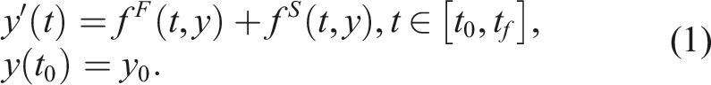
Motivated by these large-scale multiphysics, multirate simulations composed of coupled models for interacting physical processes, we consider ordinary differential equation (ODE) initial value problems (IVPs) containing two time scales:

\begin{array}{l} y^{'} (t) = f^{F} (t, y) + f^{S} (t, y), t \in [t_{0}, t_{f}], \\ y (t_{0}) = y_{0} . \end{array}

(1)

Here t is time, the dependent variable is

y \in R^{N}

, y′ denotes dy/dt,

f^{F} : R \times R^{N} \to R^{N}

and

f^{S} : R \times R^{N} \to R^{N}

are partitions of the operator that advance at fast and slow timescales, respectively, and

y_{0} \in R^{N}

is the initial state evolved from time t₀ to t_f. For such problems, single-rate implicit time integration methods can become prohibitively expensive due to the cost and complexity of large, monolithic algebraic solvers. Similarly, single-rate explicit integration methods may become infeasible due to stability constraints arising from the fastest process in the system. Thus, practitioners frequently evolve the fast portion using small time steps, h, and the slow portion with a larger time step, H ≫ h. In many multiphysics circumstances, even these slow processes are frequently decomposed further into those for which explicit time-stepping methods provide sufficient accuracy and efficiency and those for which implicit methods are preferred to overcome restrictive stability limitations on the time step size for explicit approaches. Such combinations are often treated using a mixed implicit-explicit (IMEX) scheme. Thus, in this work, we also consider the additional splitting of the problem into three components:

\begin{array}{l} y^{'} (t) = f^{F} (t, y) + f^{I} (t, y) + f^{E} (t, y), t \in [t_{0}, t_{f}], \\ y (t_{0}) = y_{0} . \end{array}

(2)

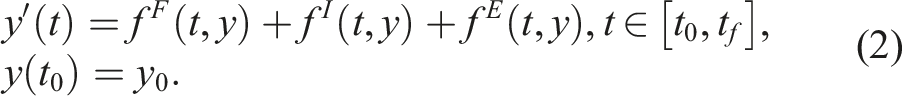
This may be achieved by splitting f^S from equation (1) into f^I + f^E, where the slow, non-stiff terms are grouped into f^E and evolved using explicit methods, while the slow, stiff terms are grouped into f^I and evolved using implicit methods. Returning to the combustion example above, one could apply either of the multirate splittings of equation (1) or equation (2), placing the stiff chemical kinetics in the operator f^F and the remainder in f^S, or further partitioning the species/thermal diffusion into f^I and acoustic wave propagation into f^E.

Traditional multirate approaches based on operator splitting have been used for many years for both equation (1) and equation (2) with varying degrees of success, but these approaches have historically been limited to second-order. In recent years, new multirate methods have been developed to allow for high-order integration algorithms that advance each partition at its own timescale potentially with a method tailored to each process. These state-of-the-art multiphysics coupling schemes can further accelerate the discovery process by allowing even more efficient use of supercomputing resources.

In large-scale simulation, the efficiency of the spatial discretization matters greatly as well. A wide range of approaches for the spatial discretization of partial differential equations (PDEs) are based on structured grids. Structured grid frameworks have a number of desirable properties in general and are increasingly favorable when leveraging exascale computing systems. Due to their regular grid structures, they offer a high degree of control over domain decomposition and parallel distribution of grids as well as low memory overhead due to simpler connectivity. There is a rich history of numerical methods for structured grids that offer regular stencils and desirable data locality properties. Regular stencils lead to efficient vectorization on manycore/GPU architectures, and improved data locality leads to fewer cache misses. Block-structured adaptive mesh refinement (AMR) is a widely used strategy within the structured grid community that focuses computational power in regions of interest while retaining complete control over the grid structure. There are numerous applications and numerical methods that can take advantage of such a strategy in the fields of fluid mechanics, combustion, astrophysics, electromagnetism, and cosmology (Almgren et al., 2013; Day and Bell, 2000; Fan et al., 2019; Sexton et al., 2021; Vay et al., 2018), just to name a few.

In addition to novel algorithms, newly developed numerical software targeted at efficient utilization of next-generation supercomputing architectures is becoming increasingly available. These packages are often open source, developed for portability, and can provide highly performant numerical methods within a structure that allows for continued development and extension of capabilities. Both the United States Department of Energy and the European Union have made considerable investments in such software, and many scientific applications employ them on high-performance systems. In addition, the Extreme-scale Software Development Kit (xSDK) has developed community policies and standards that encourage such packages to adopt interoperability on many levels, both strengthening the capabilities available as well as their usability within complex scientific application codes (Bartlett et al., 2017).

The goal of this paper is to understand the relative potential benefits of high-order multirate time integration schemes posed on adaptive, structured meshes. Both the multirate methods and the structured AMR algorithms are instantiated within numerical software packages contained within the xSDK. We consider reactive flow problems because they exhibit properties common to many multiphysics systems. In particular, they include both fast (chemistry reaction systems) and slow (diffusion, acoustic, and/or convective) time dynamics and require a mixture of time integration methods for optimal performance. A recent development in reactive flow simulation is the use of spectral deferred corrections (SDC) as a multirate temporal integrator. High-order multirate infinitesimal (MRI) approaches developed over the last decade also offer potential speedups and robust alternatives to SDC on these problems.

There have been few performance studies for multirate integration on complex application problems. Here, we compare several MRI schemes supported by the ARKODE package (Reynolds et al., 2023) in the SUNDIALS library (Gardner et al., 2022; Hindmarsh et al., 2005) of time integrators and nonlinear solvers to an existing SDC implementation for a combustion problem containing detailed kinetics and transport using the BoxLib block-structured AMR framework (Zhang et al., 2016). Additionally, we look at the performance of newly developed explicit and implicit-explicit (IMEX) multirate methods on a similar problem implemented with the AMReX block-structured AMR framework (Zhang et al., 2019, 2021). BoxLib is the predecessor to AMReX, contains a subset of features offered in AMReX (such as grid generation and MPI communication), and includes a complete SDC implementation of the combustion problem in our comparisons. AMReX is a software framework developed by the Exascale Computing Project (ECP) Block Structured Adaptive Mesh Refinement Co-Design Center and is designed to support structured adaptive grid calculations on massively parallel manycore/GPU machines. Also as part of the ECP, SUNDIALS has recently added several additional capabilities for integrating problems on GPU-based systems (Balos et al., 2021). This work compares the performance of multirate methods for combustion using SDC and integrators available within the SUNDIALS time integrator library. Our numerical experiments are performed using the AMReX and BoxLib frameworks.

The rest of the paper is organized as follows. The next section overviews the multirate and SDC time integration approaches and specific methods of interest to this work. Section 3 presents the mathematical formulation of the combustion problems we use to evaluate the performance of the integration methods. In Section 4, we provide overviews of AMReX and SUNDIALS and describe how we implemented our models in the combined SUNDIALS-AMReX framework. In the next sections, we present results on two reacting flow problems. Section 5 examines various explicit multirate schemes using a detailed combustion model, and Section 6 presents results from an AMReX implementation of various IMEX multirate schemes for a modified reacting flow model. Section 7 summarizes the work and our findings. Finally, Section 8 lists acronyms used throughout the text, along with their meanings and references for further detail.

2. Multirate time integration

Many applications handle the varying time scales found in multiphysics systems using multirate approaches, where smaller time steps are used for rapidly evolving operators and larger steps are used for more slowly evolving components. A popular, long-used approach to many multiphysics problems is use of low-order operator splitting with subcycling, e.g., first-order Lie–Trotter splitting (McLachlan and Quispel, 2002) or second-order Strang–Marchuk splitting (Marchuk, 1968; Strang 1968). However, these methods can suffer from a lack of stability and accuracy (Estep et al., 2008; Knoll et al., 2003). Higher order splitting methods have been developed, but they often require backward time integration (Cervi and Spiteri, 2019; Goldman and Kaper, 1996), which increases both the run time cost as well as the development time for code infrastructure.

Another highly flexible approach that multiphysics applications have used to handle multiple time scales is the use of SDC methods (Dutt et al., 2000). In these methods, a series of correction equations are integrated to reduce error at each iteration in the series. Typically, a low-order method is used to integrate the system at each iteration, and these solutions are applied iteratively to build schemes of arbitrarily high accuracy. The methods have been extended to handle solutions of multirate partial differential equation systems allowing for custom methods to be applied for each specific time scale and/or operator (Bourlioux et al., 2003; Layton and Minion, 2004). While the SDC methods provide considerable freedom in the schemes used to integrate each scale and operator, they do require an integration over each point in time for each iteration, generally resulting in several passes over the time domain to generate a high-order solution. However, SDC methods have been used in the multiphysics community for some time (Huang et al., 2020; Nonaka et al., 2012; Pazner et al., 2016; Zingale et al., 2019) because of their relative ease in implementation by adapting established operator splitting implementations. Specifically, high-order multirate approaches based on SDC have been shown to be effective on combustion problems with complex chemistry (Emmett et al., 2014, 2019). Within the combustion community, the long-time standard has been to employ high-order, explicit Runge–Kutta approaches such as those used in the S3D code (Chen et al., 2009). In Emmett et al. (2014), a multirate SDC approach for combustion was introduced in the “SMC” code, and a direct comparison between SMC and S3D demonstrated that integration in SMC can offer at least a 4x speedup over the widely used fourth-order explicit Runge–Kutta method for moderately-sized chemical mechanisms.

In the meantime, novel classes of multirate methods that show strong potential for a more efficient approach to high temporal order have been developed. Starting with Gear and Wells (1984) and continuing with Sand and Skelboe (1992); Günther and Sandu (2016); Roberts et al. (2021); and Luan et al. (2020), multirate time integration methods were developed to address efficiency and accuracy issues associated with operator splitting approaches. One particular multirate method, the multirate infinitesimal generalized additive Runge–Kutta (MRI-GARK) method (Sandu, 2019), has some distinct advantages over other multirate methods. These schemes are a recent addition to the broader class of infinitesimal methods, including the multirate infinitesimal step (MIS) methods (Schlegel, 2011; Schlegel et al., 2009), that pioneered the approach. Both MIS and MRI methods integrate a multirate problem in the form of equation (1) for one slow time step by alternating between evaluations of f^S and advancing with f^F for several fast steps. With methods of this form, no part of the time step is repeated, and the method used for integrating the fast partition is left unspecified, allowing for specialized schemes tailored to the fast operator. Thus, MRI- and MIS-based methods allow extreme flexibility regarding methods applied to problem components, while simultaneously enabling high accuracy, without the requirement for backward-in-time integration or repeated evaluation of the step.

In the following subsections, we provide more detail about the specific classes of MRI and SDC approaches used in this work.

2.1. IMEX-MRI-GARK

The first class of multirate schemes that we consider is the implicit-explicit multirate infinitesimal GARK (IMEX-MRI-GARK) methods from Chinomona and Reynolds (2021). These schemes are a recent addition to the broader class of infinitesimal methods that generalize the previously-mentioned MIS and MRI-GARK methods constructed for problems of the form equation (1). Methods within this family share two fundamental traits. First, they utilize a Runge–Kutta-like structure for each time step t_n → t_n + H, wherein the overall time step is achieved through computation of s internal stages that are eventually combined to form the overall time step solution y_n+1 ≈ y (t_n + H). These internal stages roughly correspond to approximations Y_i ≈ y (t_n + c_iH), i = 1, …, s, where a specific scheme includes an array of coefficients $c \in R^{s}$ that define these stage times. Second, these methods couple the fast and slow time scales by solving a set of modified fast IVPs to obtain the internal stages. Specifically, to compute the updated solution y_n+1 from y_n, these methods perform the algorithm:

1. Set Y₁ = y_n and T₁ = t_n.

2. For i = 2, …, s:

a. Let v (T_i−1) = Y_i−1, T_i = t_n + c_iH, and Δc_i = c_i − c_i−1 and define a “forcing” polynomial r_i(θ) constructed from evaluations of f^S (T_j, Y_j) where j = 1, …, i.

b. Solve the “fast” IVP over θ ∈ [T_i−1, T_i]:

v^{'} (θ) = f^{F} (θ, v (θ)) + r_{i} (θ) .

(3)

c. Set Y_i = v (T_i).

3. Set y_n+1 = Y_s.

When r_i(θ) depends on f^S(T_i, Y_i), step 2b is implicit in Y_i; however, when Δc_i = 0, that step simplifies to a standard Runge–Kutta update. Thus, infinitesimal methods that allow implicit treatment of f^S typically only allow implicit dependence on Y_i for stages where Δc_i = 0, resulting in a “solve-decoupled” approach. Here, the stages alternate between a standard diagonally-implicit slow nonlinear system solve and evolving the modified fast IVP. We note that since step 2b may be solved using any sufficiently accurate algorithm, these methods offer extreme flexibility for practitioners to employ problem-specific integrators. A schematic of the structure is shown in Figure 1(b).

Figure 1.

Comparison of the structure of MRSDC and MRI methods. (a) Schematic of MRSDC-332 using the 3-point Gauss–Lobatto quadrature for the coarse nodes and applying a 3-point Gauss–Lobatto quadrature two times within each coarse subinterval. The horizontal arrows demarcate the subintervals within the coarse interval. The vertical arrows indicate the flow of information between iterations. (b) Schematic of an MRI-IMEX method. The loops indicate where stages with Δc_i = 0 are inserted for “solve-decoupled” implicit stepping. Arrows denote the flow of information between stages.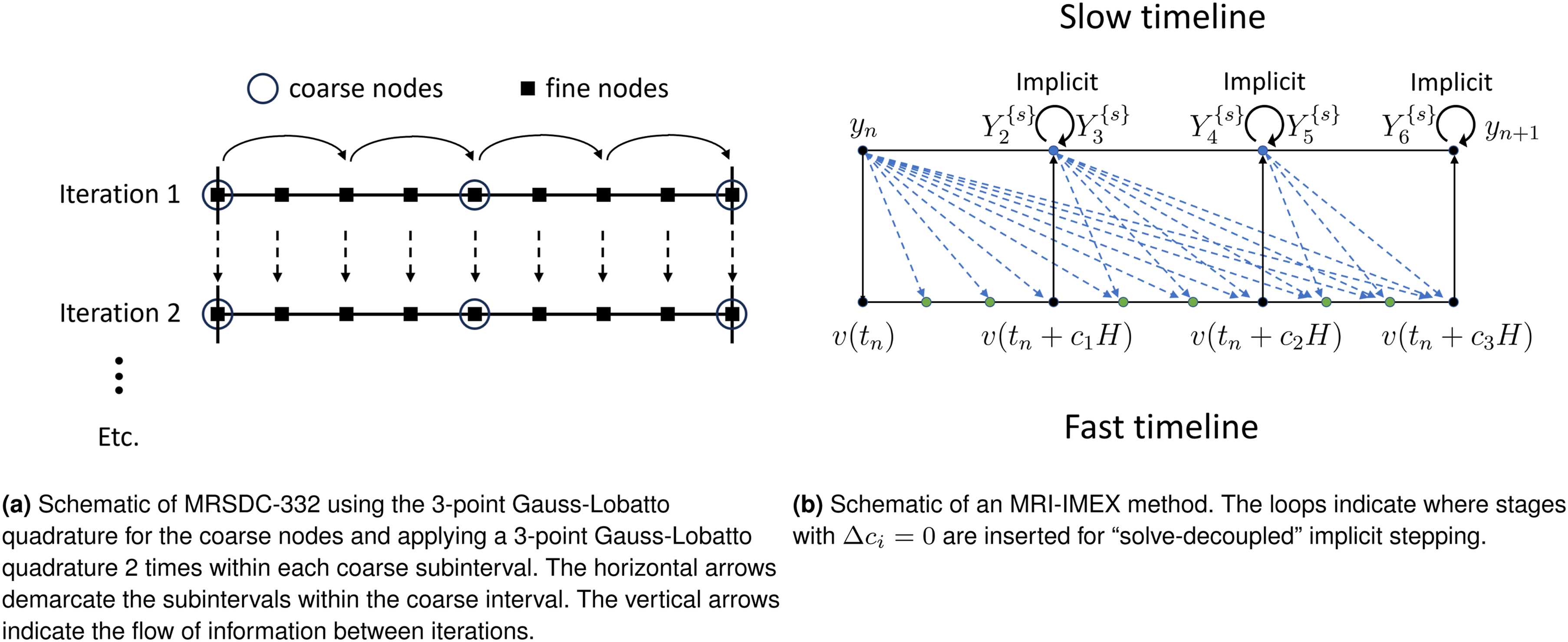

Within this infinitesimal family, the MIS methods first introduced by Schlegel et al. (2009) and Schlegel (2011) treat the slow time scale operator f^S explicitly and result in up to $O (H^{3})$ accuracy. The MRI-GARK methods introduced by Sandu (2019) treat f^S using either an explicit or a solve-decoupled implicit scheme and result in up to $O (H^{4})$ accuracy. The IMEX-MRI-GARK methods proposed by Chinomona and Reynolds (2021) treat the slow time scale using ImEx methods, f^S = f^I + f^E, and result in up to $O (H^{4})$ accuracy. Additionally, within IMEX-MRI-GARK methods, either of the components, f^I or f^E, may be zero, resulting in an MRI-GARK method.

We note that these flexible infinitesimal formulations are not new, as the longstanding Lie–Trotter and Strang–Marchuk operator splitting methods similarly allow arbitrary algorithms at the fast time scale, as well as explicit, implicit, or IMEX treatment of the slow time scale. However, both of these approaches use the forcing function r_i(θ) = 0, resulting in $O (H)$ and $O (H^{2})$ accuracy, respectively.

2.2. Multirate SDC methods

Spectral deferred correction algorithms are a class of numerical methods that represent the solution as an integral in time and iteratively solve a series of correction equations designed to reduce the error. The SDC approach was introduced in Dutt et al. (2000) for the solution of ordinary differential equations. The correction equations are typically formed using a first-order time-integration scheme but are applied iteratively to construct schemes of arbitrarily high accuracy. In practice, the time step is divided into subintervals, and the solution at the end of each subinterval is iteratively updated using (typically) forward or backward Euler temporal discretizations. Each set of correction sweeps over all the subintervals increases the overall order of the method by one, up to the underlying order of the numerical quadrature rule over the subintervals. Thus, it is advantageous to define the subintervals using high-order numerical quadrature rules, such as Gauss-Lobatto, Gauss-Radau, Gauss-Legendre, or Clenshaw-Curtis.

There have been a number of works that have extended the SDC approach to handle physical systems with multiple disparate time scales. Minion (2003) introduces a semi-implicit version for ODEs with stiff and non-stiff processes, such as advection–diffusion systems. The correction equations for the non-stiff terms are discretized explicitly, whereas the stiff term corrections are treated implicitly. Bourlioux et al. (2003) introduce a multirate SDC (MRSDC) approach for PDEs with advection-diffusion-reaction processes where advection terms are evaluated explicitly, reaction and diffusion terms are treated implicitly, and different time steps are used for each process. For example, the “slow” advection process can be discretized using Gauss–Lobatto quadrature over the entire time step, while the stiffer diffusion/reaction processes can be subdivided into Gauss–Lobatto quadrature(s) within each of the advection nodes. This approach was also used successfully by Layton and Minion (2004) for a conservative formulation of reacting compressible gas dynamics. More recently, approaches have been developed for fourth-order, finite volume, adaptive mesh simulations (Emmett et al., 2019), as well as eighth-order finite differences (Emmett et al., 2014). The latter paper, known as the “SMC” algorithm, forms the basis of the comparisons in this paper to the aforementioned MRI integrators.

Multirate SDC offers flexibility in (i) the number of physical processes and how they are grouped together, (ii) the choices of intermediate quadrature points each process uses, and (iii) the form of the correction equation for each process. A long review can be found in the references above and mentioned within. Here, we will describe one particular approach taken in the SMC algorithm that forms the basis of our comparisons that follow.

For the MRSDC methods in this paper, we consider Gauss–Lobatto quadrature, noting that both endpoints of any given interval are included in the quadrature. We divide the overall time step into a series of coarse substeps using nodes at time t_p, and each coarse substep is further divided into a series of finer substeps using nodes at time t_q. With this choice of quadrature, each coarse node at time t_p corresponds to a location where a fine node also exists. For comparison against the MRI schemes in this paper, we group advection and diffusion together as a “slow” explicit process, f^S, and evaluate these on the coarse nodes. We treat reactions as the “fast” explicit process, f^F, and evaluate their terms on fine nodes. Other configurations are possible, e.g., mixed implicit-explicit methods for the slow time scale with diffusion treated implicitly in f^I (Bourlioux et al., 2003). To describe the temporal scheme, we use the terminology “MRSDC-XYZ”, where X is the number of coarse nodes, and we apply a Y-node quadrature Z times in each coarse subinterval. As an example, Figure 1(a) shows a graphical illustration of an MRSDC-332 scheme with the 3-point Gauss–Lobatto quadrature, which consists of 3 equally-spaced points. Note that, in general, there are n_q = X + (X − 1)(Z − 1) + (X − 1)(Y − 2)Z total fine nodes.

The MRSDC scheme begins by supplying an initial guess for the solution at all nodes at time t_q (typically the solution at t_n is used), denoted $y_{q}^{k}$ , where k is the iteration index. Each MRSDC iteration consists of a sweep over all the fine nodes at time t_q in order, updating the solution from $y_{q}^{k}$ to $y_{q}^{k + 1}$ . Each iteration in k increases the overall order of accuracy by one (when using forward or backward Euler), up to the order of accuracy of the underlying quadrature. When all processes are treated explicitly, the forward-Euler correction equation takes the following form:

\begin{array}{l} y_{q + 1}^{k + 1} = y_{q}^{k + 1} & + & H_{q} (f^{S} (t_{p}, y_{p}^{k + 1}) - f^{S} (t_{p} . y_{p}^{k})) \\ + & H_{q} (f^{F} (t_{q}, y_{q}^{k + 1}) - f^{F} (t_{q} . y_{q}^{k})) \\ + & H_{q} S_{F}^{k, q} + H_{q} S_{S}^{k, q} . \end{array}

(4)

where H_q = t_q+1 − t_q, p is the index of the coarse node closest to the left of time t_q,

S_{F}^{k, q}

is the numerical integral over [t_q, t_q+1] of f^F (t, y^k) using values from the fine nodes, and

S_{S}^{k, q}

is the numerical integral over [t_q, t_q+1] of f^S (t, y^k) using values from the coarse nodes. In different formulations, some or all of the processes can be treated implicitly; for example, replacing

f^{F} (t_{q}, y_{q}^{k + 1}) - f^{F} (t_{q} . y_{q}^{k})

with

f^{F} (t_{q + 1}, y_{q + 1}^{k + 1}) - f^{F} (t_{q + 1} . y_{q + 1}^{k})

in equation (4) represents a backward-Euler discretization of f^F, forming an implicit update. Equation (4) is applied over all n_q nodes (for q > 0) a total of N_sweep times; for this explicit approach, the computational expense is largely determined by the cost of the evaluations of f^S and f^F. The integration matrices S_F and S_S are (generally inexpensive) numerical integral quadratures over a small number of points. For implicit or semi-implicit updates, the cost of each application of equation (4) can be much more expensive than the explicit case.

We thus see that both MRI and SDC approaches achieve high-order accuracy by coupling different (possibly multirate) physical processes via forcing terms. Due to the iterative nature of SDC approaches, the computational expense tends to be larger than MRI methods of the same order, since MRI approaches advance the solution through a series of stages in “one shot.” We demonstrate the increased computational efficiency of MRI approaches in our results. Also, it is worth noting that this difference in coupling strategies currently limits MRI approaches to at-best fourth order in time, whereas there are ostensibly no upper bounds to the temporal order of accuracy for SDC.

3. Model equations

We test the efficacy of the above multirate methods on two reacting flow model problems posed on structured meshes. The first model is from the study by Emmett et al. (2014), which demonstrated that multirate SDC methods offer a significant performance improvement over single-rate SDC methods on reacting flow problems with detailed kinetics and transport used in modern combustion codes. This model is similar to ones which have been successfully integrated using second-order splitting methods with reaction sub-cycling (Day and Bell, 2000), and the study by Emmett et al. (2014) shows that the benefit of multirate methods extends to higher order. Reusing this same test problem allows the MRI methods to be tested under similar conditions and allows direct performance comparisons with the SDC methods.

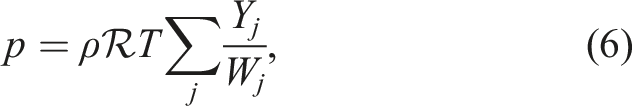
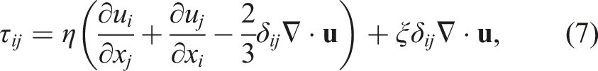
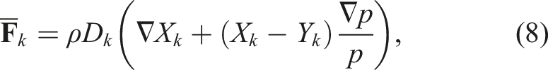
The system of equations for this model uses the multicomponent reacting compressible Navier–Stokes equations given as

\begin{array}{l} \frac{\partial ρ}{\partial t} & = - \nabla \cdot (ρ u), \end{array}

(5a)

\begin{array}{l} \frac{\partial ρ Y_{k}}{\partial t} & = - \nabla \cdot (ρ Y_{k} u) + ρ {\dot{ω}}_{k} - \nabla \cdot F_{k}, \end{array}

(5b)

\begin{array}{l} \frac{\partial ρ u}{\partial t} & = - \nabla \cdot (ρ uu) - \nabla p + \nabla \cdot τ, \end{array}

(5c)

\begin{array}{l} \frac{\partial ρ E}{\partial t} = - \nabla \cdot [(ρ E + p) u] + \nabla \cdot λ \nabla T \\ + \nabla \cdot (τ \cdot u) - \nabla \cdot \sum_{k} F_{k} h_{k} \end{array}

(5d)

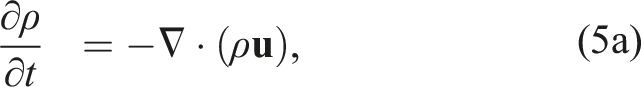
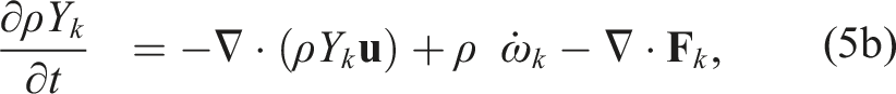
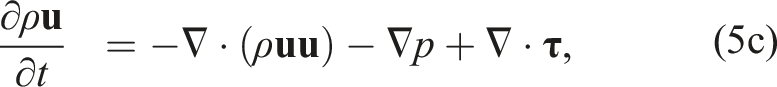
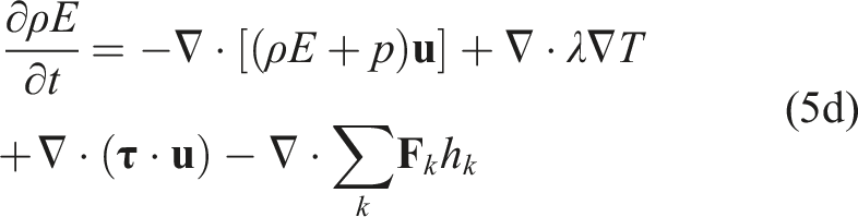
Here, ρ is the density, u is the velocity, p is the pressure, E is the specific energy density (kinetic plus internal), T is the temperature, τ is the viscous stress tensor, and λ is the thermal conductivity. For each of the chemical species k, Y_k is the mass fraction, F_k is the diffusive flux, h_k is the specific enthalpy, and ${\dot{ω}}_{k}$ is the production rate. The system is closed by an ideal gas mixture equation of state that specifies p as a function of ρ, T, and Y_k,

p = ρ R T \sum_{j} \frac{Y_{j}}{W_{j}},

(6)

where

R

is the universal gas constant and W_j is the molecular weight of species j. We use the standard full form of the viscous stress tensor,

τ_{i j} = η (\frac{\partial u_{i}}{\partial x_{j}} + \frac{\partial u_{j}}{\partial x_{i}} - \frac{2}{3} δ_{i j} \nabla \cdot u) + ξ δ_{i j} \nabla \cdot u,

(7)

where η is the shear viscosity and ξ is the bulk viscosity. The species diffusion flux is given by

{\bar{F}}_{k} = ρ D_{k} (\nabla X_{k} + (X_{k} - Y_{k}) \frac{\nabla p}{p}),

(8)

where X_k is the mole fraction and D_k is the diffusion coefficient of species k. In order to ensure mass is conserved, we impose a constraint that the sum of the species diffusion fluxes must equal zero. We enforce this constraint using a correction velocity technique that modifies these fluxes with a mass-fraction weighted correction that ensures this constraint is satisfied, as commonly used in combustion algorithms and described in Emmett et al. (2014).

In the second model, we compute the evolution of the mass fractions due to advection, diffusion, and reactions. We use a simplified advective and diffusive transport model where we hold velocity, density, pressure, and the diffusion coefficient constant. The governing equation for the mass fractions is

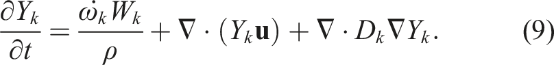
\frac{\partial Y_{k}}{\partial t} = \frac{\dot{ω_{k}} W_{k}}{ρ} + \nabla \cdot (Y_{k} u) + \nabla \cdot D_{k} \nabla Y_{k} .

(9)

Unlike the first model, this system is not taken from another study but was constructed to exercise the methods discussed in this paper. We develop this model as it allows for testing of various MRI schemes using three-component mixed implicit-explicit systems as in equation (2), and it serves as a proxy for the fully reacting flow problems we also consider. The state-dependent diffusion coefficients in the first model require a more complex approach to implicit discretization that is beyond the scope of this paper.

3.1. Spatial discretization

The spatial discretization for the tests in Section 5 integrates equation (5a)–(5d) with a finite difference approach with a uniform, single-level grid structure as described in Emmett et al. (2014). Centered, compact eighth-order spatial stencils are used in the interior of the domain, which require four cells on each side of a point where a derivative is computed. As all calculations in our tests were done in parallel using spatial domain decomposition, four ghost cells are exchanged between each spatial partition when computing derivatives (see Section 4.1). Stencils near non-periodic physical domain boundaries are handled as follows. Cells four away from a physical boundary use sixth-order centered stencils. Cells three away use fourth-ordered centered stencils. At cells two away, diffusion stencils use a centered second-order stencil while advection stencils use a biased third-order stencil. For the boundary cell, diffusion uses a completely biased second-order stencil and advection a wholly biased third-order stencil. While this mixture of discretizations theoretically results in overall second-order spatial accuracy, we replicate it here to allow for direct comparisons against the results from Emmett et al. (2014).

The advection and diffusion operators for the tests in Section 6 integrate the model in equation (9) and are discretized using standard second-order finite-volume stencils. These stencils require that one ghost cell be exchanged between spatial partitions during parallel computation of derivatives. Test problems using this model all used periodic boundary conditions, so the stencils remain second-order at physical boundaries.

3.2. Temporal discretization

In this work, we explore a third-order explicit MRI method, as well as third- and fourth-order solve-decoupled IMEX-MRI-GARK methods. The overall cost at the fast time scale for each method is commensurate with a single sweep over the time interval, while the overall cost at the slow time scale is commensurate with a standard additive Runge–Kutta IMEX (ARK-IMEX) method (Ascher et al., 1995). We compare their performance on the two model problems against single-rate and multirate SDC methods, as well as a standard ARK-IMEX method. The configuration and rough operation counts for a single step of each of the methods are as follows:

• SDC: Explicit fourth-order single-rate SDC method that uses a 3-point quadrature and four iterations per step.

• MRSDC-338: Explicit fourth-order multirate SDC method reported in Emmett et al. (2014). Uses a 3-point quadrature for f^S, a 3-point quadrature repeated 8 times per iteration for f^F, and four iterations per step.

• MRSDC-352: Explicit fourth-order multirate SDC method reported in Emmett et al. (2014). Uses a 3-point quadrature for f^S, a high-order 5-point quadrature repeated only twice per iteration for f^F, and four iterations per step.

• MRI3: The slow method is the third-order explicit method from Knoth and Wolke (1998) that requires four evaluations of f^S and evolution of four modified fast IVPs (equation (3)). At the fast time scale, we use explicit Runge–Kutta methods of orders two through five, corresponding to Heun, Bogacki and Shampine (1989) without use of the second-order embedding, Zonneveld (1963), and Cash and Karp (1990), respectively.

• ARK-IMEX: A fourth-order single-rate ARK-IMEX Runge–Kutta method from Kennedy and Carpenter (2003). Each step requires six evaluations of f^E and the solution of five diagonally-implicit nonlinear systems using f^I.

• IMEX-MRI3: The slow method is the IMEX-MRI-GARK3b method from Chinomona and Reynolds (2021), and the fast method is Kutta’s third-order method (Kutta, 1901). Within each slow-time step, this approach requires four evaluations of f^E, the solution of three diagonally-implicit nonlinear systems using f^I, and the evolution of three modified fast IVPs (equation (3)).

• IMEX-MRI4: The slow method is the IMEX-MRI-GARK4 method from Chinomona and Reynolds (2021), and the fast method is the classic fourth-order Runge–Kutta method. Within each slow-time step, this approach requires six evaluations of f^E, the solution of five diagonally-implicit nonlinear systems using f^I, and the evolution of five modified fast IVPs (equation (3)).

The model problem of equation (5a)–(5d) is simulated using the multirate MRSDC-338, MRSDC-352, and MRI3 methods, plus the single-rate SDC. The right-hand side is kept unpartitioned for SDC but is divided into fast and slow partitions for the multirate methods (both MRSDC and MRI). Since the simulation accuracy for all approaches hinges on resolution of the chemistry, the multirate methods put the chemical reaction term in equation (5b) into the fast partition, $f^{F} = ρ {\dot{ω}}_{k}$ , and the remaining transport terms are put into the slow, f^S. SDC must use the same step size for the transport as needed to accurately resolve the chemistry, whether that is necessary for them or not.

Problem (9) is computed with the multirate IMEX-MRI3 and IMEX-MRI4 methods, as well as the standard ARK-IMEX method. For the same reason as the previous problem, the multirate integrators place the chemical reaction term into the fast partition, $f^{F} = \frac{{\dot{ω}}_{k} W_{k}}{ρ}$ . The remaining slow terms are split into an explicitly stepped partition containing the advection term, f^E = ∇ ⋅ (Y_ku), and an implicitly stepped one with the diffusion term, f^I = ∇ ⋅ D_k∇Y_k. For ARK-IMEX, the chemistry and advection are assigned to the explicit partition, f^E, and the diffusion to the implicit one, f^I. In that method, all partitions are stepped at the step size needed to resolve the chemistry, even if it is smaller than needed for the transport.

4. Implementation

Our implementation uses the AMReX (Zhang et al., 2019, 2021) adaptive mesh refinement library and its predecessor package, BoxLib (Zhang et al., 2016), for spatial discretizations and the SUNDIALS library (Gardner et al., 2022; Hindmarsh et al., 2005; Reynolds et al., 2023) for temporal discretizations. Interfacing SUNDIALS with BoxLib allowed for an easier, direct comparison to previously developed code, and interfacing SUNDIALS with AMReX demonstrates the interoperability of the two libraries.

4.1. Block-structured meshes

AMReX is a software framework that supports the development of block-structured AMR algorithms for solving systems of partial differential equations on current and emerging architectures. AMReX supplies data containers and iterators for mesh-based fields, supporting data fields of any nodality. There is no parent-child relationship between coarser grids and finer grids. See Figure 2 for a sample grid configuration. In order to create refined grids, users define “tagging” criteria to mark regions where refined grids are necessary. The tagged cells are grouped into rectangular grids using the clustering algorithm in Berger and Rigoutsos (1991). There are user-defined parameters controlling the maximum length a grid can have, as well as forcing each side of the grid to be divisible by a particular factor. Furthermore, grids can be subdivided if there is an excess of MPI processes with no load. Proper nesting is enforced, such that a fine grid is strictly contained within the grids at the next-coarser level.

Figure 2.

In block-structured AMR, there is a hierarchy of logically rectangular grids. The computational domain on each AMR level is decomposed into a union of rectangular domains. In this figure, there are three total levels. The coarsest “level 0” grid covers the domain; bold red lines represent grid boundaries. The green “level 1” grids contain cells that are a factor of two (or optionally four) finer than those at level 0. The blue “level 2” grids contain cells that are a factor of two (or four) finer than those at level 1. Note that there is no direct parent-child connection.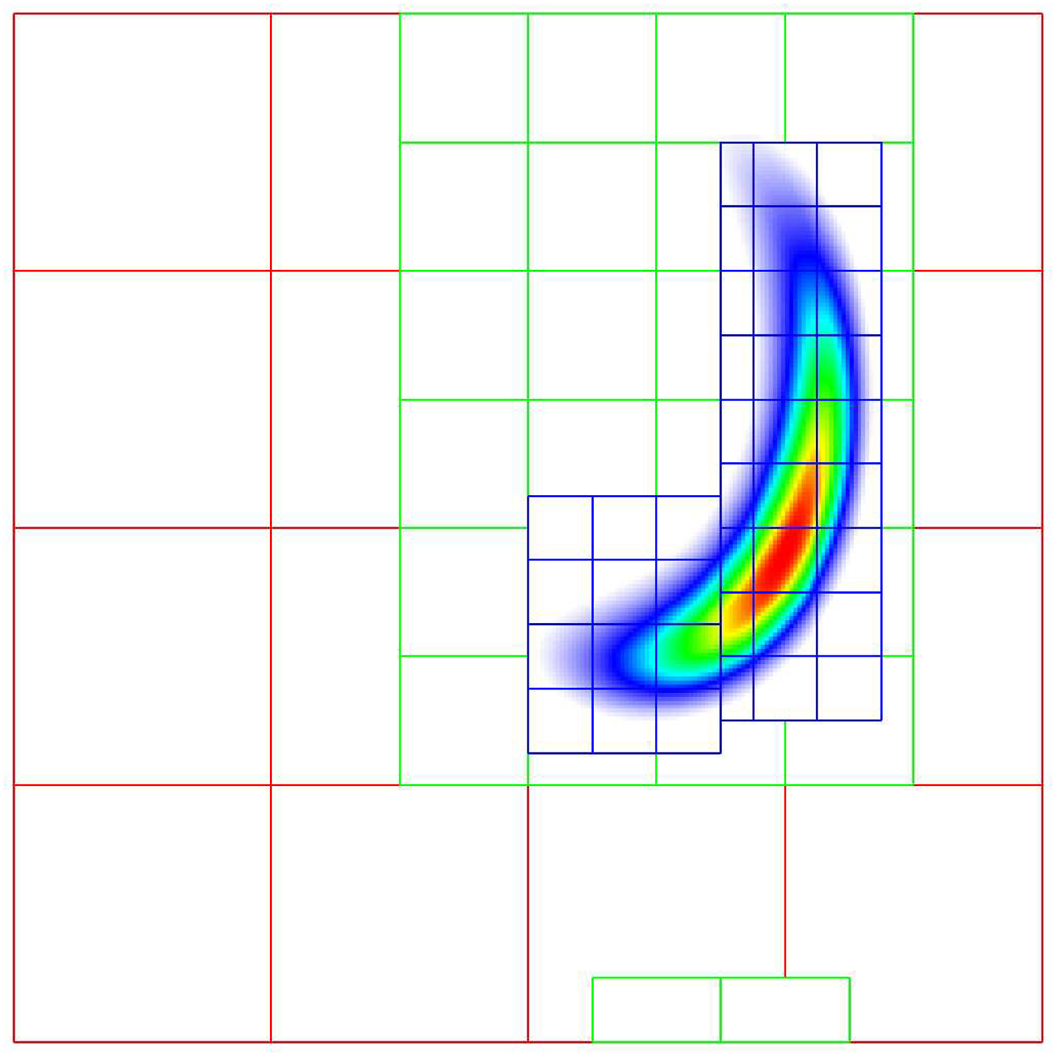

In this work, we leverage (a) performance enhancements in the context of single-core and MPI performance; (b) built-in grid generation, load balancing, and multilevel communication patterns; (c) linear solvers via geometric multigrid; (d) efficient parallel I/O; and (d) visualization support through VisIt, ParaView, and yt. The functionality in AMReX makes it easy to efficiently solve for the implicit terms in IMEX methods and is straightforward to use with both single-level and multi-level grids. The spatial discretization for the first model is implemented in the pure Fortran90 BoxLib framework, as was done in Emmett et al. (2014). The second model is used for testing IMEX-MRI-GARK methods. Because the problem is a mostly new implementation and uses a different spatial discretization and implementation, it takes advantage of the most updated version of AMReX for the spatial discretization and multigrid preconditioning (where used) while retaining the complex chemistry from the first problem. In both cases, the chemistry uses the same Fortran implementation while SUNDIALS is used for timestepping.

AMReX uses an MPI + X strategy where grids are distributed over MPI ranks, and X represents a fine-grained parallelization strategy. In recent years, the most common X in the MPI + X strategy has been OpenMP, but AMReX also has been extended to support GPU computing on NVIDIA, AMD, and Intel GPUs. The focus in this paper is on pure MPI. Future efforts will be able to easily adopt the multicore/GPU strategies by using AMReX’s built-in ParallelFor iterators. In the multicore CPU case, AMReX box iterators are used to walk over local tiles within each box, where threading (if used) can be assigned to individual tiles to operate in parallel. In the GPU case, AMReX ParallelFor iterators are instead used to walk the local cells of the box in parallel, and the discretization is applied in the form of a C++ lambda with each cell being assigned to an individual GPU thread. Converting from the single-threaded case is usually no more than replacing the C++ for loops over the cells with a ParallelFor line and copying the body of the discretization into a lambda. Further details about AMReX’s multicore/GPU strategy can be found in Zhang et al. (2021).

Load balancing over MPI ranks is done on a level-by-level basis using either a Morton-order space filling curve or knapsack algorithm. AMReX efficiently manages and caches communication patterns between grids at the same level, grids at different levels, as well as data structures at the same level with different grid layouts. The latter case is useful when certain physical processes have widely varying computational requirements in different spatial regions, and grid generation with load balancing in mind may be weighted by this metric, rather than cell count.

4.2. Time integrators

The MRI methods evaluated in this work are provided by the SUNDIALS suite of time integrators and nonlinear solvers (Gardner et al., 2022; Hindmarsh et al., 2005). The suite is comprised of the ARKODE package of one-step methods for ODEs, the multistep integrators CVODE and IDA for ODEs and DAEs, respectively, the forward and adjoint sensitivity analysis enabled variants, CVODES and IDAS, and the nonlinear algebraic equation solver KINSOL. The ARKODE package provides an infrastructure for developing one-step methods for ODEs and includes time integration modules for stiff, non-stiff, mixed stiff/non-stiff, and multirate systems (Reynolds et al., 2023). ARKODE’s MRIStep module implements explicit MIS methods and high-order explicit and solve-decoupled implicit and IMEX MRI-GARK methods. In this work, we solve each fast-time scale ODE, equation (3), using ARKODE’s ARKStep module, which provides explicit, implicit, and ARK-IMEX Runge–Kutta methods, though a user may also provide their own fast-scale integrator. The specific MRI methods evaluated in this work are built into ARKODE, but users may alternatively supply their own coupling tables for MRI methods or Butcher tables for Runge–Kutta methods. At a minimum, to utilize the methods in ARKODE, an application must provide routines to evaluate the ODE right-hand side functions, and ARKODE must be able to perform vector operations on application data.

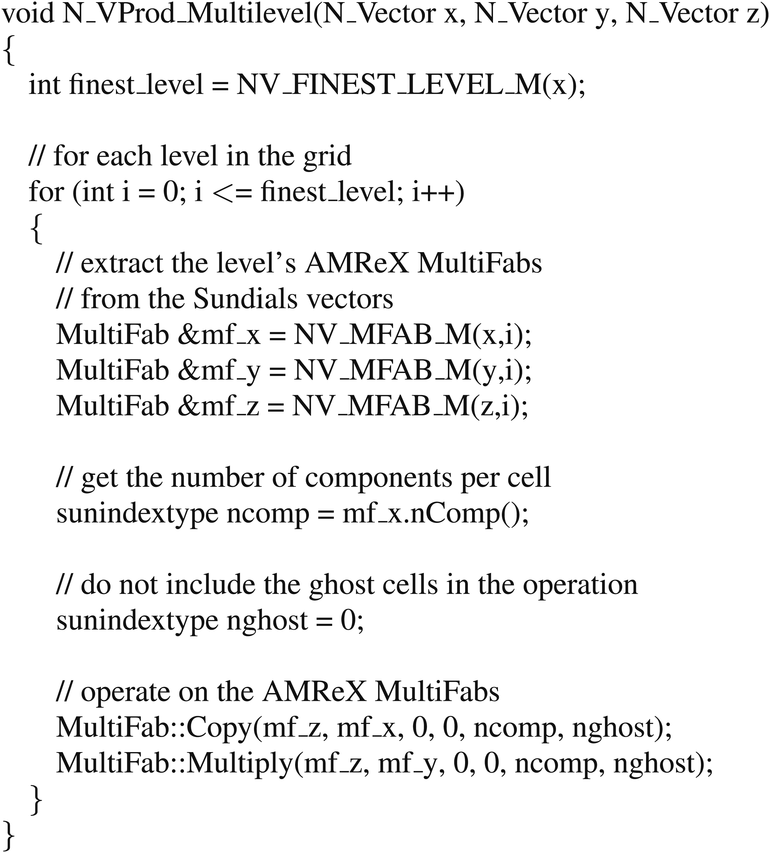
SUNDIALS packages utilize an object-oriented design and are written in terms of generic mathematical operations defined by abstract vector, matrix, and solver classes. Thus, the packages are agnostic to an application’s particular choice of data structures/layout, parallelization, algebraic solvers, etc. as the specific details for carrying out the required operations are encapsulated within the corresponding classes. Several vector, matrix, and solver modules are provided with SUNDIALS, but users can also provide their own class implementations tailored to their use case. In this work, we supplied custom vector implementations to interface with the native BoxLib and AMReX data structures (one for BoxLib in Fortran, one each for the single- and multi-level grid cases of AMReX in C++). Often, in-built functionality from BoxLib or AMReX could be used to aid these routines, but sometimes the cells in the grid needed to be iterated over and the operation computed per-cell explicitly. The following is the listing for the vector multiplication operation (multiplies per-element like Matlab’s .* operation) that leverages in-built AMReX operations in the multi-level case:

With explicit MRI methods, as used in the first problem of equation (5a)–(5d), a vector implementing the necessary operations and routines for evaluating the right-hand side functions is all that is required for interfacing with SUNDIALS. For the IMEX-MRI methods, as used in the second problem of equation (9), a nonlinear solver and a linear solver are needed to solve the nonlinear systems that arise at each implicit slow stage. Here, we use the native SUNDIALS Newton solver and matrix-free GMRES implementation to solve these algebraic systems. As both solvers are written entirely in terms of vector operations, no additional interfacing is required. However, to accelerate convergence of the GMRES iteration, an additional wrapper function was created to leverage the AMReX multigrid linear solver as a preconditioner. This solver is based on the “MLABecLaplacian” linear operator,

(α I - \nabla \cdot β \nabla) ϕ = R,

(10)

where α and β are spatially-varying coefficients.

5. Explicit time stepping on compressible reacting flow

The results in this section are motivated by earlier success of the explicit MRSDC methods on the SMC combustion problem (Emmett et al., 2014) in equation (5a)–(5d). Here, we compare the performance of various MRI and MRSDC methods on this same model and discuss how their structural differences affect their relative performance.

5.1. Problem setup

The experiment in this section is close in configuration to the three-dimensional methane flame problem from Section 5.2.2 in Emmett et al. (2014). The problem domain is a cubic box 1.6 cm on each side. The boundaries are periodic in the y and z directions and inlet/outlet in the x-direction. The chemistry mechanism for the flame is the GRI-MECH 3.0 network (Frenklach et al., 1995) that contains 53 species and 325 reactions. Combined with the other state variables, such as density and velocity, the resulting system has 58 unknowns at each spatial location. The initial conditions are taken from the PREMIX code from the CHEMKIN library (Kee et al., 1998), where we use a precomputed realistic distribution of species in a premixed methane flame in 1D along the x-axis with offsets in the pattern varying in the y-z plane by perturbing spherical harmonics, resulting in a bumpy but smoothly continuous pattern at the front. The problem is integrated over a total time of t = 2.0 × 10⁻⁶ s using coarse time step sizes that range from H = 2.0 × 10⁻⁶ to H = 1.5625 × 10⁻⁸ s. We note that the problem remains smooth over the entire time interval and does not form shocks.

The domain interior is discretized with 32³ points. Since there are 58 unknowns per spatial location, this discretization gives a total of 1,900,544 unknowns over the interior of the domain. The problem is parallelized by splitting each dimension in half, resulting in 8 boxes distributed over 8 MPI ranks. Since the discretization also requires an additional four layers of ghost cells at each face, the total number of data in the problem becomes 6,414,336 values when including ghost cells.

As with Emmett et al. (2014), we test this problem on the single-rate SDC and the two multirate SDC methods, MRSDC-338 and MRSDC-352. Here, we also compare against MRI3. As noted in Section 3.2, the MRI3 scheme is paired with fast methods of orders two through five. For each method, we perform k fast substeps per slow step (where that ratio is held constant over the problem) and denote the resulting combinations as MRI-P(k), where P is the order of the fast method. Through exhaustive testing on this application, we found the following options to be the most efficient for each fast-method order: MRI-2(8), MRI-3(4), MRI-4(8), and MRI-5(4).

The accuracy of the methods is tested against a reference solution calculated using a six-stage fourth-order explicit Runge–Kutta method (Kennedy et al., 2000) with a step size of 5.0 × 10⁻¹⁰ s. Note that as with the corresponding test in Emmett et al. (2014), the reference solution is computed at the same spatial resolution as for the integrator tests. As such, the measured error is for the time integration error relative to the system of ODEs produced from first applying the spatial discretization.

The results were gathered on a node of the Quartz cluster at Lawrence Livermore National Laboratory. Each node is composed of two Intel Xeon E5-2695 v4 chips. The tests used 8 ranks of MPI parallelism distributed over the cores of the node.

5.2. Results

The range of magnitudes of the different solution components (e.g., density, velocity, and mass fractions of different species) is quite large in this problem, so a norm of error over the solution would not properly capture the total error over all components without using an appropriate weighting vector in the norm. As in Emmett et al. (2014), we find the order of convergence of the methods to not depend on which solution component is chosen. Therefore, rather than using a norm over all components, we measure the error as the max norm in density. The results are similar for other components.

The integration of each method is done using constant time stepping, starting each with the coarsest time step that exhibited numerical stability and halving the step for each successive run. The coarsest allowable time step for each method can be seen in Table 1. Not included in the table is the single-rate SDC case, which required a step size no greater than 6.25 × 10⁻⁸ s to be stable. We note that the single-rate restriction of

O (10^{- 8})

is consistent with the analysis of the eigenvalues in the Jacobian of this reaction network (Wartha et al., 2020). We also note that the acoustic CFL time step limit is

H \sim O (10^{- 6})

s, so both our reference solution and test simulations use a time step far smaller than this due to the stiffness of the chemistry.

Table 1.

L_∞ error and convergence rates for density using various multirate approaches on a methane flame test from Section 5. The omitted values for largest time steps indicate simulations that became unstable and were unable to finish.

Method	MRSDC338		MRSDC352		MRI-2(8)		MRI-3(4)		MRI-4(8)		MRI-5(4)
H (s)	L_∞ error	Rate	L_∞ error	Rate	L_∞ error	Rate	L_∞ error	Rate	L_∞ error	Rate	L_∞ error	Rate
2.0× 10⁻⁶	1.80 × 10⁻²
1.0 × 10⁻⁶	2.73 × 10⁻³	2.72					5.50 × 10⁻³
5.0 × 10⁻⁷	2.81 × 10⁻⁴	3.28			8.40 × 10⁻³		2.17 × 10⁻⁴	4.48	1.03 × 10⁻³
2.5 × 10⁻⁷	4.94 × 10⁻⁵	2.51	4.95 × 10⁻³		3.72 × 10⁻⁴	4.50	1.79 × 10⁻⁴	0.27	1.21 × 10⁻⁴	3.09	7.77 × 10⁻⁴
1.25 × 10⁻⁷	1.17 × 10⁻⁵	2.07	3.44 × 10⁻⁵	7.17	4.07 × 10⁻⁵	3.20	6.07 × 10⁻⁵	1.56	4.63 × 10⁻⁶	4.71	1.48 × 10⁻⁵	5.71
6.25 × 10⁻⁸	3.62 × 10⁻⁶	1.69	2.12 × 10⁻⁶	4.02	9.06 × 10⁻⁷	5.89	4.31 × 10⁻⁶	3.81	4.61 × 10⁻⁷	3.33	1.15 × 10⁻⁶	3.68
3.125 × 10⁻⁸	2.12 × 10⁻⁶	0.77	4.19 × 10⁻⁹	8.98	4.12 × 10⁻⁸	4.46	1.18 × 10⁻⁷	5.20	4.12 × 10⁻⁸	3.48	4.12 × 10⁻⁸	4.80
1.5625 × 10⁻⁸	2.01 × 10⁻⁶	0.08	1.77 × 10⁻⁹	1.24	5.02 × 10⁻⁹	3.04	4.95 × 10⁻⁹	4.57	4.96 × 10⁻⁹	3.05	4.96 × 10⁻⁹	3.05

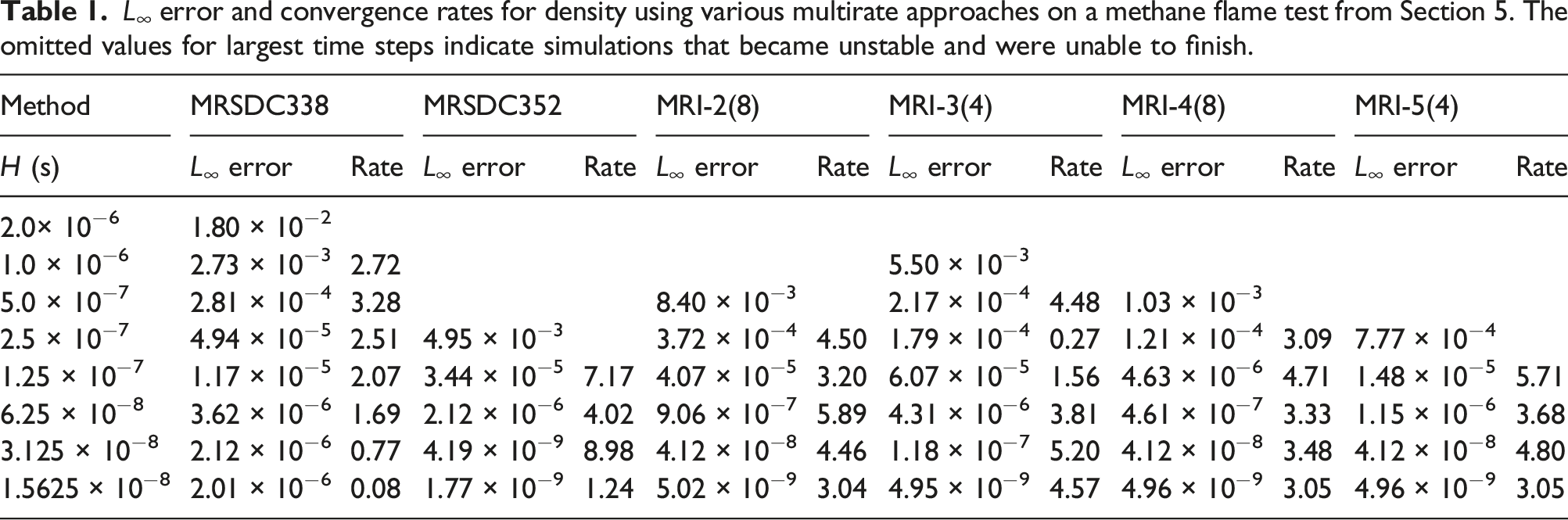
The rate of convergence for each of the methods is shown in Figure 3, and the same data is shown in tabular form in Table 1. In general, the MRSDC methods exhibit highly non-monotonic convergence rates, despite their theoretical fourth-order accuracy. This problem could possibly be alleviated by further reducing the step size, or increasing the number of SDC iterations, as has been demonstrated in other works using SDC for reacting flow (Nonaka et al., 2012, 2018; Pazner et al., 2016). The rate of convergence of the MRI methods is a balance between the accuracy of the fast and slow partitions. The MRI-4 and MRI-5 methods are asymptotically limited to third-order accuracy due to the third-order accuracy of the slow integrator; however, the slope of the convergence plot is better than four in some ranges when the reactions dominate the overall accuracy. The MRI-2 method is asymptotically limited to only second-order as step sizes become small, but the slope of the line is at least three for the ranges of step sizes used in the tests. Overall, the MRI methods exhibit convergence rates consistent with the expected order of accuracy and appear to reach the asymptotic range of convergence at larger step sizes than the MRSDC approaches.

Figure 3.

Error in each method versus time step for the explicit methods from Section 5. Each of the MRI methods exhibits at least third-order accuracy as expected. The convergence rates for the MRSDC approaches are highly non-monotonic.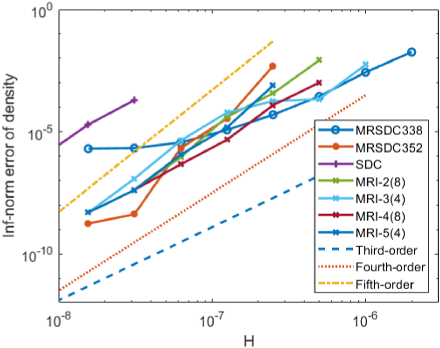

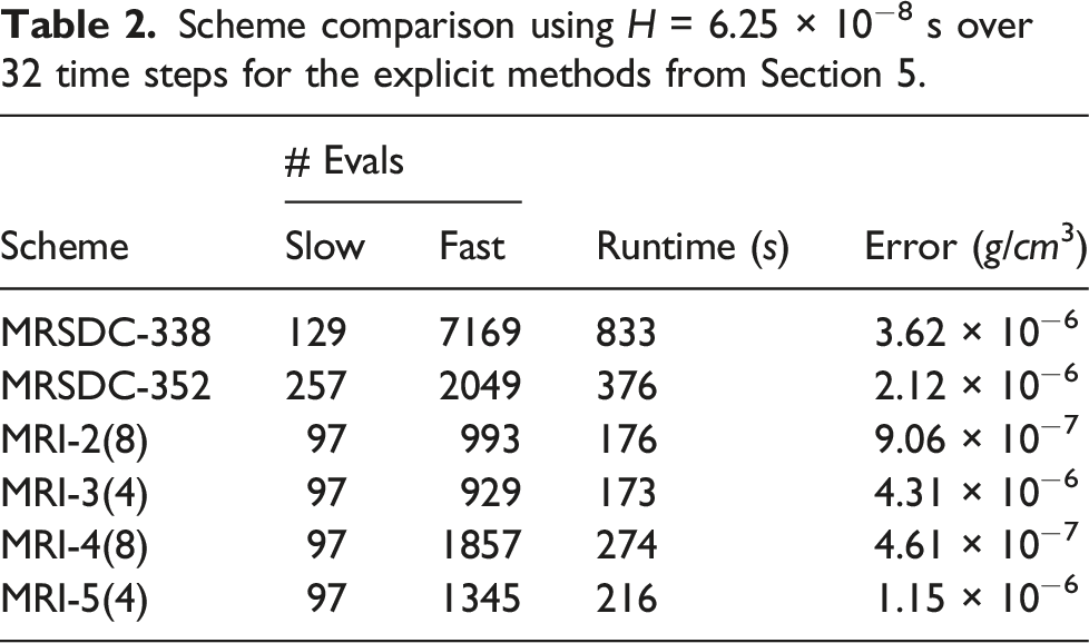
Figure 4 shows an efficiency diagram comparing the performance of the various integrators, plotting the error in density as a function of wallclock time. The figure confirms the results of Emmett et al. (2014) that the MRSDC methods have a significant performance advantage over the single-rate SDC method on this problem. We also see that, in general, the MRI methods produce smaller error for a given wallclock time compared to the SDC approaches. The exception is for the smallest step sizes reported, the MRSDC352 4-iteration performs comparably to the MRI approaches. As discussed in Section 2.2, the performance benefits of MRI approaches arise because the MRI methods need fewer calls to the right-hand-side functions per step than the SDC methods. To further quantify this point, Table 2 presents the H = 6.25 × 10⁻⁸ s data from Figure 4 and Table 1, including the number of function calls, runtime, and error using four different approaches. The error for the MRI approaches is comparable to or smaller than the SDC approaches, in addition to offering runtimes that are notably smaller due to the reduced number of slow and fast evaluations.

Figure 4.

Error in each method versus CPU time for the explicit methods from Section 5.

Table 2.

Scheme comparison using H = 6.25 × 10⁻⁸ s over 32 time steps for the explicit methods from Section 5.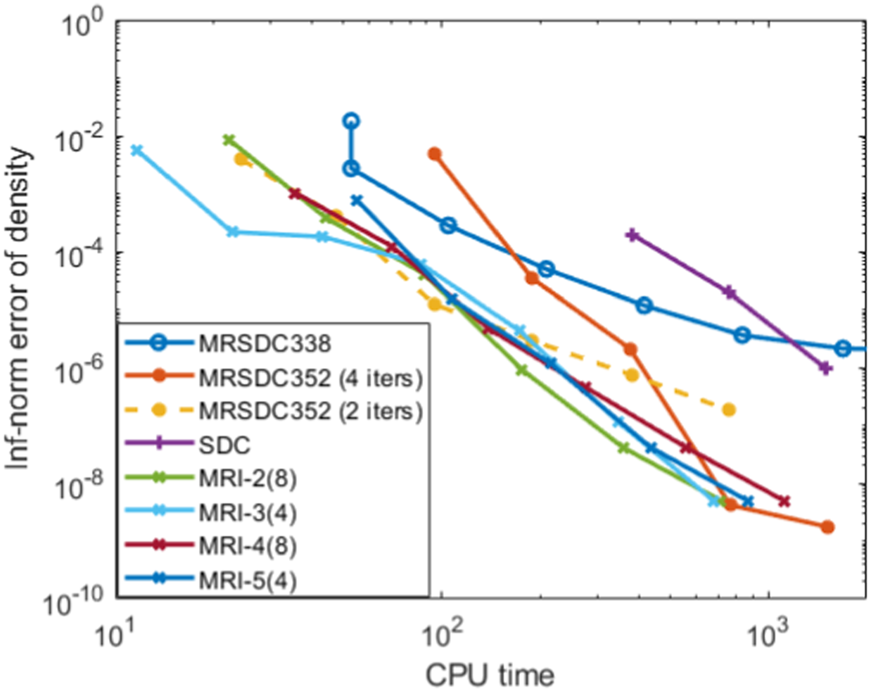

Scheme	# Evals		Runtime (s)	Error (g/cm³)
Scheme	Slow	Fast	Runtime (s)	Error (g/cm³)
MRSDC-338	129	7169	833	3.62 × 10⁻⁶
MRSDC-352	257	2049	376	2.12 × 10⁻⁶
MRI-2(8)	97	993	176	9.06 × 10⁻⁷
MRI-3(4)	97	929	173	4.31 × 10⁻⁶
MRI-4(8)	97	1857	274	4.61 × 10⁻⁷
MRI-5(4)	97	1345	216	1.15 × 10⁻⁶

6. IMEX time stepping on a reacting flow problem implemented in AMReX

For IMEX multirate tests, we use the simplified model defined by equation (9). The chemistry reaction mechanism is the same as for the compressible reacting flow problem of Section 5. However, here the diffusion term is much stiffer to represent the type of diffusive stiffness that must be confronted on large-scale transport problems. The advection term is non-stiff. As with the previous problem, the chemistry uses a small timestep to resolve the fast dynamics and the transport uses coarse time steps, but now the diffusion term must be handled implicitly to deal with its stiffness.

6.1. Problem setup

The problem domain is a 3D cube [−0.05, 0.05] cm on a side with periodic boundaries in each direction. The chemistry mechanism is the same GRI-MECH 3.0 network (Frenklach et al., 1995) as the previous problem (53 species, 325 reactions). The model is integrated over a total time of t = 2.0 × 10⁻⁶ s.

The problem is initialized using the same predetermined realistic distribution of species in 1D for a fuel mix as that used in the previous example. However, here the 1D distribution is swept angularly around the origin with high concentration offset from the middle, resulting in a ring of fuel centered around the center. The temperature is set as 1500 K everywhere, the pressure is set at 1 atmosphere everywhere, and the density is calculated from the standard equation of state from the pressure and temperature at each cell. The velocity of the system is ⟨0.001, 0.001, 0.001⟩ cm/s uniformly across the domain. This problem also remains smooth over the entire time interval and does not form shocks.

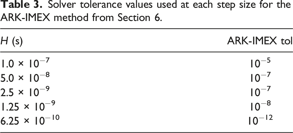
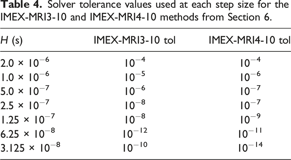
The problem is tested using ARK-IMEX, IMEX-MRI3, and IMEX-MRI4. Details of the methods and the partitioning of the model terms are described in Section 3.2. The time stepping is done with constant step sizes, with 10 fast steps taken for each slow step in the multirate methods. The multirate methods are thus labeled as “IMEX-MRI3-10” and “IMEX-MRI4-10” in what follows.

For the implicit partitions, the implicit stage solves are done using SUNDIALS’ Newton iteration and matrix-free GMRES solver. No preconditioning is used. To prevent iterations being terminated before reaching tolerance, the maximum number of nonlinear and linear iterations (per nonlinear iteration) is relaxed from the default to 10 and 100, respectively. However, solver tolerances also need to be set for the nonlinear and linear solvers in order to avoid “over-solving” the algebraic systems of equations as well. The nonlinear solver tolerances were chosen on a per-method and per-timestep size basis. The chosen solver tolerance values are listed in Table 3 and Table 4. The reported values were chosen by sweeping each case over a range of tolerances from 10⁻¹ to 10⁻¹⁵, with jumps of a factor of 10 between each, with the reported value being the coarsest one for which both the H2 and H mass fraction error is perturbed by less than a factor of 0.01. The tolerance value is used as an absolute tolerance in the WRMS norm for the nonlinear solver and the 2-norm for the linear solver over the entire solution vector, that is, over all species at once. Safety factors of 0.1 and 0.05 are applied for the nonlinear and linear solvers, respectively.

Table 3.

Solver tolerance values used at each step size for the ARK-IMEX method from Section 6.

H (s)	ARK-IMEX tol
1.0 × 10⁻⁷	10⁻⁵
5.0 × 10⁻⁸	10⁻⁷
2.5 × 10⁻⁹	10⁻⁷
1.25 × 10⁻⁹	10⁻⁸
6.25 × 10⁻¹⁰	10⁻¹²

Table 4.

Solver tolerance values used at each step size for the IMEX-MRI3-10 and IMEX-MRI4-10 methods from Section 6.

H (s)	IMEX-MRI3-10 tol	IMEX-MRI4-10 tol
2.0 × 10⁻⁶	10⁻⁴	10⁻⁴
1.0 × 10⁻⁶	10⁻⁵	10⁻⁶
5.0 × 10⁻⁷	10⁻⁶	10⁻⁷
2.5 × 10⁻⁷	10⁻⁸	10⁻⁷
1.25 × 10⁻⁷	10⁻⁸	10⁻⁹
6.25 × 10⁻⁸	10⁻¹²	10⁻¹¹
3.125 × 10⁻⁸	10⁻¹⁰	10⁻¹⁴

The reference solution is computed using the fifth-order explicit Runge–Kutta method from Cash and Karp (1990) with a step size of 10⁻¹⁰, which is an order of magnitude smaller than the smallest fast step size used in all the runs. As with the first test, the spatial resolution is the same as for the tests with the integrators, so the measured error is the temporal error for the system of ODEs resulting from first applying the spatial discretization.

The grid resolution is 128 cells on a side. Diffusion coefficients are computed in the same manner and library code as the SMC problem, using temperatures, molar fractions, and specific heat at constant pressure. The calculation of the diffusion coefficient is computationally expensive and dominates the cost of the implicit terms more than the nonlinear solves for the tested configuration of the problem. The coefficients are not updated within the solves, so the computational cost of that portion is not affected by the changes in iteration counts with stiffness. However, in order to make the problem sufficiently stiff to warrant an implicit method, the computed coefficient in each cell is scaled by a factor of 1000. The problem is thus not physically realistic but is meant to exercise the same code components that are expensive in a reactive-flow problem at a level of stiffness that would be found in highly resolved realistic cases. The scale of the diffusion coefficient combined with the grid resolution results in a problem that cannot be completed successfully using explicitly evolved diffusion at the coarser step sizes of the runs.

The problem is run with 512 total ranks over 16 nodes on the Quartz cluster at Lawrence Livermore National Laboratory.

6.2. Results

The results of the runs are shown in Figure 5. The error is shown for the species H2, but as with the SMC problem, the outcome is insensitive to which species is used to measure error.

Figure 5.

Efficiency diagrams for the IMEX methods from Section 6 with error measured for the H2 mass fraction.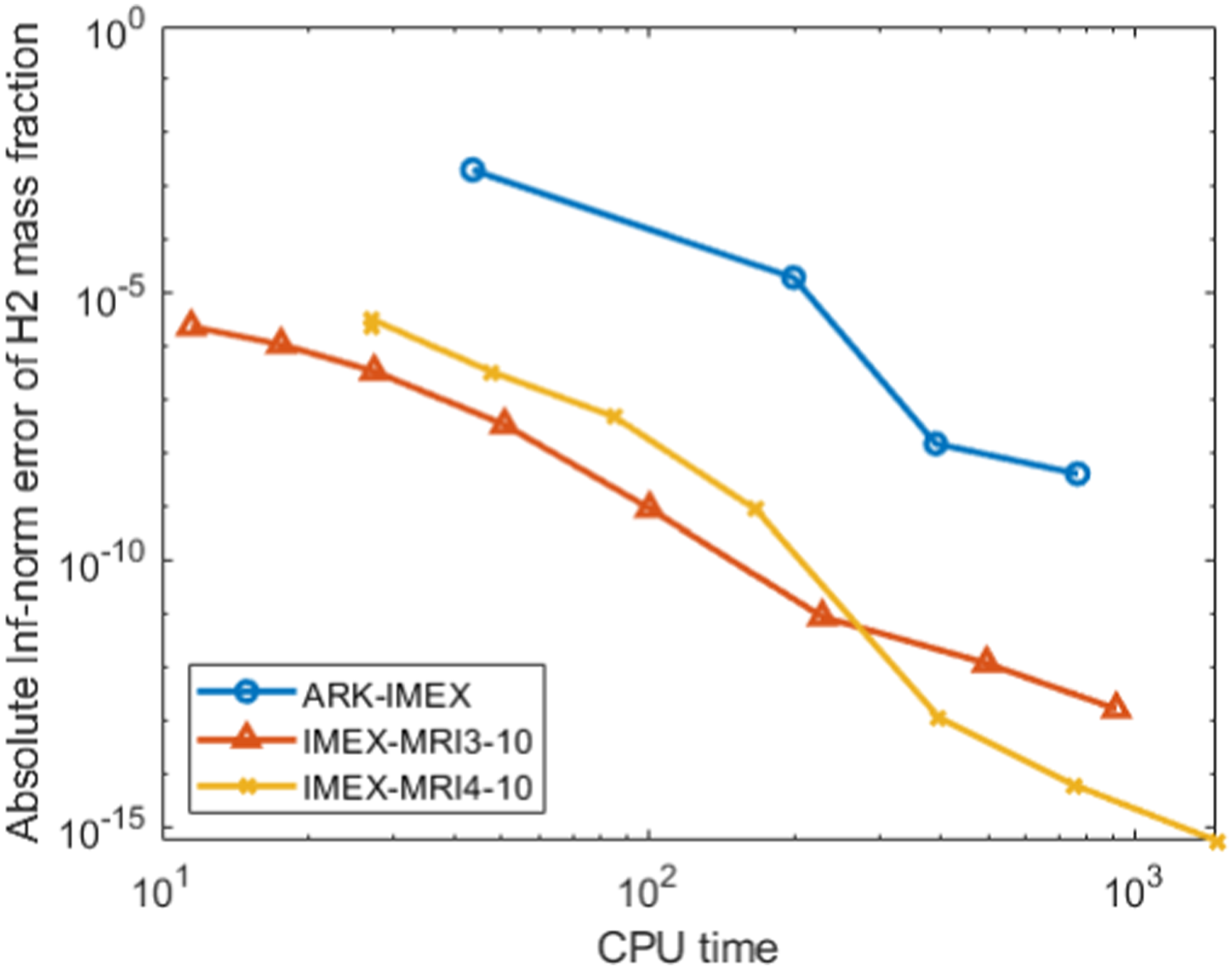

We see in the plots that there is a significant performance advantage when using multirate over single-rate IMEX methods for this problem. We tried the problem over a range of fast-to-slow step size ratios and found ten-to-one to be the best balance. Due to the expensive diffusion coefficient calculation, reducing the number of coarse steps that must be computed per fast step results in large time savings.

An interesting phenomenon from Tables 3 and 4 is that the solver tolerances needed by the multirate methods were more stringent than for the single-rate method for the same coarse step size. This seems to be due to the increased accuracy of the MRI solutions at those step sizes, thereby necessitating tighter algebraic solver tolerances.

Table 5 shows the scaling in CPU time and change in nonlinear and linear iterations for the problem as the grid resolution is refined. The results are from using the IMEX-MRI3-10 method over eight time steps, that is, at about mid-height in Figure 5. Even at a somewhat finer step size than the coarsest case, the problem is moderately stiff, so the number of linear iterations grows with the grid resolution. However, the primary cost is the computation of the diffusion coefficients, which are not done within the linear iterations. As a result, the total cost goes up only slowly with stiffness within the range of resolutions tested. If the problem were to continue to grow in size, eventually the solve cost would overtake the cost of the diffusion coefficient calculation, and a preconditioner would be needed. As mentioned in Section 4.2, AMReX includes the MLABecLaplacian multigrid solver that works over multiple AMR grid levels. Here, we use this preconditioner for this single-level problem, with results comparing the un-preconditioned and preconditioned solvers in Tables 5 and 6, respectively. Due to the overhead in invoking the preconditioner, for coarse problems the un-preconditioned solve is more efficient, but once the grid reaches at least 128 cells per side, the preconditioner becomes costeffective. Tables 7 and 8 push this experiment further, by artificially increasing the problem stiffness through scaling the diffusion coefficients by another factor of 10. Here again, preconditioning is effective at grid sizes exceeding 64 cells per side and becomes critical as the grids are increased to 256 cells per side.

Table 5.

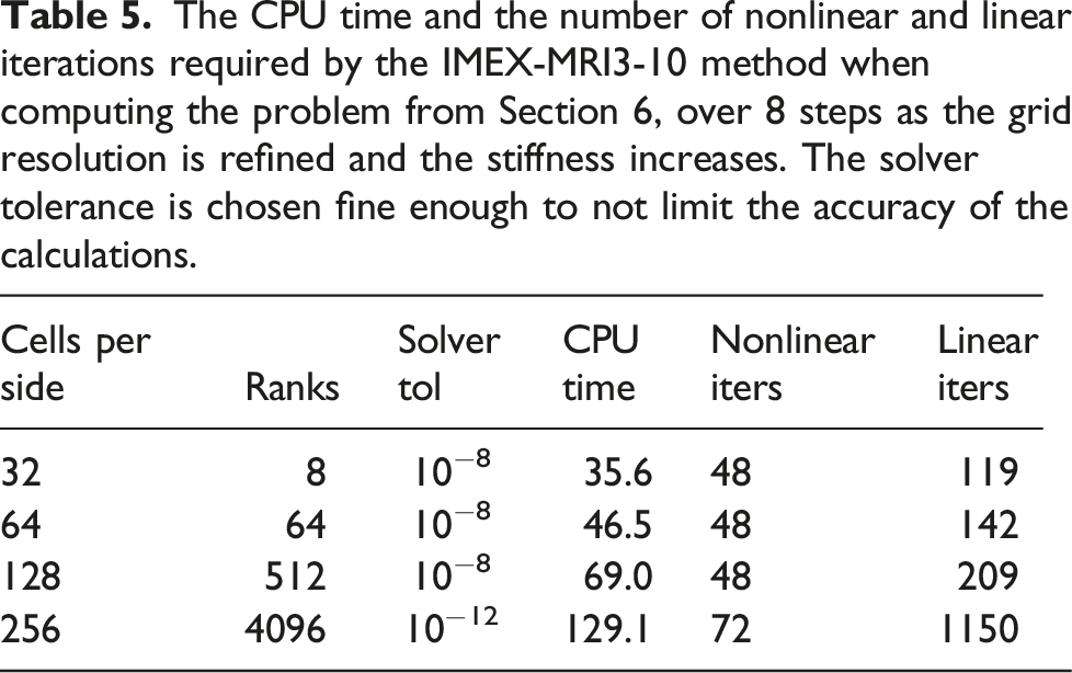
The CPU time and the number of nonlinear and linear iterations required by the IMEX-MRI3-10 method when computing the problem from Section 6, over 8 steps as the grid resolution is refined and the stiffness increases. The solver tolerance is chosen fine enough to not limit the accuracy of the calculations.

Cells per side	Ranks	Solver tol	CPU time	Nonlinear iters	Linear iters
32	8	10⁻⁸	35.6	48	119
64	64	10⁻⁸	46.5	48	142
128	512	10⁻⁸	69.0	48	209
256	4096	10⁻¹²	129.1	72	1150

Table 6.

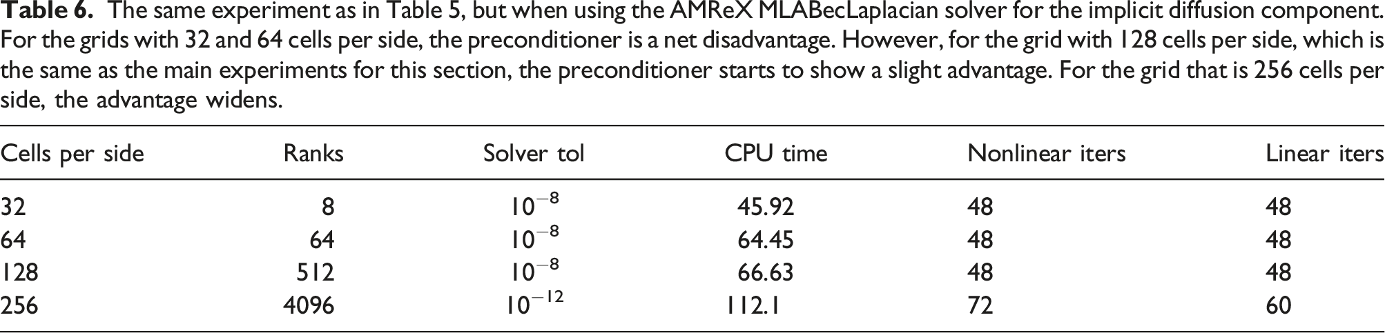
The same experiment as in Table 5, but when using the AMReX MLABecLaplacian solver for the implicit diffusion component. For the grids with 32 and 64 cells per side, the preconditioner is a net disadvantage. However, for the grid with 128 cells per side, which is the same as the main experiments for this section, the preconditioner starts to show a slight advantage. For the grid that is 256 cells per side, the advantage widens.

Cells per side	Ranks	Solver tol	CPU time	Nonlinear iters	Linear iters
32	8	10⁻⁸	45.92	48	48
64	64	10⁻⁸	64.45	48	48
128	512	10⁻⁸	66.63	48	48
256	4096	10⁻¹²	112.1	72	60

Table 7.

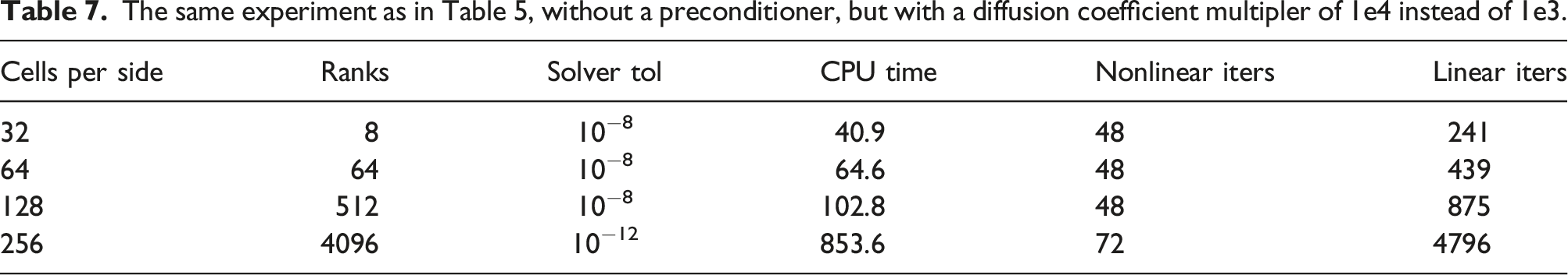
The same experiment as in Table 5, without a preconditioner, but with a diffusion coefficient multipler of 1e4 instead of 1e3.

Cells per side	Ranks	Solver tol	CPU time	Nonlinear iters	Linear iters
32	8	10⁻⁸	40.9	48	241
64	64	10⁻⁸	64.6	48	439
128	512	10⁻⁸	102.8	48	875
256	4096	10⁻¹²	853.6	72	4796

Table 8.

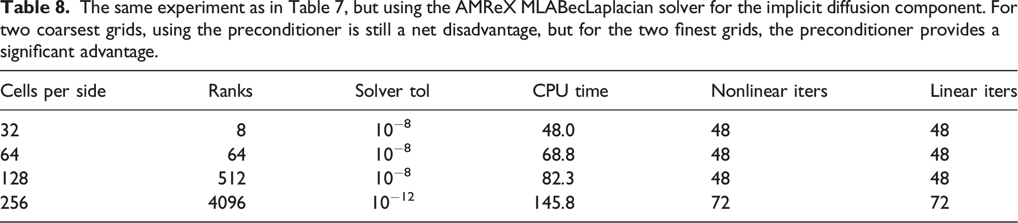
The same experiment as in Table 7, but using the AMReX MLABecLaplacian solver for the implicit diffusion component. For two coarsest grids, using the preconditioner is still a net disadvantage, but for the two finest grids, the preconditioner provides a significant advantage.

Cells per side	Ranks	Solver tol	CPU time	Nonlinear iters	Linear iters
32	8	10⁻⁸	48.0	48	48
64	64	10⁻⁸	68.8	48	48
128	512	10⁻⁸	82.3	48	48
256	4096	10⁻¹²	145.8	72	72

6.3. Simulation on multilevel grids

As a proof of concept and demonstration of capability, the problem of equation (9) is also implemented in AMReX on multi-level grids. The problem is initialized using the predetermined realistic distribution of species in 1D for a fuel mix as that used in the previous Section 5.1 but configured as a ball with methane fuel concentrated in the center. Otherwise, the problem is the same as from the single-level case. Figure 6 shows a 2D slice of the methane mass fraction at the initial time point, where we have overlaid boxes with coarser cell resolution (indicated in red) and boxes with finer cell resolution (indicated in black). The fine-resolution boxes overlay locations where there is a significant concentration of methane.

Figure 6.

Distribution of boxes in 3D overlaid on a 2D slice of the methane mass fraction at the initial time point. The cells within the black boxes have double the resolution of the cells within the red boxes.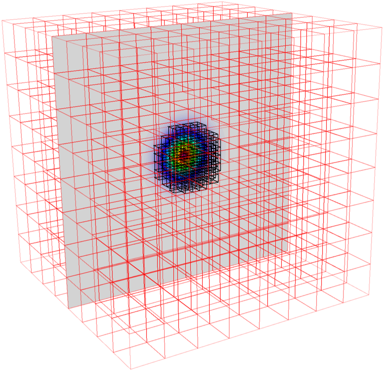

Unlike what is typically done with AMR, the multirate time stepping here is dictated by the accuracy requirements of the chemistry and diffusion and not by the CFL stability restriction. The advection is computed explicitly, but the velocity is too small in this problem for CFL limitations to restrict step sizes. The diffusion is computed implicitly and thus also does not limit the step size. Therefore, the coarse step sizes for diffusion and advection and fine time step size for reactions are, respectively, the same for all levels of the multi-level grid.

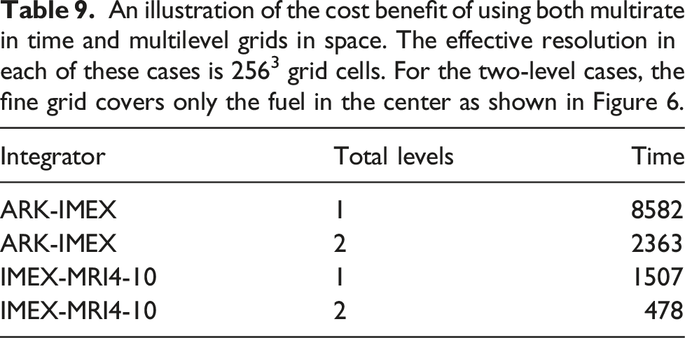
To demonstrate the advantage of using both multirate time stepping and multi-level grids, versus with or without either option alone, we ran both ARK-IMEX and IMEX-MRI4-10 on single- and two-level grids. In the multilevel case, the fine grid only covers the fuel in the center, that is, for a radius of 0.01 cm extending from the center of the domain (which covers [−0.05, 0.05] per side). In the single-level case, the domain contains 256³ grid cells divided into blocks of 32 cells on a side. In the multilevel case, we use an effective 256³ resolution with a coarse domain containing 128³ grid cells using blocks of 16 cells on a side to maintain the same number of MPI ranks as the single-level case, along with another level of refinement. A multilevel setup of our simulation is shown in Figure 6; we note that the fine grids cover roughly 5% of the domain volume. In the figure, the resolution is lower for clarity. We leverage the composite multilevel MLABecLaplacian operator built into AMReX for implicit diffusion. The solver tolerance is 10⁻¹² for all cases.

Table 9 shows that using either AMR or multirate alone takes considerably less time than single-rate time stepping on the single-level grid. However, combining the two techniques results in a considerably more efficient result than with either feature alone.

Table 9.

An illustration of the cost benefit of using both multirate in time and multilevel grids in space. The effective resolution in each of these cases is 256³ grid cells. For the two-level cases, the fine grid covers only the fuel in the center as shown in Figure 6.

Integrator	Total levels	Time
ARK-IMEX	1	8582
ARK-IMEX	2	2363
IMEX-MRI4-10	1	1507
IMEX-MRI4-10	2	478

7. Conclusions

With the continued increases in compute power delivered by high-performance systems, there continues to be increasing complexity in scientific simulations. One area where this complexity manifests is in modeling systems with more physical processes that may operate at differing temporal and spatial scales. Recent work in time integration methods has resulted in several new approaches to handling multiphysics systems with disparate time scales, and many of these are being developed into very efficient implementations within numerical libraries. In the meantime, work in mesh refinement technologies has resulted in highly efficient libraries for handling multiphysics systems with differing spatial scales. In this work, we evaluated new MRI and IMEX-MRI multirate time integration methods implemented within the SUNDIALS time integration library, along with block-structured spatial mesh discretization approaches implemented within the BoxLib and AMReX libraries. These evaluations were done within the context of high-performance computing systems and also included comparison with spectral deferred correction methods and their multirate variants. Results on two multiphysics test problems from combustion show that the new multirate methods match the accuracy of SDC and MRSDC methods while giving higher efficiency in most accuracy regimes. In addition, results show that the multirate methods are more efficient than single-rate methods for multiphysics systems posed within block-structured mesh frameworks. Lastly, the multirate and multi-spatial grid methods were shown to both improve overall solution efficiency, and their impacts were amplified when both approaches were simultaneously applied.

We expect these results to translate to other multiphysics systems with well separated time scales, such as those found in low Mach combustion systems and even in watershed models. In low Mach combustion, large time steps allow advection to be treated on a very slow time scale with implicit diffusion; reactions are even more challenging due to the wider separation of scales. In watershed systems, hydrological models must be advanced with significantly larger time steps than land models. Future work will consider application of multirate time integration methods to these and other applications.

Lastly, we note that the multirate methods can be made even more efficient through application of adaptive time step technologies that can additionally relieve users from manual discovery of appropriate fast and slow step sizes for their applications. These approaches have been very effective in single-rate methods. Current work is exploring how to bring such adaptivity into the multirate case.

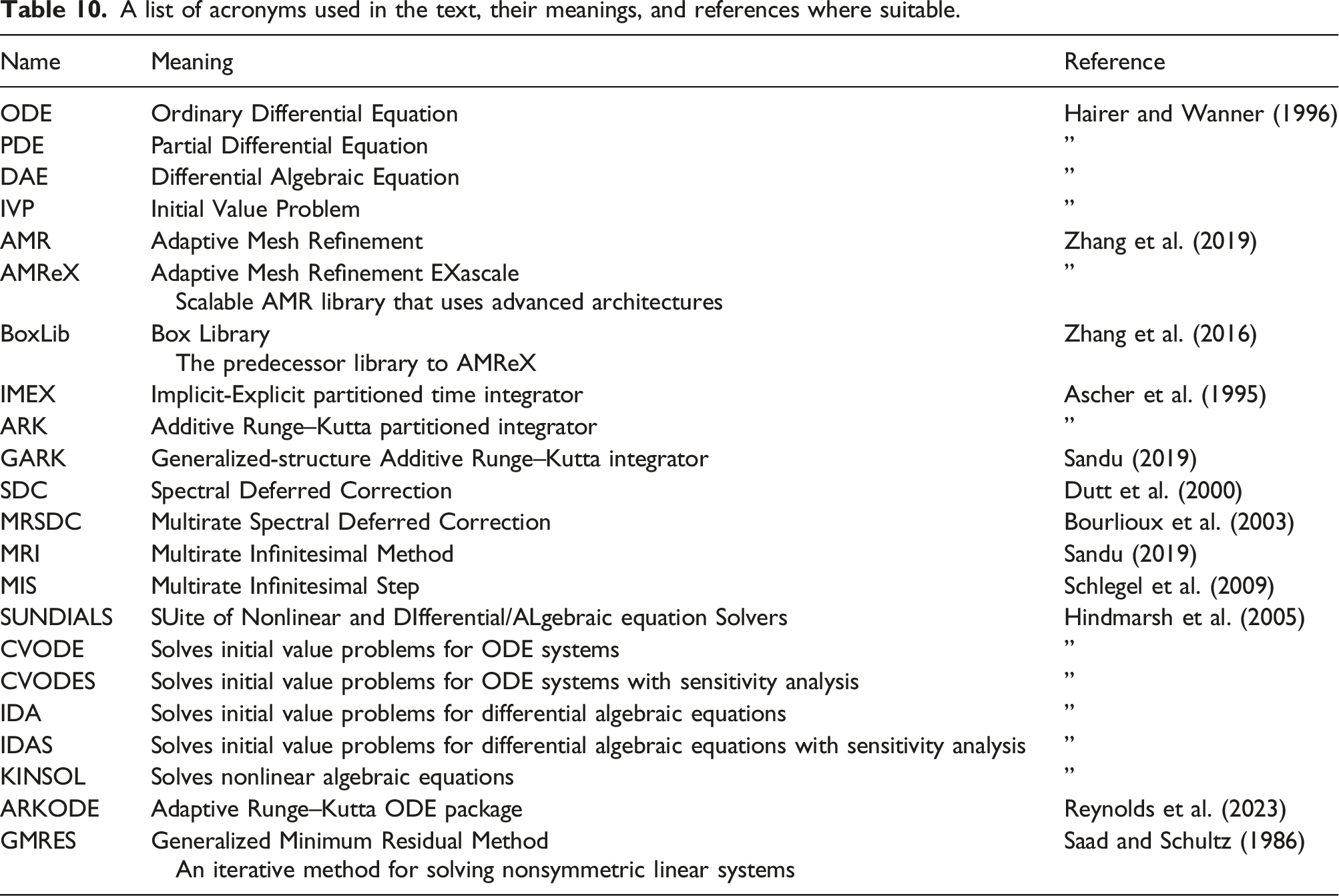
8. Description of acronyms and names

This manuscript includes a large number of acronyms. Table 10 provides a list of these acronyms, their meanings, and references where suitable.

Table 10.

A list of acronyms used in the text, their meanings, and references where suitable.

Name	Meaning	Reference
ODE	Ordinary Differential Equation	Hairer and Wanner (1996)
PDE	Partial Differential Equation	”
DAE	Differential Algebraic Equation	”
IVP	Initial Value Problem	”
AMR	Adaptive Mesh Refinement	Zhang et al. (2019)
AMReX	Adaptive Mesh Refinement EXascale	”
AMReX	Scalable AMR library that uses advanced architectures	”
BoxLib	Box Library	Zhang et al. (2016)
BoxLib	The predecessor library to AMReX	Zhang et al. (2016)
IMEX	Implicit-Explicit partitioned time integrator	Ascher et al. (1995)
ARK	Additive Runge–Kutta partitioned integrator	”
GARK	Generalized-structure Additive Runge–Kutta integrator	Sandu (2019)
SDC	Spectral Deferred Correction	Dutt et al. (2000)
MRSDC	Multirate Spectral Deferred Correction	Bourlioux et al. (2003)
MRI	Multirate Infinitesimal Method	Sandu (2019)
MIS	Multirate Infinitesimal Step	Schlegel et al. (2009)
SUNDIALS	SUite of Nonlinear and DIfferential/ALgebraic equation Solvers	Hindmarsh et al. (2005)
CVODE	Solves initial value problems for ODE systems	”
CVODES	Solves initial value problems for ODE systems with sensitivity analysis	”
IDA	Solves initial value problems for differential algebraic equations	”
IDAS	Solves initial value problems for differential algebraic equations with sensitivity analysis	”
KINSOL	Solves nonlinear algebraic equations	”
ARKODE	Adaptive Runge–Kutta ODE package	Reynolds et al. (2023)
GMRES	Generalized Minimum Residual Method	Saad and Schultz (1986)
GMRES	An iterative method for solving nonsymmetric linear systems	Saad and Schultz (1986)

Footnotes

Acknowledgements

This document was prepared as an account of work sponsored by an agency of the United States government. Neither the United States government nor Lawrence Livermore National Security, LLC, nor any of their employees makes any warranty, expressed or implied, or assumes any legal liability or responsibility for the accuracy, completeness, or usefulness of any information, apparatus, product, or process disclosed, or represents that its use would not infringe privately owned rights. Reference herein to any specific commercial product, process, or service by trade name, trademark, manufacturer, or otherwise does not necessarily constitute or imply its endorsement, recommendation, or favoring by the United States government or Lawrence Livermore National Security, LLC. The views and opinions of the authors expressed herein do not necessarily state or reflect those of the United States government or Lawrence Livermore National Security, LLC, and shall not be used for advertising or product endorsement purposes.

Declaration of conflicting interests

The author(s) declared no potential conflicts of interest with respect to the research, authorship, and/or publication of this article.

Funding

The author(s) disclosed receipt of the following financial support for the research, authorship, and/or publication of this article: This work was supported by the U.S. Department of Energy’s (DOE) Office of Advanced Scientific Computing Research (ASCR) via the Scientific Discovery through Advanced Computing (SciDAC) program at the FASTMath Institute. Work at LLNL was performed under the auspices of the U.S. Department of Energy by Lawrence Livermore National Laboratory under contract DE-AC52-07NA27344, Lawrence Livermore National Security, LLC. Work at LBL was performed under the auspices of the U.S. Department of Energy by the Lawrence Berkeley National Laboratory under contract DE-AC02-05CH11231.

ORCID iDs

John J. Loffeld

Andy Nonaka

Daniel R. Reynolds

David J. Gardner

Carol S. Woodward

Author biographies

John J. Loffeld has been at Lawrence Livermore National Lab since 2013, first as a postdoctoral researcher and then as a member of technical staff. At LLNL, he has worked on high-order finite-volume discretization, time integration, and methods for deterministic transport. He received a PhD in Applied Mathematics from the University of California at Merced in 2013 and a BA in Computer Science from the University of California at Berkeley in 1997. In the interim, he worked at Lawrence Berkeley National Lab as a software engineer.

Andy Nonaka is a Staff Scientist and Group Lead of the Center for Computational Sciences and Engineering at Lawrence Berkeley National Laboratory. He is interested in multiphysics PDE modeling and simulation on HPC systems using structured adaptive mesh, particle mesh, and machine learning algorithms. He works on applications including combustion, electrodynamics for microelectronics, stochastic PDEs for mesoscale flow, complex fluids, astrophysics, and general compressible, incompressible, and low Mach number fluid problems.

Daniel R. Reynolds is Professor and Chair of the Department of Mathematics at Southern Methodist University. His research focuses on the development and application of robust time integrators and iterative nonlinear and linear solvers for large-scale multiphysics systems—simulations comprised of multiple interacting physical processes. Reynolds is the creator of the ARKODE library, a collection of solvers for adaptive implicit-explicit and multirate time integration methods for large-scale systems of differential equations, and he is a senior developer for the larger SUNDIALS suite of time integration and nonlinear solver libraries (which includes ARKODE). Prior to joining SMU in 2008, Reynolds held postdoctoral research positions in the Department of Mathematics and the Center for Astrophysics and Space Sciences at the University of California, San Diego, and in the Center for Applied Scientific Computing at Lawrence Livermore National Laboratory. He received a PhD in Computational and Applied Mathematics from Rice University in 2003 and a BA in Mathematics from Southwestern University in 1998.

David J. Gardner is a computational scientist in the Center for Applied Scientific Computing at Lawrence Livermore National Laboratory. His research interests include the development, implementation, and deployment of accurate and efficient time integration methods and nonlinear solvers for simulating multiscale and multiphysics applications on high-performance computing systems. Gardner is a core developer of the SUNDIALS software library and has worked with scientific teams in a number of application areas including atmospheric dynamics, combustion, cosmology, additive manufacturing, quantum dynamics, and materials science. He joined CASC in 2014 after completing his PhD in computational and applied mathematics at Southern Methodist University that same year.

Carol S. Woodward is a Distinguished Member of the Technical Staff in the Center for Applied Scientific Computing at Lawrence Livermore National Laboratory (LLNL). Her research interests include iterative solvers for nonlinear and linear systems, time integration methods, and portable numerical software development. Woodward leads the SUNDIALS software library development and deployment team. She received a BS in mathematics from Louisiana State University and a PhD in computational and applied mathematics from Rice University. She has been at LLNL since 1996. She is a Fellow of the Society for Industrial and Applied Mathematics and the Association for Women in Mathematics.

References

Almgren

Bell

Lijewski

, et al. (2013) Nyx: a massively parallel amr code for computational cosmology. The Astrophysical Journal 765(1): 39. DOI: 10.1088/0004-637X/765/1/39.

Ascher

Ruuth

Wetton

BTR

(1995) Implicit-explicit methods for time-dependent partial differential equations. SIAM Journal on Numerical Analysis 32(3): 797–823. DOI: 10.1137/0732037.

Balos

Gardner

Woodward

, et al. (2021) Enabling GPU accelerated computing in the SUNDIALS time integration library. Parallel Computing 108: 102836. DOI: 10.1137/0732037.

Bartlett

Demeshko

Gamblin

, et al. (2017) xSDK Foundations: Toward an Extreme-scale Scientific Software Development Kit. Supercomputing Frontiers and Innovations 4(1): 69–82. DOI: 10.14529/jsfi170104.

Berger

Rigoutsos

(1991) An algorithm for point clustering and grid generation. IEEE Transactions on Systems, Man, and Cybernetics 21(5): 1278–1286. DOI: 10.1109/21.120081.

Bogacki

Shampine

(1989) A 3 (2) pair of Runge–Kutta formulas. Applied Mathematics Letters 2(4): 321–325. DOI: 10.1016/0893-9659(89)90079-7.

Bourlioux

Layton

Minion

(2003) High-order multi-implicit spectral deferred correction methods for problems of reactive flow. Journal of Computational Physics 189(2): 651–675. DOI: 10.1016/S0021-9991(03)00251-1.

Cash

Karp

(1990) A variable order Runge–Kutta method for initial value problems with rapidly varying right-hand sides. ACM Transactions on Mathematical Software 16(3): 201–222. DOI: 10.1145/79505.79507.

Cervi

Spiteri

(2019) A comparison of fourth-order operator splitting methods for cardiac simulations. Applied Numerical Mathematics 145: 227–235. DOI: 10.1016/j.apnum.2019.06.002.

10.

Chen

Choudhary

De Supinski

, et al. (2009) Terascale direct numerical simulations of turbulent combustion using s3d. Computational Science & Discovery 2(1): 015001. DOI: 10.1088/1749-4699/2/1/015001.

11.

Chinomona

Reynolds

(2021) Implicit-explicit multirate infinitesimal GARK methods. SIAM Journal on Scientific Computing 43(5): A3082–A3113. DOI: 10.1137/20M1354349.

12.

Day

Bell

(2000) Numerical simulation of laminar reacting flows with complex chemistry. Combustion Theory and Modelling 4(4): 535–556. DOI: 10.1088/1364-7830/4/4/309.

13.

Dutt

Greengard

Rokhlin

(2000) Spectral deferred correction methods for ordinary differential equations. BIT Numerical Mathematics 40(2): 241–266. DOI: 10.1023/A:1022338906936.

14.

Emmett

Zhang

Bell

(2014) High-order algorithms for compressible reacting flow with complex chemistry. Combustion Theory and Modelling 18(3): 361–387. DOI: 10.1080/13647830.2014.919410.

15.

Emmett

Motheau

Zhang

, et al. (2019) A fourth-order adaptive mesh refinement algorithm for the multicomponent, reacting compressible Navier–Stokes equations. Combustion Theory and Modelling 23(4): 592–625. DOI: 10.1080/13647830.2019.1566574.

16.

Estep

Ginting

Ropp

, et al. (2008) An a posteriori-a priori analysis of multiscale operator splitting. SIAM Journal on Numerical Analysis 46(3): 1116–1146. DOI: 10.1137/07068237X.

17.

Fan

Nonaka

Almgren

, et al. (2019) Maestroex: a massively parallel low mach number astrophysical solver. The Astrophysical Journal 887(2): 212. DOI: 10.3847/1538-4357/ab4f75.

18.

Frenklach

Wang

Goldenberg

, et al. (1995) Gri-mech—An Optimized Detailed Chemical Reaction Mechanism for Methane Combustion. Lawrence, KS: National Technical Reports Library. Gas Research Institute Topical Report No. GRI-95/0058.

19.

Gardner

Reynolds

Woodward

, et al. (2022) Enabling new flexibility in the SUNDIALS suite of nonlinear and differential/algebraic equation solvers. ACM Transactions on Mathematical Software 48(3): 1–24. DOI: 10.1145/3539801.

20.

Gear

Wells

(1984) Multirate linear multistep methods. BIT Numerical Mathematics 24(4): 484–502. DOI: 10.1007/BF01934907.

21.

Goldman

Kaper

(1996) N th-order operator splitting schemes and nonreversible systems. SIAM Journal on Numerical Analysis 33(1): 349–367. DOI: 10.1137/0733018.

22.

Günther

Sandu

(2016) Multirate generalized additive Runge–Kutta methods. Numerische Mathematik 133(3): 497–524. DOI: 10.1007/s00211-015-0756-z.

23.

Hairer

Wanner

(1996) Solving Ordinary Differential Equations II. New York: Springer Berlin Heidelberg, Vol. 375.

24.

Hindmarsh

Brown

Grant

, et al. (2005) SUNDIALS: suite of nonlinear and differential/algebraic equation solvers. ACM Transactions on Mathematical Software 31(3): 363–396. DOI: 10.1145/1089014.1089020.

25.

Huang

Pazner

Persson

, et al. (2020) High-order partitioned spectral deferred correction solvers for multiphysics problems. Journal of Computational Physics 412: 109441. DOI: 10.1016/j.jcp.2020.109441.

26.

Kee

Grcar

Miller

, et al. (1998) Premix Users Manual. San Diego, CA: Reaction Design.

27.

Kennedy

Carpenter

(2003) Additive Runge–Kutta schemes for convection–diffusion–reaction equations. Applied Numerical Mathematics 44(1–2): 139–181. DOI: 10.1016/S0168-9274(02)00138-1.

28.

Kennedy

Carpenter

Lewis

(2000) Low-storage, explicit Runge–Kutta schemes for the compressible Navier–Stokes equations. Applied Numerical Mathematics 35(3): 177–219. DOI: 10.1016/S0168-9274(99)00141-5.

29.

Knoll

Chacon

Margolin

, et al. (2003) On balanced approximations for time integration of multiple time scale systems. Journal of Computational Physics 185(2): 583–611. DOI: 10.1016/S0021-9991(03)00008-1.

30.

Knoth

Wolke

(1998) Implicit-explicit Runge–Kutta methods for computing atmospheric reactive flows. Applied Numerical Mathematics 28(2–4): 327–341. DOI: 10.1016/S0168-9274(98)00051-8.

31.

Kutta

(1901) Beitrag zur näherungsweisen integration totaler differentialgleichungen. Zeitschrift für Mathematik und Physik 46: 435–453.

32.

Layton

Minion

(2004) Conservative multi-implicit spectral deferred correction methods for reacting gas dynamics. Journal of Computational Physics 194(2): 697–715. DOI: 10.1016/j.jcp.2003.09.010.

33.

Luan

Chinomona

Reynolds

(2020) A new class of high-order methods for multirate differential equations. SIAM Journal on Scientific Computing 42(2): A1245–A1268. DOI: 10.1137/19M125621X.

34.

Marchuk

(1968) Some application of splitting-up methods to the solution of mathematical physics problems. Aplikace Matematiky 13(2): 103–132.

35.

McLachlan

Quispel

GRW

(2002) Splitting methods. Acta Numerica 11: 341–434. DOI: 10.1017/S0962492902000053.

36.

Minion

(2003) Semi-implicit spectral deferred correction methods for ordinary differential equations. Communications in Mathematical Sciences 1(3): 471–500.

37.

Nonaka

Bell

Day

, et al. (2012) A deferred correction coupling strategy for low mach number flow with complex chemistry. Combustion Theory and Modelling 16(6): 1053–1088. DOI: 10.1080/13647830.2012.701019.

38.

Nonaka

Day

Bell

(2018) A conservative, thermodynamically consistent numerical approach for low mach number combustion. part I: single-level integration. Combustion Theory and Modelling 22(1): 156–184. DOI: 10.1080/13647830.2017.1390610.

39.

Pazner

Nonaka

Bell

, et al. (2016) A high-order spectral deferred correction strategy for low mach number flow with complex chemistry. Combustion Theory and Modelling 20(3): 521–547. DOI: 10.1080/13647830.2016.1150519.

40.

Reynolds

Gardner

Woodward

, et al. (2023) Arkode: a flexible ivp solver infrastructure for one-step methods. ACM Transactions on Mathematical Software 49(2): 1–26. DOI: 10.1145/3594632.

41.

Roberts

Loffeld

Sarshar

, et al. (2021) Implicit multirate GARK methods. Journal of Scientific Computing 87(1): 1–32. DOI: 10.1007/s10915-020-01400-z.

42.

Saad

Schultz

(1986) Gmres: a generalized minimal residual algorithm for solving nonsymmetric linear systems. SIAM Journal on Scientific and Statistical Computing 7(3): 856–869. DOI: 10.1137/0907058.

43.

Sand

Skelboe

(1992) Stability of backward euler multirate methods and convergence of waveform relaxation. BIT Numerical Mathematics 32(2): 350–366. DOI: 10.1007/BF01994887.

44.

Sandu

(2019) A class of multirate infinitesimal GARK methods. SIAM Journal on Numerical Analysis 57(5): 2300–2327. DOI: 10.1137/18M1205492.

45.

Schlegel

(2011) A Class of General Splitting Methods for Air Pollution Models: Theory and Practical Aspects. PhD Thesis. Halle, Germany: Martin Luther University Halle-Wittenbergk.

46.

Schlegel

Knoth

Arnold

, et al. (2009) Multirate Runge–Kutta schemes for advection equations. Journal of Computational and Applied Mathematics 226(2): 345–357. DOI: 10.1016/j.cam.2008.08.009.

47.

Sexton

Lukic

Almgren

, et al. (2021) Nyx: a massively parallel amr code for computational cosmology. Journal of Open Source Software 6(63): 3068. DOI: 10.21105/joss.03068.

48.

Strang

(1968) On the construction and comparison of difference schemes. SIAM Journal on Numerical Analysis 5(3): 506–517. DOI: 10.1137/0705041.

49.

Vay

Almgren

Bell

, et al. (2018) Warp-x: a new exascale computing platform for beam–plasma simulations. Nuclear Instruments and Methods in Physics Research Section A: Accelerators, Spectrometers, Detectors and Associated Equipment 909: 476–479. DOI: 10.1016/j.nima.2018.01.035.

50.

Wartha

Bösenhofer

Harasek

(2020) Characteristic chemical time scales for reactive flow modeling. Combustion Science and Technology 193: 2807–2832. DOI: 10.1080/00102202.2020.1760257.

51.

Zhang

Almgren

Day

, et al. (2016) Boxlib with tiling: an adaptive mesh refinement software framework. SIAM Journal on Scientific Computing 38(5): S156–S172. DOI: 10.1137/15M102616X.

52.

Zhang

Almgren

Beckner

, et al. (2019) AMReX: a framework for block-structured adaptive mesh refinement. Journal of Open Source Software 4(37): 1370–1370. DOI: 10.21105/joss.01370.

53.

Zhang

Myers

Gott

, et al. (2021) Amrex: block-structured adaptive mesh refinement for multiphysics applications. The International Journal of High Performance Computing Applications 35(6): 508–526. DOI: 10.1177/10943420211022811.

54.

Zingale

Katz

Bell

, et al. (2019) Improved coupling of hydrodynamics and nuclear reactions via spectral deferred corrections. The Astrophysical Journal 886(2): 105. DOI: 10.3847/1538-4357/ab4e1d.

55.

Zonneveld

(1963) Automatic Integration of Ordinary Differential Equations. Amsterdam: Stichting Mathematisch Centrum. Technical Report 743.

Performance of explicit and IMEX MRI multirate methods on complex reactive flow problems within modern parallel adaptive structured grid frameworks

Abstract

Keywords

1. Introduction

2. Multirate time integration

2.1. IMEX-MRI-GARK

2.2. Multirate SDC methods

3. Model equations

3.1. Spatial discretization

3.2. Temporal discretization

4. Implementation

4.1. Block-structured meshes

4.2. Time integrators

5. Explicit time stepping on compressible reacting flow

5.1. Problem setup

5.2. Results

6. IMEX time stepping on a reacting flow problem implemented in AMReX

6.1. Problem setup

6.2. Results

6.3. Simulation on multilevel grids

7. Conclusions

8. Description of acronyms and names

Footnotes

Acknowledgements

Declaration of conflicting interests

Funding

ORCID iDs

Author biographies

References