Experiences with nested parallelism in task-parallel applications using malleable BLAS on multicore processors

Abstract

Malleability is defined as the ability to vary the degree of parallelism at runtime, and is regarded as a means to improve core occupation on state-of-the-art multicore processors tshat contain tens of computational cores per socket. This property is especially interesting for applications consisting of irregular workloads and/or divergent executions paths. The integration of malleability in high-performance instances of the Basic Linear Algebra Subprograms (BLAS) is currently nonexistent, and, in consequence, applications relying on these computational kernels cannot benefit from this capability. In response to this scenario, in this paper we demonstrate that significant performance benefits can be gathered via the exploitation of malleability in a framework designed to implement portable and high-performance BLAS-like operations. For this purpose, we integrate malleability within the BLIS library, and provide an experimental evaluation of the result on three different practical use cases.

Introduction

Task-level malleability is a well-appreciated property in cloud computing, where it refers to the capability of expanding/shrinking the number of resources allocated to a certain job during its execution. Process-level malleability can also offer significant performance benefits for distributed MPI scientific applications though, in that context, it is considerably more challenging due to the necessary re-distribution of the workload and data; see Iserte et al. (2017), Iserte et al. (2018) and the references therein.

In contrast, the concept of exploiting thread-level malleability inside an application may seem simple, both when using POSIX threads (pthreads) or a high level parallel application programming interface (API) such as OpenMP (OpenMP Architecture Review Board, 2018), but there are still relevant challenges that must be addressed to demonstrate its benefits. In particular, many applications rely on Linear Algebra threaded libraries (TLs), such as the Level-3 Basic Linear Algebra Subprograms (BLAS) (Dongarra et al., 1990), which are internally parallelized to optimize performance on multicore processors (Intel, 2020; OpenBLAS, 2015; Van Zee and van de Geijn, 2015).

TLs can exhibit three different degrees of flexibility to determine the number of threads that execute a specific kernel:

• Static TLs, in which the number of threads is decided at the program level, and hence it cannot vary throughout the execution of the complete program. Therefore, the number of threads is constant across all kernels within the execution.

• Moldable TLs, in which the number of threads executing a kernel can be varied dynamically across different kernels, but in all cases before the execution of each individual kernel starts.

• Malleable TLs, in which the number of threads executing a kernel can vary dynamically and upon request while the kernel is under execution. Currently, the support for malleability in TLs is scarce or non-existent on both commercial and open-source TLs.

Additionally, applications where each task basically requires the execution of a kernel from a linear algebra library can exploit parallelism either (1) from within the application only, (2) from inside the library kernels only, or (3) a combination of both (that is, application + library) (Dolz et al., 2015). In this paper, we revisit the third approach, exploring the performance benefits of composing a task-parallel Application (TA) with a thread-level malleable BLAS (MLB). Concretely, our TA + MLB approach divides the existing threads into t _App teams, handled by the application, where each team (comprising one or more threads) is in charge of executing a single task/linear algebra kernel. Alluringly, in our TA + MLB approach, the number of threads in each team cannot only vary dynamically during the timespan of the application, but also during the execution of each individual linear algebra kernel.

Our dynamic approach at the kernel level is built on top of an instance of MLB developed using the Basic Linear Algebra Instantiation Software (BLIS) (Van Zee and Van de Geijn, 2015). In Catalán et al. (2019, 2020) this solution was reported to deliver considerable benefits for the execution of the (dense) LU factorization on current multicore processors in comparison with classical solutions that exploit parallelism only within the BLAS (as, for example, is done when combining the legacy LAPACK with a multi-threaded realization of BLAS) as well as more modern realizations of this factorization, via a rutime, that exploit parallelism only at the task/application level (Buttari et al., 2009; Quintana-Ortí et al., 2009; Badia et al., 2009).

In this paper we progress a significant step forward toward demonstrating the benefits of the TA + MLB approach via the elaboration and analysis of a collection of three cases beyond the simple LU matrix decomposition. In particular, we develop TA + MLB implementations of the following case studies, investigating different parallelization strategies, gaining insight on applicability/advantages, and reporting the performance of this approach:

– QR factorization for the solution of (full rank) linear least squares problems (Golub and Loan, 1996).

– Matrix inversion via Gauss-Jordan elimination (Householder, 1964).

– Inference with deep neural networks (Sze et al., 2017).

The rest of the paper is structured as follows. After a general overview of the mechanisms to exploit parallelism in task-parallel applications, we then assess the benefits obtained from the introduction of the malleability mechanism in dense algebra applications and deep learning. We close the paper with some concluding remarks and proposal for other applications of malleability.

Exploiting parallelism in task-parallel applications

Let us consider an application composed of a collection of tasks, intertwined via task dependencies, and where each task basically requires the execution of a kernel from a linear algebra library (e.g., BLAS). The left-hand side panel in Figure 1 displays a simple workhorse example for the following discussion, consisting of four tasks, numbered as T0–T3, with data dependencies T0 → T1 → T3 and T0 → T2 → T3. The height of each box depicted there is meant to be proportional to the cost of the task (indicated by the value inside the parenthesis). In this simple case, each task involves the execution of a single linear algebra kernel.

Figure 1.

Task-parallel application and parallelization schemes. SA + TL and TA + TL(1) use static TLs; TA + TL(2) is an example of the application of moldable TLs; TA + MLB requires a malleable TL.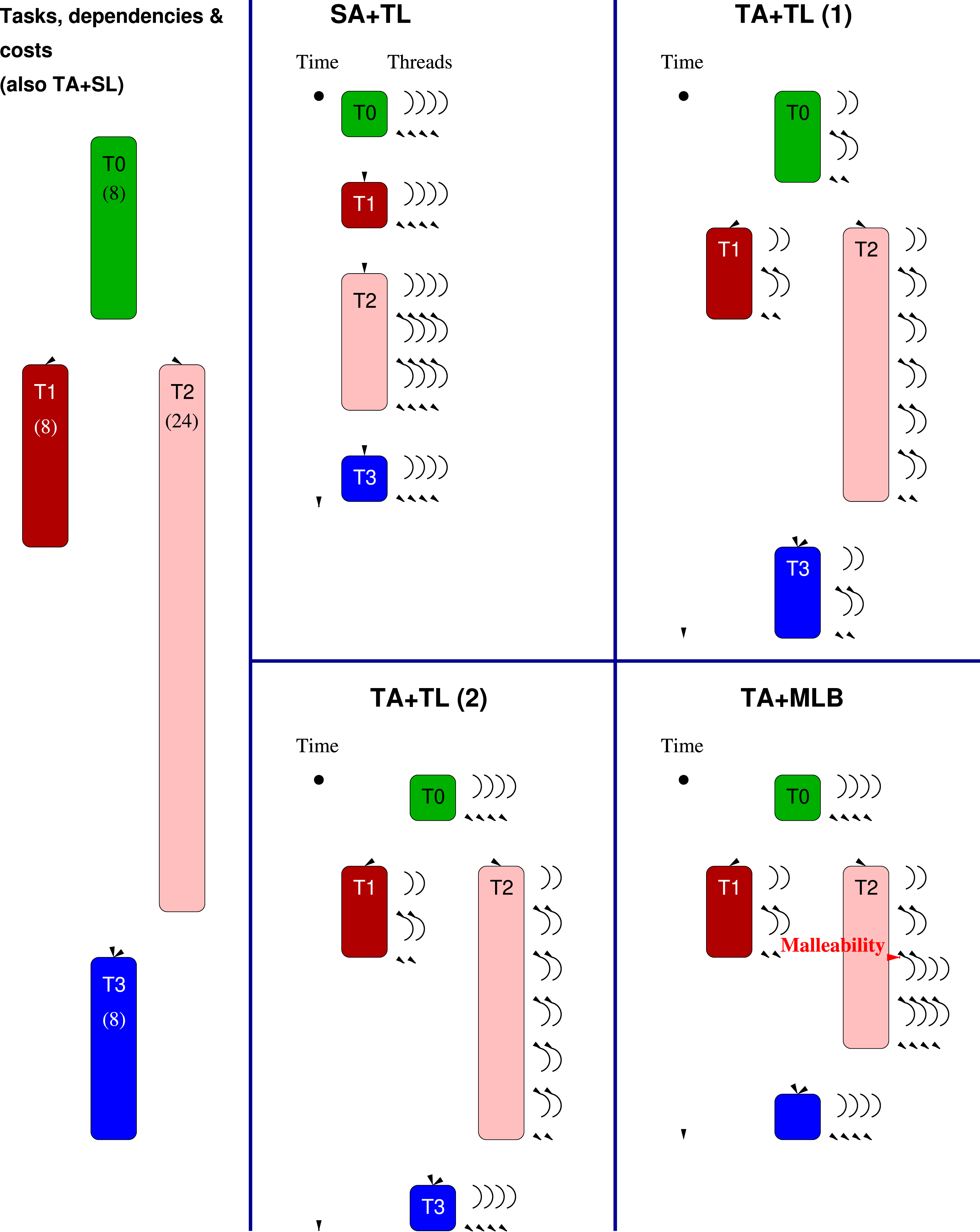

This type of application can be parallelized via one of the following three schemes, each presenting some advantages and caveats (Dolz et al., 2015):

• Sequential application invoking a threaded library ( SA + TL ). This option extracts the parallelism from inside the linear algebra kernels only, executing the tasks in sequential order (hence the name “sequential” application). That is, at any moment, there is only one task in execution, but the corresponding kernel can be processed using multiple threads via the call to a linear algebra TL. This is illustrated by the panel labelled as SA + TL in Figure 1. There we assume an ideal scenario where the kernels are embarrassingly parallel. Thus, the parallel execution of a task with a cost of c units of time, using t threads, reduces the execution time by a factor of t, i.e. the reduced execution time is c/t units of time.

      A performance pitfall appears for applications that involve, as part of their computation, a non-negligible number of sequential kernels, which cannot benefit from a multi-threaded execution. For example, this is the case when the sequential kernels present a high computational complexity since, with this scheme, their cost cannot be hidden by overlapping their execution with that of other (independent) kernels. In the simple example in Figure 1 this would occur, for example, if task T2 was mostly sequential, so that its execution using four threads would yield no reduction in the run time compared to a sequential execution.

• TA invoking a sequential library ( TA + SL ). This is often the preferred solution for TAs, where parallelism is extracted at the application level only, usually by a runtime that orchestrates a dependency-aware execution of the task graph, and with each task executed by invoking a kernel from a sequential (linear algebra) library. This case is implicitly represented in the leftmost panel of Figure 1, where each thread is executed by a single thread, respecting the task dependencies. Tasks T1 and T2 present no dependencies and, therefore, can proceed concurrently.

     A caveat of this scheme is that it requires decomposing the application into a “sufficient” number of tasks of the “appropriate” granularity, exposing a delicate balance:

– On the one hand, if the tasks are too coarse, there may be too few of them, limiting the parallel scalability (at the application level). Also, dividing the tasks into finer-grain sub-tasks can be infeasible for some applications.

– On the other hand, creating too many tasks increases the overhead introduced by the runtime in charge of controlling task dependencies. Furthermore, it may result in suboptimal execution of the sequential linear algebra kernels, which may be too small to properly exploit the memory hierarchy of the system (Low et al., 2014).

– Finally, for TAs comprising large, compute-intensive linear algebra kernels with few dependencies (such as those in the Level-3 BLAS), the TA + SL scheme in general renders lower performance than an alternative which simply combines a SA with a multi-threaded version of the BLAS (Catalán et al., 2019, 2020).

• TA invoking a threaded library ( TA + TL ). This is the scheme illustrated in the panel labelled as TA + TL (1) in Figure 1 where, as in the previous case, parallelism is extracted at the application level by a runtime.

However, each task is now executed using (a fixed number of) two threads. This case is an example of the use of a static TL, where the number of threads per task is defined on a per-application basis, and does not vary neither across kernel invocation nor inside kernels.

     This option should be adopted with care as it is prone to incur in thread over-subscription, (that is, creating more threads than physical cores) which, for task-parallel applications involving linear algebra kernels, often results in low performance on modern multi-core processors.

In this paper we revisit the TA + TL scheme, enhancing it with malleability in order to produce a more efficient solution. In particular, consider the execution graphically represented in the panel labelled as as TA + TL (2) in Figure 1. This obviously produces a more efficient schedule than its counterpart TA + TL (1), as the number of threads assigned to the execution of a task is not fixed but can take advantage of all the available resources at the beginning of the execution of a task. This is an example of a moldable TL, in which the number of threads is determined on a per-kernel basis. Unfortunately, this option still presents a performance penalty as, with current instances of BLAS, upon completion, the two threads that participated in the execution of task T1 must remain idle till the execution of task T2 is complete.

The approach proposed in this paper progresses one step further in the direction of malleability to allow that the number of threads that participate in the execution of a task varies during the execution of the corresponding linear algebra kernel. This is illustrated in the panel labelled as TA + MLB in Figure 1, where the two threads that were in charge of executing task T1 commence to collaborate in the execution of task T2 as soon as they are done with the former. This is an example of a malleable TL, in which the number of threads assigned to the execution of a specific kernel can be modified during its execution.

Our dynamic, kernel-level malleable scheme tackles the two following scheduling-related problems. Consider a task-parallel application to be executed by a runtime using a number of “application thread teams” T _A , T _B , T _C , …, with each application team in charge of executing a single task at any given moment. (For example, in the TA + TL (1) in Figure 1 there are two application teams, each consisting of two threads.) Assume the application team T _A is about to commence the execution of task/kernel T:

– The application team T _A could benefit from a larger number of threads than those currently allocated to it. However, its peer application teams T _B , T _C , … are currently executing other linear algebra kernels and, with existing non-malleable libraries, will not release their resources until they complete their job. Should application team T _A wait until this occurs or commence the execution of T right away? In the second case, the call to a non-malleable library implies that T _A cannot benefit from additional idle resources (i.e., threads), liberated by any peer application team, once its execution of kernel T has commenced.

– Assume that, for this kernel T, the application team T _A will not really gain much, in terms of performance, from using all threads currently assigned to it. However, if this application team T _A releases the unnecessary resources, these threads will remain idle until any other peer application team completes the execution of its corresponding kernel and can make use of them in the execution of a subsequent task. Ideally, we would prefer that T _A liberates the unnecessary threads, which then move to help other peer application teams with the execution of their jobs.

To avoid these problems, we adopt a dynamic solution, where the threads migrate between application teams on-the-fly, during the execution of the kernels, using a particular MLB built on top of BLIS (Van Zee and Van de Geijn, 2015). In the next few sections, we illustrate the benefits of this approach using three relevant cases from dense linear algebra and deep learning, running on multicore processor architectures.

Integrating malleability in BLIS

The malleability mechanism that we integrated into BLIS v0.5.1 is described in detail in Rodríguez-Sánchez et al. (2020) together with an analysis of the overhead introduced by this mechanism. For brevity, we only summarize next the most relevant aspects of this integration.

In order to introduce malleability the key is to leverage (and modify) the BLIS API to distinguish in the library between 1) the maximum number of threads and 2) the active number of threads. The former parameter specifies the amount of threads that are initially active when invoking a routine, and it typically matches the number of cores of the machine. The latter parameter specifies the number of threads that participate in a given computation at a specific time, and can be modified asynchronously at any time by any application thread.

Using these two parameters, the workload for each of the nested loops (which corresponds to the iteration space for that loop) in the BLIS routine is distributed among the threads. As a result, those threads without any workload assigned to them in a given loop immediately proceed to the end of that loop, where they remain blocked (in a passive wait, to avoid wasting resources) till all the active threads that participate in the execution of that loop complete their part of the work.

Dense linear algebra

QR factorization with look-ahead

Algorithms Consider the QR factorization (Golub and Loan, 1996) of an m × n nonsingular matrix A, given by A = QR, where the m × m matrix Q is orthogonal and the m × n factor R is upper triangular. For simplicity, hereafter we assume that n is an integer multiple of the algorithmic block size b. Furthermore, we consider a column partitioning of A into s = n/b blocks, of b columns each. In our notation, A(:, c₁ : c₂) refers to the submatrix of A that spans the c₁, c₁ + 1, …, c₂-th panels (or column blocks) of A, comprising columns c₁ · b, c₁ · b + 1, …, c₂ · b − 1. (Note that, in our notation, the indices for blocks and elements start at 0.)

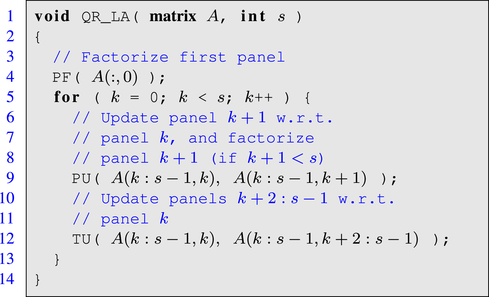
Listing 1 and the accompanying Figure 2 shows a (simplified version) of a blocked algorithm that computes the QR factorization of a square n × n matrix A expressed with a high level of abstraction. This formulation corresponds to a blocked algorithm that offers high performance provided b is moderately large, by reducing the ratio between flops and memory accesses. The algorithm performs s iterations, with the loop body first computing the factorization of the “current” panel (that is, the k-th column block); and then updating the panels to its right with the corresponding orthogonal transforms (trailing update). For simplicity, these two operations are encapsulated inside routines PF and TU, respectively. They are also quite different: PF is mostly a sequential operation while TU can be performed via highly parallel Level-3 BLAS.

Figure 2.

Partitioning of a matrix consisting of s × s blocks, with s = 5, and operations performed at iteration k = 1 of the algorithm for the QR factorization in Listing 1.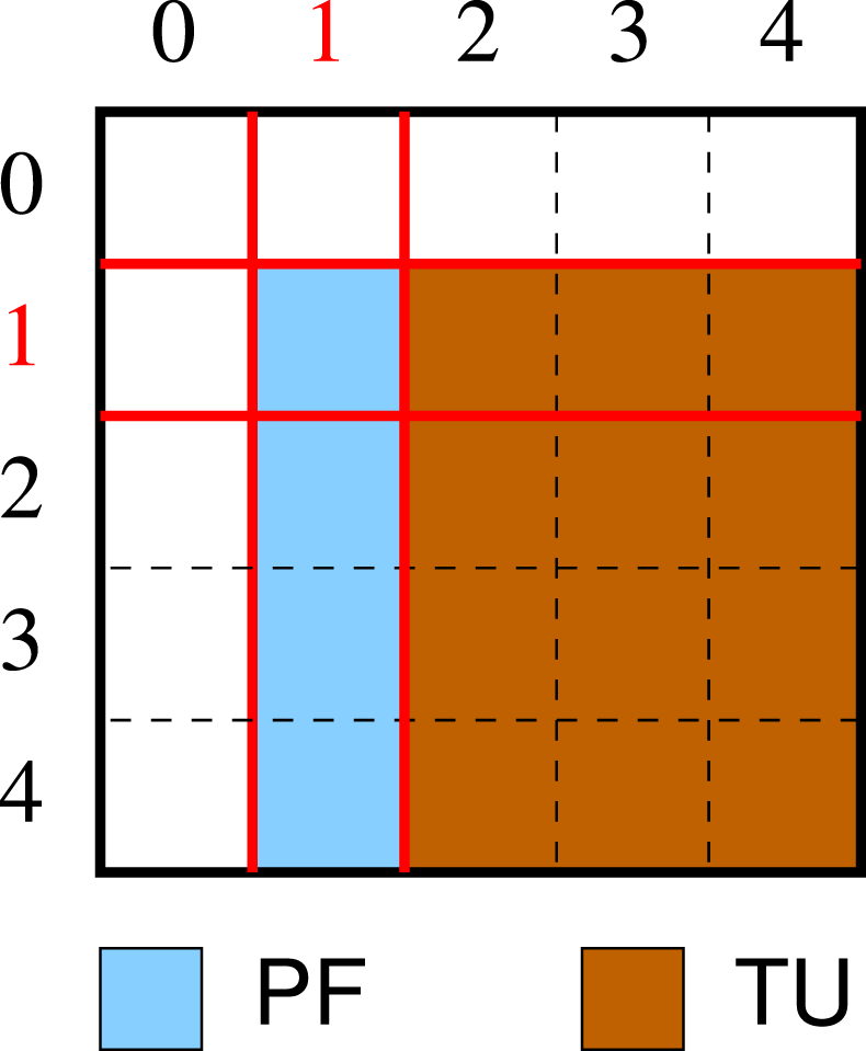

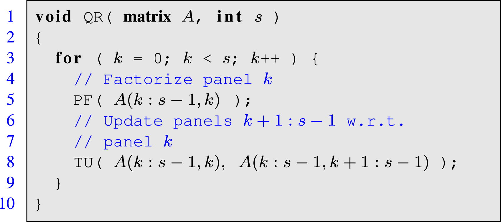
Listing 1: Simplified routine for the QR factorization.

The conventional approach to parallelize this matrix factorization is to exploit loop-parallelism from within the (Level-3) BLAS only, which corresponds to the SA + TL scheme. In the past decade, there has been a notable interest in exposing and leveraging task-parallelism at a higher level, from the LAPACK routines themselves, while relying on a sequential version of the BLAS, as corresponds to the TA + SL scheme; see, e.g., Buttari et al. (2009), Quintana-Ortí et al. (2009), and Badia et al. (2009). For the QR factorization, this is often performed by 1) dividing both PF and TU into finer-grain tasks; 2) leveraging a runtime to orchestrate a dependency-aware parallel schedule of these tasks; and 3) employing a sequential version of the BLAS to execute each individual task.

In our work, we follow an alternative nested-parallel TA + TL scheme that exploits task-parallelism at the factorization level (i.e., the application) and loop-parallelism within the invoked routines of BLAS (i.e., the “library”). For TAs comprising large, compute-intensive linear algebra kernels from BLAS, we have found that this approach offers competitive performance compared with the SA + TL and TA + SL schemes (Catalán et al., 2019, 2020).

In order to expose nested parallelism for the TA + TL scheme, we first need to reformulate the basic algorithm in Listing 1, in order to avoid the strict task dependencies between the two operations (tasks) that appear in the loop body. For this purpose, we consider a variant of this blocked algorithm enhanced with look-ahead (Strazdins, 1998), where an iteration of the loop body comprises the update of the trailing submatrix with respect to the current panel and the factorization of the “next” panel (k + 1-th column block). Concretely, the reformulated loop body for the QR factorization is shown in Listing 2.

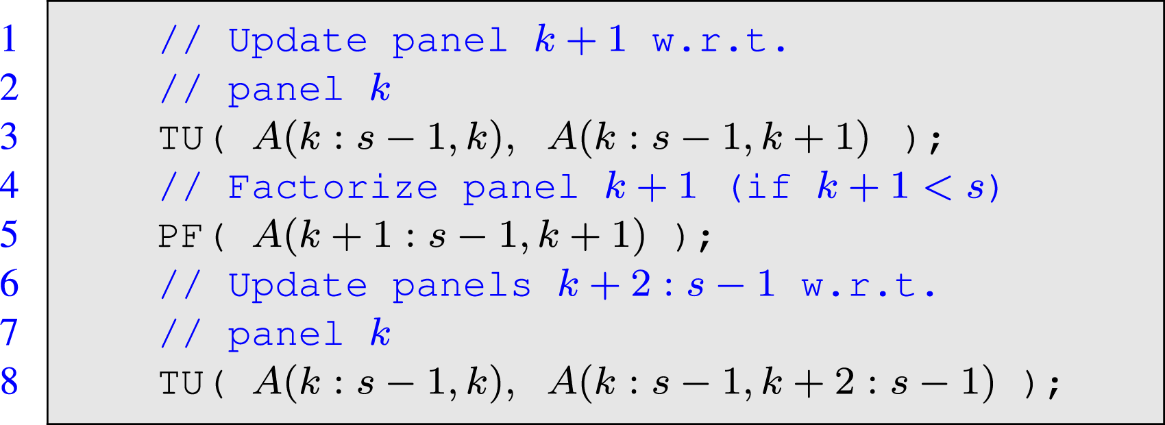
Listing 2: Reformulated QR factorization.

For simplicity, let us aggregate the update of the trailing (k + 1)-th panel and the subsequent factorization of the same panel in this code excerpt into a single operation, hereafter named panel update (and encapsulated inside PU). This results in the simplified algorithm for the QR factorization with look-ahead in Listing 3.

Listing 3: Simplified routine for the QR factorization with look-ahead.

Compared with the conventional algorithm for the QR factorization (that is, the realization without look-ahead in Listing 1), the variant with look-ahead features a loop body consisting also of two tasks: PU and TU, where the former is still mostly sequential while the latter can be performed via highly parallel Level-3 BLAS. However, in contrast with the standard algorithm, the two tasks in the loop body are now independent and, therefore, they can be executed in parallel. The main advantage of the look-ahead reformulation of the algorithm is that, because of the independence between the two operations in the loop body, it can overlap the execution of the small, sequential panel update with that of the large parallel trailing update. This is relevant since, as the number of cores grows, the panel update cannot take advantage of the increasing volume of hardware resources, and eventually becomes a performance bottleneck.

In order to exploit the task independence in the look-ahead variant via nested parallelism (TA + TL) we proceed as follows: We divide the threads into two application thread teams so that, at each iteration of the loop, team T _P is in charge of the execution of PU and team T _T of TU. In addition, to handle the different degrees of parallelism of the two tasks, we obviously assign many more threads to team T _T than to team T _P .

During the factorization, the ratio between the floating point operations (flops) performed inside the PU and TU vary, introducing two sources of workload imbalance:

W1. In case PU (which exhibits little parallelism) takes longer to execute than TU, team T _T will complete its work earlier than team T _P , and the (much larger amount of) threads assigned to the former team will remain idle till the beginning of the next iteration, wasting precious resources.

     To tackle this problem, we can apply an early termination mechanism (developed in Catalán et al. (2019) for the LU factorization) that quits the execution of PU (and delays the pending part of the panel factorization to the subsequent iteration) as soon as the team in charge of TU notifies it has completed its job. This is equivalent to a dynamic, adaptive tuning of the algorithmic block size b.

W2. At the other extreme, the cost of PU may be considerably smaller than that of TU, resulting in team T _P completing its execution earlier than its peer, again wasting resources.

     In the case, we leverage MLB to enforce that, as soon as the threads in team T _P are finished with PU, they join those in team T _T for the collaborative execution of TU.

In Catalán et al. (2020), we analyzed how to integrate task-parallelism with MLB, from the point of view of parallel programming. That work evaluated this solution for three matrix factorizations: LU (with partial pivoting), QR, and reduction to symmetric band form. However, the study performed there had a few relevant simplifications: 1) the team in charge of the panel factorization comprised a single thread only; 2) the solution did not include early termination; and 3) the malleability mechanism was not integrated into BLIS. In this paper we overcome these simplifications to offer a more complete experimental assessment of the benefits of nested TA + TL scheme.

Performance evaluation

The following experiments (and those in the second use case in this section) were carried out on a platform equipped with a 20-core Intel Xeon Gold 6138 processor (Skylake micro-architecture). The reference codes were compiled with icc version 18 and linked with OpenMP 4.5 and either BLIS v0.5.1 or MKL 2018.1.163, and the malleability mechanism was integrated into BLIS v0.5.1 (Rodríguez-Sánchez et al., 2020). All experiments were performed in double precision. In addition, in order to avoid the performance distortions caused by the aggressive utilization of the power modes (and associated frequencies) featured by Linux governor for the Intel® Xeon® Gold 6138 processor (Intel, 2019), the operating frequency for all cores was set to 1.7 GHz.

Figure 3 reports the performance of the following codes for the QR factorization of square (m = n) matrices:

– MKL. The multi-threaded implementation of this operation in Intel MKL. As this library offers a “black-box” solution, it is not possible to infer how parallelism is exploited from within the Intel realization.

– SQR + MKL/BLIS. C implementation of the LAPACK routine to calculate the QR factorization (routine dgeqrf) enhanced with some algorithmic optimizations (in particular, in the scheme to accumulate the orthogonal transforms (Joffrain et al., 2006)), and linked with multi-treaded (TL) instances of either Intel MKL or BLIS to execute the kernels invoked from within the LAPACK routine. The implementation exclusively relies on Level-3 BLAS kernels, i.e. no Level-1 and Level-2 BLAS kernels are instantiated. Note that this corresponds to a SA + TL scheme as the algorithm for the QR factorization is “sequential” but invokes BLAS kernels from a multithreaded linear algebra library.

– TQR + LA. A variant of the SQR implementation modified to encode look-ahead, with task parallelism exploited using OpenMP. This is the baseline version to obtain a TA + TL scheme.

– TQR + MLB. Same variant as TQR + LA, but linked with the malleable version of BLIS and enhanced with the early termination mechanism.

Figure 3.

Performance of the QR factorization.

TQR + LA and TQR + MLB are both realizations of TA + TL schemes. For these two options we evaluate three configurations, which split the threads into two teams, T _P + T _T , with the team in charge of the panel update comprising p = 1, 2 or 3 threads, and the remaining t − p threads dedicated to the trailing update. This is denoted in the plots for t = 12, 20 cores with the addition of a suffix of the form “p+(t-p)” to the line legend. For example, for the plot with 12 cores, the line labeled as “TQR + MLB 2 + 10” indicates the execution of variant TQR + MLB with two threads initially assigned to the panel update and 10 to the trailing update. Note that, being a malleable variant, the two threads in charge of the panel proceed to help with the update as soon as this task is completed. In all cases (except MKL, for which we have no control), the algorithmic block size was manually tuned to optimize performance and it is set to 384.

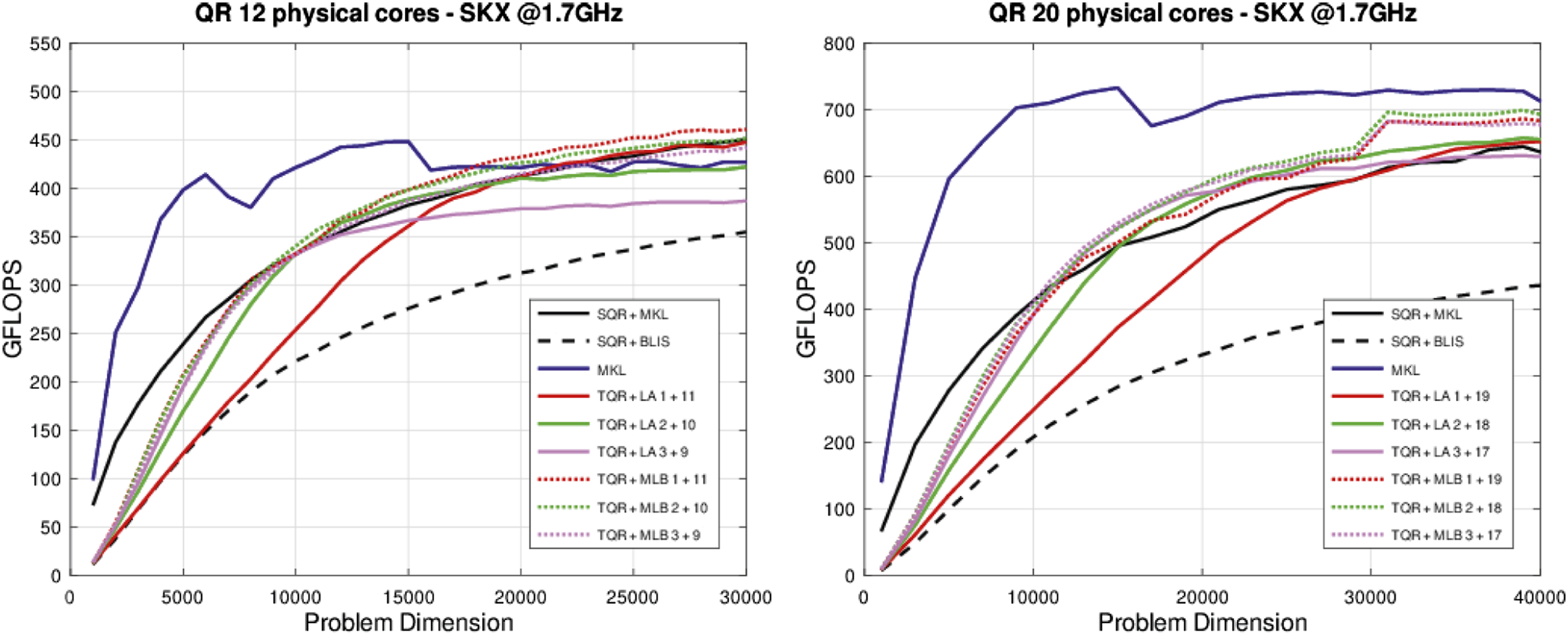
Figure 3 reports the results of the execution of the routines for the QR factorization using 12 and 20 cores (that is, the full socket in the latter case). Focusing on the SQR curves, the plots reveal that the version linked with Intel MKL outperforms that with BLIS by a large margin. The reason for this is that MKL is able to extract higher parallel performance than BLIS for certain gemm shapes (in particular, those involving very narrow panels) that mainly appear in PU. Fortunately, the introduction of the look-ahead mechanism (TQR + LA lines) partially hides this performance degradation for medium to large problem dimensions. In addition, for the TQR + LA scheme the best thread configuration greatly depends on the problem dimension. For small problems, PU may become a performance bottleneck and, therefore, it is necessary to devote more threads to its execution than for the large problem cases. In several independent experiments (not shown for brevity) we verified that the use of more than three threads to execute PU does not increase the performance of the global QR factorization procedure. For large problems, where PU is not a performance bottleneck and its execution cost is completely hidden with those of TU, we only need to employ one thread for PU. Regarding the TQR + MLB results, the plots reveal that the integration of maleability yields performance rates that are always superior to those of its counterparts that only leverage look-ahead. By adding this technique there appear no idle threads during the execution of the entire QR factorization, and as a consequence, the resources are more efficiently utilized. Finally, the approach proposed in this work outperforms the routine in MKL for the QR factorization for medium to large problems when 12 cores are used. Unfortunately, this behaviour is not observed for 20 cores because, with this configuration, the execution of PU becomes critical, and the baseline kernels in BLIS are not as efficient as those in MKL with the operand shapes that appear in this particular linear algebra operation.

Matrix inversion via GJE with look-ahead

Algorithms. The Gauss-Jordan elimination (GJE) can be leveraged to build a direct procedure to compute the matrix inverse (Householder, 1964) that offers remarkable efficiency on modern multicore and manycore architectures (Benner et al., 2013). Moreover, similarly to the classical multi-stage matrix inversion algorithm via the LU decomposition (Golub and Loan, 1996), the practical numerical stability of the GJE-based procedure can be ensured via the introduction of partial pivoting (Higham, 2002). For simplicity, we do not include pivoting in the following description of the inversion algorithms though all our practical implementations evaluated in this section include this technique.

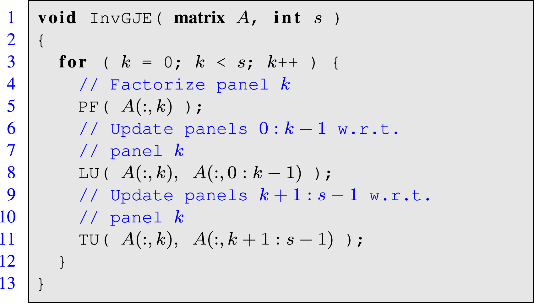
Listing 4: Simplified routine for matrix inversion via GJE.

Consider a nonsingular n × n matrix A. Listing 4 illustrates the procedure for matrix inversion via GJE adopted the same notation introduced for the presentation of the algorithms for the QR factorization. At each iteration of the loop in the blocked algorithm, indexed by k, the procedure first computes the “factorization” of the k-th (column) panel of the matrix. Once this panel is processed, via routine PF (for panel factorization), the inversion procedure updates the leading submatrix (panels) to its left via routine LU (for leading udpate); and the trailing submatrix (panels) to its right via routine TU (for trailing update). Here, the degree of parallelism of PF is scarce, while both LU and TU are composed of highly parallel matrix multiplications.

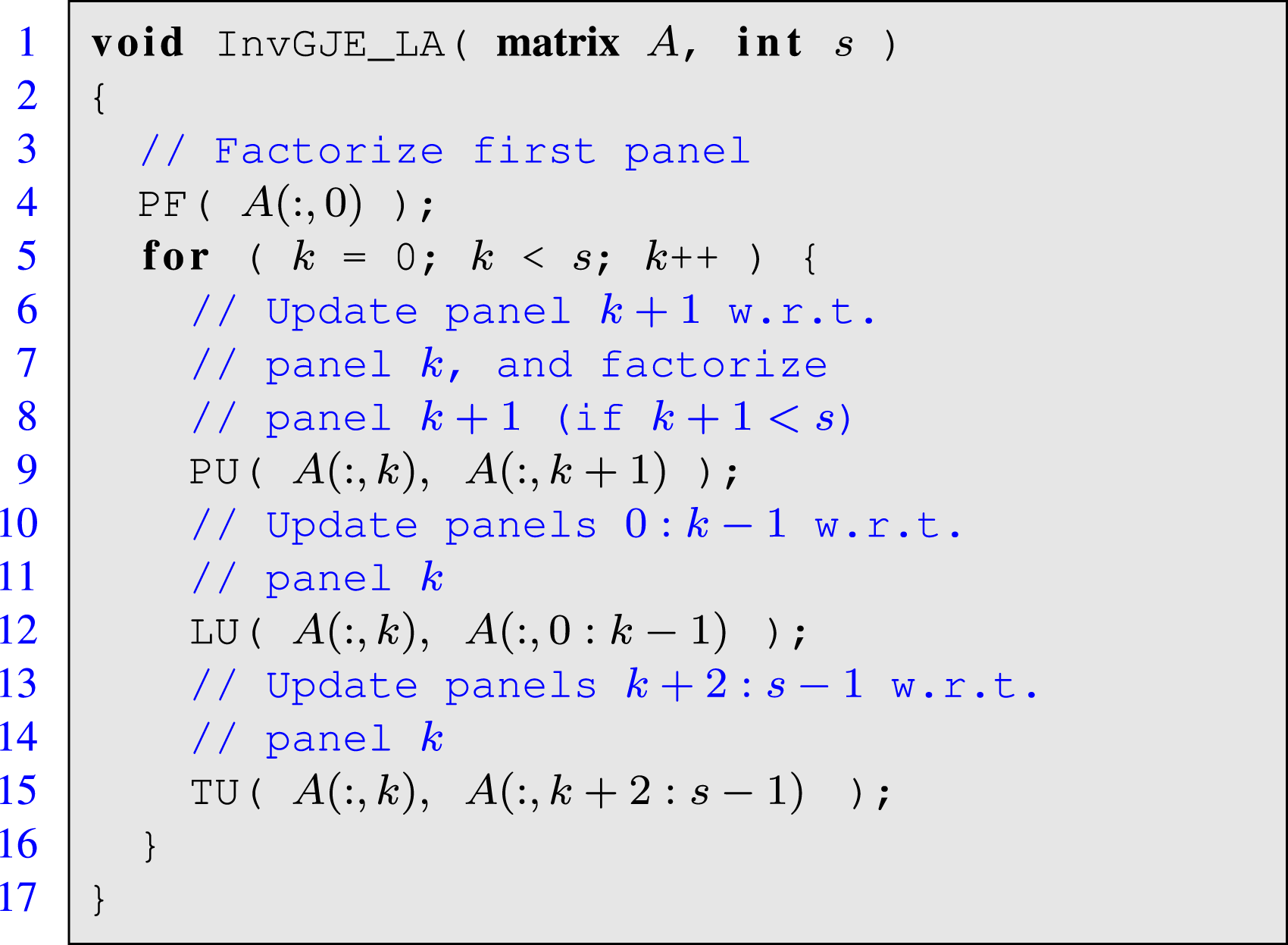
Listing 5: Simplified routine for matrix inversion via GJE with look-ahead.

As for other conventional panel factorizations, such as the LU, QR or Cholesky decompositions, the application of look-ahead (Strazdins, 1998) overcomes the strict dependencies present in the loop body of the matrix inversion procedure via GJE. For this purpose, the trailing submatrix needs to be split into two panels, and the algorithm has to be (manually) re-organized, applying a sort of software pipelining strategy in order to perform the panel factorization of the (k + 1)-th panel in the same iteration as the updates of the leading and trailing submatrices with respect to the factorization k-th panel. These changes allow to overlap the sequential factorization of the “next” panel with the highly parallel update of the “current” leading/trailing submatrices in the same iteration. This is illustrated in the re-organized variant of the algorithm with look-ahead in Listing 5.

The GJE-based algorithm for matrix inversion enhanced with look-ahead features three independent operations per loop iteration: PU, LU and TU. On a multicore processor, the question that arises in this case is how to execute these operations (tasks) in parallel. An straight-forward scheme is to dedicate all threads/cores to computing each operation in a sequential order. That is, all threads compute PU in parallel; upon completion, they next collaborate to compute LU; and, finally, they work on TU, also in parallel. This corresponds to SA + TL. The problem with this scheme is the highly sequential nature of the panel factorization within the panel update, which implies a waste of resources if the block size is even moderately large.

The approach we follow in this work is to divide the collection of threads into three application thread teams, assigning a team consisting only of a few threads to the execution of PU; while dedicating the bulk of the threads, distributed between the remaining two teams, to the execution of LU and TU. Note that, as the iteration progresses, the width (i.e., number of columns) of the submatrix involved in LU increases while that of TU diminishes. In this scenario, the use of a MLB for the execution of the operations underlying LU and TU can allow to shift the threads from one team to the other(s) as soon as they complete the execution of their kernel.

Performance evaluation

Figure 4 compares the following codes for the inversion of an n × n nonsingular matrix:

– MKL. The multi-threaded implementation of this operation in Intel MKL performed via the invocation of routine dgetrf followed by dgetri.

– SINV + MKL/BLIS. Our implementation of the inversion based on GJE, linked with multi-treaded (TL) instances of either Intel MKL or BLIS to execute the kernels invoked from within the LAPACK routine. This corresponds to the SA + TL scheme.

– TINV + LA. A variant of the previous implementation, enhanced with look-ahead. Task parallelism is exploited in this case using the OpenMP runtime and loop-parallelism from within linear algebra TL. This is the baseline for the TA + TL scheme.

– TINV + MLB. Same variant as TINV + LA, but linked with the malleable version of BLIS.

Figure 4.

Performance of the matrix inversion.

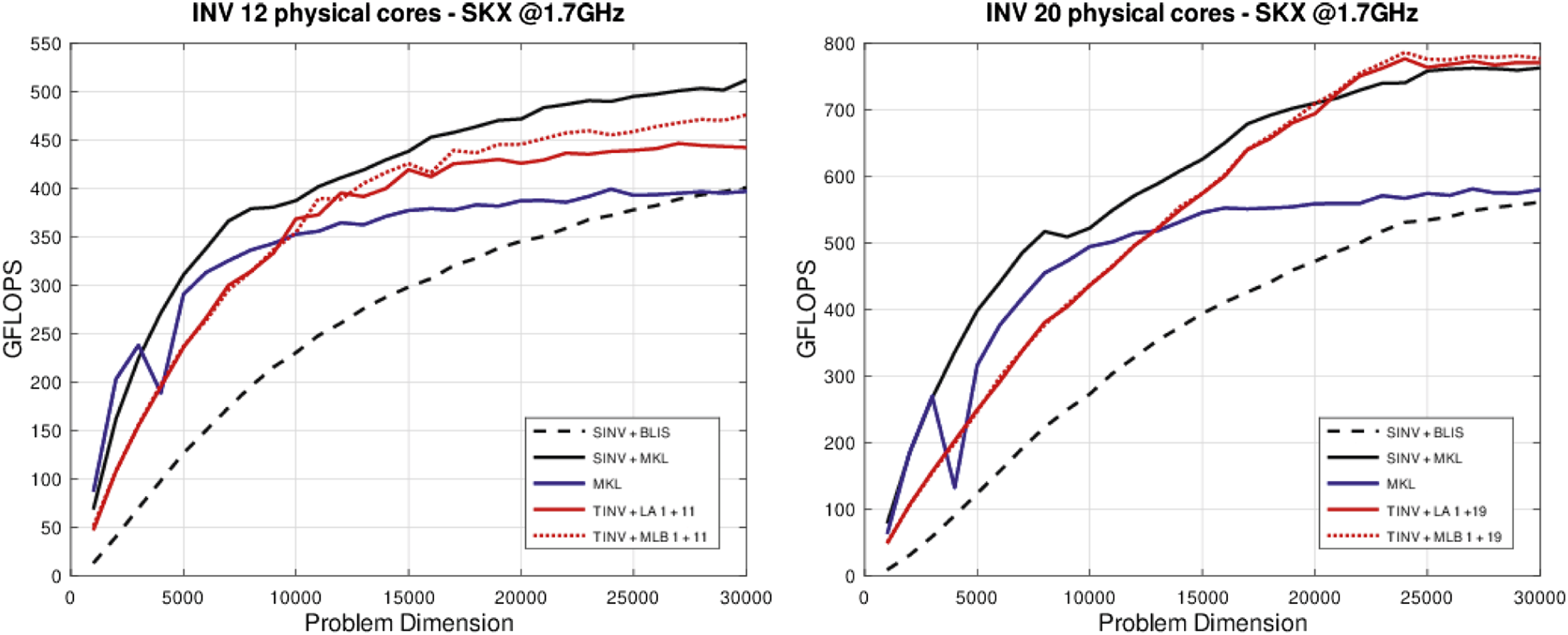
For the last two options we assign a single-thread team to the panel “factorization”; the remaining threads are then split among the two other teams, in charge of the left and right panel updates, depending on the cost of these operations. We also evaluated other options with 2 and 3 threads mapped to the team in charge of the panel, but they showed inferior performance for this operation. Both TINV + LA and TINV + MLB are TA + TL schemes. In all cases (except MKL), the algorithmic block size was manually tuned to optimize performance.

Figure 4 shows that the variant TINV + MLB matches or even improves the performance of TINV + LA both with 12 and 20 cores (by up to 9% and 3%, respectively). However, in some cases, the malleability gains may seem minor in comparison with SINV + MKL. Note that, in order to implement TINV + MLB, some of the Intel BLAS kernels needed to be replaced by their counterparts in BLIS, and the overall performance might suffer from this change. This effect can be clearly observed when contrasting the SINV versions, which show a substantial performance increase when using Intel MKL, due to the performance differences of the underlying basic kernels in MKL and BLIS. Regarding the MKL implementation, in general our GJE-based versions deliver higher performance thanks to a better distribution of the workload between iterations.

Deep learning inference

Inference algorithms

Deep neural networks (DNNs) consist of a large collection of interconnected neuron layers, where each layer performs an operation on its inputs to produce the output activations that are passed to the next layer. In the inference process for convolutional neural networks (CNNs), to a large extent these computations are equivalent to a general matrix-matrix multiplication (GEMM) or a convolution (Higham and Higham, 2018), followed by the elementwise application of a non-linear function. Furthermore, under certain conditions, the convolutions can be efficiently cast in terms of an enlarged GEMM via the im2col transform (Chellapilla et al., 2006).

The inference algorithm is illustrated with a high level of abstraction in Listing 6. There, it consists of an “endless” loop that commences with a blocking call to extract a sample (or collection of samples) from the input buffer I into the activation buffer A₁ (layer 1 or input layer). These data are then serially processed by the sequence of layers that define the model: For l = 2, 3, …, L, layer l receives the input activations A_l−1 and applies the transforms defined by the model in that layer, given by W _l , to produce the outputs for that layer, A _l , which will then become the input activations for the subsequent layer. The final result is passed to the output buffer (layer) O.

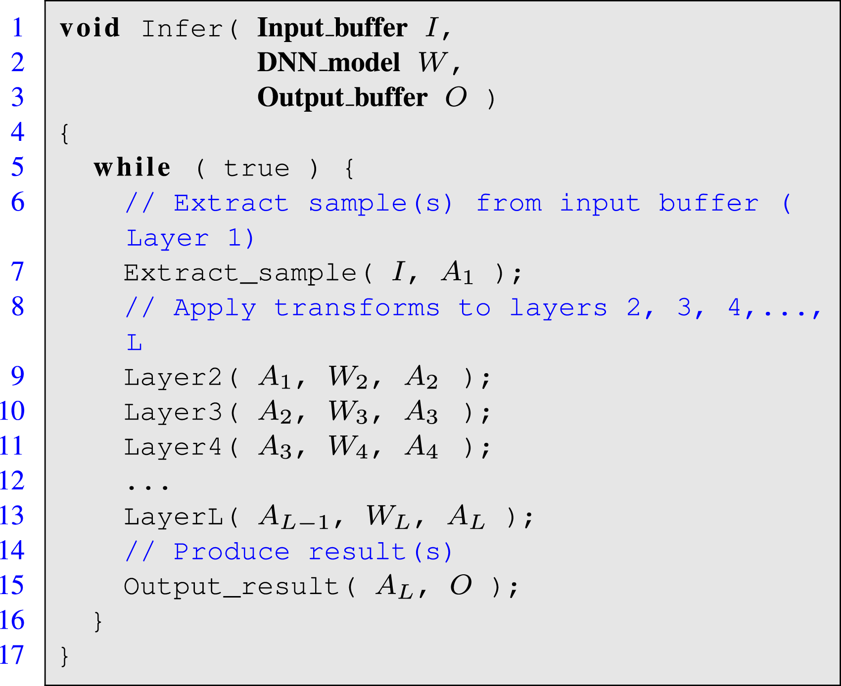
Listing 6: Simplified routine for inference with a DNN consisting of L layers.

The scenario we target in this case study reflects a high-performance inference server operating on the edge, which remains inactive till it receives a sample, e.g., from one among several connected devices, via the input buffer. The server then has to apply a specific DNN model to the batch of samples to produce an output under certain time constraints. While this occurs, new samples can arrive, from the same or other source, being enqueued into the input buffer till the server is ready to process them.

Now, as argued at the beginning of this section, when dealing with CNNs most layers involve a convolution, and this type of kernel dominates the global cost of the inference. For example, a fully-connected (FC) layer with n_l−1 inputs and n _l outputs, that receives a batch of b samples, boils down to a GEMM of dimensions defined by these three parameters: n_l−1, n _l and b. On the other hand, consider a Convolutional layer that comprises a convolution operator consisting of k _n filters (or kernels) of dimension k _h × k _w × c _i each. Assume the layer receives b tensor inputs (or samples) of dimension h _i × w _i × c _i each; and produces b tensor outputs of size h _o × w _o × k _n each. Using the im2col transform, the convolution can then be applied in terms of a GEMM with the dimensions defined by k _n , (h _o · w _o · b) and (k _h · k _w · c _i ). Other types of DNN layers, such as batch normalization, regularization, flatten or pooling present a minor contribution to the arithmetic cost and execution time of a DNN.

The challenges for the inference process on a multicore process arise from the constraints on the response times for many practical applications (e.g., real-time object recognition), the unpredictable arrival time of the batches (and sometimes even the number of samples of each batch), and the unbalanced computational costs of the distinct layers. Under these conditions, an SA + TL scheme prioritizes the execution of the “current” batch but may violate a service level agreement on the response time of pending batches in the input buffer; besides, it may result in a waste of threads during the execution of layers that involve small GEMMs. In addition, a TA + SL scheme may produce a suboptimal execution due to conflicts during the access to shared resources such as the main memory and (certain levels of) cache; also, if the number of batches in the input buffer is small, the degree of task-parallelism is low, and several threads will remain idle. The third option is to follow the TA + TL scheme, possibly enhanced with malleability.

Performance evaluation

The experiments for the deep learning (DL) use case in this section were carried out in a platform equipped with a 48-core ARMv8 processor (Huawei Kunpeng 920). As in the previous cases, the malleability mechanism was integrated into BLIS v0.5.1 (Rodríguez-Sánchez et al., 2020). On this platform, gcc 7.5.0 was used as the compiler and the codes were linked with OpenMP 4.5. All experiments were performed using 24 cores and IEEE 32-bit floating point arithmetic. The operating frequency for all cores was set to 2.6 GHz.

The DNN model that is employed for the following evaluation corresponds to ResNet-50 (He et al., 2016) (but Similar results were obtained for AlexNet as well as variants of VGG models). We analyze two variants of an scenario that emulates, for example, an autonomous car equipped with several cameras that capture and send images to a centralized inference server (in the vehicle). In both cases, the server processes the images (samples) in batches, with each batch comprising the samples received in the last 0.1 s. In the first case, each batch contains the same number of samples: either 1, 2, 4 or 8 in our experiments. In the second case, each batch may now consist of a distinct number of samples: between 1 and 8. These two variants reflect cases where all the cameras capture images at the same rate or at different rates, respectively. (The inter-batch period was selected to emphasize the differences between the distinct parallelization schemes presented next.)

We consider 7 parallelization schemes for the DL case study: the baseline configuration (labelled as SDL–BLIS) leverages all resources (deploying 24 threads and hence using 24 cores) to run inference for a single batch at a time. Alternatively, there are three schemes that divide these resources into two, three or four teams (with either 12, 8 or 6 threads/cores per team, respectively), with these teams in charge of the simultaneous execution of two, three or four concurrent batches (labelled as TDL 12 + 12, TDL 8 + 8+8 and TDL 6 + 6+6 + 6). These multi-team parallelization schemes have their malleable counterparts, linked with a malleable version of BLIS, that asymmetrically divide the threads into 8 + 16 (two teams), 7 + 7 + 10 (three teams) or 5 + 5 + 5 + 9 (three teams). In these malleable solutions, a team is formed by a single OpenMP thread that spawns as many BLIS threads as required. For example, when there are two teams, two OpenMP threads are created at the beginning and each one spawns 11 additional BLIS threads for the calculations. In DL, all the teams execute exactly the same code but load imbalance can still appear because the teams may be executing distinct DNN layers at a certain moment or they have to deal with batches of different size. In this case study, we leverage malleability in order to increase the number of resources assigned to a team that is “currently” executing a costly layer. In ResNet-50, this mostly occurs during the execution of the first layer (due to the dimensions of the convolution being executed in that layer). Thus, the goal is that a team which commences the execution of that layer, borrows threads from the other teams. For example, in the case of three teams (with 7, 7, and 10 threads per team) when one of them reaches the execution of the first layer, it sets the number of threads of the other teams up to 7 and its own number of threads is increased to 10.

We analyze the performance of the previously-described schemes using three key metrics: 1) the total execution time necessary to process a certain number of batches; 2) the execution time per batch; and 3) the waiting time per batch (that is, the time from the moment the batch arrives to the input queue till it is processed). The total execution time highlights the benefits of a concurrent execution of multiple batches. On the one hand, the execution time per batch illustrates the performance hit due to the increase of the number of teams (which results in a decreasing number of threads per team). On the other hand, the waiting time per batch shows the real benefits of the multi-team execution from the point of view of satisfying a given constraint in the time response.

The top two plots in Figure 5 demonstrate that increasing the number of concurrent teams reduces the total execution time for inference with batches of both fixed and variable size. The reason is that the layers of RestNet-50 are not complex enough (from the computational perspective) to fully profit from the 24 cores. As a result, the execution of several inference processes in parallel reduces the total execution time by a factor of 1.85× when using two teams, 2.4× with three teams, and a factor of 2.7× with four teams, for both fixed and variable batch-size scenarios. Malleability contributes a performance gain of up to 5% (two teams), 10% (three teams), and 13% (four teams) in the case of fixed batch size, and up to 4% (two teams), up to 3% (three teams), and up to 4% (four teams) in the case of variable batch size.

Figure 5.

Total execution time, average execution time per batch, and average waiting time per batch (top, middle and bottom, respectively) to perform inference for ResNet-50 with 50 batches of various sizes (left) and three workloads of batches with random sizes (right).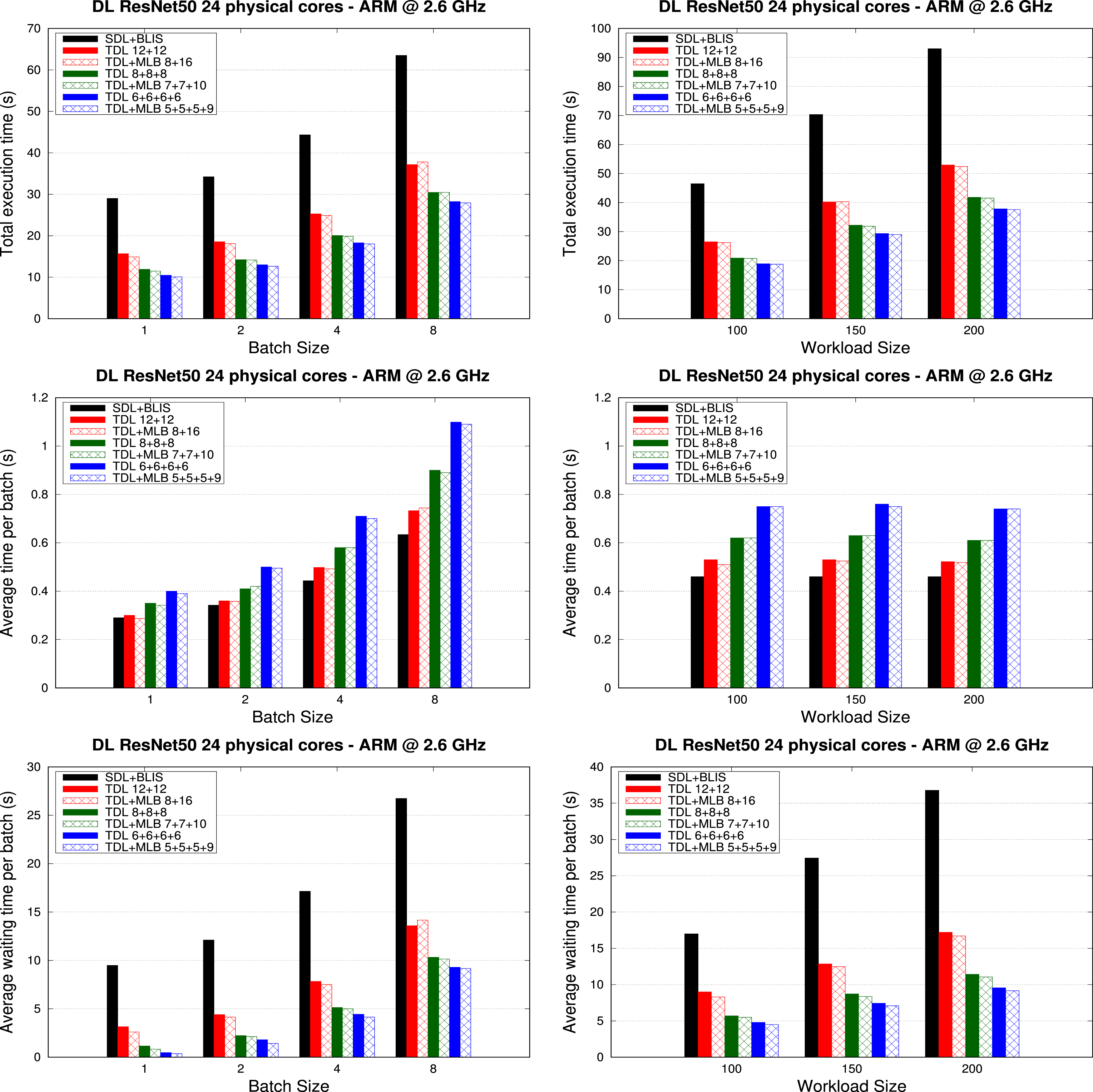

The plots in the middle row of Figure 5 report the average execution time. The results there show that adding more teams (which implies reducing the resources per team), increases the execution time per batch. This growth is not linear with the batch size, because some layers involve memory bound computations, with reduced parallel scalability. Moreover, we observe that dividing the resources between two teams does not increase the execution time per batch. The reason is the low complexity of the individual layers, which does not permit that the two-team scheme benefits from all the computational power of the processor. However, adding the third team results in an increment of the execution time per batch. The effect of the malleability is visible when compared with its corresponding non-malleable counterpart, with a reduction time for the two-team scheme of up to 11% and batch size of 4 and up to 7% with a random batch size. For the three-team scheme, the performance gain is up to 4% in the former scenario and up to 3% with the random batch size. For the four-team scheme, malleability adds a 4% of improvement for fixed batch size and up to 5% for the random scenario. There is also a performance loss for the two-team scheme when the batch size is fixed. This may be due to the negative effect of one team stealing a thread from another team which may be also executing a critical layer. This performance penalty is compensated not only in the total execution time but also in the average waiting time per batch. (That is, the time spent since the batch arrival to the start of its execution.)

Finally, the bottom two plots in Figure 5 illustrate the benefits of increasing the number of concurrent execution teams in the waiting time per batch: Using two, three and four teams diminish the average waiting time by factors up to 3×, 8× and 26× when the batch size is fixed; and up to 2.13×, 3.22×, and 3.8× when the batch size is variable; respectively. As in the previous tests, the malleability delivers an extra performance gain, of up to 12%, 14% and 23% for two, three and four teams, respectively.

Conclusions

In this paper, we have assessed the benefits of integrating malleability into the BLIS framework to avoid the rigidity of current instances of BLAS, for which the number of threads used for the execution of a routine is fixed from the beginning to the end. In practice, this new functionality is exposed to the programmer via a minimal modification of the BLIS expert API. The programmer just needs to identify where the distribution of the computation threads must be modified and the change is seamless.

The performance results demonstrate that the benefits of this approach are widely appealing in scenarios where the parallelism is extracted at both application- and library-level. More specifically, when the workload is not equally balanced at application-level, the malleability allows us to modify, at runtime, the parallelism at the library-level with the purpose of improving the overall core occupation.

Considering future work, we believe that malleability can also offer significant advantages in runtime-based task scheduling or popular task-based programming models such as StarPU (Augonnet et al., 2011) and OmpSs (Duran et al., 2011). There, the scarce task-level parallelism in some parts of the application (Dolz et al., 2015) can be by-passed by means to dynamically increasing the parallelism within the tasks. Hence, a fully malleable underlying library becomes mandatory.