
Abstract
A high-performance implementation of a multiphase lattice Boltzmann method based on the conservative Allen-Cahn model supporting high-density ratios and high Reynolds numbers is presented. Meta-programming techniques are used to generate optimized code for CPUs and GPUs automatically. The coupled model is specified in a high-level symbolic description and optimized through automatic transformations. The memory footprint of the resulting algorithm is reduced through the fusion of compute kernels. A roofline analysis demonstrates the excellent efficiency of the generated code on a single GPU. The resulting single GPU code has been integrated into the multiphysics framework waLBerla to run massively parallel simulations on large domains. Communication hiding and GPUDirect-enabled MPI yield near-perfect scaling behavior. Scaling experiments are conducted on the Piz Daint supercomputer with up to 2048 GPUs, simulating several hundred fully resolved bubbles. Further, validation of the implementation is shown in a physically relevant scenario—a three-dimensional rising air bubble in water.
1. Introduction
The numerical simulation of multiphase flow is a challenging field of computational fluid dynamics (see Prosperetti and Tryggvason, 2007). Although a wide variety of different approaches have been developed, simulating the dynamics of immiscible fluids with high-density ratio and at high Reynolds numbers is still considered complicated (see Huang et al., 2015). Such multiphase flows require models for the interfacial dynamics (see Yan et al., 2011). A full resolution of these phenomena is usually impractical for macroscopic CFD techniques since the interface is only a few nanometers thick as pointed out by Fakhari et al. (2017b).
Therefore, sharp interface techniques model the interface as two-sided boundary conditions on a free surface and can thus achieve a discontinuous transition (see Bogner et al., 2015; Körner et al., 2005; Thürey et al., 2009). The modeling and implementation of these boundary conditions can be complicated as stated by Bogner et al. (2016), especially in a parallel setting. Diffuse-interface models, in contrast, represent the interface in a transition region of a finite thickness that is typically much wider than the true physical interface (see Anderson et al., 1998). Thus, the sharp interface between the fluids is replaced by a smooth transition with thickness
Typically, the simulation domain is discretized with a Cartesian grid for 3D LBM simulations. Due to its explicit time-stepping scheme and its high data locality, the LBM is well suited for extensive parallelization (see Bauer et al., 2020a). For the simulation of multiphase flows, additional force terms are needed that employ non local data points so that the ideal situation may worsen somewhat. Fakhari et al. have shown how to improve the locality for the conservative ACM (see Fakhari et al., 2017b). In order to resolve physically relevant phenomena, a sufficiently high resolution at the interface between the fluid phases is necessary. Thus we may need simulation domains containing billions of grid points and beyond. This creates the need for using high-performance computing (HPC) systems and for a highly parallelized and run-time efficient algorithms. However, highly optimized implementations in low-level languages like Fortran or C often suffer from poor flexibility and poor extensibility so that algorithmic changes and the development of new models may get tedious.
To overcome this problem, we here use a work flow where we generate the compute intensive kernels at compile time with a code generator realized in Python. Thus we obtain the highest possible performance while maintaining maximal flexibility (see Bauer et al., 2019). Furthermore, the symbolic description of the complete ACM allows us to use IPython (see Pérez and Granger, 2007) as an interactive prototyping environment. Thus, changes in the model, like additional terms, different discretization schemes, different versions of the LBM or different LB stencils can be incorporated directly on the level of the defining mathematical equations. These equations can be represented in LaTeX-form. The generated code can then run in parallel with OpenMP parallel on a single CPU or on a single GPU. Once a working prototype has been created in this working mode, the automatically generated code kernels can be integrated into existing HPC software as external C++ files. In this way, we can execute massively parallel simulations. Note that this workflow permits to describe physical models in symbolic form and still run with maximal efficiency on parallel supercomputers. Using code generation, we realize a higher level of abstraction and thus an improved separation of concerns.
The remainder of the article is structured as follows. In Section 2, we will summarize related work to the conservative ACM. In Section 3, we will introduce the governing equations of the conservative ACM. Section 4 presents details of the implementation, by first introducing the code generation toolkit lbmpy by Bauer et al. (2020b) which constitutes the basis of our implementation. Then, we present the phase-field algorithm itself in a straightforward and an improved form, where the improvements essentially lie in the minimization of the memory footprint. This is primarily achieved by changing the structure of the algorithm in order to be able to fuse several compute kernels. The performance of our implementation is discussed in Section 5. We first show a comparison of the straightforward and the improved algorithm. Then the performance of the improved version is analyzed on a single GPU with a roofline approach. After that the scaling behavior on up to
2. Related work
The interface tracking in this work is carried out with the Allen-Cahn equation (ACE) (see Allen et al., 1976). A modification of the ACE to a phase-field model was proposed by Sun and Beckermann (2007). Nevertheless, it is Cahn-Hilliard theory (see Cahn and Hilliard, 1958), which is most often used in phase-field models to perform the interface tracking. A reason for that is the implicit conservation of the phase-field and thus the conservation of mass. As a drawback, it includes fourth-order spatial derivatives, which worsens the locality of the LB framework as pointed out by Geier et al. (2015a). In order to make the ACE accessible for phase-field models, Pao-Hsiung and Yan-Ting (2011) have presented it in conservative form. Furthermore, the conservative ACE contains only second-order derivatives which allows a more efficient implementation.
In the work of Geier et al. (2015a) the conservative ACE was first solved using a single relaxation time (SRT) algorithm. Additionally, they proposed an improvement of the algorithm by solving the collision step in the central moment space and adapting the equilibrium formulation which makes it possible to directly calculate the gradient of the phase-field locally via the moments. This promising approach, however, leads to a loss of accuracy (see Fakhari et al., 2019). On the other hand Fakhari et al. (2017b) used an SRT formulation to solve the conservative ACE with isotropic finite-differences (see Kumar, 2004) to compute the curvature of the phase-field. This approach was later extended by Mitchell et al. (2018a) for the three-dimensional case. A disadvantage of this approach is, that it becomes complicated to apply single array streaming patterns (see Wittmann et al., 2016) like the AA-pattern or the Esoteric Twist to the LBM as stated by Geier et al. (2015a). This is due to a newly introduced non-locality in the update process, originating in the finite difference calculation (see Geier et al., 2015a). In this publication, the phase-field LBE is presented with a multiple relaxation time (MRT) formulation which was first published by Ren et al. (2016). This formulation was also used in recent studies by Dinesh Kumar et al. (2019).
3. Model description
3.1. LB model for interface tracking
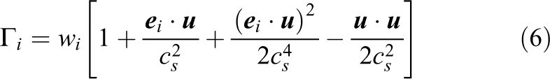
As described by Fakhari et al. (2017b), the phase-field
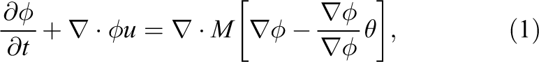
where

is related to the phase-field relaxation time
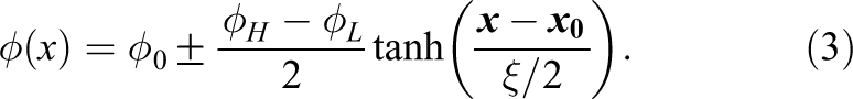
In the equilibrium state the profile of the phase-field
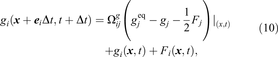
The LB model for equation (1) to update the phase-field distribution function hi can be written as (see Geier et al., 2015a)
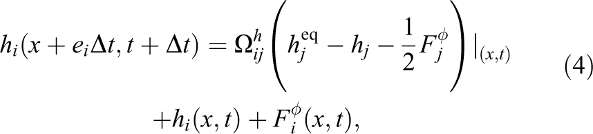
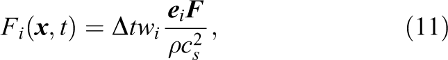
in which the forcing term is given by (see Fakhari et al., 2017b)
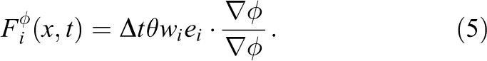
In equation (4)
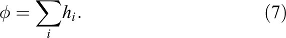
is the dimensionless distribution function. By taking the zeroth moment of the phase-field distribution functions the phase-field
The density

where
3.2. LB model for hydrodynamics
In a macroscopic form the continuity and the incompressible Navier-Stokes equations describe the evolution of a flow field and can be written as
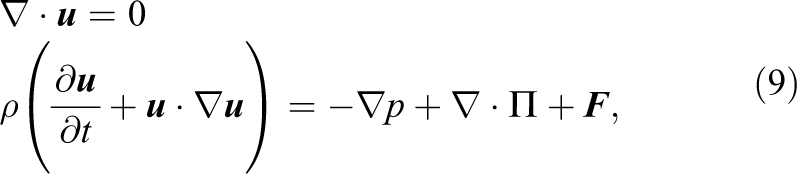
where
where the hydrodynamic forcing is given by
and gi is the velocity-based distribution function for incompressible fluids. The equilibrium distribution function is

where

The pressure force can be obtained as

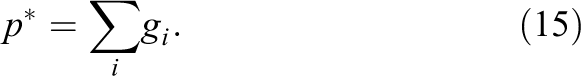
where the normalized pressure is calculated as the zeroth moment of the hydrodynamic distribution function
The surface tension force

is the product of the chemical potential

and the gradient of the phase-field. The coefficients
where the viscosity

There are a few different ways to interpolate the hydrodynamic relaxation time as it is shown in the work of Fakhari et al. (2017b). Overall, they have demonstrated to get the most stable results with a linear interpolation. Therefore, we will use it in this work

We relax the second-order moments with the hydrodynamic relaxation rate
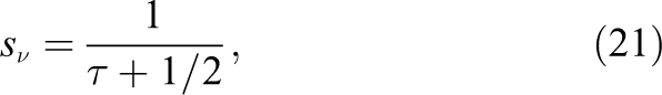
when solving equation (10) to ensure the correct viscosity of the fluid. All other moments are relaxed by one. The velocity u is obtained via the first moments of the hydrodynamic distribution function and gets shifted by the external forces
In order to approximate the gradient in equations (5), (14), (16) and (18) a second-order isotropic stencil can be applied (see Kumar, 2004; Ramadugu et al., 2013)
The Laplacian in equation (17) can be approximated with
4. Software design for a flexible implementation
4.1. Code generation
Our implementation of the conservative ACM is based on the open-source LBM code generation framework lbmpy 1 (see Bauer et al., 2020b). Using this meta-programming approach, we address the often encountered trade-off between code flexibility, readability, and maintainability on the one hand, and platform-specific performance engineering on the other hand. Especially when targeting modern heterogeneous HPC architectures, a highly optimized compute kernel, may require that loops are unrolled, common subexpressions extracted, and possibly hardware-specific intrinsics are used. In state-of-the art optimized software (see Hager and Wellein, 2010), these transformations are essential, and must be performed manually for each target architecture. Clearly, the resulting codes are time-consuming to develop, error prone, hard to read, difficult to maintain and often very hard to adapt and extend. Flexibility and maintainability have been sacrificed, since such complex programming techniques are essential to get the full performance available on the system.
Here, in contrast, we employ the LBM code generation framework lbmpy. Thanks to the automated code transformations, the LB scheme can be specified in a high-level symbolic representation. The hardware- and problem-specific transformations are applied automatically so that starting from an abstract representation, highly efficient C-code for CPUs or CUDA/OpenCL code for GPUs can be generated with little effort.
Our new tool lbmpy is realized as a Python package that in turn is built by using the stencil code generation and transformation framework pystencils 2 (see Bauer et al., 2019). The flexibility of lbmpy results from the fully symbolic representation of collision operators and compute kernels, utilizing the computer algebra system SymPy (see Meurer et al., 2017). The package offers an interactive environment for method prototyping and development on a single workstation, similar to what FEniCS (see Alnæs et al., 2015) is in the context of finite element methods. Generated kernels can then be easily integrated into the HPC framework waLBerla, which is designed to run massively parallel simulations for a wide range of scientific applications (see Bauer et al., 2020a). In this workflow, lbmpy is employed for generating optimized compute and communication kernels, whereas waLBerla provides the software structure to use these kernels in large scale scenarios on supercomputers. lbmpy can generate kernels for moment-based LB schemes, namely single-relaxation-time (SRT), two-relaxation-times (TRT), and multiple-relaxation-time (MRT) methods. Additionally, modern cumulant and entropically stabilized collision operators are supported (see Geier et al., 2015b; Karlin et al., 1998).
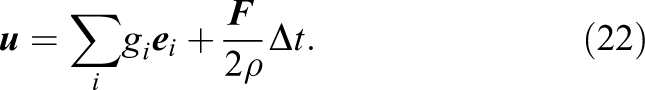
When implementing the coupled multiphase scheme as described in Section 3 with lbmpy, we can reuse several major building blocks that are already part of lbmpy (see Figure 1). First we can choose between different single-phase collision operators to use for the Allen-Cahn and the hydrodynamic LBM. We can easily switch between different lattices, allowing us to quickly explore the accuracy-performance trade-off between stencils with more or less neighbors. A native 2D implementation is also quickly available by selecting the D2Q9 lattice model.
Flexibility of the conservative ACM with the lbmpy code generation framework. The boxes on the right show the two LB steps. On the left options are shown which can be applied to the two LB steps by lbmpy. The connecting lines show a possible configuration which will be used for the benchmark in this section.
Then, the selected collision operators of lbmpy can be adapted to the specific requirements of the scheme. In our case, we have to add the forcing terms equations (5) and (13). This is done on the symbolic level, such that no additional arrays for storing these terms have to be introduced, as would typically be the case when extending an existing LB method implemented in C/C++. Also no additional iteration passes are needed to compute the force terms. The additional forces computed directly and are within the loops that update the LB distributions, thus significantly saving memory and operational overhead. Furthermore, optimization passes, like common subexpression elimination, SIMD vectorization via intrinsics, or CUDA index mapping are done automatically by transformations further down the pipeline, the new force terms are fully included in the optimization. Note how this leads to a clean separation of concerns between model development and optimization with obvious benefits for code maintainability and flexibility without sacrificing the possibility to achieve best possible performance.
On the modeling level, this code generation approach and our tools allow the application developer to express the methods using a concise mathematical notation. LB collision operators are formulated in so-called collision space spanned by moments or cumulants (see Coreixas et al., 2019). For each moment/cumulant a relaxation rate and its respective equilibrium value is chosen. For a detailed description of this formalism and its realization in Python see Bauer et al. (2020b).
Similarly, our system supports the mathematical formulation of differential operators that can be discretized automatically with various numerical approximations of derivatives. This functionality is employed to express the forcing terms. The Python formulation directly mimics the mathematical definition as shown in equations (23) and (24), i.e. it provides a gradient and Laplacian operator. The user then can select between different finite difference discretizations, selecting stencil neighborhood, approximation order, and isotropy requirements.
Starting from the symbolic representations, we create the compute kernels for our application. Knowing the details of the model, in particular the stencil types, at compile time allows the system to simplify expressions, and run common subexpression elimination to reduce the number of floating point operations (FLOPs) drastically.
An overview of the complete workflow including the combination of lbmpy and waLBerla for MPI parallel execution is illustrated in Figure 2. As described above the creation of the phase-field model is accomplished directly with lbmpy, which forms a convenient prototyping environment since all equations can be stated as symbolic representations. lbmpy does not only produce the compute kernels, but can generate also the pack and unpack information as it is needed for the MPI communication routines. This is again completely automatic, since the symbolic representations expose all field accesses and thus the data that must be kept in the ghost layers. A ghost layer is a single layer of cells around each subdomain used for the communication between neighboring subdomains. Furthermore, also the routines are generated, to implement the boundary conditions.
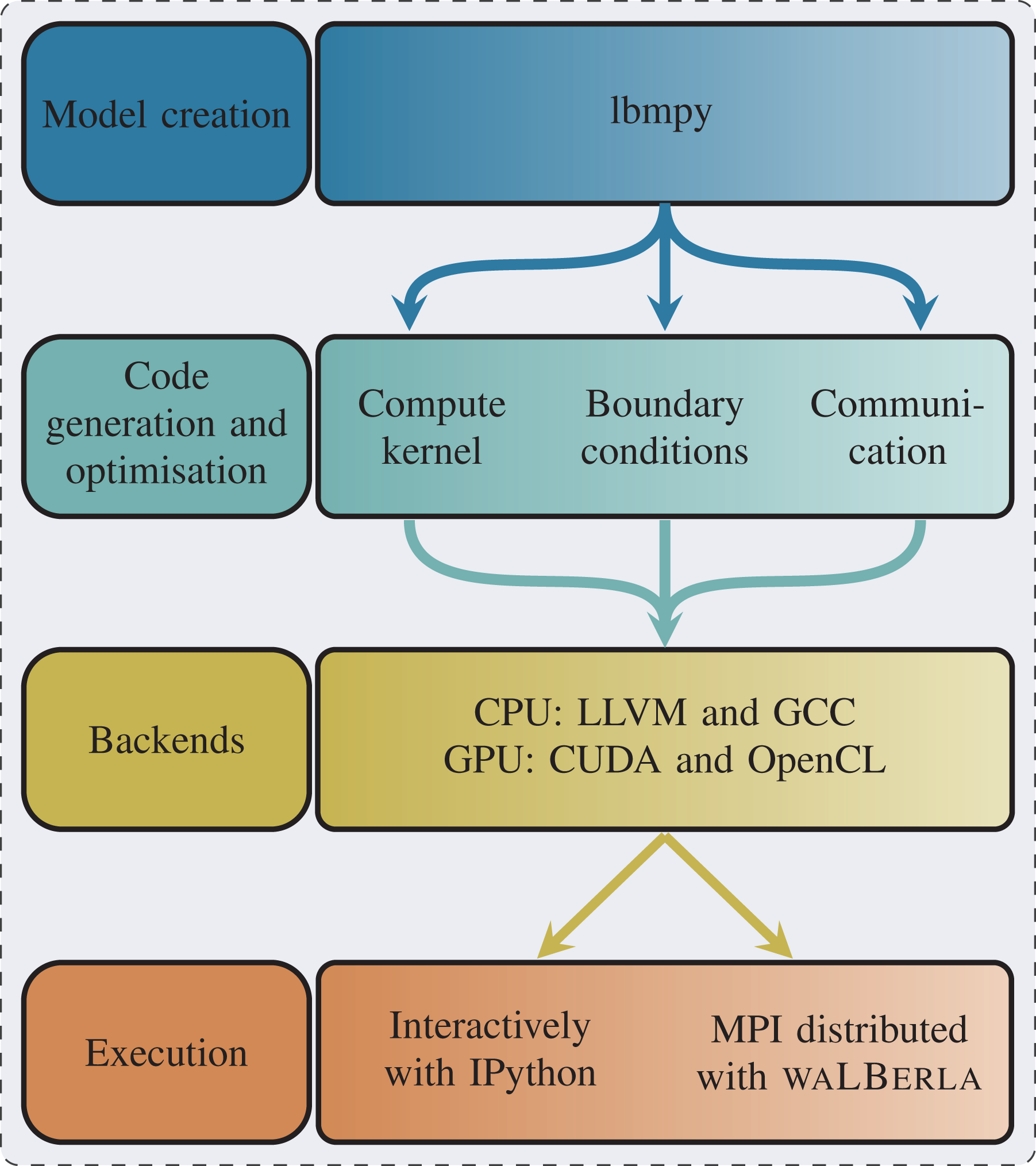
Complete workflow of combining lbmpy and waLBerla for MPI parallel execution. Furthermore, lbmpy can be used as a stand-alone package for prototyping.
The complete generation process can be configured to produce C-Code or code for GPUs with CUDA and alternatively OpenCL. These kernels can be directly called as python functions to be run in an interactive environment or combined with the HPC framework waLBerla .
To demonstrate the usage of lbmpy we show how the update rule for the hydrodynamic distribution functions gi is realized. Following Mitchell et al. (2018b) equation (10), should be formulated as
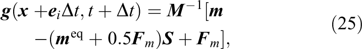
where
4.2. Algorithm
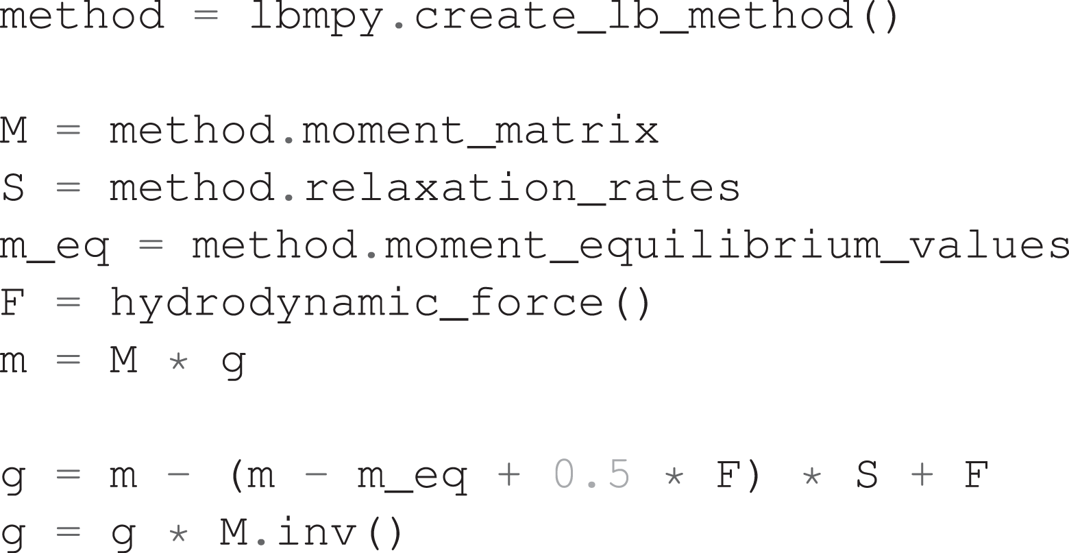
To discuss how the model of Section 3 can be realized, we will first present a straightforward implementation. The corresponding algorithm is displayed in Algorithm 1 and will be discussed briefly in the following. We start the time loop with time step size
Straightforward algorithm for the conservative ACM.
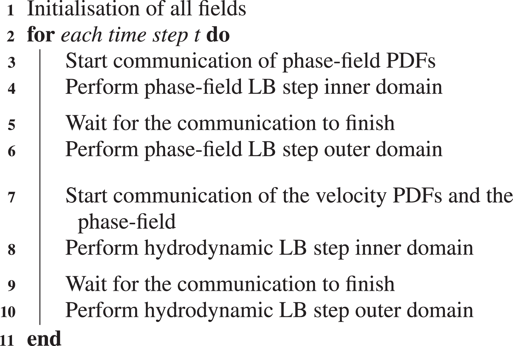
Based on this straightforward algorithm, we will now outline substantial improvements that can be made. To lower the memory footprint of the phase-field model, we combine the collision and the streaming of the phase-field distribution functions and the update of the phase-field into one phase-field LB step. Accordingly, the collision and the streaming of the velocity PDFs and the update of the velocity field get combined to one hydrodynamic LB step. In this manner, the phase-field and velocity PDFs, as well as the phase-field and velocity field, get updated in only two instead of six compute kernels. A detailed overview of the proposed algorithm for the conservative ACM is presented in Algorithm 2. In our proposed algorithm, we subdivide each LB step into iterations over an outer and an inner domain, similarly to Feichtinger et al. (2015) but with variable cell width. This is pointed out in Figure 3. For illustration purposes, the figure illustrates only the two-dimensional case. The three-dimensional case is completely analogous. As shown, the frame width controls the iteration space of the outer and inner domain. This can be done for all directions independently. In the case illustrated, we have a frame width of four cells in x-direction and two grid cells in y-direction.
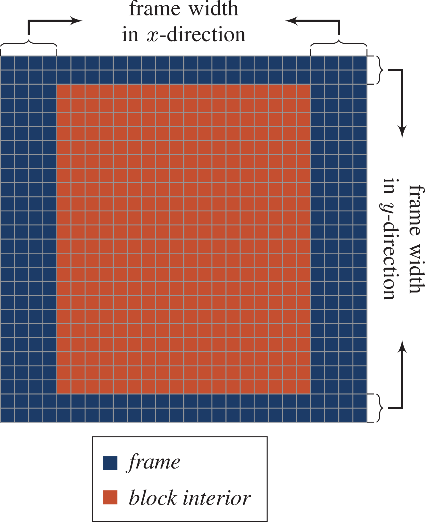
Subdivision of the domain for communication hiding.
After the initialization of all fields, we start the time loop with time step size
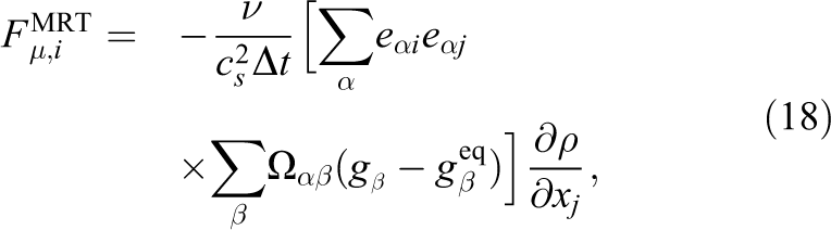
When the LB step for interface tracking is carried out, we start the communication of the velocity-based distribution function together with the phase-field. Note that these communication requirements can now be combined so that only one MPI-message must be sent. Simultaneously, the inner part of the domain gets updated with the hydrodynamic LB step in a collide-stream-push manner. According to equation (18), we need to form the non-equilibrium for the viscous force, which makes a collide-stream-push scheme more convenient to use. To lower the memory pressure, we update the velocity field with equation (22) in the same kernel accordingly. To finish a single time step, we wait for the communication and update the outer part of the domain. Consequently, in Algorithm 2, a one-step two-grid algorithm is applied for both LB steps. In the literature, improvements to the algorithms have been proposed, which do not rely on calculating finite differences Geier et al. (2015a). This allows the use of all optimization techniques, which are available for the LBM, like using a single grid algorithm, e.g. the AA-Pattern or the EsoTwist Wittmann et al. (2016). However, it comes with a loss of accuracy and makes the algorithm less stable. Therefore, we do not use the proposed technique in this work and relay on using two population sets instead.
Improved algorithm for the conservative ACM.
5. Benchmark results
In the following, we compare Algorithm 1 and Algorithm 2. For the straightforward algorithm, we need to load each PDF field three times during a single time step. In the improved algorithm, it is only necessary to load each field once. As we will discuss in Section 5.1 in more detail, the performance limiting factor of the model is the memory bandwidth. Therefore, we expect an increase in the performance of our improved algorithm approximately by a factor of three. To measure the performance of both algorithms, we initialize a squared domain of
In the following sections we first investigate the performance of Algorithm 2 for a single GPU. Afterward, we analyze the scaling behavior on an increasing number of GPUs in a weak scaling benchmark. For all investigations, we use a D3Q15 SRT LB scheme for the interface tracking and a D3Q27 MRT LB scheme for the velocity distribution function similarly to Mitchell et al. (2018a).
5.1. Single GPU
For the performance analysis on a single GPU, we focus on the NVIDIA Tesla V100 due to its wide distribution and its usage in the top supercomputers Summit
3
and Sierra.
4
Further, we discuss the performance on a NVIDIA Tesla P100 because it is used in the Piz Daint
5
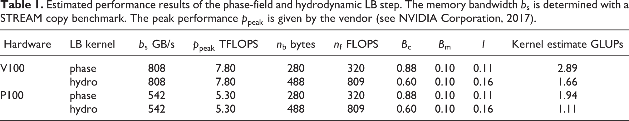
supercomputer, where we ran a weak scaling benchmark which is shown in Section 5.2. In this section, the two LB steps are analyzed independently. In order to determine whether the LB steps are memory- or compute-bound, the balance model is used, which is based on the code balance
and the machine balance
The machine balance describes the ratio of the machine bandwidth
If the “light speed” balance l is less than one a code is memory limited. To be able to calculate l, values for
As specified by the vendor, the V100 has a nominal bandwidth of
The peak performances for the accelerator hardware is taken from the white paper by NVIDIA (see NVIDIA Corporation, 2017). For the V100 a double-precision peak performance of
To determine
For the hydrodynamic LB step, we have a D3Q27 stencil resulting in
In order to get the number of operations, which are executed in one iteration per cell,
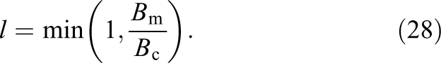
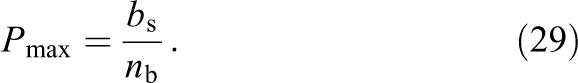
Combining the obtained values in Table 1, we can see that both LB steps are highly memory bound. Therefore, the maximal performance is given by
Estimated performance results of the phase-field and hydrodynamic LB step. The memory bandwidth
Additionally, we profiled the two LB steps with the NVIDIA profiler nvprof 6 for both GPU architectures. The results for the limiting factors are illustrated in Figure 4. These measurements confirm the theoretical performance model very well, and show that the memory bandwidth is almost fully utilized for both GPUs.
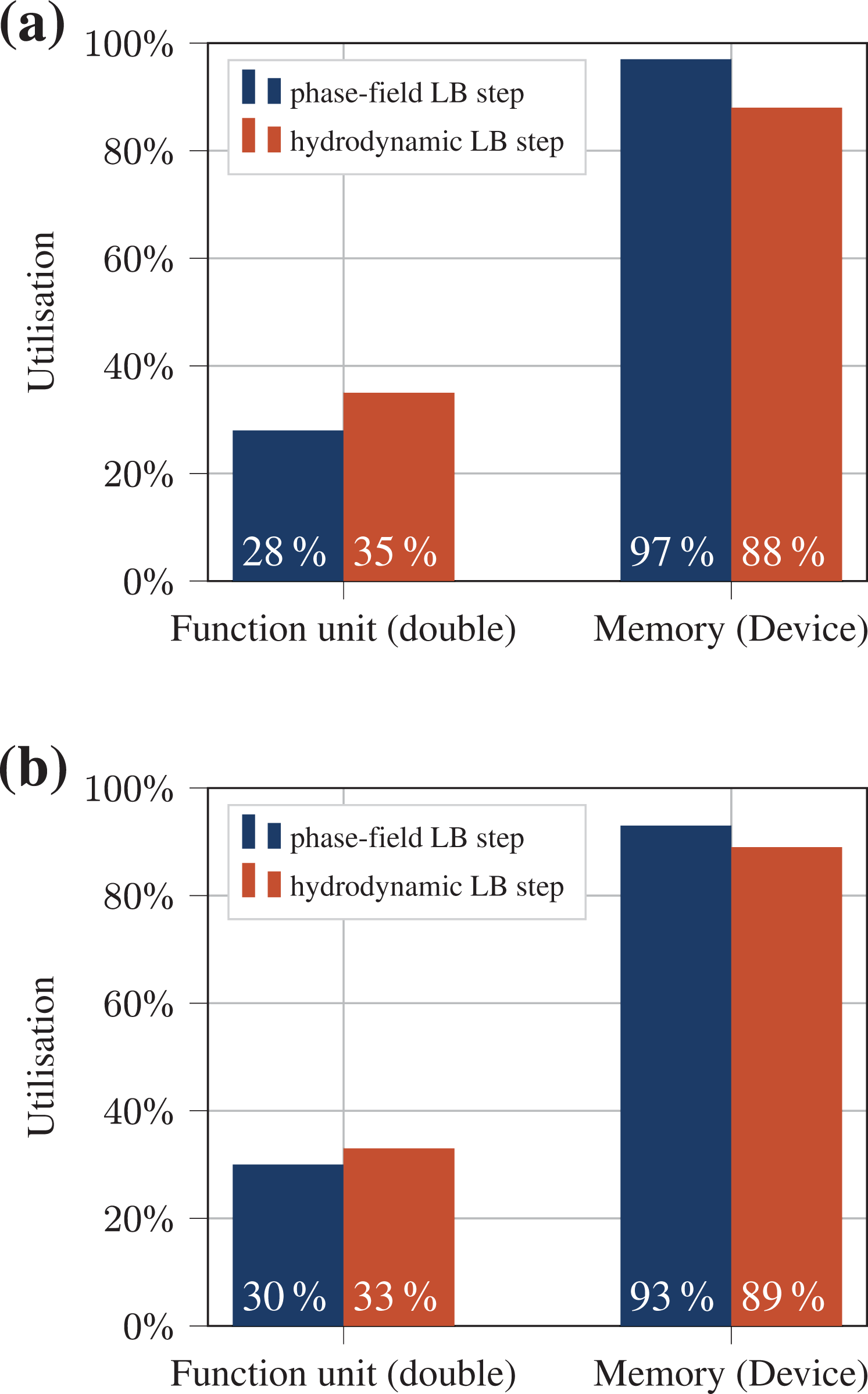
Compute units utilization and memory transfer measured with nvprof (https://docs.nvidia.com/cuda/profiler-users-guide/index.html). The memory transfer is based on the STREAM copy bandwidth of the hardware. The measurements are conducted for the phase-field and the hydrodynamic LB step separately on a Tesla V100 (a) and a Tesla P100 (b).
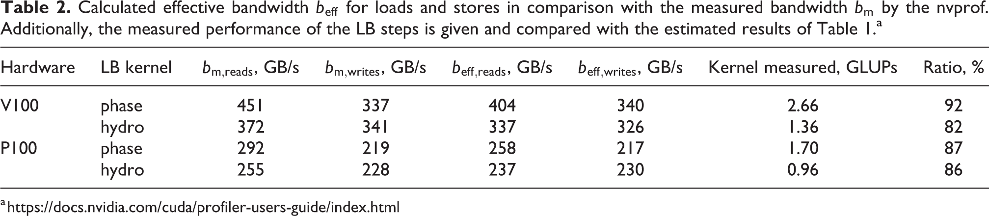
Consequently, the next step is to determine if the memory bandwidth is also reasonable. This means no unnecessary values should be transferred if they are not needed for the calculation. By running the phase-field LB step independently, we measure a performance of about
Calculated effective bandwidth
With the usage of code generation, we can easily change the discrete velocities used for the LB steps of the implementation. This makes it possible for us to evaluate the performance for different two- and three-dimensional stencils. As shown in Figure 5 we employed a D3Q27, D3Q19, D3Q15, and a D2Q9 stencil for both the phase-field and the hydrodynamic LB step. We show that we are able to reach about 86% of the theoretical peak performance for different three-dimensional stencils. This number increases to about 94% on a Tesla V100 and on a Tesla P100 in the two-dimensional case because the assumption that every value of the phase-field
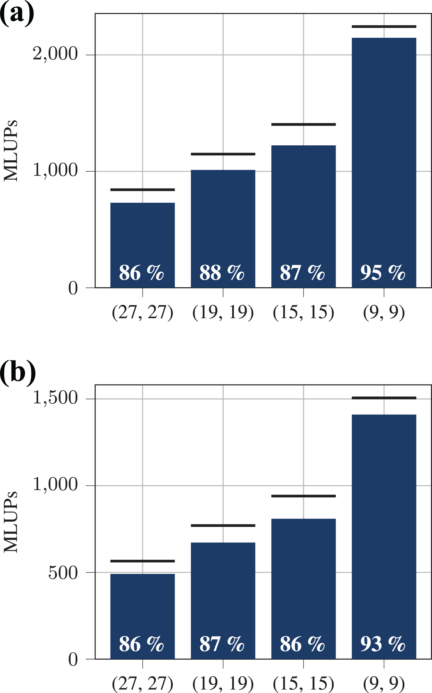
Performance measurement for different LB stencils (D3Q27, D3Q19, D3Q15 and D2Q9) for the phase-field and the hydrodynamic LB step compared to the theoretical peak performances which are illustrated as black lines respectively. The white number in each bar shows the ratio between theoretical peak performance and measured performance. (a) Performance on a Tesla V100. (b) Performance on a Tesla P100.
Due to our implementation’s memory boundness, we expect at most a performance increase by a factor of two when using single precision. However, a detailed analysis of single-precision computation is beyond this work.
5.2. Weak scaling benchmark
The idea of communication hiding for LBM simulations was already studied in Feichtinger et al. (2015). As in Feichtinger et al. (2015) we partition each subdomain (block) into an outer part, to obtain a frame for each block, and an inner part, the block interior. In comparison to that, it is possible in our work, to choose the width of the block frame freely. We can then execute the LBM kernels first on the frame, then send it asynchronously as ghost values to the neighboring blocks. While the communication takes place, the LBM kernels can be executed on the inner domains. Due to our flexible implementation, we ran benchmarks for different frame widths on an increasing number of GPUs in order to find an optimal choice of the frame width. This weak scaling performance benchmark was carried out on the Piz Daint supercomputer on up to
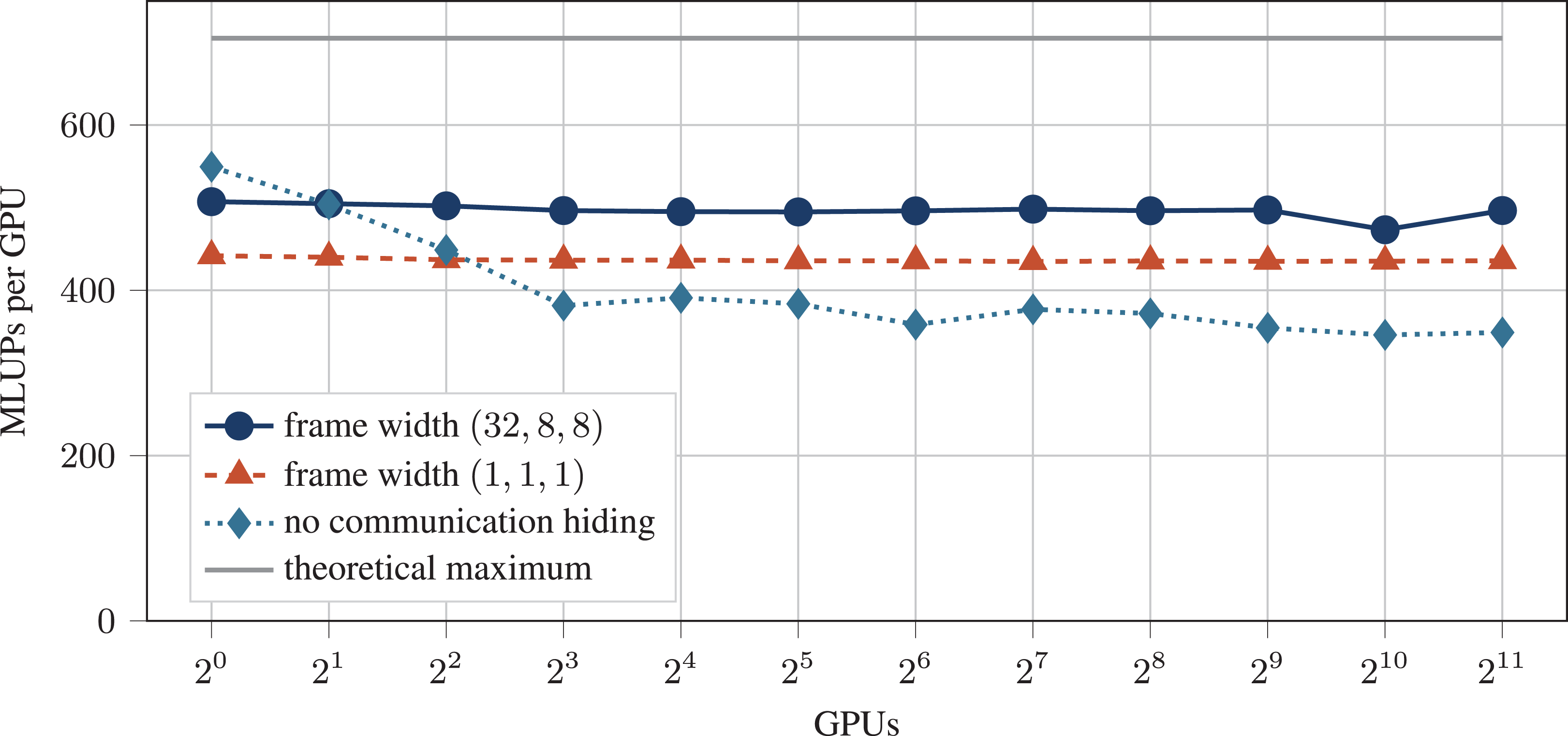
Weak scaling performance benchmark on the Piz Daint supercomputer. The gray line shows the theoretical peak performance. With a thicker frame width (dark blue) we reach a parallel efficiency of almost 98% and also 70% of the theoretical peak performance. Furthermore, it can be seen, that a thin frame (red) shows worse performance and no separation of the domain (light blue) shows worse parallel efficiency.
Both, a frame width of
6. Numerical validation
6.1. Single rising bubble
The motion of a single gas bubble rising in liquid has been studied for many centuries by various authors and is still a problem of great interest today (see Bhaga and Weber, 1981; Clift et al., 1978; Fakhari et al., 2017a; Grace, 1973; Lote et al., 2018; Mitchell et al., 2019; Tomiyama et al., 1998). This is due to its vast importance in many industrial applications and natural phenomena like the aerosol transfer from the sea, oxygen dissolution in lakes due to rain, bubble column reactors and the flow of foams and suspension, to name just a few. Because of the three-dimensional nature and nonlinear effects of the problem, the numerical simulation still remains a challenging task (see Tripathi et al., 2015). The evolution of the gas bubble in stationary fluids depends on a large variety of different parameters. These are the surface tension, the density difference between the fluids, the viscosity of the bulk media and the external pressure gradient or gravitational field through which buoyancy effects are observed in the gas phase. The parameters are developed into dimensionless groups in order to acquire comprehensive theories describing the problem (see Mitchell et al., 2019).
In this study we set up a computational domain of

where gy is the magnitude of the gravitational acceleration, which is applied in the vertical direction
where D is the initial diameter of the bubble. The Eötvös number
which is also called the Bond number describes the influence of gravitational forces compared to surface tension forces. Further, we use the density ratio
Thus, the dimensionless time can be calculated as
Terminal shape of a single rising bubble with
Additionally, we calculate the drag coefficients with the terminal velocity of the bubbles
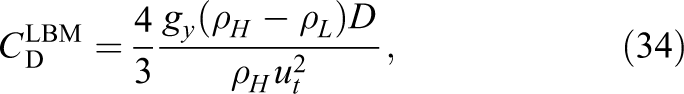
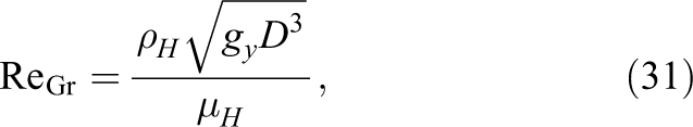
and compare it to the experiments carried out by Bhaga and Weber (1981). Based on their observations they set up the following empirical equation to calculate the drag coefficient of a rising bubble described by the gravity Reynolds number
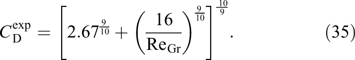
As it can be seen in Figure 8 our results are in good agreement with the experimental investigations.
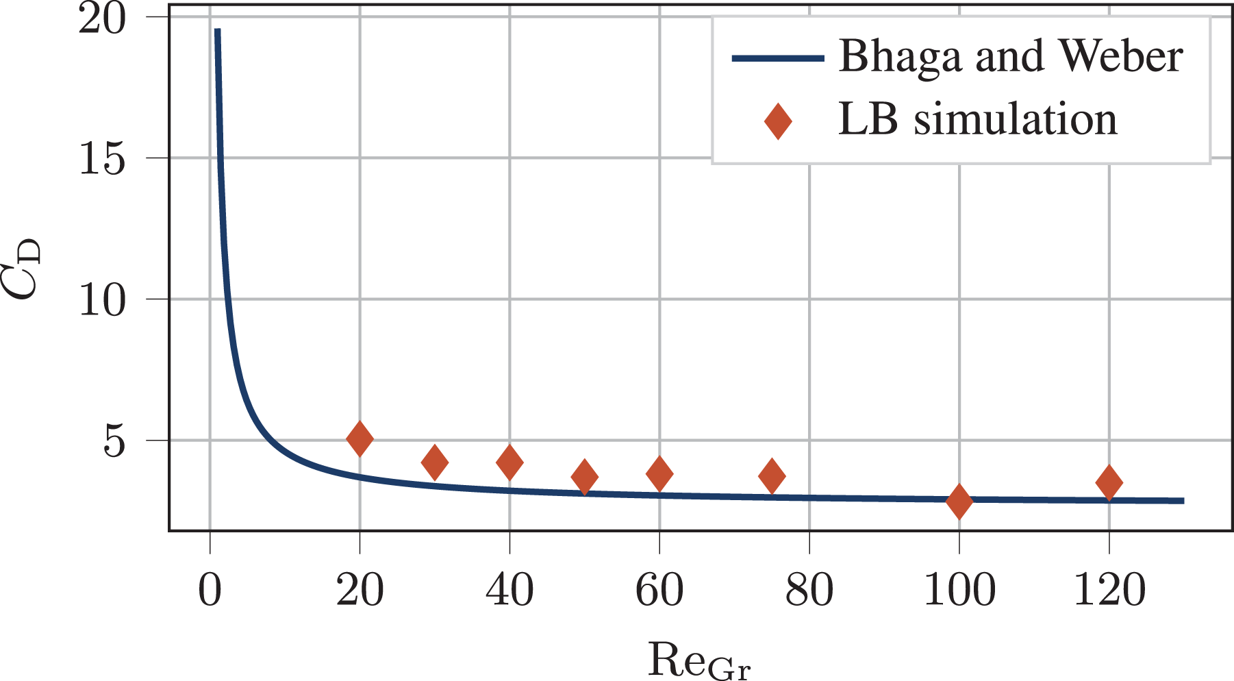
Drag coefficient plotted against the Reynolds number of a single rising bubble. The dots show the results of the LB simulation with a constant Eötvös number of
6.2. Bubble field
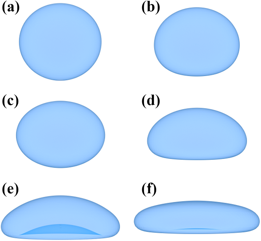
For demonstrating the robustness as well as our possibilities through the efficient and scalable implementation, we show a large scale bubble rise scenario with several hundred bubbles. The simulation is carried out on a
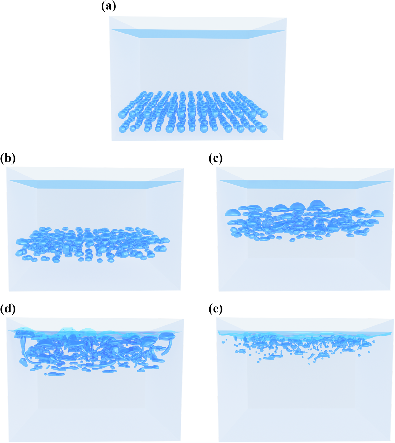
Large scale bubble rise scenario simulated on the Piz Daint supercomputer with several hundred air bubbles. (a) Initialization. (b) Time step 125 000. (c) Time step 250 000. (e) Time step 375 000. (f) Time step 500 000.
7. Conclusion
In this work we have shown an implementation of the conservative ACM based on meta-programming. With this technique we can generate highly efficient C, OpenCL and CUDA kernels which can be integrated in other frameworks for simulating large scale scenarios. For this work we have used the waLBerla framework to integrate our code. We have measured the efficiency our implementation on single GPUs. Excellent performance results compared to the roofline model could be shown for a Tesla V100 and a Tesla P100 where we could achieve about 85% of the theoretical peak performance for both architectures. Additionally, we have shown that our code not only performs very well for one configuration but keeps its excellent efficiency even for different stencils and different methods to solve the LBEs. It is even possible to directly generate 2D cases for testing which also show very good performance results. Through separating our iteration region in an inner and an outer part we could enable communication hiding, relevant for multi-GPU simulations with MPI. With this technique we are able to run large scale simulations with almost perfect scalability. To show this we have run a weak scaling benchmark on the Piz Daint supercomputer on
In the last part of this paper, future work is identified. The interface between two fluids is resolved with several cells in the phase-field model. Thus it is crucial to use a very high resolution. This makes adaptive mesh refinement (AMR) a fundamental approach that should resolve the interface with higher resolution than the bulk fluid (see Fakhari et al., 2017a). Successful usage of AMR with the waLBerla framework in extreme-scale scenarios has been shown in several publications (see Bauer et al., 2020a; Schornbaum and Rüde, 2016, 2018). However, an adaption to GPUs will be future work. With the usage of AMR additional problems will occur, which needs to be tackled. One of those is the strong scaling capability of our implementation. While for weak scaling benchmarks, a single block in our block-structured domain can use the full GPU memory, this is not true anymore if AMR is applied, and thus, smaller refined blocks will be used in parts of the domain. Therefore, it will be important that a single GPU kernel can apply the computation simultaneously to several blocks allocated on the GPU. Otherwise, a GPU compute kernel’s performance will get deteriorate once the block is too small to keep all threads busy. This problem is critical when applying communication hiding strategies done in this work since this divides the individual blocks even further.
While more advanced LB collision operators like the cumulant LBM are available in the lbmpy framework, this has not yet been employed in the phase-field algorithm. As described by Geier et al. (2021), a careful numeric design becomes crucial when using the LBM, especially with more sophisticated collision operators. The annotated symbolic derivation of the algorithm can be made aware of roundoff and stability concerns. In fact, even an automated roundoff error analysis can be developed. This is, however, left to future work.
Footnotes
Acknowledgments
We appreciate the support by Travis Mitchell for this project. Furthermore, we thank Christoph Schwarzmeier and Christoph Rettinger for fruitful discussions on the topic.
Declaration of conflicting interests
The author(s) declared no potential conflicts of interest with respect to the research, authorship, and/or publication of this article.
Funding
The author(s) disclosed receipt of the following financial support for the research, authorship, and/or publication of this article: We are grateful to the Swiss National Supercomputing Centre (CSCS) for providing computational resources and access to the Piz Daint supercomputer. Further, the authors would like to thank the Bavarian Competence Network for Technical and Scientific High Performance Computing (KONWIHR), the Deutsche Forschungsgemeinschaft (DFG, German Research Foundation) for supporting project 408059952 and the Bundesministerium für Bildung und Forschung (BMBF, Federal Ministry of Education and Research) for supporting project 01IH15003A (SKAMPY).
Supporting information
Notes
Author biographies
Markus Holzer is a research assistant at the Chair for System Simulation at the University Erlangen-Nürnberg. He holds a MSc degree in Computational Engineering and is one of the core developers of the waLBerla HPC framework and leading developer of the code generation frameworks pystencils and lbmpy. His research interests are code generation for lattice Boltzmann methods and large scale fluid simulations on heterogeneous and massively parallel hardware.
Martin Bauer is a research assistant at the Chair for System Simulation at the University Erlangen-Nürnberg. He holds a MSc(hons) degree in Computational Engineering and is one of the core developers of the waLBerla HPC framework. His research interests are efficient parallel algorithms for large scale multiphysics simulations, especially in the context of computational fluid dynamics and the lattice Boltzmann method.
Harald Köstler got his PhD in computer science in 2008 on variational models and parallel multigrid methods in medical image processing. 2014 he finished his habilitation on Efficient Numerical Algorithms and Software Engineering for High Performance Computing. Currently, he works at the Chair for System Simulation at the University of Erlangen-Nuremberg in Germany. His research interests include software engineering concepts especially using code generation for simulation software on HPC clusters, multigrid methods, and programming techniques for parallel hardware, especially GPUs. The application areas are computational fluid dynamics, rigid body dynamics, and medical imaging.
Ulrich Rüde heads the Chair for System Simulation at the University Erlangen Nürnberg. He studied Mathematics and Computer Science at Technische Universität München (TUM) and The Florida State University. He holds a PhD and Habilitation degrees from TUM. His research interest focuses on numerical simulation and high end computing, in particular computational fluid dynamics, multilevel methods, and software engineering for high performance computing. He is a Fellow of the Society of Industrial and Applied Mathematics.