Application of lattice Boltzmann methods for the multiphase fluid pipe flow on graphical processing unit

Abstract

In this paper, we employ the lattice Boltzmann method implemented on compute unified device architecture-enabled graphical processing unit to investigate the multiphase fluid pipe flow. The basics of lattice Boltzmann method as well as the Shan–Chen multiphase model and the fundamentals of graphical processing unit with compute unified device architecture are thoroughly introduced. The procedure of implementation of lattice Boltzmann method on graphical processing unit and the comparison of the computing performance between graphical processing unit and CPU are presented. It is demonstrated that the graphical processing unit-based lattice Boltzmann method has remarkable advantages over CPU especially with selected appropriate parameters. The results of validation cases agree well with previous numerical results or analytical solutions. The vertical and horizontal multiphase pipe flow are simulated and discussed.

Introduction

Multiphase fluid flows involve prevalent phenomena that occur in numerous industrial and natural processes. As one of fundamental research, the multiphase pipe flows are ubiquitous in chemical and nuclear engineering, which has aroused extensive attention. ¹ Due to the complexity of reactions between different phases and flow patterns, there are still plenty of remaining issues that need to be further explored in numerical simulation and experimental research.

The lattice Boltzmann method (LBM) has developed rapidly in the past years especially in the simulation of multiphase flows. As a powerful and innovative tool of computational fluid dynamics (CFD), LBM enjoys the advantage of natural parallelism, flexible geometry characteristics, simplicity of implementation and high precision. Based on the molecular kinetic theory, the LBM provides a novel approach with distinct background of physics and efficient algorithm in multi-scale analysis. In the LBM, it is not necessary to solve the Poisson equation for pressure, which saves significant calculation time compared with traditional CFD methods. In addition, with much of the computation restricted to local nodes, it is concise in programming and very suitable for implementation with parallelized algorithm and hardware. ²

The graphical processing unit (GPU) is originally designed for processing large data sets related to graphics and gradually evolved to accelerate general-purpose computations. The architecture of GPU is completely different from CPU with a larger number of parallel, multithreaded, many-core processors and higher memory bandwidth, which enables GPU to perform extremely fast when executing compute-intensive and highly parallel computation. The advent of compute unified device architecture (CUDA) has simplified the implementation of parallelization and enabled dramatic increases in computing performance by harnessing the power of the GPU. The application extends its range in scientific computation in fields with big data problem sets, including CFD, image, video and signal processing, computational biology and chemistry, etc.

The combination of LBM with GPU makes it ideal for delivering more efficient compute performance and record acceleration ratio for big data applications. In this paper, we firstly introduce the basic concept and models of the LBM. Then, we will demonstrate the details of implementation of LBM on GPU. Finally, the validation of benchmark and simulation results will be discussed.

Method

Basics of LBMs

The LBMs are based on the kinetic molecular dynamics and can be derived from the Boltzmann equation

$$\frac{\partial f}{\partial t}+\xi ·{\nabla }_{x}f+a·{\nabla }_{\xi }f={\Omega }_f$$

where f is the particle distribution function, ξ is the microscopic velocity, a is the body force, ${\Omega }_f$ is the collision operator which characterizes the microscopic interaction between molecules.

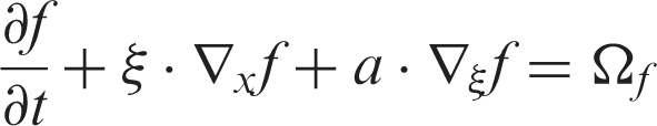
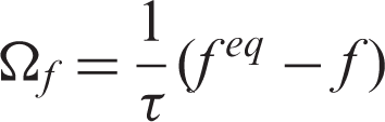
The collision operator involves nonlinear integral, which makes the computation rather complicated. With the aid of Bhatnagar–Gross–Krook (BGK) approximation, the lattice Boltzmann equation (LBE) can be significantly simplified via replacing the collision operator with linearized expression. Since the system will finally reach the equilibrium state, the distribution function f tends to approach the Maxwell distribution function $f^{\mathit{eq}}$ . Through single-relaxation-time approximation, the collision operator takes the following form

$${\Omega }_f=\frac{1}{\tau }(f^{\mathit{eq}}-f)$$

where τ is a dimensionless parameter representing the relaxation time.

By means of discretization in the velocity, space and time, the LBE can be attained

$$f_i(x+c_i\delta t,t+\delta t)-f_i(x,t)={\Omega }_i(x,t)+F_i(x,t)$$

where i represents the discrete velocity direction and $f_i(x,t)$ is the particle distribution function along the direction of $c_i$ . The position is defined as a square lattice in space, with lattice spacing $\delta x=c_i\delta t$ , while the time is separated with time step, $\delta t$ . The space and time resolution $\delta x,\delta t$ can be specified in any set of units. The widely adopted choice is the lattice unit, which is dimensionless with $\delta x^{*}=\delta t^{*}=1$ (* indicates lattice unit). The quantities can be easily converted between physical units and lattice units via conversion factor. More details can be found in Krüger et al. ³ Considering the laws of similarity, we can focus on the dimensionless number like Reynolds number in the simulation.

As the most popular LBE method, the lattice Boltzmann equation with BGK approximation (LBGK) has been widely applied in a variety of complex flows.

$$f_i(x+c_i\delta t,t+\delta t)-f_i(x,t)=\frac{1}{\tau }({f_i}^{\mathit{eq}}-f_i)+F_i(x,t)$$

The main process of calculation can be divided into two steps. One is the relaxation/collision step, which implements collision in the local lattice site. The other is the streaming/propagation step, which indicates the movement of particles towards neighboring lattice sites. Apparently, the first step only involves local calculation and the second step only requires next neighbor interaction. Therefore, the LBM is naturally suitable for parallel computation on GPUs.

$$\text{Relaxation}:{f_i}^{*}(x,t)=f_i(x,t)+\frac{1}{\tau }({f_i}^{\mathit{eq}}-f_i)+F_i(x,t)$$

$$\text{Streaming}:f_i(x+c_i\delta t,t+\delta t)={f_i}^{*}(x,t)$$

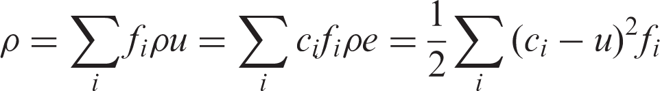
The macroscopic parameters such as density, velocity and internal energy can be calculated statistically from moments of the discrete distribution function.

$$\rho =\sum _i{f}_i\rho u=\sum _i{c}_i{f}_i\rho e=\frac{1}{2}\sum _i{(c_i-u)}^2{f}_i$$

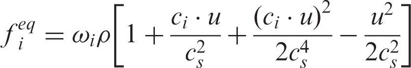
In the prevailing DdQm discretization model, where d denotes the number of dimensions and m is the number of velocity sets, the equilibrium distribution function can be described as follows

$$f_i^{\mathit{eq}}={\omega }_i\rho [1+\frac{c_i·u}{c_s^2}+\frac{{(c_i·u)}^2}{2c_s^4}-\frac{u^2}{2c_s^2}]$$

where ${\omega }_i$ is the weight associated with velocity set and $c_s$ is the sound speed depending on the chosen lattice model. In this paper, the prevailing D2Q9 model is selected in two-dimensional simulation, where the distribution functions are labeled in the light of their direction (rest, east, north, west, south, northeast, northwest, southwest, southeast) as $f_r,f_e,f_n,f_w,f_s,f_{\mathit{ne}},f_{\mathit{nw}},f_{\mathit{sw}},f_{\mathit{se}}$ .

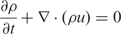
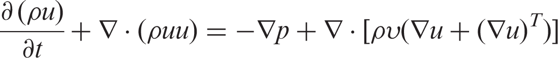
By virtue of the multi-scale analysis method called Chapman-Enskog expansion, the hydrodynamic equations corresponding to the LBGK model can be obtained

$$\frac{\partial \rho }{\partial t}+\nabla ·(\rho u)=0$$

$$\frac{\partial (\rho u)}{\partial t}+\nabla ·(\rho \mathit{uu})=-\nabla p+\nabla ·[\rho \upsilon (\nabla u+(\nabla u{)}^T)]$$

where $\nu =c_s^2(\tau -0.5)\delta t$ , which is the kinematic viscosity. Under the limitation of small Mach number, the variation of density can be neglected. Thus, the above equations can recover incompressible Navier-Stokes equations at the macroscopic scale. ⁴

In view of multiphase fluid, there are mainly four types of LBE models, including color-gradient model, pseudo-potential model, free energy model and LBE models based on kinetic theories. Among the mentioned models, Shan–Chen model has attracted wide attention due to its simplicity and effectiveness. This model owes its name to Shan and Chen ⁵ who introduced a pseudo-potential and non-local force in order to depict the interaction between fluid particles.

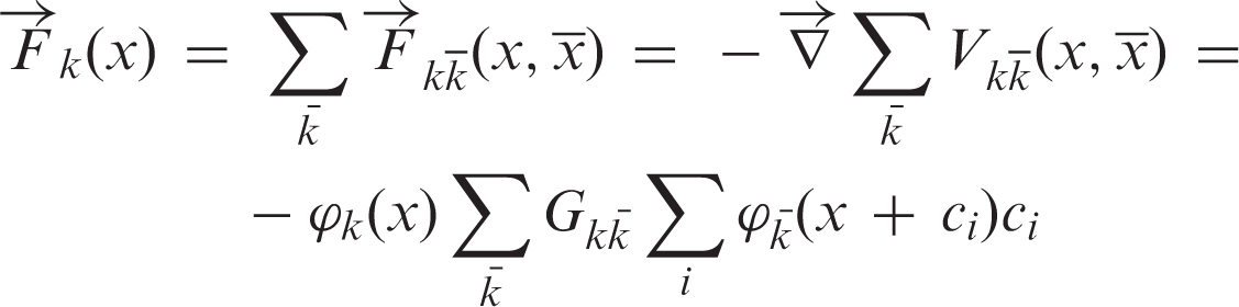
In a multiphase fluid system constituted by n components, the LBE of Shan–Chen model can be expressed as

$$\begin{array}{c}\multicolumn{1}{c}{f_{\mathit{ki}}(x+e,t+\Delta t)-f_{\mathit{ki}}(x,t)=-\frac{1}{{\tau }_k}(f_{\mathit{ki}}(x,t)-{f_{\mathit{ki}}}^{\mathit{eq}}(x,t)),k=1,\dots n}\end{array}$$

where $f_{\mathit{ki}}$ , ${f_{\mathit{ki}}}^{\mathit{eq}}$ , ${\tau }_k$ is the distribution function, equilibrium distribution function and relaxation time of the k component.

The pseudo-potential between different phases takes the following form

$$V_{k\overline{k}}(x,\overline{x})=G_{k\overline{k}}(x,\overline{x}){\varphi }_k(x){\varphi }_{\overline{k}}(\overline{x})$$

where $G_{k\overline{k}}$ is a Green function to determine the strength and range of interaction between k and $\overline{k}$ component, and ${\varphi }_k$ denotes the effective density of the k component and is proportional to the effective mass. The total interaction force acting on the k component can be computed by adding the force imposed by all the rest components.

$${\overrightarrow{F}}_k\left(x\right)\text{=}{\displaystyle \sum _{\overline{k}}{\overrightarrow{F}}_{k\overline{k}}\left(x,\overline{x}\right)}=-\overrightarrow{\nabla }{\displaystyle \sum _{\overline{k}}{V}_{k\overline{k}}\left(x,\overline{x}\right)}\text{=}-{\phi }_k(x){\displaystyle \sum _{\overline{k}}{G}_{k\overline{k}}}{\displaystyle \sum _i{\phi }_{\overline{k}}}(x+c_i)c_i$$

The Shan–Chen model does not need any explicit interface tracking because the macroscopic separation and interface between multiphase naturally emerges from microscopic interactions between different fluid components, which brings convenience and flexibility. Compared with other models, Shan–Chen model has satisfactory performance in both efficiency and accuracy. Thus, it is adopted in the multiphase LBM simulation.

Fundamentals of GPU and CUDA

Since the NVIDIA Corporation introduced the GPU with CUDA architecture, an increasing number of applications have witnessed desirable acceleration with the aid of parallel computation. As a parallel computing platform and programming model invented by NVIDIA, CUDA has enabled a straightforward implementation of parallel algorithms and leads to dramatic increases in computing performance. Programmers can concentrate on the task of parallelization of the algorithms rather than wasting time on the details of implementation.

In the CUDA programming model, the heterogeneous computation model is adopted. The CPU is assumed as host, and GPU is viewed as a device that is capable of executing a quantity of threads in parallel. The parallel portions of computation will be allocated to the GPU, while serial portions of applications are run on the CPU. The CPU and GPU are treated as separate devices with their own host memory and device memory. This configuration allows simultaneous computation on the CPU and GPU without conflicts on memory resources.

The CUDA-enabled GPU with multilevel memory architecture and multi-threads parallel computation method facilitates the computation with more flexibility. GPU is composed of several streaming multiprocessors (SM), each including a set of scalar processors (SP). The main storage consists of a large off-chip device memory, which is optimally divided into global, constant and texture memory. The global memory is sufficient but suffers from high latency. The constant and texture memory are especially designed for read-only data and specific data formats. Every SM also provides the SPs with local registers and on-chip shared memory that allows communication within an SP with much higher bandwidth and lower latency.

The functions in programming are called kernels which are executed N times in parallel by N different CUDA threads. Each thread has its private memory such as local register. The threads will be batched together into thread blocks in a one-dimensional, two-dimensional or three-dimensional form. All threads of a block will reside on the same processor core and share the limited memory resources, which imposes a limit on the maximum number of threads per block. Each thread block has shared memory merely visible to threads within the block. Threads in the same block can cooperate by sharing data through fast shared memory and synchronizing the execution to coordinate memory accesses. Then, blocks will be organized into a one-dimensional, two-dimensional or three-dimensional grid. This hierarchy brings about convenience when invoking computation across the elements in vector, matrix or volume. Threads indifferent thread blocks from the same grid cannot synchronize and communicate with each other. However, all threads have access to the same global, constant and texture memory. ⁶

The compute node is equipped with 2 CPU (Inter Xeon E5-2630v3) cores (32 hyper threaded cores) and a NVIDIA Tesla K20 GPU, which contains a total of 2496 processor cores and is equipped with 5 GB of on-board memory, with memory bandwidth up to 208 GB/s. The Tesla K20 delivers 1.17TFlops (floating point performance) peak double-precision performance and 3.52 TFlops peak single-precision performance, which can provide high throughput for the demanding high-performance computing.

Implementation of LBM on GPU

With the fundamental knowledge of architecture of GPU and CUDA, we will then focus on implementation of LBM on GPU. The methods put forward by Tölke^7,8 that take advantage of shared memory to accelerate have been widely acknowledged and utilized, which is adopted in this paper.

There are mainly four kernels to achieve LBM in CUDA. The first kernel is LBCollProp, which deals with collision and propagation. The two steps are merged in one kernel to enhance the efficiency of memory access. Considering a two-dimensional grid size of NX×NY, the block is defined as (threads_num, 1, 1) and the grid is set as (NX/threads_num, NY, 1), where threads_num is the number of threads per block in X direction. Within each block, the distribution functions first execute the collision, which only contains calculation in the local node. Then, the distribution functions of $f_r$ which rests and $f_n,f_s$ which move along Y direction can be directly written to the device memory due to alignment of location in memory. However, the rest distribution functions which shift along X direction require extra attention. It is recommended to use the shared memory in the block to propagate and then write back to device memory without a shift.

The second kernel is LBExchange, which is responsible for exchanging distribution functions across the borders of the thread blocks. Because shared memory is only accessible to threads in the same block, the distribution functions on borders of blocks will be temporarily stored at the opposite side in the first kernel. In this kernel, every row is processed in sequence along X direction to put the distribution functions on the border in the appropriate location. There are two loops that will separately move $f_w,f_{\mathit{nw}},f_{\mathit{sw}}$ to the west and move $f_e,f_{\mathit{ne}},f_{\mathit{se}}$ to the east. It needs to be shifted under a certain order to avoid overwriting data. Since the procession of different rows is independent, the block is set as (threads_num, 1, 1) and the grid is defined as (1, NY/threads_num, 1). Consequently, the distribution functions can propagate to the correct position after collision.

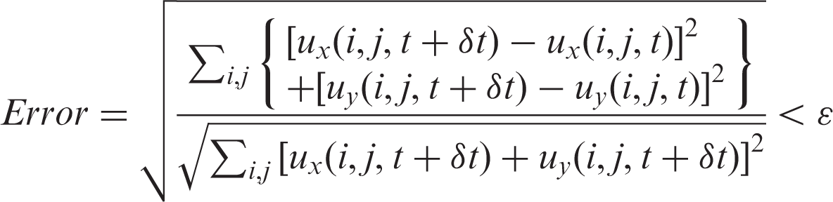
The third kernel is LBBoundary that fulfills the boundary conditions. The configuration is the same as the second kernel. The fourth kernel is LBError, which calculates the relative error of the fluid field. Actually, it can be deemed as the procedure of reduction that adds up the error. The implementation is optimized to reduce thread divergence according to the method introduced by Kirk et al. ⁹

Validation

Two-dimensional lid-driven cavity flow

Since the lid-driven cavity flow presents various vortex motions, it is analyzed to validate the two-dimensional LBM and to compare the performance between implementation on CPU and GPU. In terms of the CPU code, we refer to the sample code provided by He et al. ¹⁰ in C+ + language. As for GPU code, we accomplish the program in CUDA C language. In the CPU and GPU programs, we both choose the double-precision mode to ensure the accuracy. Before the convergence, the output procedure is skipped to avoid the influence of writing data on computing time. The convergence criterion for the velocity field is according to the criterion proposed by He et al. ¹⁰ and ɛ is set at 10⁻⁶.

$$\mathit{Error}=\sqrt{\frac{\sum _{i,j}\{\begin{array}{c}{[u_x(i,j,t+\delta t)-u_x(i,j,t)]}^2\\ +{[u_y(i,j,t+\delta t)-u_y(i,j,t)]}^2\end{array}\}}{\sqrt{\sum _{i,j}{[u_x(i,j,t+\delta t)+u_y(i,j,t+\delta t)]}^2}}}<\varepsilon$$

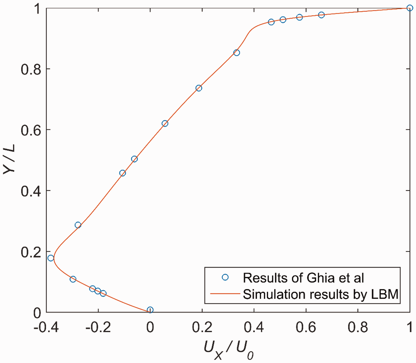
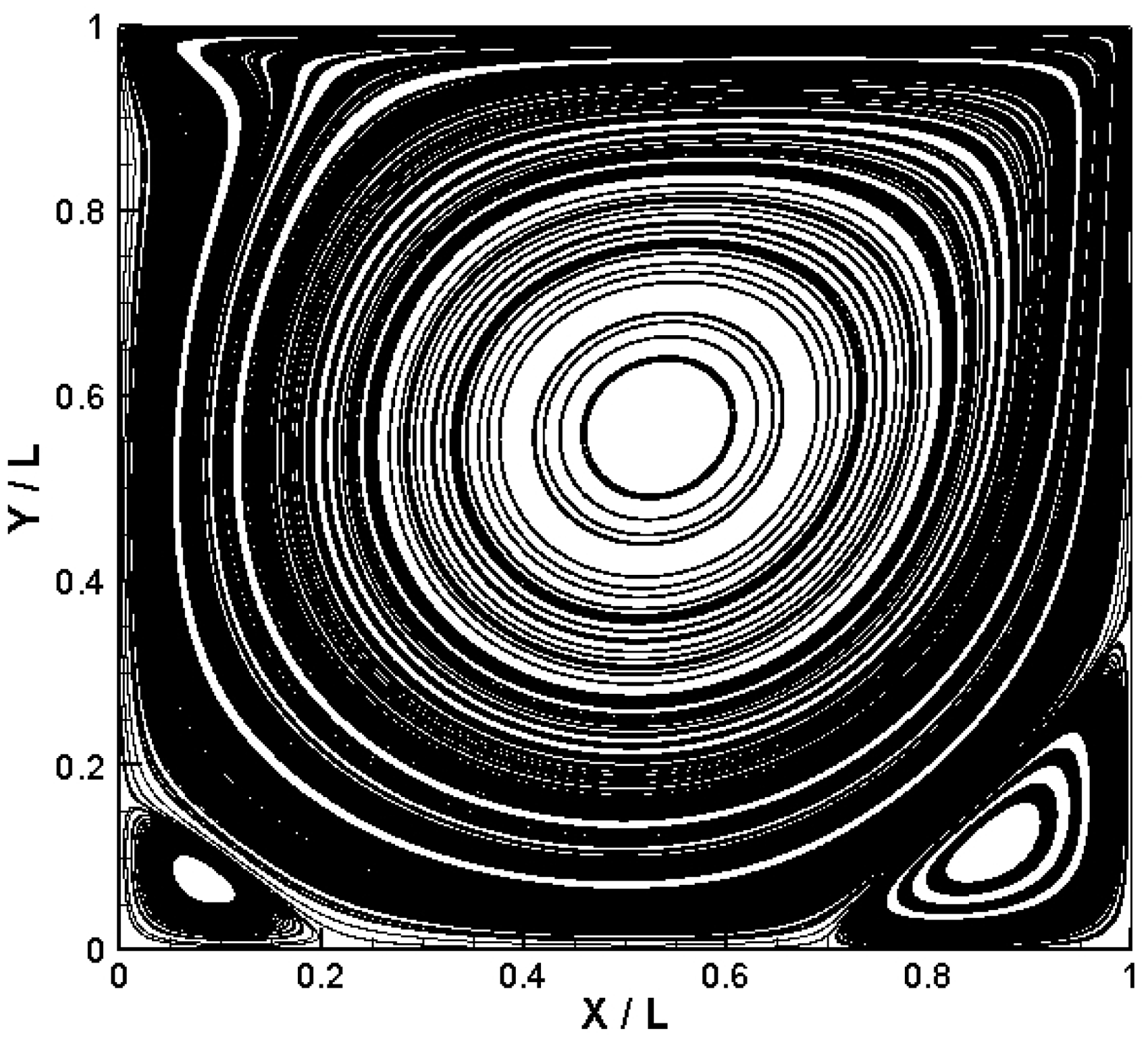
The results of velocity profile through the geometric center of the cavity using GPU are shown in Figures 1 and 2, which are in accordance with the previous benchmark data by Ghia et al. ¹¹ The stream function of the cavity flow with Reynolds number set at 1000 is shown in Figure 3. As is illustrated from the streamlines, a large primary vortex in the center and two secondary vortices near the two lower corners can be observed.

Figure 1.

The velocity profiles of V_y/U₀ through the geometric center of the cavity.

Figure 2.

The velocity profiles of U_x/U₀ through the geometric center of the cavity.

Figure 3.

The streamline for two-dimensional lid-driven cavity flow at Re = 1000.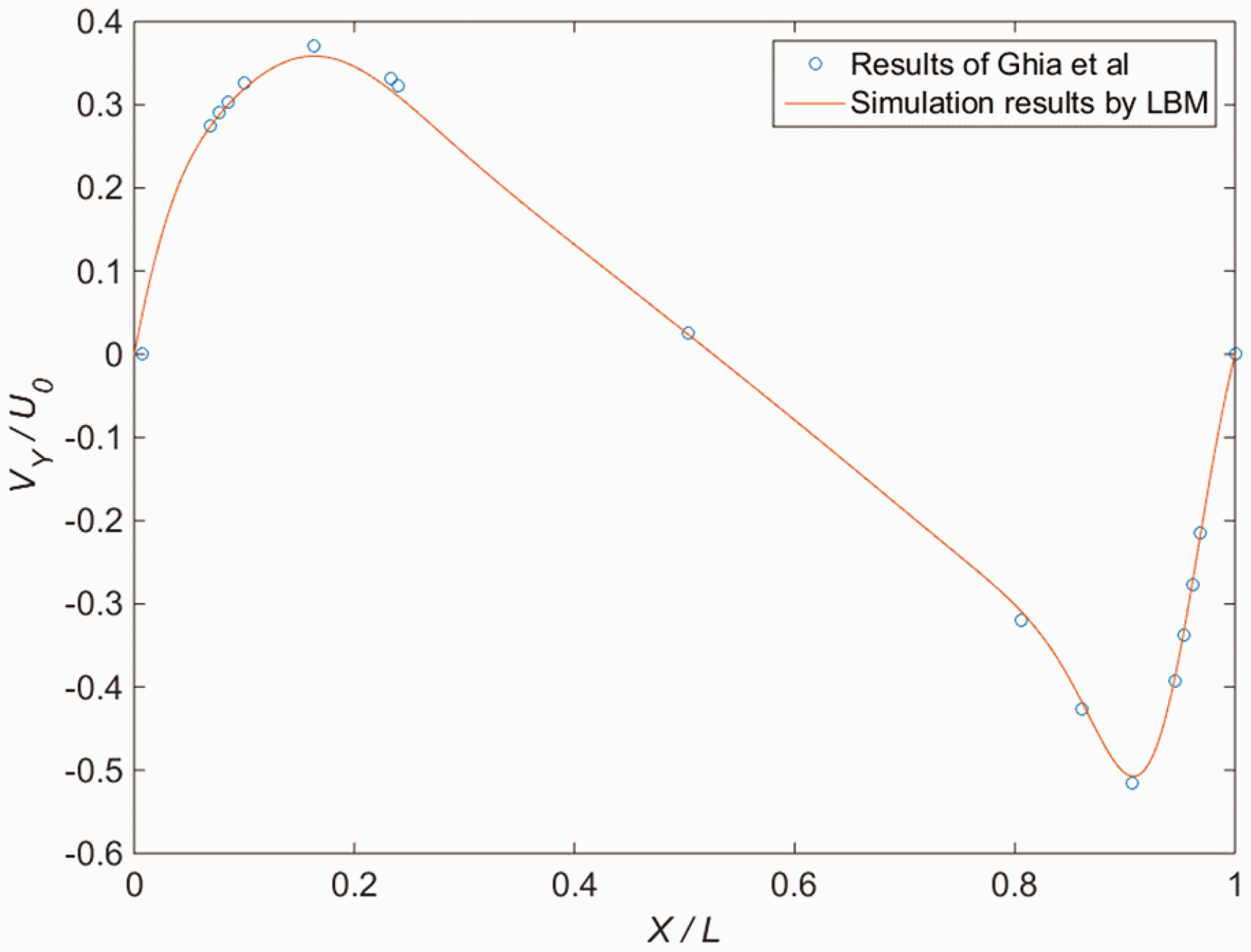

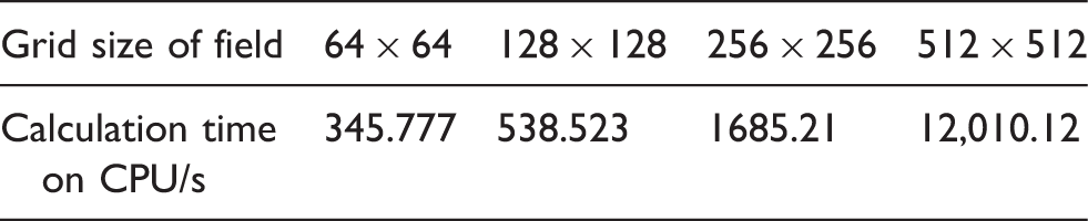
The time for calculation of the same case implemented on CPU and GPU is compared with different grid sizes of fluid field and varying threads per block. The results are shown in the Tables 1 to 3.

Table 1.

Calculation time on CPU with varying grid size of field.

Grid size of field	64 × 64	128 × 128	256 × 256	512 × 512
Calculation time on CPU/s	345.777	538.523	1685.21	12,010.12

Table 2

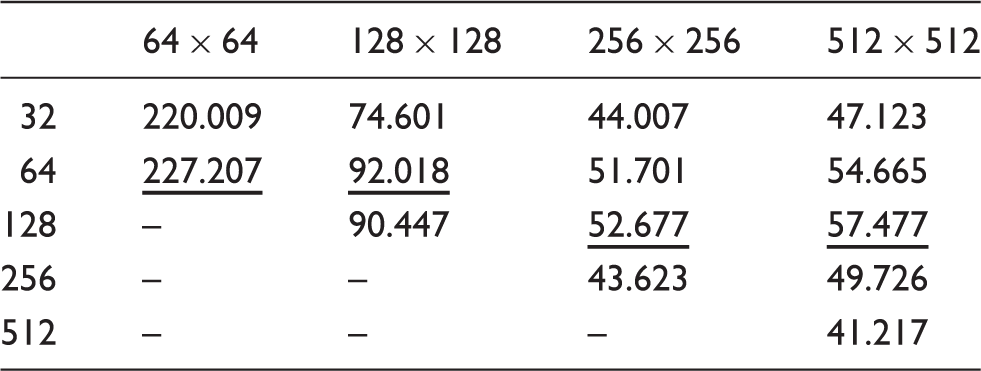
Calculation time on GPU with different grid size of field and varying threads per block.

	64 × 64	128 × 128	256 × 256	512 × 512
32	1.572	7.219	38.295	254.868
64	1.522	5.852	32.596	219.702
128	–	5.954	31.992	208.954
256	–	–	38.631	241.526
512	–	–	–	291.385

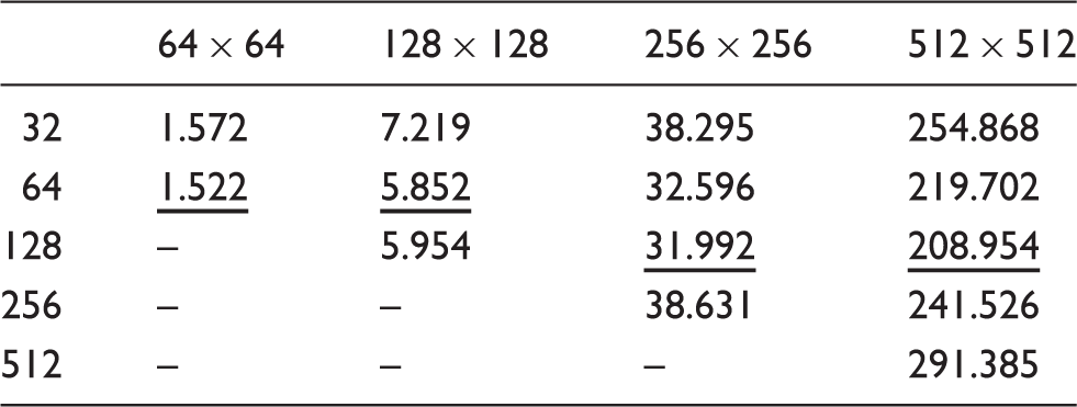
Note: The underlined ones are the minimum calculation time with a specified grid size.

Table 3.

Acceleration ratio with different grid size of field and varying threads per block.

	64 × 64	128 × 128	256 × 256	512 × 512
32	220.009	74.601	44.007	47.123
64	227.207	92.018	51.701	54.665
128	–	90.447	52.677	57.477
256	–	–	43.623	49.726
512	–	–	–	41.217

Note: The underlined ones are the maximum acceleration ratio with a specified grid size.

With a certain grid size, the minimum calculation time and the maximum acceleration ratio are underlined, which are associated with an appropriate number of threads per block. The acceleration ratio is rather desirable on the whole, which shows the distinct competitiveness of GPU over CPU in the implementation of LBM.

Two-dimensional fully developed laminar Poiseuille flow

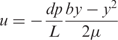
The two-dimensional fully developed laminar Poiseuille flow can be considered as the fluid flow through two parallel infinite plates. The theoretical solution will be discussed in detail. The velocity profile can be described as the following formula

$$u=-\frac{\mathit{dp}}{L}\frac{\mathit{by}-y^2}{2\mu }$$

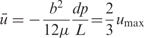
The mean velocity of the cross section is

$$\overline{u}=-\frac{b^2}{12\mu }\frac{\mathit{dp}}{L}=\frac{2}{3}{u}_{max}$$

The pressure drop along the path is

$$\mathit{dp}=f\frac{l}{d}\frac{\rho {\overline{u}}^2}{2}=\frac{24}{\text{Re}}\frac{L}{b}\frac{\rho {\overline{u}}^2}{2}$$

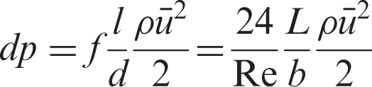
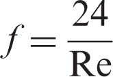
The Darcy friction factor can be derived from the above analysis

$$f=\frac{24}{\text{Re}}$$

A fully developed parabolic velocity profile is prescribed at the inflow, and a constant pressure condition is prescribed at the outflow for all test cases. The length of the tube is chosen to be long enough to alleviate errors caused by the influence of inlet and outlet region. The simulation data for the analysis of the pressure drop of Poiseuille flow are shown in the Table 4 and Figure 4. The slope of linear fit line through the data is 23.76 with coefficient of determination close to one, which is in satisfactory agreement with the theoretical result. The results prove the effectiveness of the model to simulate fluid pipe flow.

Table 4.

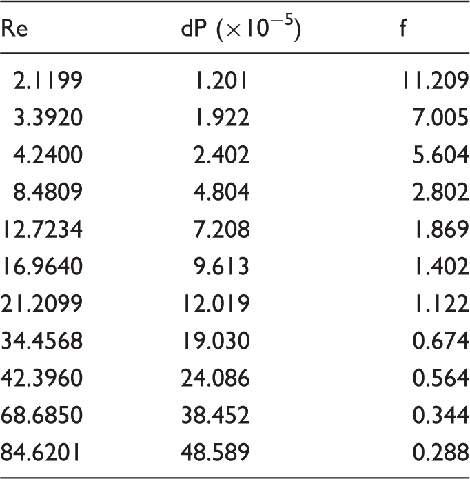
The data of pressure drop and friction factor with varying Reynolds number.

Re	dP (×10−5)	f
2.1199	1.201	11.209
3.3920	1.922	7.005
4.2400	2.402	5.604
8.4809	4.804	2.802
12.7234	7.208	1.869
16.9640	9.613	1.402
21.2099	12.019	1.122
34.4568	19.030	0.674
42.3960	24.086	0.564
68.6850	38.452	0.344
84.6201	48.589	0.288

Figure 4.

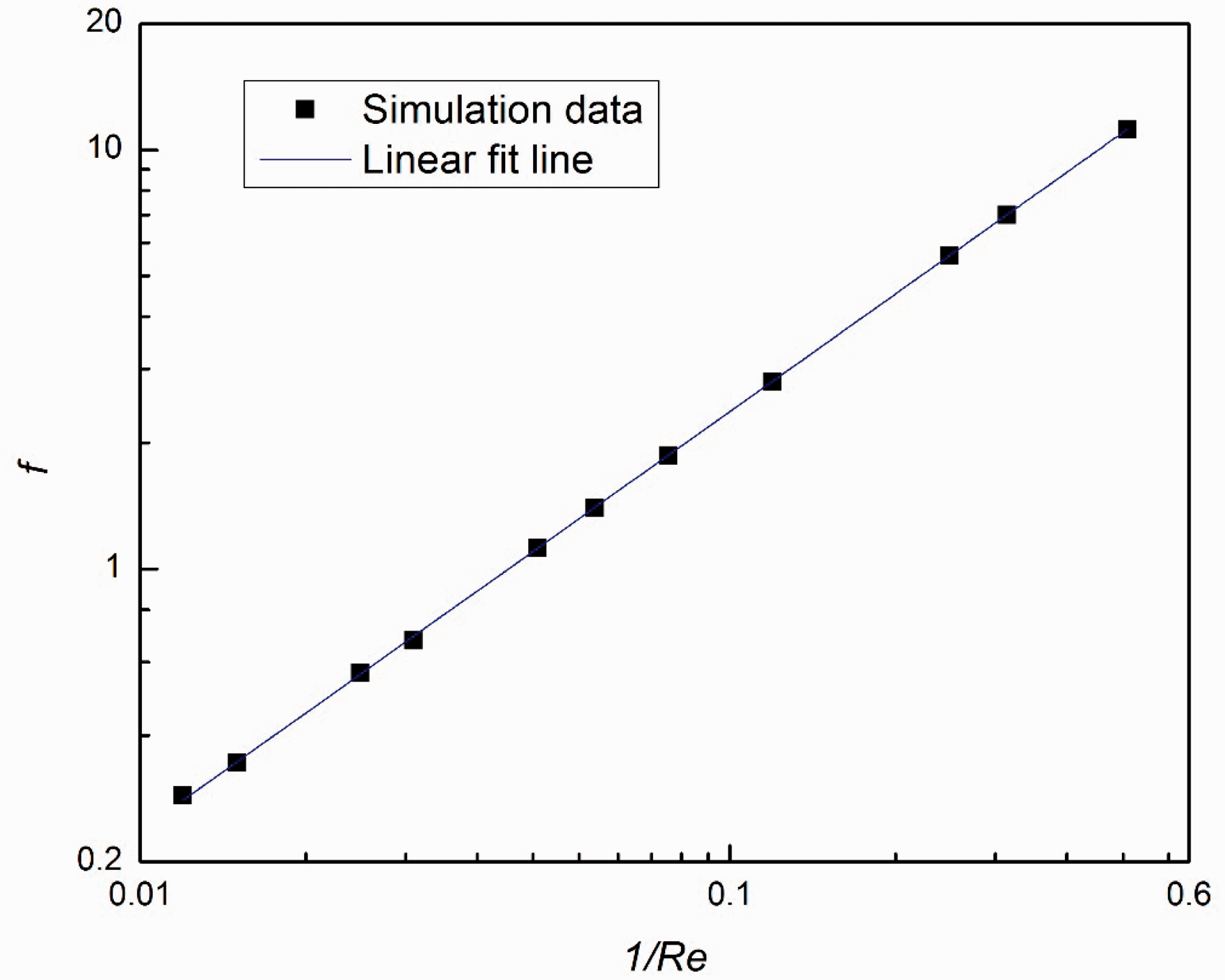
The linear fit line of Darcy friction factor with varying Reynolds number in logarithmic coordinates.

Validation of Laplace Law

In order to validate the Shan–Chen multiphase model, the Laplace Law is employed to evaluate the surface tension for droplets in equilibrium, which is defined in the following formula

$$\Delta p=\frac{\sigma }{R}$$

where σ represents the surface tension and R is the radius of the droplet. The pressure difference is calculated through the subtraction of pressure inside and outside the droplet.

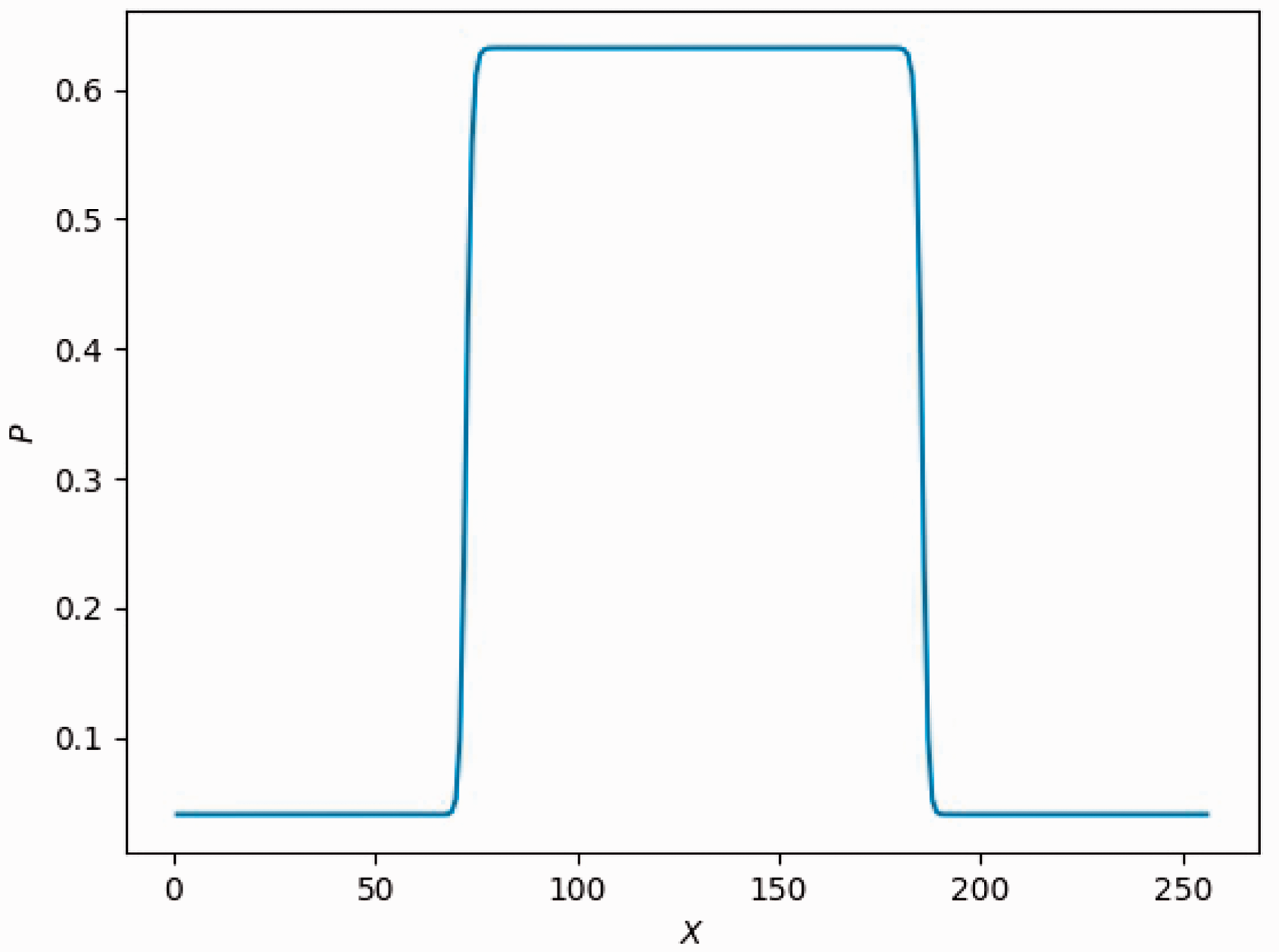
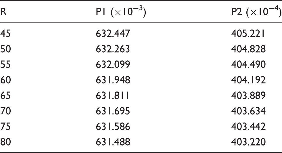
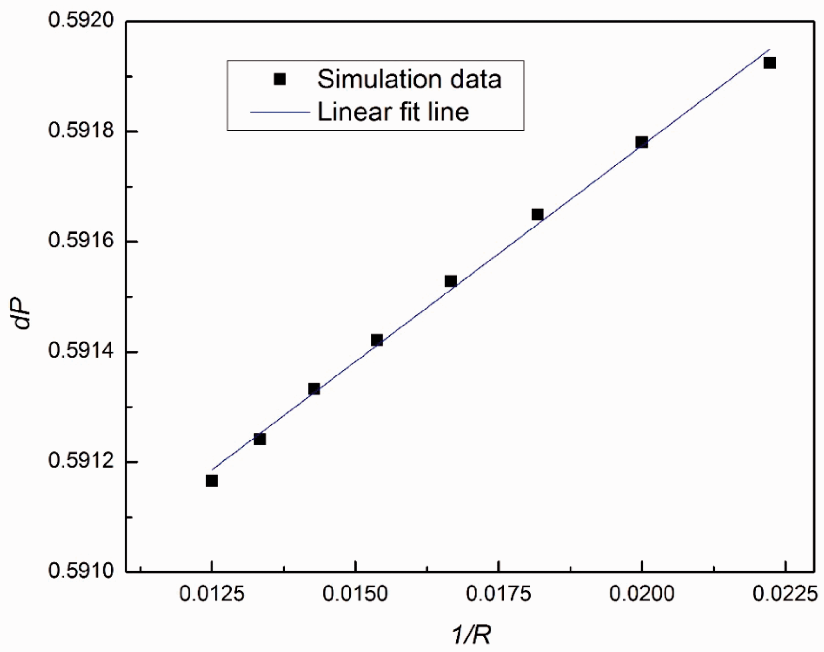
In this case, the computational domain consists of 256 × 256 lattice nodes. The boundaries are all periodic. A static droplet is initially posed in the center of the field as indicated in Figure 5. The computation is set at double-precision mode, and the pressure difference is shown in Figure 6 and Table 5. As manifested in Figure 7, the results show satisfactory linearity between the pressure difference and the reciprocal of radius with coefficient of determination above 0.99, which is in desirable agreement of the Laplace Law.

Figure 5.

The density field of the droplet.

Figure 6.

The pressure variation along horizontal centerline.

Table 5.

The pressure inside (P1) and outside (P2) the droplet with varying radius.

R	P1 (×10−3)	P2 (×10−4)
45	632.447	405.221
50	632.263	404.828
55	632.099	404.490
60	631.948	404.192
65	631.811	403.889
70	631.695	403.634
75	631.586	403.442
80	631.488	403.220

Figure 7.

The pressure difference versus reciprocal of radius.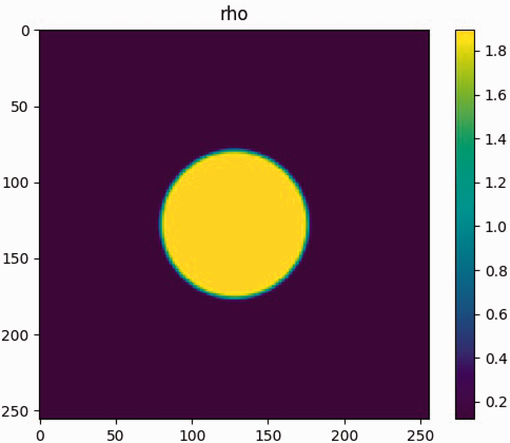

Demonstrative results and discussion

In this section, we will firstly study the two-dimensional multiphase fluid pipe flow in vertical tube under gravity with vertical periodic boundary condition. Then, we will explore the two-dimensional multiphase fluid pipe flow in horizontal tube under gravity and horizontal force with horizontal periodic boundary condition.

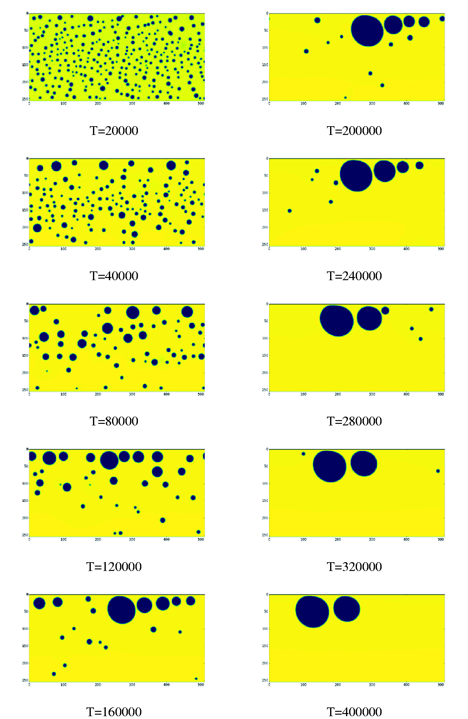
Initially, the density of the fluid field is randomly set up at higher or lower value. Under the effect of interphase force, the bubbles gradually collide and coalesce into bigger ones. At the same time, the bubbles and fluids are accelerated by the external force such as gravity or horizontal force. The gravity acceleration is set at 10⁻⁵ and the horizontal force is set at 10⁻⁶. The simulation results at different time steps are shown in Figures 8 and 9. The dark area represents the lower density bubbles, while the yellow area stands for the higher density fluid.

Figure 8.

Density field of vertical tube at different simulation steps.

Figure 9.

Density field of horizontal tube at different simulation steps.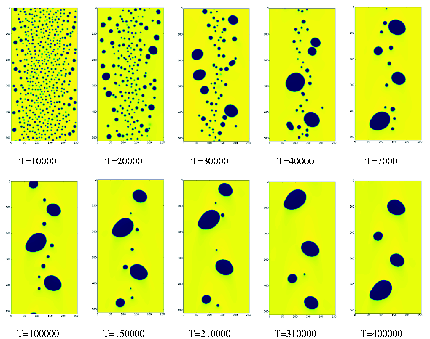

Vertical tube

In the initial stage, the bubbles distribute uniformly in the field (T = 10,000). Because the velocity near the wall is smaller than the center and wall shear stress is larger than the center, the bubbles near the wall are likely to collide with each other and gradually coalesce into bigger ones. At the same time, the bubbles in the center of tube moves faster and remain relatively small (T = 20,000). After a period of collision, the bubbles near the wall merge into medium ones and the number of bubble decreases distinctly. The distribution of bubbles appears to be smaller and more in the center, while bigger and less near the wall (T = 30,000). Because the velocity in the center of tube is higher than near the wall, the big bubbles gradually move towards the center under the impact of high-speed fluid. This process contributes to the mixture of big bubbles near the wall and small bubbles in the center (T = 40,000). Gradually, the domain of small bubbles shrinks and the number of bubble declines. With the fusion of bubbles, the size of big bubbles is on the increase. In the meanwhile, the shape of big bubbles deforms and deviates from circle, which appears a variety of shapes including, ellipse, rectangular, triangular, etc. (T = 70,000). Then, all bubbles gather in the center of tube, where the velocity is larger. By contrast, there exist barely any bubbles near the wall. The big bubbles and small bubbles appear to be intermittent and compatible in the process of simulation (T = 150,000). Finally, the small bubbles merge into the big ones and only some major elliptic bubbles exist (T = 400,000).

Horizontal tube

Similar to the vertical tube, the bubbles distribute uniformly in the field initially (T = 20,000) and gradually forms bigger bubbles near the wall, while the bubbles in the center of tube retain relatively small (T = 40,000). Later on, the bigger bubbles in the upper layer approach the wall of tube and only move in horizontal direction, while the bigger bubbles in the bottom layer rise under the effect of buoyancy force. When they go up and pass the center of tube, they encounter with the small bubbles and enhance mixture and coalescence (T = 80,000). Owing to the rising bubbles, the number of small bubbles decreases, while the number of intermediate bubbles increases. Afterwards, the bigger bubbles rise to the upper layer of tube sooner or later (T = 120,000). If they meet up with the previous big bubbles, a relatively huge bubble will be formed (T = 160,000). With the size of bubble increasing, there exists a bit of deformation of the shape of bubble and deviation from circle. At the same time, only few smaller bubbles exist in the lower domain (T = 200,000). Under the effect of horizontal force, the bubbles in the upper layer moves in horizontal direction, which promotes the medium-size bubble to collide and grow into bigger ones. An interesting phenomenon is that during the merging process, several bubbles exist very close to each other, and the size of bubbles is increasing one by one against the direction of horizontal force. The smaller bubbles move at the front while the bigger bubbles move at the end. This distribution remains stable for awhile. Even after some procedures of collision and aggregation into bigger bubbles, this distribution pattern is reproduced once again (T = 240,000). It demonstrates that this distribution is balanced under the effect of gravity and horizontal force. Then, the bubbles between the fore and tail bubbles first fuse into a big bubble (T = 280,000). Then, it incorporates the small bubble at the front (T = 320,000). Finally, the tiny bubbles join the two big bubbles and they maintain steady movement with some distance between each other (T = 400,000).

Conclusion

In summary, the LBM proves to be an innovative and promising tool for complex fluid flow compared with the traditional CFD methods. The implementation of LBM on GPU delivers satisfactory performance and manifests a notable advantage over CPU. We have accomplished the GPU code in CUDA and carried out the validation cases for the 2D lid-driven cavity flow, 2D steady Poiseuille flow, and the Laplace Law, which is in acceptable accordance with the benchmark results. We also make use of the program to conduct numerical simulations on multiphase flow in vertical and horizontal pipes. The results indicate the effectiveness and efficiency of the LBM on GPU in simulating multiphase flow.