A runtime based comparison of highly tuned lattice Boltzmann and finite difference solvers

Abstract

The aim of this work is a fair and unbiased comparison of a lattice Boltzmann method (LBM) against a finite difference method (FDM) for the simulation of fluid flows. Rather than reporting metrics such as floating point operation rates or memory throughput, our work considers the engineering quest of reaching a desired solution quality with the least computational effort. The specific lattice Boltzmann and finite difference methods selected here are of a very basic nature to emphasize the influence of the fundamentally different approaches. To minimize the skew in the measurements, complex boundary condition schemes and further advanced techniques are avoided and instead both methods are fully explicit, weakly compressible approaches. Due to the highly optimized nature of both codes, different sets of restrictions are imposed by either method. Using the common set of features, two relatively simple test cases in terms of a duct flow and the flow in a lid driven cavity are considered and are tuned to perform optimally with both approaches. As a third test case, a transient flow around a square cylinder is used to demonstrate the applicability to engineering oriented settings and in a temporal domain. The performance of the two methods is found to be very similar with no full advantage for any of the approaches. Overall a tendency toward better performance of the LBM at larger target errors and for indirect benchmark quantities, such as lift and drag, is observed, while the FDM excels at smaller target errors and direct comparisons of velocity and pressure profiles to analytical solutions. Other factors such as the difficulty of setting consistent boundary conditions in the LBM or the effect of stabilization in the FDM are likely to be the most important criteria when searching for a very fast flow solver for practical applications.

1. Introduction

In this work, we assess performance aspects of the lattice Boltzmann method (LBM) and the finite difference method (FDM) in solving the incompressible Navier–Stokes equations (NSE). The LBM has gained much popularity in recent years and is well-known for its high performance. It has been used successfully in a variety of applications, such as external car aerodynamics or biological flows (Aono et al., 2010; Duncan et al., 2010; Krafczyk et al., 1998; Lockard et al., 2000). There are two potential reasons for the high performance of the lattice Boltzmann implementations. On the one hand, it can be due to advantageous features of the method itself, rooting in the gas-kinetic origin. On the other hand, the limited features set common to many implementations, such as globally uniform rectangular grids, might allow for a much more efficient implementation of the algorithms. This raises the question whether traditional continuum-based approaches can reach the same level of performance or even surpass them in case the method is restricted to a similar feature set.

Previous research involving comparison of the lattice Boltzmann method covers a wide field of topics. The publications by Noble et al. (1996), Bernsdorf et al. (1999), Kandhai et al. (1999), He et al. (2002), Marié et al. (2009) as well as Ohwada et al. (2011) are concerned with convergence orders and achievable error for a wide range of methods and applications. Naturally, the results depend directly on the particular variant of the employed methods and are snapshots of the wide field of possible combinations and applications. The research by Junk (2001) and Holdych et al. (2004) is more general in the sense that they establish the mathematical relationship between selected versions of the LBM and a finite difference stencil counterpart. However, these do not allow for conclusions in terms of solution quality per runtime, as a difference in throughput between the methods can dramatically change the outcome of the comparison. The publications by Yoshino et al. (2004) and Geller et al. (2006) include timing information, which allows to introspect the performance for the specific implementations and test case to be evaluated. The chosen approaches can be quite heterogeneous and the research was not tailored explicitly toward performance in runtime. The goal of this publication is to fill this gap by stringently aligning all parameters toward an unbiased comparison in terms of total runtime. The focus lies on distinguishing the influence of the underlying approaches from surrounding factors such as simulation setup and code tuning. To this end, the compared methods are reduced to the bare essentials omitting complex techniques and keeping methods as similar as possible. The test case selection also adheres to this concept and they are chosen to be simple, equally suitable for both methods and enable a clear quantification of the result quality. These directly quantifiable test cases are supplemented by a further test which introduces transient behavior and more complex flow patterns.

With the lattice Boltzmann method representing one side of this comparison, the classical approach to solving the NSE is represented by a finite difference method. It has a very rich history of high performance computations (Kim and Sandberg, 2012) and countless fields of application. Each code has been extensively tuned specifically for the used platform to ensure a fair comparison at the highest performance levels.

Despite the widely different approach of the LBM compared to traditional NSE solvers, there are many similarities between the LBM and the FDM (He et al., 2002). In fact, FD stencils can be derived from collision operators of the LBM (Holdych et al., 2004; Junk, 2001). Furthermore, both approaches show similarities in accuracy and convergence behavior (Geller et al., 2006; He et al., 2002; Marié et al., 2009). It is important to note that for this work the suitability for a fair comparison plays a larger role in the selection of method particularities than their use in practice. However, such a selection comes naturally with common use cases and similar restrictions. In both cases, the domains are discretized using a structured mesh and complex geometries need to be represented through immersed boundary conditions.

Each method on its own already offers innumerable configuration possibilities, such as the type of time integration, spatial order, stabilization, the boundary condition implementation and so on. A direct comparison of every possible configuration of both methods is infeasible. In order to narrow down the number of parameters some design choices have to be made. All restrictions done in this work are carefully selected in order to avoid favoring one method in a disproportionate way. The outcome of this process is described in the sections on the methods and test cases.

Considering the limitations set forth by the methods, two steady-state test cases and a transient test case have been selected. The steady-state duct flow and the non-leaky lid driven cavity (LDC) are set up to ensure fair tests and the simulation and code parameter are optimized for each method to ensure highest performance. The parameters for the transient test case of a flow around a cylinder with square cross section are determined with the aid of a steady-state precursor simulation which are then applied to the full transient version. Even though all test cases consider relatively low Reynolds number flows, the ingredients of the methods explicitly include stabilization mechanism that enable the use also for higher Reynolds numbers and in the turbulent regime. This then leads to direct numerical simulations, which resolve all physically relevant scales, or large eddy simulation in terms of implicit subgrid closures. Of course, explicit subgrid closures could provide even better accuracy for certain configurations (Sagaut, 2006), but no conclusions can be drawn along those directions from the present work.

Furthermore, for the test cases quasi-incompressible fluids are considered. While there is a vast amount of literature regarding the extension to fully compressible flows with higher Mach numbers for both methods, and both methods could indeed be extended toward those computations, a detailed accuracy versus cost comparison has not yet been performed to the best of the authors’ knowledge.

This article is structured as follows: First the LB and FD method with the respective implementations are introduced. Then, some common information on the test cases is given, followed by the test results themselves. The findings are discussed and finally a conclusion is drawn.

2. Methods and implementation

2.1. Lattice Boltzmann method

The lattice Boltzmann method is a rather recent development in the field of computational fluid dynamics (CFD) (Succi, 2001). Its concept is fundamentally different from traditional CFD methods. Instead of discretizing the Navier–Stokes equations, it emerges from a simplified gas-kinetic description as a velocity discrete Boltzmann equation. The Navier–Stokes equations are then approached in the macroscopic limit.

The LBM is often mentioned as reaching very high performance and the performance aspect is a popular field of research (Pohl et al., 2004; Williams et al., 2008, 2009). The code used in this study is a highly tuned implementation and was developed through multiple projects by the International Lattice Boltzmann Development Consortium (ILBDC) (Wittmann et al., 2014; Zeiser et al., 2009a). More precisely, a simple and highly tuned two-relaxation-time (TRT) version of the LBM is used, which circumvents some of the issues with the even more basic single-relaxation-time (SRT) operators and simultaneously avoids the mathematical and code complexity of multiple-relaxation-time (MRT) or non-linear operators.

The Lattice Boltzmann method is based on discretizing the Boltzmann equation. A lattice with constant distances, time steps and hence also velocities is employed on which the density distribution functions are propagated. The typical choice is to non-dimensionalize in such a manner that the lattice site distance and time steps come out to be one and can therefore be eliminated from all equations.

This work chooses a D3Q19 lattice, where D3 denotes the number of space dimensions and Q19 the number of distribution functions (  $f_i,i=0\dots 18$ ). The directions are each tied to constant velocities (c_i) in the directions depicted in Figure 1 and result in a velocity of $c_0=0$ for the central distribution function, a velocity of 1 along the edges and $\sqrt{2}$ for the diagonals. A further relevant velocity is the lattice specific constant speed of sound of $c_s^2=\frac{1}{3}$ , which correlates the macroscopic density $\rho$ and pressure p as $p=c_s^2\rho$ .

Figure 1.

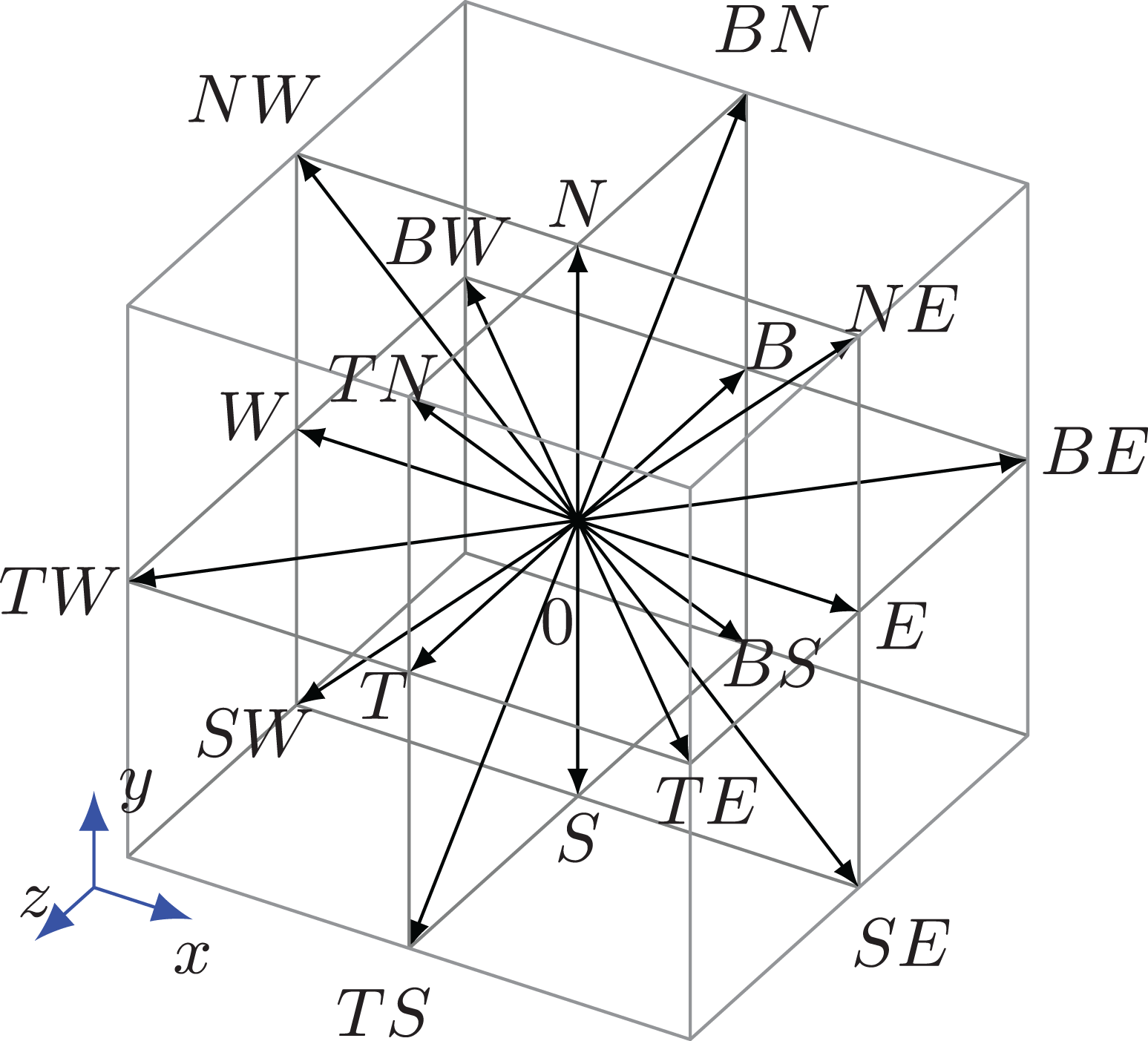
Density distribution functions for a D3Q19 lattice.

The macroscopic density is easily computed as the sum of all density distribution functions per lattice site. Similarly, the momentum at a specific site is merely the sum of the density distribution function times their respective velocities. From this the pressure and velocity fields as the quantities of interest can easily be obtained.

In the LBM the physical behavior is determined by the choice of the collision operator. It is also responsible for most of the computational complexity. The most basic operator is the lattice Bhatnagar–Gross–Krook (LBGK) (Qian et al., 1992) operator, which is a linear single-relaxation-time model. While easy to compute, it has some drawbacks, such as a viscosity that depends on the mesh size. Moreover, the popular midway bounce-back boundary condition is not guaranteed to be exact in between cells (Ginzburg and d’Humières, 2003), and a slow convergence to steady-state solutions has been observed by Pan et al. (2006). To rectify these issues, a two-relaxation-time approach according to Ginzburg et al. (2008a) is implemented.

The collision operations referred to above can be merged with the preceding or the following streaming step into a “pull”- or a “push”-scheme, respectively. For the “pull” approach in conjunction with the selected TRT scheme the full system of equations is

$f_i(x,t+1)=f_i(x-c_i,t)+{\lambda }_e{p}_i+{\lambda }_o{m}_i$

1

$p_i=\frac{1}{2}\left[f_i+f_{\overline{i}}-w_i\left(2c_s^2\rho +3{\left(u\cdot c_i\right)}^2-\parallel u{\parallel }^2\right)\right]$

2

$m_i=\frac{1}{2}\left[f_i-f_{\overline{i}}-2w_i\left(j\cdot c_i\right)\right]\mathrm{.}$

3

The weights w_i are method-specific constants and $\rho$ , u and j are the macroscopic density, velocity and momentum at the current cell location. The symmetric part of the relaxation parameter ${\lambda }_e$ is linked to the viscosity $\nu$ through the relationship

${\lambda }_e=\frac{-2}{6\nu +1},$

4

while the anti-symmetric relaxation parameter ${\lambda }_o$ is a free parameter.

An advantageous choice of the anti-symmetric relaxation parameter is tightly correlated with the type of boundary condition. Boundary conditions are not as straight forward for the LBM as they are for traditional approaches to CFD. For many conditions multiple strategies have been proposed, see e.g. Ansumali and Karlin (2002), Ginzburg et al. (2008a) and Latt et al. (2008). In this work the midway bounce-back (BB) scheme has been selected for no-slip boundaries. It is the simplest in terms of computational complexity and thus exhibits the smallest footprint on the overall simulation duration. Other more advanced approaches may be more robust or offer higher accuracy, but the increase of complexity would shift the focus significantly toward the performance of boundary conditions, which is intentionally not analyzed in more detail here. Additionally, the BB scheme performs quite well for the selected examples, further diminishing the need for other approaches.

For this choice of boundary condition the TRT relaxation parameter for the anti-symmetric component ${\lambda }_o$ can be chosen in such a manner that the boundary interface is exactly at the midway point, which is not generally guaranteed by the BB scheme. The “magic” parameter ${\Lambda }_{eo}=316$ (Ginzburg et al., 2008a) allows ${\lambda }_o$ to be determined as

${\lambda }_o=\frac{2{\lambda }_e+4}{\left(4{\Lambda }_{eo}-1\right){\lambda }_e-2}\mathrm{.}$

5

On the outflow boundaries the pressure is prescribed through the pressure anti-bounce-back (PAB) scheme (Ginzburg et al., 2008b). It is used without any of the additional correction terms.

Typically, the recovery of the Navier–Stokes equations with the lattice Boltzmann method in the asymptotic limit is shown through the Chapman-Enskog expansion (Frisch et al., 1987; Ginzburg et al., 2008b) or by asymptotic analysis (Junk and Yang, 2005; Junk et al., 2005). Convergence orders with respect to the spatial resolution are typically only known for particular setups. For smooth solutions of the linear LBM on periodic domains velocity and pressure are second order accurate (Junk and Yang, 2009). Most commonly however, engineering problems cannot be described using periodic domains. In the case of bounded domains it has been shown that problems using bounce-back implementations yield first order accuracy for the velocity and the pressure is inconsistent (Junk and Yang, 2005). It is important to note that for suitable geometries second order accuracy for velocities and first order accuracy for the pressure can often be achieved, for example by kinetic boundary conditions (Ansumali and Karlin, 2002). Alternative and more complex boundary condition formulations than the BB condition selected for the present work can provide higher accuracy orders, albeit at higher computational cost.

The implementation of this method is highly optimized through several strategies which ensure maximum performance. The code utilizes a Structure of Array (SoA) memory layout to enable vectorization. This layout suffices, as the memory access patterns place a lower load on the number of active memory pages than the FDM code. For example the access to the appropriate density functions of the own fluid cell (for collision) and the neighboring fluid cells (for propagation) are performed through a separate list of connectivity information (Zeiser et al., 2009b). With this approach it is straight forward to merge the collision and propagation into a single loop over the field. The pull-scheme, which is used here, merges the transport toward the collision and subsequent collision (stream-collide) into a single time step. A further advantage of the indirect addressing is that in the context of complex geometries the lattice cells that are not covered by the domain can be skipped altogether. Naturally the index lookups come with the drawback of additional load on the memory interface. Ideally this is minimized by using small data types for addressing, however, the dimensions of the test cases require 64 bit types to enable addressing of all cells.

The ILBDC code is parallelized with OpenMP in a ccNUMA aware fashion. The domain is decomposed according to the number of NUMA domains, which is trivial for rectangular cuboids, and by a linear spacing within the domain. The performance on caching hardware architectures is further increased through a combination of tiling and semi-stencil (de la Cruz and Araya-Polo, 2014) approaches. The complex loop kernel evaluation is split into multiple simpler substeps at lower register pressure. The substeps are then applied sequentially in a spatially blocked fashion, to form the full operation and maximize cache usage at the same time. Additionally the density distribution arrays are toggled between time steps, which eliminates spatial data dependencies and, in conjunction with the pull-scheme, read-for-ownership (RFO) can be eliminated.

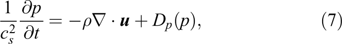
The kernel then requires 175 FLOPS per cell update. For a 28 core dual socket Intel Xeon E5-2690 v4 at 2.6 GHz and with usage of AVX vectorization, this equates to 1664 million cell updates per second (Mupd/s), which is also called lattice site updates (LUP) in the LBM context. The memory bandwidth limit on the aforementioned hardware can be estimated from the required memory footprint per cell evaluation. It is necessary to transfer 152 bytes for reading, 152 bytes for writing (and under many circumstances an additional 152 bytes for RFO) to transfer the density distribution functions. An additional 144 bytes are needed for address lookups due to the indirect addressing. In combination with a measured peak memory bandwidth (BW) of 111.6 GB/s the theoretical throughput is 249 Mupd/s (186 Mupd/s with RFO).

The results of a more advanced estimate than the roofline model, namely the execution cache memory (ECM) model by Treibig and Hager (2010), are provided in Table 1 and also visualized in Figure 2. The measurements in are in good agreement with the memory bandwidth limitation, reaching 87.4% of the theoretical throughput. The diminishing increase of the update rate for larger core counts is also indicative of a memory boundedness.

Figure 2.

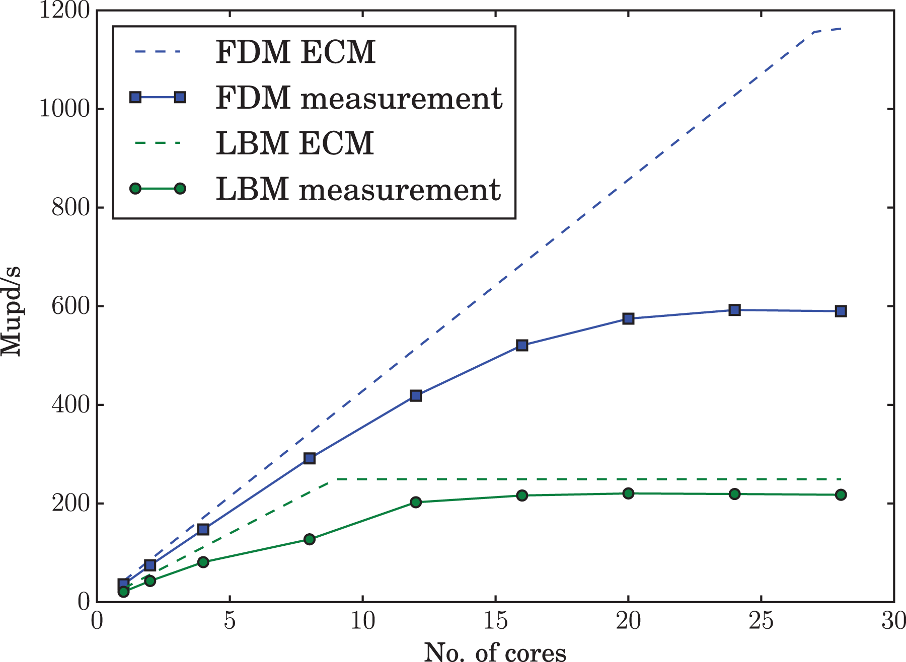
ECM model based and measured performance scaling for the LBM and FDM.

Table 1.

Performance estimate and measurement in Mupd/s of the TRT collision operator in a “pull” scheme without RFO.

No. of cores	1	2	4	8	16	28
Estimated	44.91	89.83	179.66	249.1	249.1	249.1
Measured	20.86	42.86	80.98	127.28	216.15	217.6

It should be noted that the indirect addressing lowers throughput in the bandwidth limited case. In theory, a direct addressing scheme could increase the throughput by up to 47%. However, for a tentative implementation in a structure-of-arrays (SoA) memory layout only a marginally higher (5–15%) throughput was recorded compared to the highly optimized indirect addressing code ILBDC (Wittmann et al., 2014; Zeiser et al., 2009a). The high number of widespread memory locations for 19 arrays that are accessed simultaneously leads to higher latencies and translation-lookaside buffer issues, thereby reducing the effective memory bandwidth. There are highly advanced methods, such as the use of EsoTwist (Linxweiler, 2011), AA-patterns (Bailey et al., 2009; Wittmann et al., 2013) or array-of-struct-of-arrays (AoSoA) memory layouts, but they are complex to implement. In particular, an AoSoA layout that avoids indirect addressing altogether is challenging to use outside of benchmarking cases due to the many nested offsets to be handled. Given this range of options for more advanced schemes, as well as the associated challenges, the present work does not apply these optimizations and rather points out the theoretical performance advantage by imposing additional structure where relevant. More importantly, as will be discussed later, it does not influence the overall conclusions.

2.2. Finite difference method

The second component to the comparison in this work is a finite difference based solver. The code is based on a stripped-down version of FDFLO described in Löhner et al. (2014) with additional performance enhancements that have been analyzed in depth in Wichmann et al. (2018). It is an explicit solver for the weakly compressible Navier–Stokes equations (Chorin, 1967). This approach was chosen due to its close resemblance to the LB method (He et al., 2002) and its good performance characteristics. Through its fully explicit nature no solution of linear systems is necessary and costly sparse matrix vector products (MVP) can be avoided in favor of stencils (Mahapatra and Venkatrao, 1999; Patterson and Hennessy, 2009).

The weakly compressible Navier–Stokes equations (Chorin, 1967) are discretized in convective form

$\rho \frac{\partial u}{\partial t}=-\rho u \cdot \nabla u-\nabla p+\mu {\nabla }^{2}u+D_u(u)+\rho f$

6

$\frac{1}{c_s^2}\frac{\partial p}{\partial t}=-\rho \nabla \cdot u+D_p(p),$

7

with the density $\rho$ , kinematic viscosity $\mu$ and body force f . The terms D_u and D_p are stabilization terms, which will be provided later. The artificial speed of sound c_s in the continuity equation determines the artificial Mach number

$Ma=\frac{Re}{c_s}\underset{domain}{{\displaystyle \text{max}}}\left(\parallel u{\parallel }_2\right)\mathrm{.}$

8

An explicit Runge-Kutta (RK) scheme is applied for the temporal discretization. In order to reduce the memory consumption and the load on memory bandwidth, a low-storage or 2 N variant based on work by Williamson (1980); Carpenter and Kennedy (1994) is used. The number of stages can be chosen arbitrarily, but it will have a diminishing increase in convergence orders. Hence a two stage, second order version is used in the following, as higher orders are unlikely to pay off especially for coarse tolerances. A major drawback of this explicit scheme is the CFL criterion which must be met on the global level and which can severely restrict the progression in time.

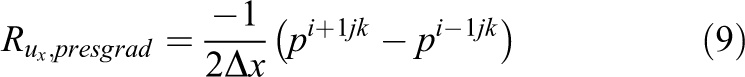
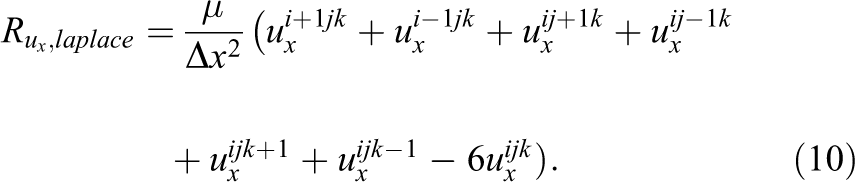
The spatial discretization is obtained by applying second order central differences on a globally uniform rectangular grid, which closely resembles the discretization possibilities of the LBM. As an example, residuals of the pressure gradient and the Laplace term are provided for the u_x velocity component:

$R_{u_x,presgrad}=\frac{-1}{2\Delta x}\left(p^{i+1jk}-p^{i-1jk}\right)$

9

$\begin{array}{c}{R}_{u_x,laplace}=\frac{\mu }{\Delta x^2}\left(u_x^{i+1jk}+u_x^{i-1jk}+u_x^{ij+1k}+u_x^{ij-1k}\right.\\ \left.+u_x^{ijk+1}+u_x^{ijk-1}-6u_x^{ijk}\right)\mathrm{.(10)}\end{array}$

10

All further terms, apart from the advection term, are discretized analogously. The advection term requires additional treatment to maintain the balance between the neighboring points. This is achieved by partially shifting the evaluation onto the edge in between the points. So far the resulting scheme has a compact stencil width of only two. However, the necessary stabilization, which is implemented as an adaptation of Jameson et al. (1981) using only the fourth-order artificial viscosity (AV), increases this width to four. It further introduces the parameter $c_{vel}$ that determines the influence of the stabilization and plays an important role in the later optimization.

The continuity equation is treated analogously to the momentum equations and is discretized with second order central differences and stabilized with fourth order AV. Here the additional parameter $c_{pres}$ is introduced.

The aforementioned methods are implemented in a highly tuned C/C++ code, for which a highly detailed description and analysis of the applied tuning techniques may be found in Wichmann et al. (2018). It utilizes an Array of Structure of Array (AoSoA) memory layout and incorporates spatial blocking (Datta et al. 2009) for maximal cache utilization. Additionally the actual simulation domain is padded by a layer of halo points for the application of boundary conditions which retains the ability to use a single long loop over the entire domain for evaluation. This reduces overhead for parallelization via OpenMP or offloading to GPUs (Löhner et al., 2014). The code is parallelized with OpenMP by loop tiling according to a lexicographic loop through the domain as detailed in Wichmann et al. (2018).

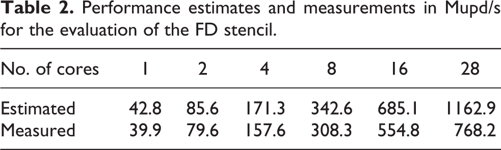
To demonstrate the competitiveness, some theoretical performance assessments of the plain stencil evaluation is provided. A total of 249.6 floating point instructions are required for the evaluation of the stencil in four points. This equates to 856.4 Mupd/s on the hardware used in this work. A tool assisted analysis that considers the parallel nature of the out-of-order execution of instructions showed that a reduced effort of 158.1 CPU cycles per four points can be assumed (Wichmann et al., 2018). This translates to 1842.2 Mupd/s.

If the performance is estimated in terms of memory bandwidth rather than arithmetic throughput, a different performance figure is obtained. A single point update requires loading 64B from and storing 32B to memory for all four components together when making full use of the spatial blocking. Measurements of the peak memory bandwidth on the employed hardware lead to 111.6 GB/s. The achievable bandwidth based throughput is therefore 1600 Mupd/s, which is lower than the arithmetic throughput and therefore more likely to be performance critical.

Applying the ECM model (Treibig and Hager, 2010), which additionally considers the arithmetic throughput and the interaction with the cache hierarchy, it is determined that the code is most likely limited by the arithmetic throughput for lower core counts. However, when using all available cores the arithmetic and bandwidth based limits approach each other, leading to an almost balanced CPU usage. The estimates and measurement are given in Table 2 and visualized in Figure 2. The expected initial linear scaling is almost matched by the measurements. At higher number of cores the measurements still reach 66.1% of the (bandwidth limited) estimate. Considering the complexity of the stencil, the spatial blocking adjusted to multiple cache levels and its interaction with the hardware, the number are reasonably close. For a detailed investigation refer to Wichmann et al. (2018).

Table 2.

Performance estimates and measurements in Mupd/s for the evaluation of the FD stencil.

No. of cores	1	2	4	8	16	28
Estimated	42.8	85.6	171.3	342.6	685.1	1162.9
Measured	39.9	79.6	157.6	308.3	554.8	768.2

In summary, the performance of the FDM is higher by a factor 3.5 than the LBM under ideal conditions. However, with smaller domain sizes the scaling is expected to degrade as the spatial blocking becomes less effective. The overall performance is therefore likely to be determined by algorithmic parameters, such as convergence behavior and accuracy of the method, which can influence the performance on orders of magnitude.

3. Comparison

The comparison is carried out on two steady-state and a transient test case. For the tests with steady flow, the main objective is the total time to solution at specific tolerances. To ensure that only the best set of parameters are compared, the following steps are applied to each method with every target tolerance separately.

First the simulation is set up with all parameters in a safe and stable range based on user experience. All parameters that do not alter the physics are then optimized automatically for the least amount of computational effort. When no further improvements can be achieved, the set of parameters is taken to stripped-down versions of the codes without any error evaluation. The full simulation duration is measured and the best out of 10 is considered to be the maximum performance. Carrying out the above steps for all cases enables the assessment of the methods’ performance in dependence of the target accuracy.

The transient test case is more closely oriented along common engineering practice. All the optimization steps in method-specific and code-specific parameters are performed on a precursor simulation with a steady flow. This is done under the same procedure as before, but only a single set of method-specific parameters is determined. This set of parameters is then transferred to the much more costly transient version. The runtime and accuracy of the full tests are then evaluated and compared.

The selection of the test cases is largely restricted by the capabilities and especially the union of capabilities of both codes. Since both methods operate on a globally uniform rectangular grid and we do not want to spoil the comparison by different ways of incorporating immersed boundaries, the domain is essentially restricted to a rectangular shape. Furthermore the supported types of boundary conditions are limited and especially corner cases for the LB method can cause difficulties. Also forcing is undesired, as it opens up to multiple choices on the incorporation into the LBM. Depending on the exact force and density properties of the flow, these can deeply influence the streaming and collision steps (Guo et al., 2002) and are not available in the highly tuned loop kernel. Therefore, the test cases of a duct flow compared to an analytical solution, a non-leaky lid driven cavity and the time-dependent flow around a cylinder with square cross section have been established as most suitable.

Once the optimal set of parameters is determined, the actual time measurements can be performed. This is carried out on the aforementioned 28 core dual socket Intel Xeon E5-2690 v4 with simultaneous multithreading (SMT) and Turbo Boost disabled. Also the CPU governor in the Linux kernel is in performance mode and higher C-states are disabled in order to minimize the noise in the measurements. Each code is stripped of unnecessary functionality, for example of the evaluation routines that are used for the optimization process. Since the required number of steps per tolerance is known from the optimization process it will be directly used for the measurement and no checks for convergence are performed. Both the GCC compiler (v6.3.0) and Intel compiler (v16.0.1) were applied to the codes. As expected for highly guided compilation the performance difference was below 1% in all cases with no clear advantage on either side. Due to easier accessibility GCC at high optimization settings (“-O3 -march=native”), taking full advantage of the four-fold vectorization and OpenMP parallelization was used. Compilation of the FDM kernel with additional “-ffast-math -funroll-loops -funsafe-math-optimizations -ftree-vectorize -fexcess-precision=fast” flags was found to generate the fastest and correct code. For further details on the configuration aspect refer to Wichmann et al. (2018).

3.1. Steady-state duct flow

3.1.1. Problem description

The first test case in this comparison is a steady-state duct flow. Due to its simplicity only a minimal set of features are required from both methods. Furthermore the analytical solution is known, eliminating uncertainty in the reference solution.

The duct, as depicted in Figure 3, has an aspect ratio of $L_x=15$ to $L_y=L_z=1$ . It is simulated at a Reynolds number of $Re=100$ , where $Re=\frac{U_{\text{max}}\cdot L_y}{\nu }$ . For the fully developed flow state the maximum velocity is at the center of the duct $U_{\text{max}}=U(x,\raisebox{1ex}{$L_y$}\!\left/ \!\raisebox{-1ex}{$2$}\right.,\raisebox{1ex}{$L_z$}\!\left/ \!\raisebox{-1ex}{$2$}\right.)$ , which can be inferred from the analytical solution. The artificial compressibility in both methods requires that the artificial speed of sound c_s is prescribed. It is determined by the Mach number $Ma=\frac{U_{\text{max}}}{c_s}$ , which is chosen as $0.1$ . This is in the incompressible regime, while offering fast convergence to a steady-state solution. By prescribing the maximum velocity as $U_{\text{max}}=1$ , the parameter of the speed of sound and the kinematic viscosity are obtained. An overview of all parameters for the duct flow is given in Table 3.

Figure 3.

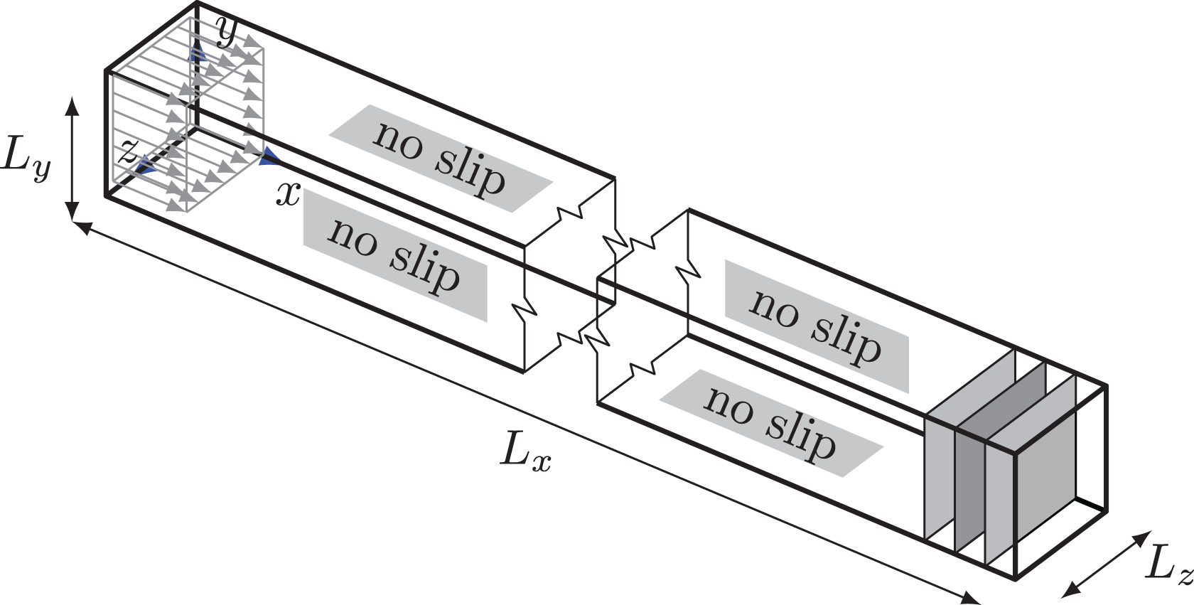
The duct flow setup with block inflow profile and error evaluation cross sections.

Table 3.

Problem specification of the duct flow.

Parameter	${\text{L}}_{\text{x}}$	${\text{L}}_{\text{y}}$	${\text{L}}_{\text{z}}$	${\text{U}}_{\text{max}}$	$\text{Re}$	$\text{Ma}$	$\rho$	$\nu$	$\raisebox{1ex}{$\text{d}p$}\!\left/ \!\raisebox{-1ex}{$\text{d}x$}\right.$	${\text{u}}_{\text{in,ideal}}$
Value	15	1	1	1	100	0.1	1	0.01	−0.13574	0.47704

A duct flow requires no-slip boundary conditions along the walls parallel to the flow direction ( $y=0$ , $y=L_y$ , $z=0$ , $z=L_z$ ). For the FDM the velocity at the wall is simply prescribed to zero and for the LBM the walls are implemented as midway bounce-back BCs. The inflow is realized as a block profile. The inflow velocity

$u_{in}(t)={\left(u_{in}\cdot \left(6{\widehat{t}}^5-15{\widehat{t}}^4+10{\widehat{t}}^3\right)\mathrm{,0,0}\right)}^T$

11

with $\widehat{t}=\text{min}\left(1,\frac{t}{t_{ramp}}\right)$ is applied to all inner nodes on the channel side $x\le 0$ . This greatly simplifies the boundary condition for the LB method, since no higher order moments arise, which would lead to transverse velocity components behind the inflow. At the outflow the pressure is prescribed to zero and there is no special treatment of the outgoing velocities.

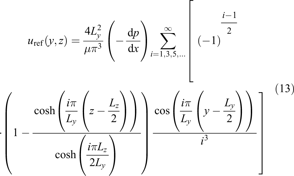
All error evaluations are carried out on the fully developed flow profile. For this a large part of the duct is dedicated to allow the block inflow to develop into the steady-state profile. In Figure 4 the error against the analytical solution on the cross section at the x-coordinate is shown. The error for the comparison is evaluated at $x=13$ , where the steady state is reached for all spatial resolutions relevant to this test. Slight differences in how the block profile of the inflow velocity is applied for each method are counteracted by choosing the inflow velocity $u_{in}$ in such a manner that the maximum velocity at $x=13$ is precisely one.

Figure 4.

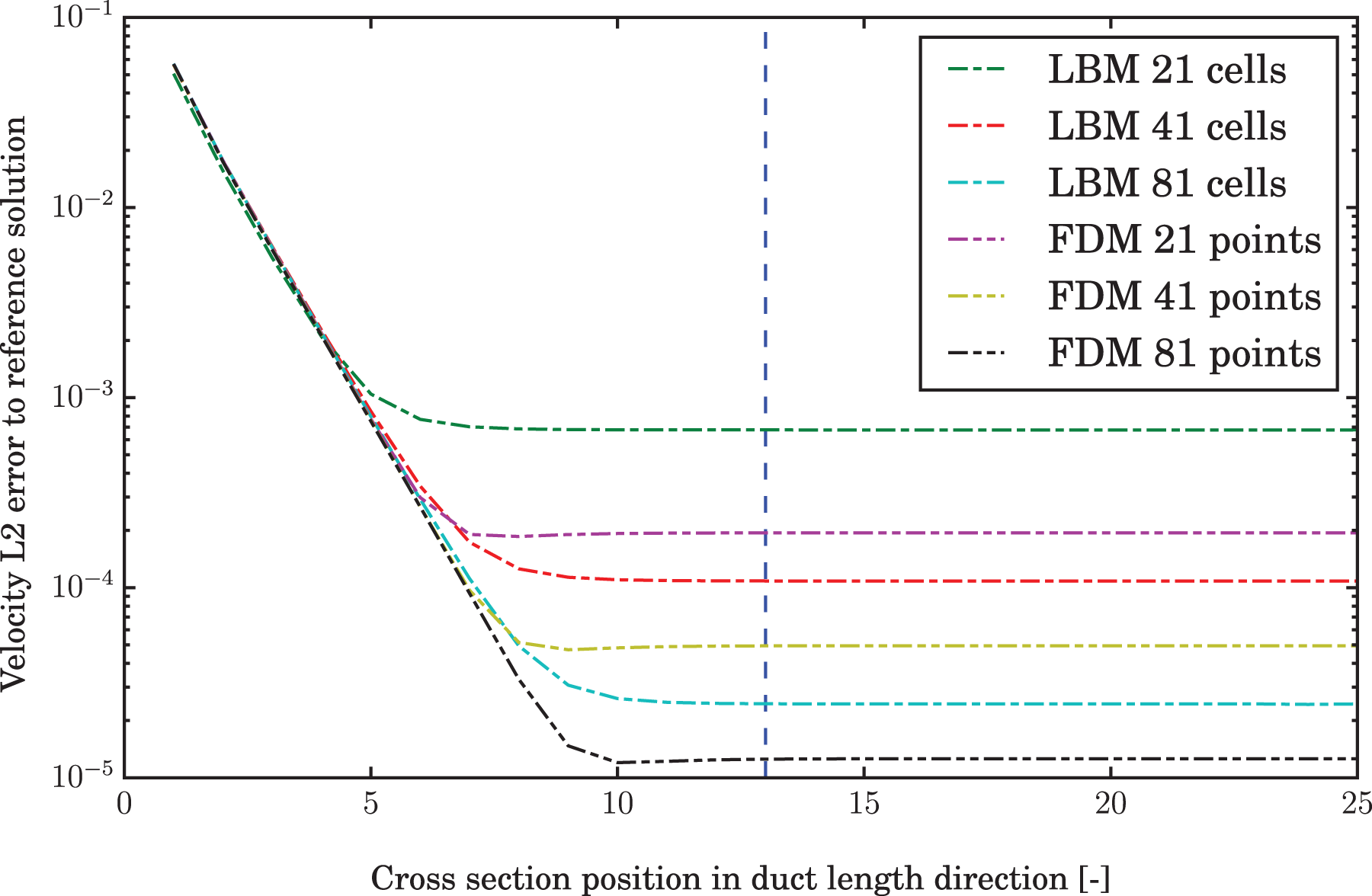
Development of error over channel length.

Three different error measures are used for the comparison. The first is the error in the fully developed velocity profile. It is determined by integrating the error in the L2-norm over the duct cross section

$e_u={\displaystyle \int }{‖u(13,y,z)-u_{ref}(13,y,z)‖}_2\text{d}y\text{d}z\mathrm{.}$

12

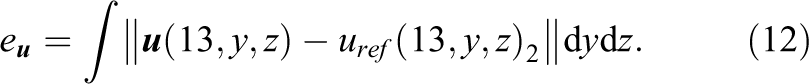
The necessary analytical solution $u_{\text{ref}}$ is obtained by numerically evaluating the infinite series

$\begin{array}{c}{u}_{\text{ref}}(y,z)=\frac{4L_y^2}{\mu {\pi }^3}\left(-\frac{\text{d}p}{\text{d}x}\right){\displaystyle \sum _{i=1,3,5,\mathrm{...}}^{\infty }}[(-1{)}^{\frac{i-1}{2}}\\ \left.\cdot \left(1-\frac{\text{cosh}\left(\frac{i\pi }{L_y}\left(z-\frac{L_z}{2}\right)\right)}{\text{cosh}\left(\frac{i\pi L_z}{2L_y}\right)}\right)\frac{\text{cos}\left(\frac{i\pi }{L_y}\left(y-\frac{L_y}{2}\right)\right)}{i^3}\right]\end{array}$

13

to 50 decimal places (White, 1991).

As the second quantity, the error in the pressure in the plane at $x=13$ is used. The pressure within this plane should be constant and by using the average pressure $〈p〉$ in said plane as the reference the error is independent of the exact working point of the outflow boundary condition. Integration of the error

$e_p={\displaystyle \int }\left|\frac{p(13,y,z)}{〈p(13,y,z)〉}-1\right|\text{d}y\text{d}z$

14

yields a scalar quantity which can readily be used for the assessment of the result quality.

The final error measure is the error in the pressure gradient $\raisebox{1ex}{$\text{d}p$}\!\left/ \!\raisebox{-1ex}{$\text{d}x$}\right.$ in the reference plane. The pressure gradient result is estimated by the difference in pressure between $x=12$ and $x=14$ and compared to the analytical pressure gradient readily available from the velocity solution mentioned above. The error

$e_{\frac{\text{d}p}{\text{d}x}}={\displaystyle \int }\left|\frac{p(14,y,z)-p(12,y,z)}{2}-\frac{\text{d}p}{\text{d}x}\right|\text{d}y\text{d}z$

15

is integrated in the same manner as before.

The total time to solution is determined by measuring the time until the simulations achieve a specified tolerance in the aforementioned L2 error. Artificial compressibility methods exhibit a distinct convergence behavior (see Figure 5) that is largely influenced by waves traveling through the domain. These waves decay slowly, but cause oscillations in the error. A tolerance is therefore considered reached when the error stays below the threshold permanently.

Figure 5.

Convergence of error in u_x at $x=13$ over time for FDM and LBM with 31 points/cells over the channel height.

The target tolerances are set to ${10}^{-3}$ , $\sqrt{10} \cdot {10}^{-4}$ and ${10}^{-4}$ , which are typical engineering choices. Any tighter tolerances are usually overshadowed by uncertainty in the choice of material parameters and geometry, outside academic examples (Lucor et al., 2003). Furthermore their costs are beyond the scope of an optimization process as applied here. A coarser choice of tolerances is excluded, since the simulations do not have to exhibit a proper convergence behavior, but can reach the target by coincidence.

Apart from the geometry, boundary conditions, error evaluation and tolerances, each method has some parameters that do not directly influence the physics. They do however influence the methods’ convergence behavior and evaluation cost. Since the best performance is of interest here, the simulations are tuned for minimal computational cost for every measurement. Simulation runs with different target tolerance can therefore have different optimal parameters.

The optimization is done by an automated process. As time measurements are subject to significant noise, the optimization is instead performed on an estimate of the computational cost, based on the number of time steps and cells/points. Another challenge is the abrupt change from faster convergence to divergence. Since we deal with an integer programming problem, gradient based optimization schemes are ruled out and instead a combination of bisection and hill climb is used.

For the finite difference approach, the most influential parameters are the number of discretization points and the CFL number. Another parameter is the ramping time $t_{ramp}$ (see (11)) determining the duration over which the inflow velocity is smoothly increased from zero. This ramp time determines how sharp the inflow velocity is applied and therefore the amplitude of the artificial wave that moves back and forth through the duct. Furthermore the stabilization parameters for the AV for the velocities $c_{vel}$ and the pressure $c_{pres}$ are optimized. Some exemplary results of the optimization are given in Figure 6(a).

Figure 6.

Simulation parameter optimization for the duct flow at $\sqrt{10} \cdot {10}^{-4}$ tolerance. Per pair of parameters the total number of point/site updates to solution is color-coded. The red line indicates non-converging settings. (a) FDM. (b) LBM.

The LB method requires fewer parameters to be optimized, since no stabilization is required for relaxation times within the stability range. The number of fluid cells, specified as the number of cells over the duct height, is again the most influential parameter. The second optimization parameter is the ramping time. Since the use of a cosine base ramping causes severe convergence problems if $t_{ramp}$ is not a multiple of the time step size, the polynomial in (11) was introduced.

Unlike the FDM, the equivalent to a CFL number for the LBM cannot be chosen explicitly. The LB velocities, cell spacing and time step sizes are bound to the used lattice. The factors for conversion between LB and physical dimensions are determined by the geometry for the cell size and the artificial Ma number for the velocity. The time step size is then readily available.

3.1.2. Results

The parameters resulting from the optimization process are given in Table 4. The FD method has five parameters that are optimized. Except for the number of discretization points and the velocity stabilization parameter, there is no smooth relation to the target error. This is due to the oscillating convergence behavior demonstrated in Figure 5, where a minute change can necessitate another cycle. The measurement of the number of time steps as integers leaves room for slight variations without resulting in an additional step. For this test case the velocity stabilization is, due to the nature of the flow, not required. The parameter has very little influence on the convergence speed, but leads to a slowdown if it is chosen too large. Regarding the LB method, a ramping of the inflow condition is not beneficial, instead it only delays convergence. It is apparent that the LB method requires more cells and more time steps than the FD method in order to meet the same tolerance. However, the difference in updates is relativized by the two Runge-Kutta stages the FDM employs and thus doing two updates per time step. Due to a mostly lower update rate (see introduction of both codes), the LB method is at a slight disadvantage for large domains or at strict tolerances. For coarse tolerances and the resulting smaller domains however the LBM's performance is on par, as the earlier bandwidth saturation is not as critical due to significant caching. The spatial blocking strategies of the FDM only show their full potential for large domains when all cache levels are used to reduce pressure on the memory interface.

Table 4.

Optimal performing parameters, errors, and timing results for the duct flow at multiple tolerances.

Tolerance	${\text{10}}^{-\text{3}}$	$\sqrt{\text{10}} \cdot {\text{10}}^{-\text{4}}$	${\text{10}}^{-\text{4}}$
FDM
Number of points over ${\text{L}}_{\text{y}}$	11	17	29
CFL number	0.866	0.85	0.806
Ramp time	3.125e−3	0.1	0.0
Stabilization pressure	0.11	0.11	9.195e−2
Stabilization velocity	0.165	0.15	8.018e−3
Number of time steps	3733	8855	16428
Pressure RMS error	1.594e−7	2.284e−5	1.675e−7
Pressure gradient L2 error	2.284e−4	4.541e−5	5.544e−6
LBM
Number of cells over ${\text{L}}_{\text{y}}$	21	27	49
Ramp steps	1	1	1
Number of time steps	10365	19765	31667
Pressure RMS error	2.954e−5	6.996e−6	2.039e−6
Pressure gradient L2 error	7.950e−6	1.612e−5	2.440e−6
Timings
FDM	1.936 s	10.269 s	53.188 s
LBM	2.132 s	33.361 s	288.079 s
Ratio	0.91	0.31	0.18

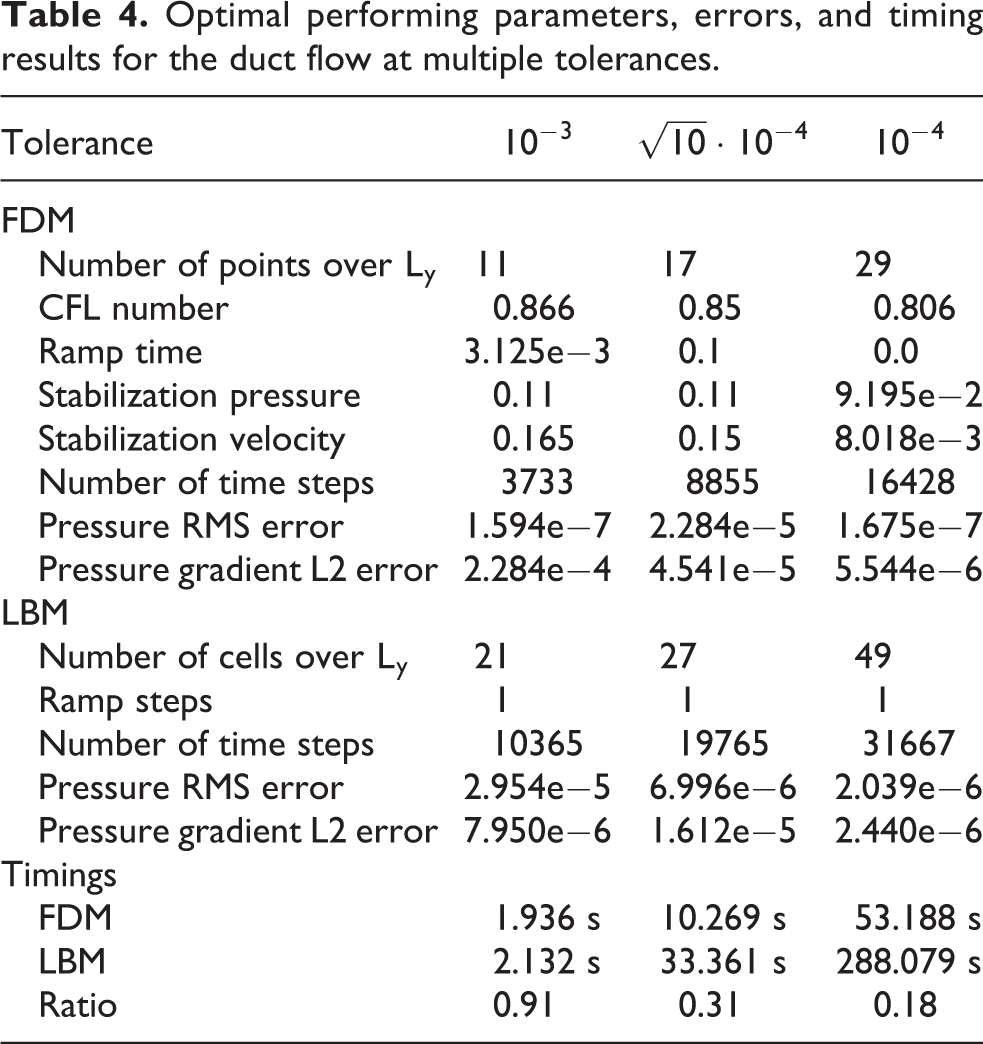
The measured elapsed times are provided in Table 4 and visualized in Figure 7. The FD method is significantly faster for the stricter tolerances with a factor of $5.4$ , which reduces to $1.1$ for less strict tolerances. The source of this difference in scaling behavior lies in the code performance and not the simulation method. The ratio of the number of cells over the channel height which are required for the LBM compared to the FDM reduces from $1.9$ to $1.7$ toward tighter tolerances and likewise the ratio of the number of time steps decreases from $2.8$ to $1.9$ . The code performance in terms of updates per second exhibits just the opposite behavior and dominates the overall timings. The reasons for the difference in code scaling are, as mentioned earlier, the spatial blocking in the FDM code which requires large block sizes to reach its full potential and the large load on the memory traffic of the LBM, which causes bandwidth saturation to set in for low core counts already and thus does not make full use of the available peak arithmetic throughput. A reduction of the LBM memory traffic by the indirect lookups only shifts the performance ratios, which makes the LBM faster at coarser tolerances, but does not alter the overall behavior.

Figure 7.

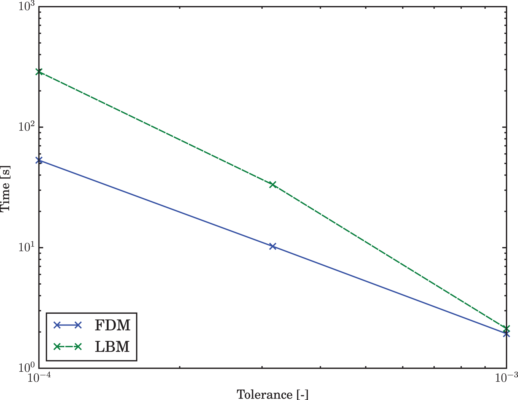
Total time to solution over the tolerance for the duct flow.

3.2. Lid driven cavity

3.2.1. Problem description

The second test case is a flow in a lid driven cavity. It constitutes a significantly more complex flow pattern and has seen a lot of studies over the years as the one by Shankar and Deshpande (2000). As opposed to the duct flow, the convection term plays a crucial role in the steady-state solution.

In literature most commonly the leaky lid driven cavity is studied. However, the in- and outflow gaps are not straight forward to set up in the lattice Boltzmann context. The complex interactions between the many density distributions on the interface of adjacent BC types require separate handling with complex terms in order to maintain good convergence rates. This contradicts the performance aspect. Additionally it is difficult to keep the boundary condition at the midway point between cells in this corner case, causing problems in maintaining the gap size and making it difficult to ensure equal behavior in these regions between the LBM and the FDM. An alternative would be using the section between the edge points and their next neighbors as the gap, but this leads to singularities in the corners, just as it does for the non-leaky lid driven cavity. This is of course not suitable for a comparison which is also based on convergence. However, the non-leaky variant can be modified to suppress the singular behavior by prescribing a velocity profile on the lid, which naturally tends toward a zero velocity at the edges.

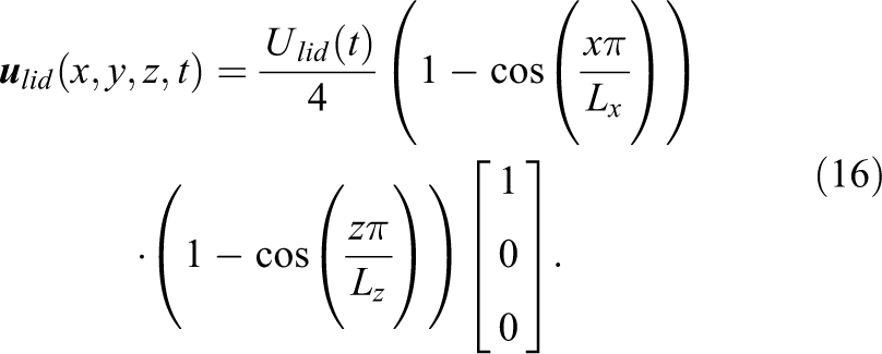
The problem to be solved is illustrated in Figure 8. It shows the three-dimensional non-leaky steady-state lid driven cavity with an aspect ratio of 1:1:3. The lid (min y) is driven by a Dirichlet boundary condition prescribing the following profile

$\begin{array}{c}{u}_{lid}(x,y,z,t)=\frac{U_{lid}(t)}{4}\left(1-\text{cos}\left(\frac{x\pi }{L_x}\right)\right)\\ \cdot \left(1-\text{cos}\left(\frac{z\pi }{L_z}\right)\right)\left[\begin{array}{c}1\\ 0\\ 0\end{array}\right].\end{array}$

16

Figure 8.

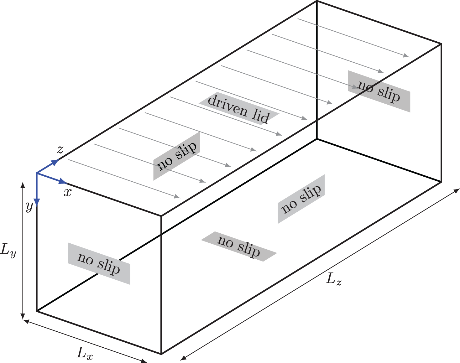
The 3D non-leaky lid driven cavity.

In the LB context non-constant BCs, such as the one above, require advanced schemes. Straight forward application of a bounce-back condition can lead to the introduction of spurious velocities through higher order moments, while more complex approaches increase the computational effort. A balance between those two goals is the use of a correction term, such as proposed by Hecht and Harting (2010), which is used here.

The cavity is simulated at a Reynolds number of $Re=100$ , where the Reynolds number is defined via the maximum lid velocity and the cavity length in flow direction $Re=\frac{U_{lid}{L}_x}{\nu }$ . As before the artificial compressibility nature of the methods gives rise to an artificial Mach number, which is set to $Ma=0.1$ . All simulations are started from a zero initial field and the lid velocities are ramped up to the final value using the polynomial from (11). A summary of the parameters for the LDC is given in Table 5.

Table 5.

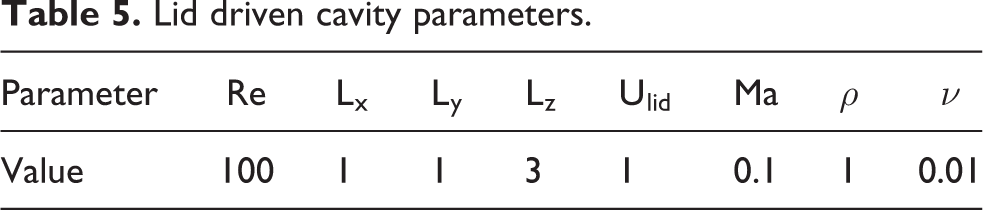
Lid driven cavity parameters.

Parameter	Re	${\text{L}}_{\text{x}}$	${\text{L}}_{\text{y}}$	${\text{L}}_{\text{z}}$	${\text{U}}_{\text{lid}}$	Ma	$\rho$	$\nu$
Value	100	1	1	3	1	0.1	1	0.01

For the error evaluation, no analytical solution is available. Instead reference solutions are computed by performing simulations at a much finer spatial resolutions with each method, as well as an additional finite element code. The finite element simulation is performed using an implicit steady-state simulation with hexahedral inf-sup stable finite elements of velocity degree 4 and pressure degree 3 and is designed to solve the incompressible Navier–Stokes equation in the most direct fashion. The FEM code is openly available (Kronbichler et al., 2018) ¹ .

For each method two separate convergence results are shown Figure 9. The solid lines are the convergence behaviors that the methods exhibit when each method is compared against its own results on the finest resolution. The dashed lines correspond to the results with the finite element solution as the reference instead.

Figure 9.

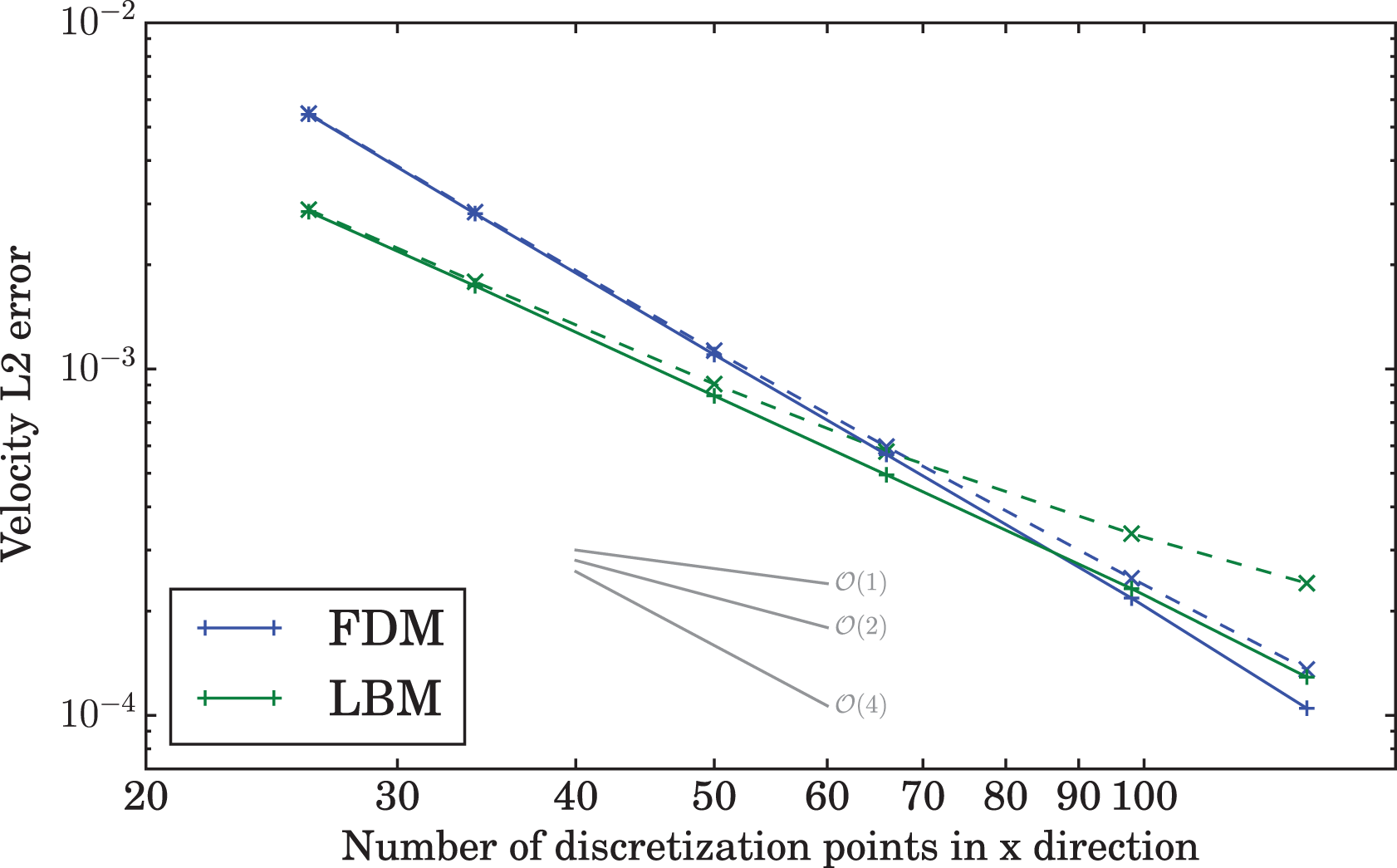
Convergence rates of LBM and FDM codes for the LDC problem. The dashed lines use the FEM solution as the reference.

In the case that each method uses its own reference result, the convergence matches the expected behavior. The finite element simulation converges with fourth order, while the finite difference approach converges at second order. For the lattice Boltzmann method there is no definite expected convergence rate for this case (see LBM description), but it can be up to second order. Hence the measured order of $1.89$ is a good match.

When the error of all methods is evaluated relative to the finite element reference results, the convergence orders decrease slightly. This effect is more pronounced at finer discretizations, which is partially due to well-known effect of increased convergence rates when comparing to a result with the same dominating error at a marginally higher resolution. Furthermore, it indicates that the methods converge toward slightly different solutions.

For the above case the compressibility exhibited by the LBM and FDM can be ruled out as a cause, since both methods only exhibit compressibility while approaching the steady state. Once this state is established, as in this convergence study, the compressibility effect vanishes completely.

For the actual measurements however, the compressibility when the coarse tolerances of ${10}^{-3}$ , $\sqrt{10}\cdot {10}^{-4}$ and ${10}^{-4}$ are reached, is still significant. Since this is a characteristic of the methods it is included in the comparison. In fact, it is one of the strongest influences on the performance results and overshadows any errors introduced by differences in reference results. However, since a definite reference cannot be established and to ensure that the methods are treated in fair manner each method will be using its own reference.

The error evaluation for the LDC is not as straight forward as for the duct flow, as the simulation results are discretized differently than the reference results. In order to minimize the impact of this discrepancy the velocity error is determined by point-wise integration of the coarser domain and interpolation of the finer domain for the difference evaluation. Three-dimensional piece-wise fourth degree Lagrangian polynomials are used to ensure high quality interpolation. Tests showed that the influence on the error near the target tolerances is $<0.001\%$ and thus negligible. Note that the error evaluation for the LBM is carried out in the physical domain, i.e. all results in LB units are scaled using the discrete variables ${\delta }_x$ and ${\delta }_t$ .

Analogously to the duct flow, the lid driven cavity simulations are optimized for minimal computational cost. The target tolerances for the velocity error are ${10}^{-3}$ , $\sqrt{10} \cdot {10}^{-4}$ and ${10}^{-4}$ . For each tolerance and each method the same set of parameters as for the duct flow is optimized. As an example the number of discretization points in x-direction over the CFL number for the FDM is given in Figure 10(a) and the number of lattice cells in x-direction over the number of ramping steps for the LBM is shown in Figure 10(b).

Figure 10.

A selection of the simulation parameter optimization for the non-leaky LDC at ${10}^{-3}$ tolerance. Per pair of parameters the total number of point/site updates to solution is color-coded. The red line indicates non-converging settings. (a) FDM. (b) LBM.

3.2.2. Results

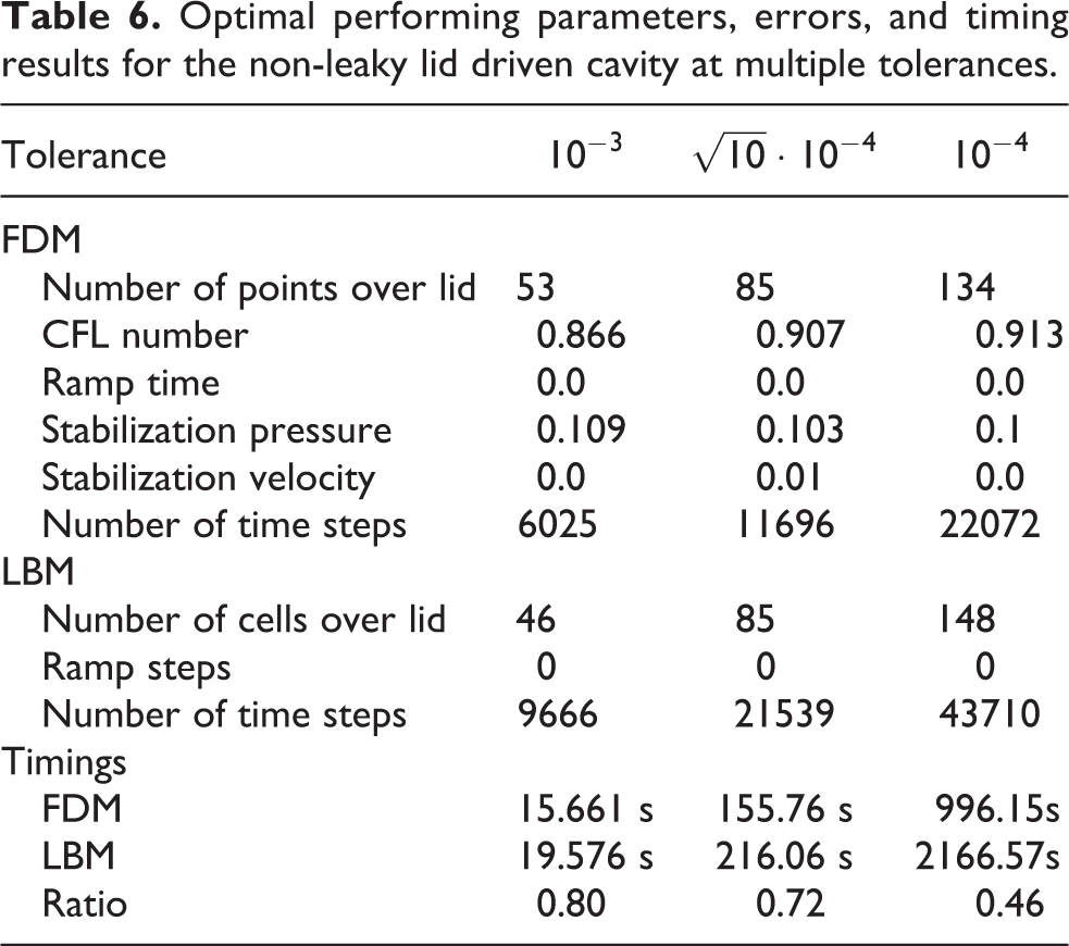
The results of the optimization process are given in Table 6. Similar to the duct flow there is no direct and smooth relationship between the tolerance and the set of optimal parameters. The required spatial resolution toward stricter tolerances grows more quickly for the LBM than the FD method. The same holds for the number of time steps. This causes the performance gap in the actual time to solution, shown in Table 6 and Figure 11, to increase for stricter tolerances. As for the duct flow this gives a clear performance advantage for the FDM, especially for higher quality results. Also a subtraction of indirect memory accesses for the LBM merely shifts the timings slightly, such that the break even point would occur at a slightly stricter tolerance than ${\text{10}}^{-\text{4}}$ .

Table 6.

Optimal performing parameters, errors, and timing results for the non-leaky lid driven cavity at multiple tolerances.

Tolerance	${\text{10}}^{-\text{3}}$	$\sqrt{\text{10}} \cdot {\text{10}}^{-\text{4}}$	${\text{10}}^{-\text{4}}$
FDM
Number of points over lid	53	85	134
CFL number	0.866	0.907	0.913
Ramp time	0.0	0.0	0.0
Stabilization pressure	0.109	0.103	0.1
Stabilization velocity	0.0	0.01	0.0
Number of time steps	6025	11696	22072
LBM
Number of cells over lid	46	85	148
Ramp steps	0	0	0
Number of time steps	9666	21539	43710
Timings
FDM	15.661 s	155.76 s	996.15s
LBM	19.576 s	216.06 s	2166.57s
Ratio	0.80	0.72	0.46

Figure 11.

Total time to solution for the non-leaky LDC.

3.3. Transient flow around a cylinder with square cross section

3.3.1. Problem description

Continuing toward typical applications of CFD in engineering, the following test case offers an additional level of complexity at the cost of more uncertainty in the reference result. As depicted in Figure 12, the setup is a duct flow with a slightly off-centered obstacle in the form of a rectangular cuboid. This configuration is also referred to as a flow around a cylinder with square cross section. Especially through the off-centeredness complex flow phenomena can be observed, while the overall geometry is very simple. This makes it a popular test case for comparisons that has been studied in many variations in Schäfer et al. (1996), Sohankar et al. (1999), Breuer et al. (2000), Saha et al. (2003), Sen et al. (2011) and Klein et al. (2015), including experimental work by Okajima (1982) and Knisely (1990).

Figure 12.

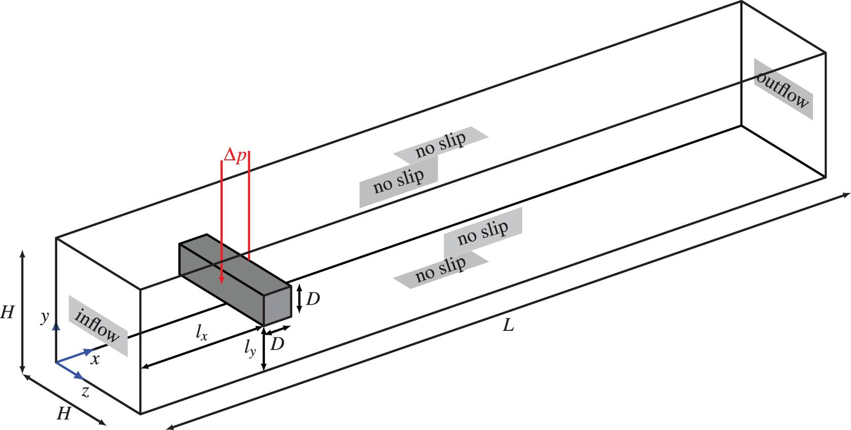
Setup of the flow around a square cylinder.

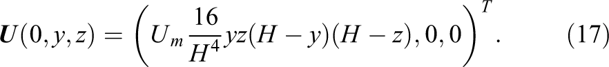
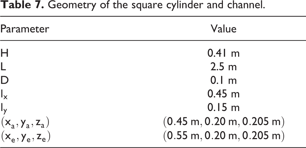
The geometrical simplicity has some major advantages, as it reduces the need for sophisticated boundary conditions since all boundaries are orthogonal to the coordinate directions and thus reduces the impact of the choice of boundary condition method. The exact set up is specified in Table 7 and is based on the configurations used in Schäfer et al. (1996) for comparison purposes. The inflow at $x=0$ is prescribed as a parabolic velocity profile according to

$U(0,y,z)={\left(U_m\frac{16}{H^4}yz\left(H-y\right)\left(H-z\right)\mathrm{,0,0}\right)}^T\mathrm{.}$

17

Table 7.

Geometry of the square cylinder and channel.

Parameter	Value
H	0.41 m
L	2.5 m
D	0.1 m
${\text{l}}_{\text{x}}$	0.45 m
${\text{l}}_{\text{y}}$	0.15 m
${\text{(x}}_{\text{a}}{\text{,y}}_{\text{a}}{\text{,z}}_{\text{a}}\text{)}$	$\text{(0.45}\hspace{0.17em}\text{m,0.20}\hspace{0.17em}\text{m,0.205}\hspace{0.17em}\text{m)}$
${\text{(x}}_{\text{e}}{\text{,y}}_{\text{e}}{\text{,z}}_{\text{e}}\text{)}$	$\text{(0.55}\hspace{0.17em}\text{m,0.20}\hspace{0.17em}\text{m,0.205}\hspace{0.17em}\text{m)}$

The maximum inflow velocity U_m is prescribed at several different values, which gives direct control over the Reynolds number and hence the flow patterns.

The resulting flow phenomena are one way of judging the quality of the solution. The vortex shedding is very sensitive and the shedding frequency is one of the indicators used in the following. Further scalar quantities typical in engineering are the lift and drag forces on the cylinder. Due to the slight asymmetry in the cylinder positioning, these forces also arise in a steady flow. This is exploited in the following by setting up and optimizing most parameters with the help of much faster steady simulations and subsequent transfer to a transient case. The lift F_L and drag F_D are compared in their non-dimensional form

$c_L=\frac{2F_L}{\rho {\overline{U}}^{2}DH},c_D=\frac{2F_D}{\rho {\overline{U}}^{2}DH},$

18

where $\overline{U}=\frac{4}{9}{U}_m$ is the characteristic velocity. The techniques for obtaining the resultant force on the cylinder differ between FDM and LBM. For the FDM stress integration is carried out on all four sides with the readily available velocities and pressures. The derivatives are approximated using higher order difference on the existing grid. Separation into duct length-wise and orthogonal direction yield

$F_D={\displaystyle {\int }_S}\left(\rho \nu \frac{\partial u_t}{\partial n}{n}_y-p{n}_x\right)dS,$

19

$F_L={\displaystyle {\int }_S}\left(\rho \nu \frac{\partial u_t}{\partial n}{n}_x-p{n}_y\right)dS,$

20

respectively. The same technique can also be used for the lift and drag evaluation in LBM simulations by applying the stress integration to the recovered velocities and pressure. However, an easier and more accurate approach is the use of the momentum exchange method by Yu et al. (2003). It capitalizes on the fact that the transported density distribution carry a linear momentum that is altered by the bounce-back on the obstacle boundary. By directly summarizing the momentum of affected distributions $f_{i_b}$ in the direction leaving the obstacle $i_b\left(x_b\right)$ of cells that form the boundary x _b the resultant force is obtained as

$F={\displaystyle \sum _{x_b}}{\displaystyle \sum _{i_b\left(x_b\right)}}2f_{i_b}\left(x_b,t\right)c_{i_b}\frac{{\delta }_x^4}{{\delta }_t^2}\mathrm{.}$

21

The list of measures is further supplemented by the pressure delta

$\Delta P=P(x_a,y_a,z_a)-P(x_e,y_e,z_e)$

22

across the centers of the front and back face of the cylinder.

3.3.2. Laminar precursor simulation

As noted above the test case of the flow past a cylinder with square cross section can easily be simulated in steady or transient configurations. This is used to carry out the parameter optimization on the considerably cheaper steady problem. The simulation specification for these precursors are provided in Table 8. The optimized code parameters, which are obtained through optimization of the steady case are identical with optimal parameters of the transient case. These parameters are fully decoupled from the problem that is being solved, apart from the grid/lattice layout. The same spatial resolutions are utilized for the steady and the transient versions.

Table 8.

Parameters specific to the laminar flow around a cylinder with square cross section.

Parameter	Value
Ma	0.1
Re	20
$\rho$	$\text{1} \hspace{0.17em}\text{kg} {\text{m}}^{-\text{3}}$
${\text{U}}_{\text{m}}$	$\text{0.45} \text{m} {\text{s}}^{-\text{1}}$
$\nu$	$\text{0.001} {\text{m}}^{\text{2}} {\text{s}}^{-\text{1}}$

Other than the code parameters the optimized simulation parameters, such as stabilization factors and spatial resolution, are not independent of the problem setup. However, a complete search for the ideal set of parameters as carried out for the duct flow and the lid driven cavity is much too costly to be performed with the full transient flow. The test case of the steady flow is not only useful as the precursor to the transient case. Even by itself it is an interesting test case for which reference results are available through Schäfer et al. (1996).

The setup of the flow past a cylinder with square cross section for the FDM is fairly straight forward since the geometry allows a body-fitted grid to be used, even with globally uniform grid. The only limitation is that a length of 0.01 m must be evenly divisible by the grid spacing. By omitting the number of ramp-up steps, which cannot be applied to the transient case anyway, the search space for optimal parameters is significantly reduced. The remaining options of CFL number, velocity and pressure stabilization factor are optimized one by one iteratively. There are three measures that are used to judge the solution and which potentially require different configuration for optimal performance. As the goal is the shortest overall simulation runtime, the parameters are tuned for all three measures simultaneously by utilizing the maximum of the time steps required to reach each of the targets. The resulting ideal simulation parameter set is listed in Table 9. As noted previously, the ideal code parameters only depend on the domain dimensions and hardware. Through brute force search for all spatial resolutions the fastest code set ups were tabulated and reused for all further simulations.

Table 9.

The optimized simulation parameters for the flow around a cylinder with square cross section using the FDM.

CFL number	${\text{c}}_{\text{velo}}$	${\text{c}}_{\text{pres}}$
0.116	0.54	0.74

The parameter optimization is even easier for the LBM, as there are no simulation parameters free for tuning. For the code parameters the same as for the FDM holds true and identical brute force strategy for optimization is used.

3.3.3. Laminar flow

The results with respect to the solution quality and the simulation runtime of the steady-state problem are presented in the following. The solution of either method roughly matches the results published in Schäfer et al. (1996). The suggestions of the valid ranges published therein are provided alongside the FDM and LBM results in Figure 13. It should be noted that the reference was generated using very few degrees of freedom, compared to today’s standards, and can only be taken as a rough guidance. It is therefore not critical that the LBM results for the drag converge toward a value outside the published range, as shown in Figure 13(b), and which actually matches the behavior of a LBM simulation provided in Schäfer et al. (1996).

Figure 13.

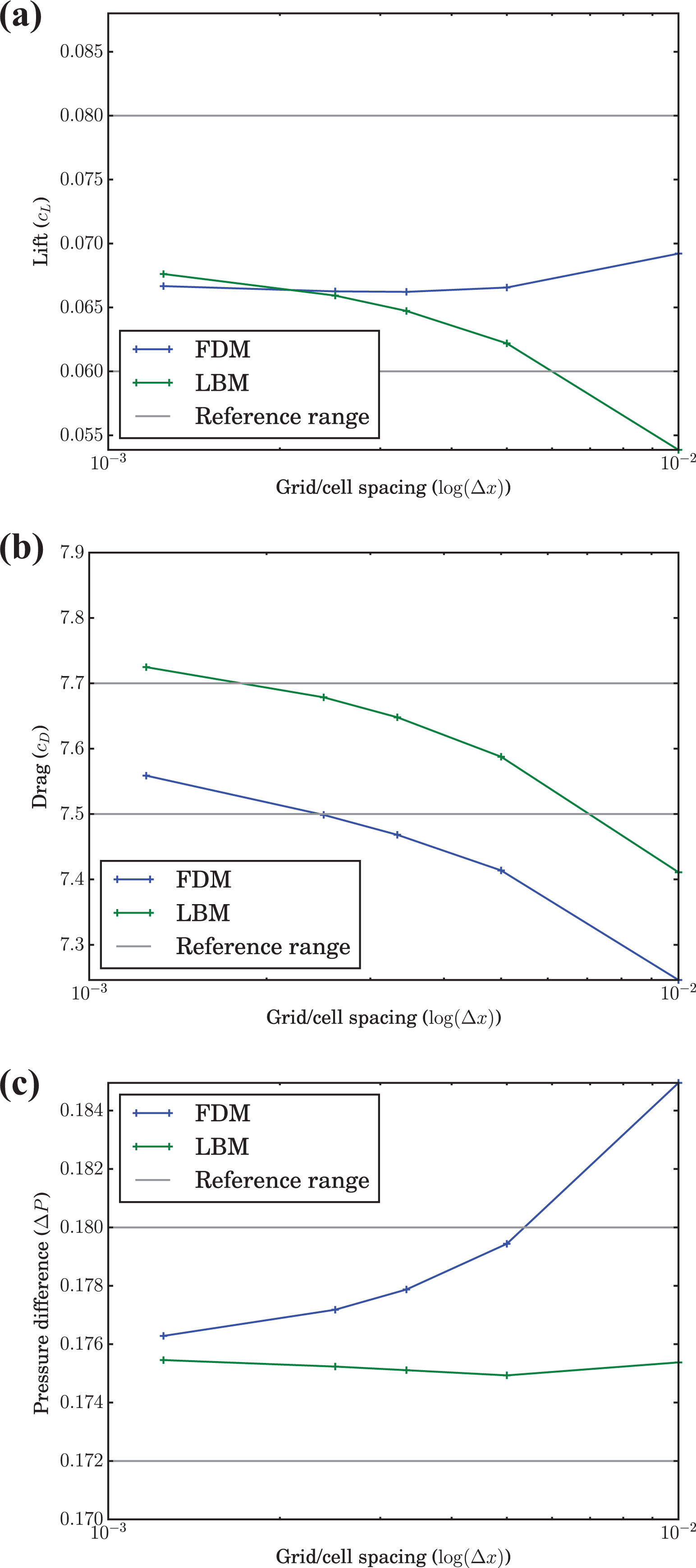
Lift, drag, and pressure difference results for the steady flow past a cylinder with square cross section simulated with the FDM and LBM. The reference ranges are taken from Schäfer et al. (1996). (a) Lift. (b) Drag. (c) Pressure difference.

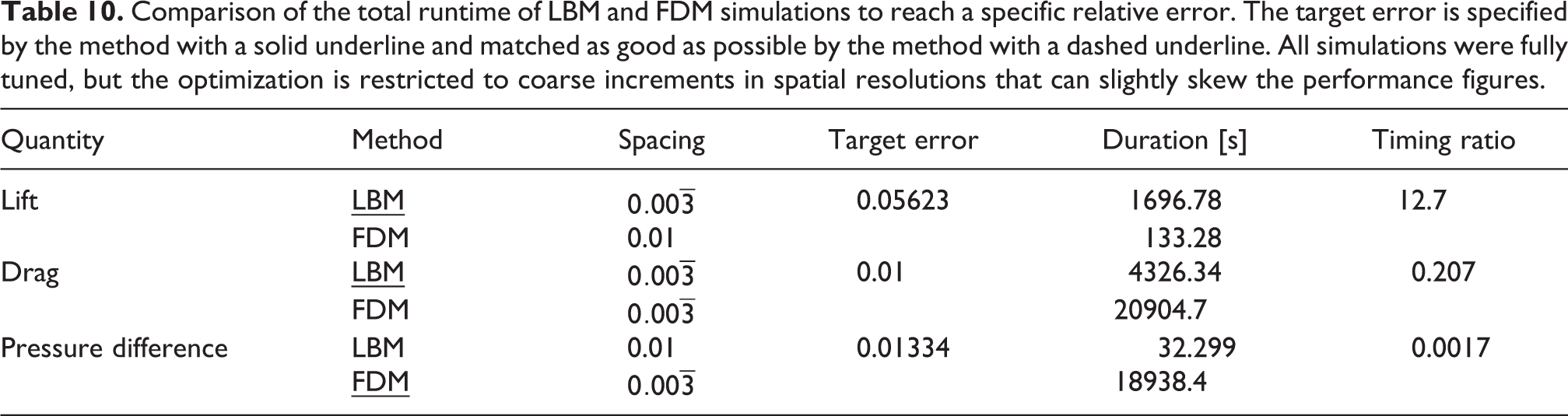
A fair performance comparison following the same scheme as with the previous test cases is impractical for the flow past a cylinder. The coarse steps in which the spatial resolution can be increased and the large impact of the resolution on the overall runtime make the approach of tuning for a specific error unsuitable. The numbers provided in Table 10 can therefore only be taken as estimates. In fact they only show the upper limit of the performance ratio. This is due to the target error being set by one method (solid underline in Table 10) and which is then matched as good as possible by the other method (dashed underline) at a likely non-ideal resolution. A more thorough performance investigation is carried out for the transient test case. The steady flow version is primarily used for the optimization of code and simulation parameters.

Table 10.

Comparison of the total runtime of LBM and FDM simulations to reach a specific relative error. The target error is specified by the method with a solid underline and matched as good as possible by the method with a dashed underline. All simulations were fully tuned, but the optimization is restricted to coarse increments in spatial resolutions that can slightly skew the performance figures.

Quantity	Method	Spacing	Target error	Duration [s]	Timing ratio
Lift	LBM	$\text{0.00}\overline{\text{3}}$	0.05623	1696.78	12.7
	FDM	0.01		133.28
Drag	LBM	$\text{0.00}\overline{\text{3}}$	0.01	4326.34	0.207
	FDM	$\text{0.00}\overline{\text{3}}$		20904.7
Pressure difference	LBM	0.01	0.01334	32.299	0.0017
	FDM	$\text{0.00}\overline{\text{3}}$		18938.4

3.3.4. Transient flow

The transient version is identical in set up to the steady-state version presented above, with some alterations to the inflow parameters listed in Table 11. Furthermore the inflow velocity profile given in equation (17) is multiplied by the time-dependent component $\text{sin}\left(\pi \frac{t}{8}\right)$ over the time span from 0 to 8 seconds. Even though the weakly compressible methods used here are not time-accurate, they can still yield good results if the problem is not highly transient. There are remedies for the FDM in the form of dual-time stepping schemes (Merkle, 1987) for example, however, since nothing comparable is known for the LBM it is not considered further for the sake of comparability. As the reference result to judge the solution quality against, a very high resolution result was produced with the high-order implicit FEM code from Kronbichler et al. (2018).

Table 11.

Parameters specific to the transient flow around a cylinder with square cross section.

Parameter	Re	$\rho$	${\text{U}}_{\text{m}}$	$\nu$
Value	100	$\text{1}\hspace{0.17em} \text{kg} {\text{m}}^{-\text{3}}$	$\text{2.25}\hspace{0.17em} \text{m} {\text{s}}^{-\text{1}}$	$\text{0.001}\hspace{0.17em} {\text{m}}^{\text{2}} {\text{s}}^{-\text{1}}$

The timed simulations with the FDM and LBM are carried out using the optimized parameters from the steady flow. While these may not be fully optimal, there is some noise in determining these anyways and the impact of small imperfections near the optimal configuration is very small.

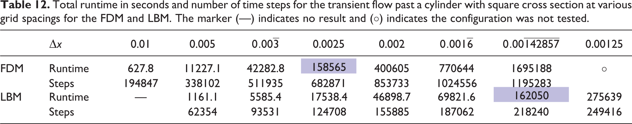
In Figure 14 the lift and drag coefficient over the time span of 8 s is provided. Figure 14(a) and (b) show the influence of different resolutions, simulated with the FDM, while the Figure 14(c) and (d) show the same for the LBM. The dashed line is the reference result that is taken from the highest resolution result of the FEM simulations. Several effects are immediately apparent from these results. For one, all curves are superposed with some higher frequency oscillation typical for weakly compressible methods. This effect is particularly pronounced at the start of each run, due to the shock induced by the jump start that slowly fades away. Note especially the spikes in drag, which are almost identical between the FDM and LBM and show how similar both methods are. The other apparent effect is a much slower convergence of the FDM with regard to spatial resolution, compared to the LBM. This is more pronounced for the lift coefficient than the drag. However, it can also be seen that the LBM converges toward a slightly different result than the FEM reference and the FDM. It is very difficult to exactly quantify the deviations from the desired reference. Especially the superposition of the overall error with the oscillations due to the weakly compressible nature give room to differently weigh these errors. As the importance of the errors is highly dependent on the purpose of the simulation, it impossible to judge the result quality as a single scalar without any bias. To allow for a direct comparison nonetheless a different and partially qualitative approach is employed. Rather than tuning for a specific error, a sequence of simulations at different resolutions is measured and two similarly timed configurations are compared for their error. A summary of the runtimes for all configurations is provided in Table 12. The highlighted runs are within 2.2% of each other in terms of total runtime and are hence ideal candidates for a closer look. Figure 15 gives a direct comparison of the FDM result with a spacing of $0.0025$ and the LBM at a spacing of $0.00143$ . Even without any specific quantification the vastly better results of the LBM for the lift can be observed. For example it takes less than half the cell spacing of the FDM and less than a 300th of the total runtime to produce similar results. However, there is some limitation to this performance advantage. The LBM solution overshoots the reference results and converges to different solutions. Naturally the achievable error is limited by this effect. The FDM on the other hand may converge more slowly and at higher computational cost, but it shows no sign of converging to a different solution and thus becomes the faster and eventually the only choice for stricter tolerances.

Figure 14.

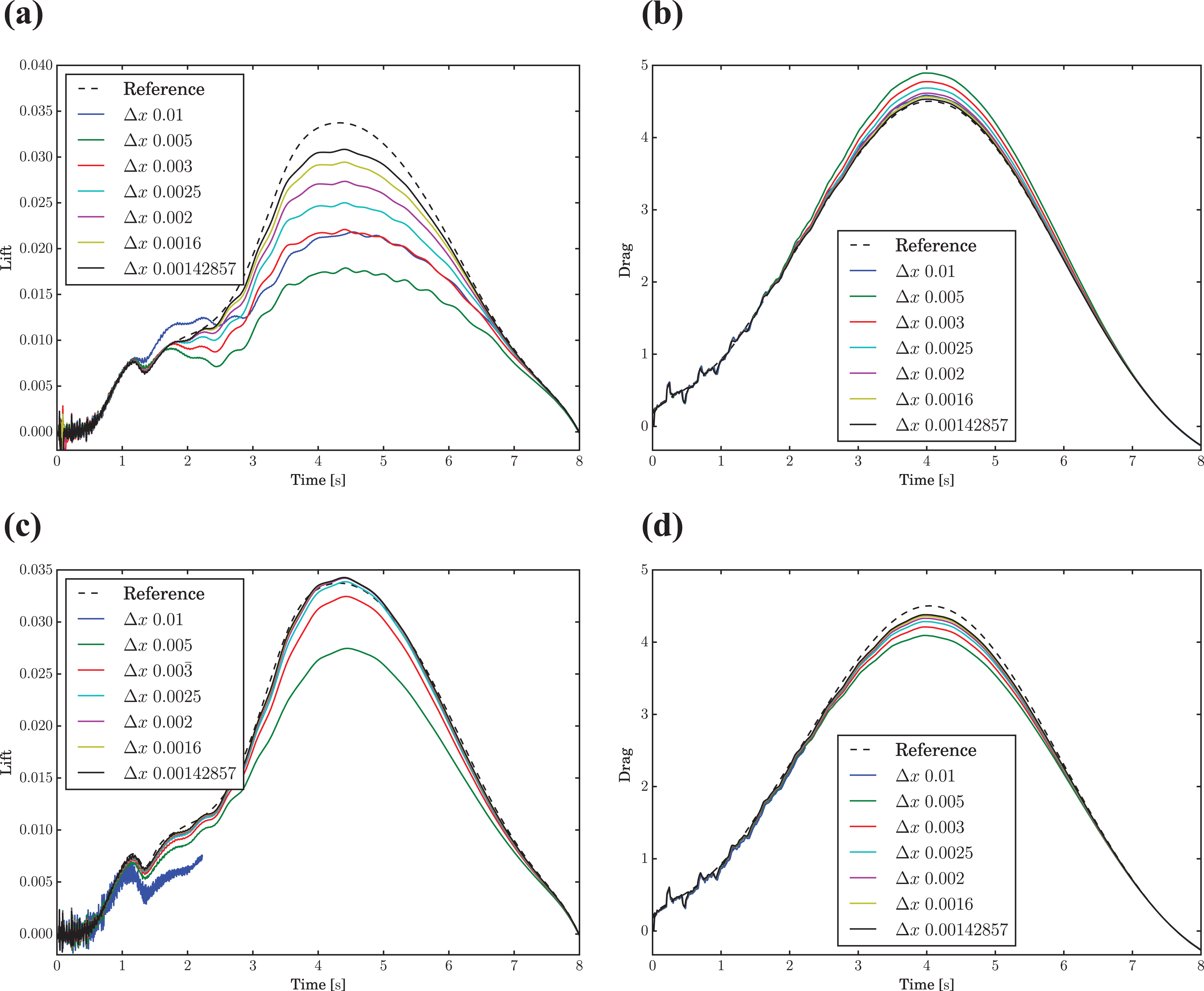
Lift and drag over the time span of 8 s at different grid/lattice spacings for $\text{Ma}=0.1$ .

Table 12.

Total runtime in seconds and number of time steps for the transient flow past a cylinder with square cross section at various grid spacings for the FDM and LBM. The marker (—) indicates no result and ( $\circ$ ) indicates the configuration was not tested.

	$\Delta x$	0.01	0.005	$\text{0.00}\overline{\text{3}}$	0.0025	0.002	$\text{0.001}\overline{\text{6}}$	$\text{0.00}\overline{\text{142857}}$	0.00125
FDM	Runtime	627.8	11227.1	42282.8	158565	400605	770644	1695188	$\circ$
	Steps	194847	338102	511935	682871	853733	1024556	1195283
LBM	Runtime	—	1161.1	5585.4	17538.4	46898.7	69821.6	162050	275639
	Steps		62354	93531	124708	155885	187062	218240	249416

Figure 15.

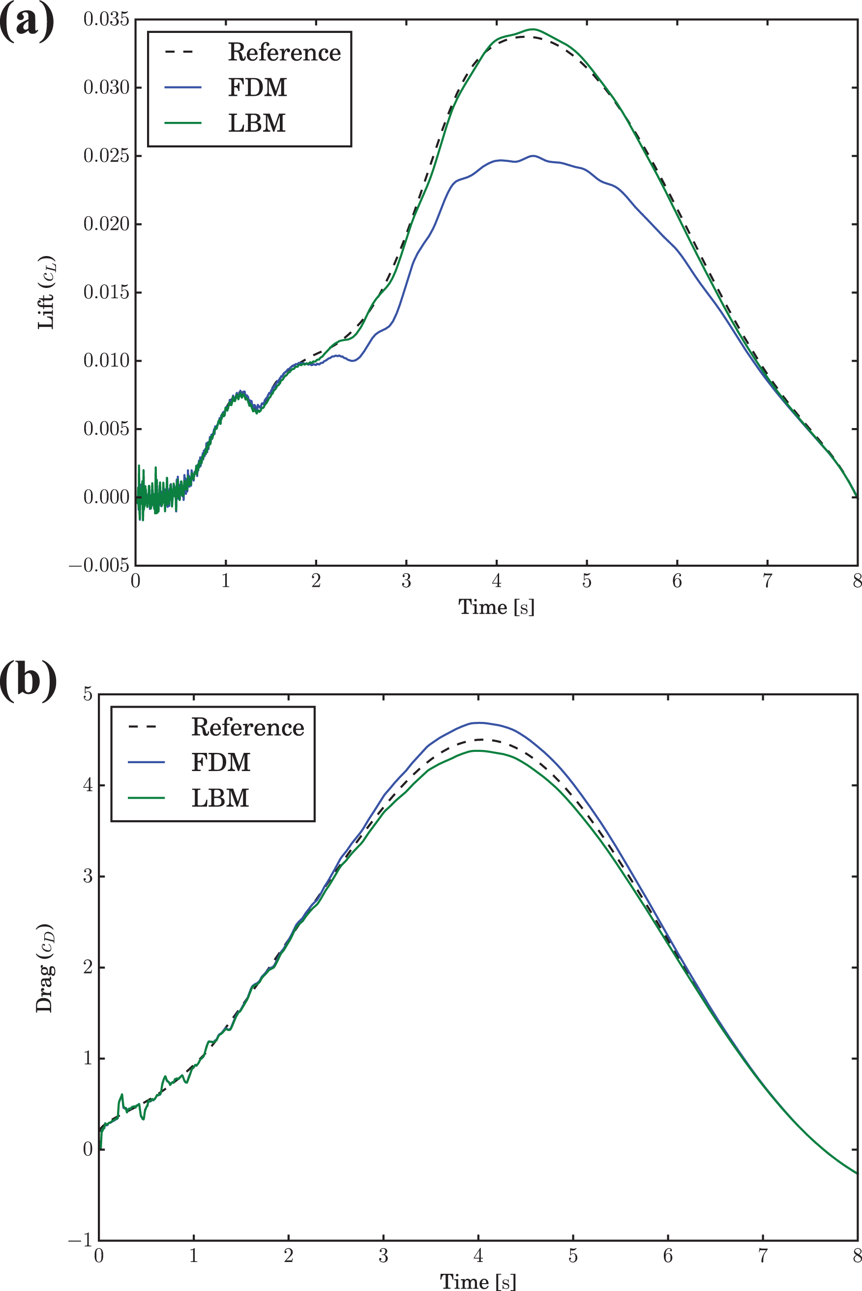
Lift and drag for FDM and LBM simulations at a comparable total run time. (a) Lift. (b) Drag.

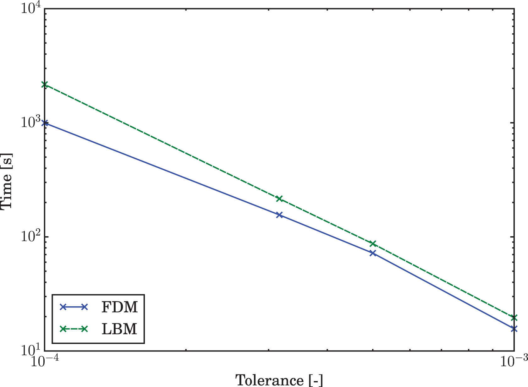
This difference is less pronounced for the drag coefficient. Due to the almost identical behavior of the higher frequency errors, the overall error can be reliably determined by the maximum of the drag, for example. This leads to a relative error of 2.7% for the LBM and 4.1% for the FDM. In the following these qualitative results are supplemented with quantification of a single carefully selected measure. This quantification is achieved by interpolating the required resolution for a particular error and calculating the total runtime for this theoretical grid. Figure 16(a) shows the error in the maximum drag for different spatial resolutions, compared the reference result. Since the smallest error that is reached by the LBM is larger than for the FDM, its error is matched by interpolating the FDM error and determining the required resolution. The resulting grid spacing is then used to determine the simulation duration, as shown in Figure 16(b). To obtain a better idea of how the simulation runtime develops with decreasing error, this process was carried out for the three highest resolution results of the FDM. The results are summarized in Table 13. It can be clearly seen that the LBM is faster for all three errors. However, the FDM catches up quickly and as can be easily determined from the progression of the runtime ratios, would likely have drawn even for the next higher resolution simulation. Unfortunately the limitation to single node parallelism and the considerable memory consumption of the LBM did not allow for another increase.

Figure 16.

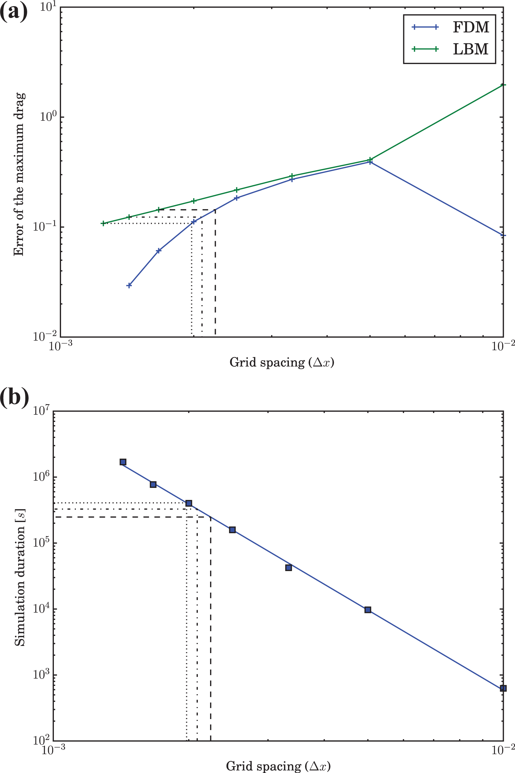
The process of interpolated simulation timings for the FDM using the LBM’s best maximum drag results. (a) Error of the maximum drag in relation to the FEM reference solution. Highlighted are the three LBM solutions on the finest mesh and the interpolated FDM equivalent. (b) Interpolated simulation duration for the FDM using a double logarithmic fit and the interpolated grid spacings.

Table 13.

The error in the maximum drag for the three finest resolutions of the LBM and the corresponding interpolation of the spatial resolution and simulation duration of the FDM.

	LBM		FDM (interpolated)		Runtime ratio
Error	$\Delta x$	Duration [s]	$\Delta x$	Duration [s]
0.1437	0.002	69822	0.00224	247940	3.55
0.1233	$0.001\overline{6}$	162050	0.00209	327492	2.02
0.1080	0.00125	275639	0.00198	407260	1.48

Considering only the computational throughput the above results are unexpected, as the FDM is capable of higher update rates at identical numbers of lattice sites. The deciding factor that causes the FDM to be significantly slower are the number of time steps. For the highest resolution case provided in Table 13 the time step sizes are 31.2 µs and 9.3 µs for the LBM and FDM, respectively.

Factors other than the reachable error and total runtime are also relevant and given in the following. Some of these figures, such as memory requirements, may even be crucial when dealing with limited hardware resources. Especially with regard to memory usage the FDM performs very well, requiring only 17 GiB for the 581 million DOF for the finest mesh at a spacing of 0.00143. The simulation ran on a single node for a total of 3116 CPU hours. The LBM is capable of running an even finer grid at a cell spacing of 0.00125 using only 2144 CPU hours on a single node. However, due to the nature of LBMs the 872 million DOF in terms of velocity and pressure are really 4142 million density distribution functions. The memory requirements are correspondingly larger at 90.8 GiB. For reference the resource consumption for the FEM based reference simulation is also provided, even though its implicit nature does not allow for a direct comparison. The mesh is locally refined in three levels leading to a minimal element length of 0.00079 and a total of 447 million DOF. The memory requirement of 1.2 TiB is significantly larger than for the explicit approaches and requires the simulation to be distributed between 24 nodes. It used a total of 4608 CPU hours.

4. Discussion

It is clear from the above results that the two methods are very similar in many respects. This includes their convergence behavior, artifacts from the weakly compressible nature and also the performance. However, the performance is a very sensitive measure and can vary greatly with regard to the specific problem setup and evaluated quantity. These fluctuations can span more than an order of magnitude either way and increase with the complexity of the test case and for derived flow quantities, such as overall lift and drag rather than velocity or pressure at specific points. Extracting a clear performance advantage for either approach is not possible, but nevertheless some important tendencies can established.

The two most significant tendencies correlate with the size of the desired error and whether derived quantities or the direct flow variables are inspected. Overall, a performance advantage for the LBM at coarse tolerances and for indirect measures, as well as an advantage for the FDM for strict tolerances and direct error measurements in velocity and pressure terms can be observed. This is supported by the findings from the three test cases.

The duct flow has the simplest setup and offers an analytical solution for the direct evaluation of the error in velocity and pressure profiles. Consistent with the trends postulated above, the LBM is competitive for the coarsest target tolerance, while the FDM exhibits a considerably better performance for the stricter tolerances. There the FDM can increase the performance advantage from a factor of 3.2 to 5.5 with increasing strictness.

The lid driven cavity has a more complex setup and flow pattern. Additionally, the error evaluation has to be carried out against a very high resolution reference result. The fact that for this test case both approaches are much closer performance-wise is in agreement with the postulated trends. The FDM starts out at being 1.3 times faster for the coarse tolerance, which increases to a factor of 2.2 at the strictest tested tolerance. The increase in the performance advantage for the FDM again underlines its better suitability for higher accuracy.

The transient test case of a flow past a cylinder with square cross section exhibits the most complex flow patterns and the integral quantities of lift and drag are the most indirect measures used in this work. Matching the expectations of the tendencies introduce above, the LBM has a much lower time to solution. Concerning the accuracy of the lift coefficient, the LBM outperforms the FDM by a factor of about 300. The results are less dramatic for the temporal development of the drag coefficient. A quantification of the total time to solution for the maximum of the drag coefficient resulted in a factor of 3.55 for a larger and of 1.48 for a smaller error between the FDM and LBM. Further refinements would be necessary for the FDM to draw equal to the LBM.

A further observation, which is most apparent with the test case of the flow past a cylinder, is the occasional difficulty to reach the reference solution with the LBM. The solution for the lift coefficient quickly overshoots past the reference and thus limits the capability of the LBM to reduce the error. This effect causes the FDM to ultimately catch up performance-wise, independent of the initial situation for coarser meshes.

Apart from the undecided performance question, other secondary factors go into the practicability of a method as well. The LBM has the advantage of very simple equations that are easily implemented and easily tuned, also automatically. For the evaluation of the domain, no additional parameters are required and the method is inherently stable within certain bounds. Furthermore, the LBM takes fewer time steps than the FDM for the examples considered here. The difficulty lies in the boundary conditions, as there is no well-established choice to apply simple boundary conditions accurately. These accuracy problems are computationally expensive to overcome. Additionally, the density distribution functions are difficult to interpret directly, which makes the analysis of the physical behavior of boundary conditions in general, and for corner cases in particular, even more difficult. The high number of distributions also increases the memory footprint and places a high load on the memory bandwidth.

The FDM excels due to the straight forward application of boundary conditions and the direct use of velocity and pressure, making it easy to interpret the behavior of the method. The difficulty lies in the evaluation of the domain itself. This is due to a very complex kernel and the necessity for stabilization techniques, including their effect on the maximal admissible time step size. The stabilization can require additional parameters that allow or require tuning to achieve stability and a high performance. Tests in running the duct flow example with stabilization parameters from an educated guess resulted in a 1.4–2.4 times longer evaluation for the coarse and fine tolerances respectively.

5. Conclusion and outlook

In this work a performance comparison between highly tuned LBM and FDM codes was carried out. The objective was to establish whether one approach is generally more efficient than the other at solving incompressible flow problems. The choice of methods was driven by comparability considerations and the test cases were matched up to the methods capabilities in order to produce fair results.

The free simulation parameters were optimized for the chosen codes, test cases and tolerances, and the resulting maximized performance was measured. From the results no definite performance advantage for either approach could be established, as they are very close. However, some overall trends were observed. The LBM tends to exhibit the higher performance for more complex problems, coarser tolerances and indirect benchmark quantities, such as lift and drag forces derived from the flow. The strength of the FDM lies in stricter tolerances and for direct evaluation of velocity and pressure values. Regarding the performance for the same number of lattice points, the FDM can be evaluated more quickly due to a lower memory transfer of the four quantities of velocity and pressure in each grid point, compared to the 19 distribution functions of the LBM. On the other hand, the LBM typically involves fewer time steps. Which method is in fact faster depends on the specific circumstances.

In the process of the performance assessment an additional aspect, relevant in engineering in particular, was observed. The LBM is fairly simple to set up with regards to the simulation parameters, as no supplementary parameters require tuning. Instead the difficulties arise in the choice of BCs, which is not as straight forward as for the FD approach and can severely reduce the accuracy of the results. The FDM on the other hand requires tuning of stabilization parameters, a suboptimal choice of which can cause either performance penalties or inaccurate results.

Further expanding the set of tests and parameters by the most promising candidates is subject to future investigations, as is a successive increase in both methods’ complexities toward current standards. These topics lead to enormous sets of design choices and restrictions to be assessed. Yet, the present results covering both steady cases and a transient one provide a very important baseline also for other configurations than the ones considered here. Given the similar accuracy trends, progress in terms of more sophisticated numerical methods on either side, such as better collision models or better lattices for the LBM or higher order finite difference stencils, can be quantified in terms of their advantage of the simple models considered here. Finally, the results allow to quantify accuracy over performance also for other discretization schemes, such as high performance discontinuous Galerkin (Fehn et al., 2019) or flux reconstruction (Loppi et al., 2018) methods.