Analytic performance modeling and analysis of detailed neuron simulations

Abstract

Big science initiatives are trying to reconstruct and model the brain by attempting to simulate brain tissue at larger scales and with increasingly more biological detail than previously thought possible. The exponential growth of parallel computer performance has been supporting these developments, and at the same time maintainers of neuroscientific simulation code have strived to optimally and efficiently exploit new hardware features. Current state-of-the-art software for the simulation of biological networks has so far been developed using performance engineering practices, but a thorough analysis and modeling of the computational and performance characteristics, especially in the case of morphologically detailed neuron simulations, is lacking. Other computational sciences have successfully used analytic performance engineering, which is based on “white-box,” that is, first-principles performance models, to gain insight on the computational properties of simulation kernels, aid developers in performance optimizations and eventually drive codesign efforts, but to our knowledge a model-based performance analysis of neuron simulations has not yet been conducted. We present a detailed study of the shared-memory performance of morphologically detailed neuron simulations based on the Execution-Cache-Memory performance model. We demonstrate that this model can deliver accurate predictions of the runtime of almost all the kernels that constitute the neuron models under investigation. The gained insight is used to identify the main governing mechanisms underlying performance bottlenecks in the simulation. The implications of this analysis on the optimization of neural simulation software and eventually codesign of future hardware architectures are discussed. In this sense, our work represents a valuable conceptual and quantitative contribution to understanding the performance properties of biological networks simulations.

1. Introduction and related work

1.1. Neuron simulations

Understanding the biological and theoretical principles underlying the brain’s physiological and cognitive functions is a great challenge for modern science. Exploiting the greater availability of data and resources, new computational approaches based on mathematical modeling and simulations have been developed to bridge the gap between the observed structural and functional complexity of the brain and the rather sparse experimental data, such as the works of Izhikevich and Edelman (2008), Potjans and Diesmann (2012), Markram et al. (2015), and Schuecker et al. (2017).

Simulations of biological neurons are characterized by demanding performance and memory requirements: a neuron can have up to 10,000 connections and must track separate states and events for each one; the model for a single neuron can be very detailed itself and contain up to 20,000 differential equations; neurons are very dense, and a small piece of tissue of roughly 1 mm³ can contain up to 100,000 neurons; finally, very fast axonal connections and current transients can limit the simulation timestep to 0.1 ms or even lower. Therefore, developers have gone to great lengths optimizing the memory requirements of the connectivity infrastructure in Jordan et al. (2018), the efficiency of the parallel communication algorithm in Hines et al. (2011) and Ananthanarayanan and Modha (2007), the scalability of data distribution in Kozloski and Wagner (2011) and even the parallel assembly of the neural network in Ippen et al. (2017). While these efforts improve the performance of the distributed simulations, little is still known about the intrinsic single-core and shared-memory performance properties of neuron simulations. On the other hand, the work of Zenke and Gerstner (2014) studied the performance of shared-memory simulations of biological neurons. However, their analysis is mainly based on empirical performance analysis and is centered on current-based point neuron simulations, a formalism that discards information about a neuron’s arborization.

The assumptions underlying brain simulations are very diverse, leading to a wide range of models across several orders of magnitude of spatial and time scales and thus to a complex landscape of simulation strategies, as summarized in the reviews by Brette et al. (2007) and Tikidji-Hamburyan et al. (2017). In this work, we focus on the simulation of morphologically detailed neurons based on the popular neuroscientific software NEURON presented in Carnevale and Hines (2006), which implements a modeling paradigm that includes details about a neuron’s individual morphology as well as its connectivity and allows to easily introduce custom models in the system. Our purpose is to extract the fundamental computational properties of the simulations of detailed biological networks and understand their relationship with modern microprocessor architectures.

1.2. The need for analytic performance modeling

An analytic performance model is a simplified description of the interactions between software and hardware together with a recipe for generating predictions of execution time. Such a model must be simple to be tractable but also elaborate enough to produce useful predictions.

Purely analytic (aka first-principles or white-box) models are based on known technical details of the hardware and some assumptions about how the software executes. The textbook example of a white-box model is the Roofline model by Williams et al. (2009) for loop performance prediction. The accuracy of such predictions depends crucially on the reliability of low-level details. A lack of predictive power challenges the underlying assumptions and, once corrected, often leads to better insight.

Black-box models, on the other hand, are ideally unaware of code and hardware specifics; measured data are used to identify crucial influence factors for the metrics to be modeled (see e.g. Calotoiu et al., 2013). One can then predict properties of arbitrary code or play with parameters to explore design spaces. Black-box models have a wider range of applicability: Even if low-level hardware information is lacking, they still provide predictive power. Wrong predictions, however, may be rooted in inappropriate fitting procedures and do not directly lead to better insight.

In this work, we choose the analytic approach combined with some phenomenological input, which makes the model a gray-box model. Analytic modeling has several decisive advantages that make it more suitable for delivering the insight we are looking for. First, it allows for universality identification, which means that some behavior in hardware–software interaction is valid for a wide range of microarchitectures of some kind. Second, it enables the identification of governing mechanisms: Since the model pinpoints the actual performance bottlenecks in the hardware, classes of codes with similar behavior are readily identified. This insight directly leads to possible codesign approaches. And third, analytic models provide insight via model failure, as described above.

1.3. The ECM performance model for multicore processors

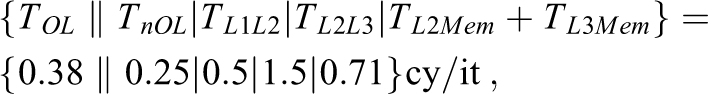
The Execution-Cache-Memory (ECM) model takes into account predictions of single-threaded in-core execution time and data transfers through the complete cache hierarchy for steady-state loops. These predictions can be put together in different ways, depending on the CPU architecture. The following steps must be taken to set up the model for a given sequential loop code on a given architecture:

Calculate data transfer volumes per iteration across the memory hierarchy, that is, for all data paths. This requires knowledge about how the data flows through the system and how the caches are organized (i.e. inclusive vs. exclusive). It is simple to do for pure streaming kernels with only spatial data locality but could become involved for kernels with data reuse. See, for example, Hager et al. (2018).

Using the known data path bandwidths $\left\{b_i\right\}$ , calculate the data transfer times across all data paths $\left\{i\right\}$ :

$T_i=\frac{V_i}{b_i}\mathrm{.}$

1

Here, V_i is the data volume transferred per iteration over data path i. Latency effects are ignored in this step, so these times are “optimistic.” For convenience, we use a compact notation for such predictions, for example:

$\{T_{L1L2}|T_{L2L3}|T_{L3Mem}\}=\{4|8|18.4\}\text{\hspace{0.05em}cy/it\hspace{0.17em}}\mathrm{.}$

2

3. Set up a model for execution time of the loop code, assuming that all data reside in the L1 cache. This is based on the compiler-generated machine code. It may be as simple as assuming maximum throughput for all instructions (relying on the out-of-order execution capabilities of the core to ensure maximum overlap among successive loop body executions) or as complex as considering the full critical path (CP). Tools such as IACA, the Architecture Code Analyzer by Intel (2017), ¹ can help with this task. It turns out that splitting the predicted execution time into data transfer cycles, specifically cycles in which loads retire (called “nonoverlapping time” $T_{nOL}$ ), and execution cycles, that is, all others (called “overlapping time” $T_{OL}$ ). Note that the model cannot determine if the compiler-generated code is “optimal.” This is still the task of an analyst who may, for example, notice that a specific loop was not vectorized although it should be. In this work, we used manual inspection on the compiler-generated code. Deficiencies will be pointed out if necessary.

4. The calculated time contributions must now be combined according to a machine model appropriate for the architecture at hand. As shown by Hofmann et al. (2018), different CPUs can have different machine models, but the crucial feature of a machine is its ability to overlap data transfers in the memory hierarchy. On all recent Intel server microarchitectures, it turns out that the single-core model yields the best predictions if one assumes no temporal overlap of data transfers through the cache hierarchy and between the L1 cache and registers (i.e. $T_{nOL}$ ), while the remaining in-core execution (such as arithmetic or any pipeline bubbles) shows full overlap.

The necessary information about the processor to construct the ECM model, for example, data path bandwidths, the number, throughput, and latency of execution units, the organization of the caches, and so on can ideally be obtained from vendor documentation such as Intel (2018). If such information is unavailable or incomplete, as is usually the case for the overlapping characteristics of the memory hierarchy, microbenchmarks can be used. See Hofmann et al. (2019) for a full account of the necessary procedures.

For a data set in main memory on one core of an Intel server CPU with an inclusive cache hierarchy, the model thus predicts the following per-iteration loop runtime:

$T_{ECM}^{Mem}=\text{max}\left(T_{OL},T_{nOL}+T_{L1L2}+T_{L2L3}+T_{L3Mem}\right)\mathrm{.}$

3

Here, $T_{OL}$ is the part of the in-core execution that is unrelated to data transfers, such as arithmetic, while $T_{nOL}$ is the time (cycles) required to retire load instructions. Now it becomes evident why the in-core execution must be split into the $T_{nOL}$ and $T_{OL}$ contributions: $T_{nOL}$ counts as data transfer and does not overlap with the rest of the transfers through the cache hierarchy, while $T_{OL}$ is work, such as floating-point and integer arithmetic, which can be carried out independently. The model (3) can be used for working sets that are not in main memory by omitting all memory hierarchy levels that do not source or sink data; for example, for a data set that fits in L3 cache, $T_{L3Mem}=0$ . In (2) we introduced a compact notation for writing the individual time contributions for the model. For the actual runtime predictions, which emerge from (3), we use the following shorthand notation, to be distinguished from (2) by the use of ⌉ as delimiter:

$\left\{T_{ECM}^{L1}\rceil T_{ECM}^{L2}\rceil T_{ECM}^{L3}\rceil T_{ECM}^{Mem}\right\}\text{\hspace{0.17em}\hspace{0.05em}\hspace{0.17em}cy/it\hspace{0.05em}},$

4

where $T_{ECM}^X$ denotes the runtime prediction if data comes from the Xth level of the memory hierarchy. The delimiter symbolizes the fact that time contributions from all memory hierarchy levels up to the one given on its left are considered for putting together the prediction. For presenting measurements, we substitute the curly braces with parentheses or omit them altogether.

Scalability across cores is assumed to be perfect until a bandwidth bottleneck is hit. Since the memory interface is the only multicore bandwidth bottleneck on Intel processors, the predicted execution time is for n cores is

$T_{ECM}=\text{max}\left(\frac{T_{ECM}^{Mem}}{n},T_{L3Mem}\right)\mathrm{.}$

5

The bandwidth saturation point, that is, the number of cores required for saturation, is readily obtained from this expression:

$n_S=\lceil \frac{T_{ECM}^{Mem}}{T_{L3Mem}}\rceil$

6

A full account of the ECM model would exceed the scope of this article, so we refer to Stengel et al. (2015) and Hofmann et al. (2019) for a recent discussion. Note that IACA was used for the in-core analysis part of all the loops investigated in this article. The data transfer part was straightforward to set up since no significant temporal data reuse occurs. Difficulties encountered with the modeling procedures will be pointed out where relevant. An example of how the ECM model can be constructed for a simple streaming kernel will be given in Section 2.1.

Up to now, the ECM model has been shown to work well for standard multicore CPUs. Extension of the model to accelerators, specifically GPGPUs, is under investigation. The main problem with these kinds of architectures is that latency effects play a major role for single-core/thread execution, but they are ignored by the model in its current form.

1.4. Contributions and organization of this article

In this work, we make the following contributions:

We demonstrate that the analytic ECM performance model can be applied successfully to nontrivial loop kernels with a wide range of different performance features. Although there are considerable error margins in some cases, a very good qualitative understanding can be achieved.

We identify cases where the model needs corrections or cannot be applied sensibly: strong latency components in the data transfers and long CPs in the core execution. While latency-bound data access is beyond the applicability of the model in its current form, a long CP does not hinder the derivation of useful qualitative conclusions.

We apply the ECM model for the first time to the Intel Skylake-X processor architecture, whose cache hierarchy is different from earlier Intel designs.

We give clear guidelines for codesigning an “ideal” processor architecture for neuron simulations. In particular, we spot wide SIMD capabilities as a crucial ingredient in achieving memory bandwidth saturation. A low core count part with a high clock speed and wide SIMD units (such as AVX-512) will present the most cost-effective hardware platform. Cache size is inconsequential for most kernels.

This article is organized as follows: In section 2, we give details on the software and hardware environment under investigation, including preliminary performance observations. In section 3, we construct and validate ECM performance models for the important kernel classes in NEURON. In section 4, we summarize and discuss the findings in order to pinpoint the pivotal components of processor architectures in terms of neuron simulation performance and give an outlook to future work.

We provide a reproducibility appendix as a downloadable release file at Cremonesi et al. (2019), which should enable the interested reader to rerun our experiments and reproduce the relevant performance data.

2. Application and simulation environment

2.1. Target architectures and programming environment

We apply the ECM model introduced by Treibig and Hager (2010) and refined by Stengel et al. (2015) on two Intel processors with different micro-architectures: the Ivy Bridge (IVB) Intel(R) Xeon(R) E5-2660v2 and the Skylake (SKX) Intel(R) Xeon(R) Gold 6140 (with Sub-NUMA clustering turned off). The ECM model for the IVB architecture has been extensively studied by Hofmann et al. (2017) and Hammer et al. (2017). The ECM model for the SKX architecture has not been fully developed to date, but a preliminary formulation based on (5) that takes into account the victim cache architecture of the L3 was published in Hager et al. (2018). The heuristics governing cache replacement policies are not disclosed by Intel, but we have found that the following assumptions usually lead to good model predictions:

Read traffic from main memory goes straight to L2.

All evicted cache lines from L2, both clean and dirty, are moved to L3.

The data path between the L2 and the L3 cache can be assumed to provide a bandwidth of 16 B/cy in both directions (i.e. full duplex).

The most relevant hardware features for the modeling of both architectures are presented in Tables 1 and 2. The Intel IACA tool was used for estimating in-core execution times of loop kernels. Although IACA supports both architectures, its support for CP prediction was recently dropped. The IACA outputs for all kernels are available in the reproducibility appendix.

Table 1.

Hardware characteristics of the target CPU architectures.

Characteristic	IVB	SKX
CPU freq (GHz)	$2.2$	$2.3$
Uncore freq (GHz)	$2.2$	$2.3$
Mem BW (meas.) (GB/s)	$40$	$105$
LD/ST throughput per cy:
AVX(2), AVX512	1 LD, $\frac{1}{2}$ ST	2 LD, 1 ST
SSE, scalar	2 LD $||$ 1 LD, 1 ST	2 LD, 1 ST
AGUs	2	2 + 1 simple
Per-core L1–L2 BW (B/cy)	$32$	$64$
Per-core L2–L3 BW (B/cy)	$32$	$2\times 16$
Compiler	Intel 17.0.1	Intel 18.0.1
IACA version	2.1	3.0

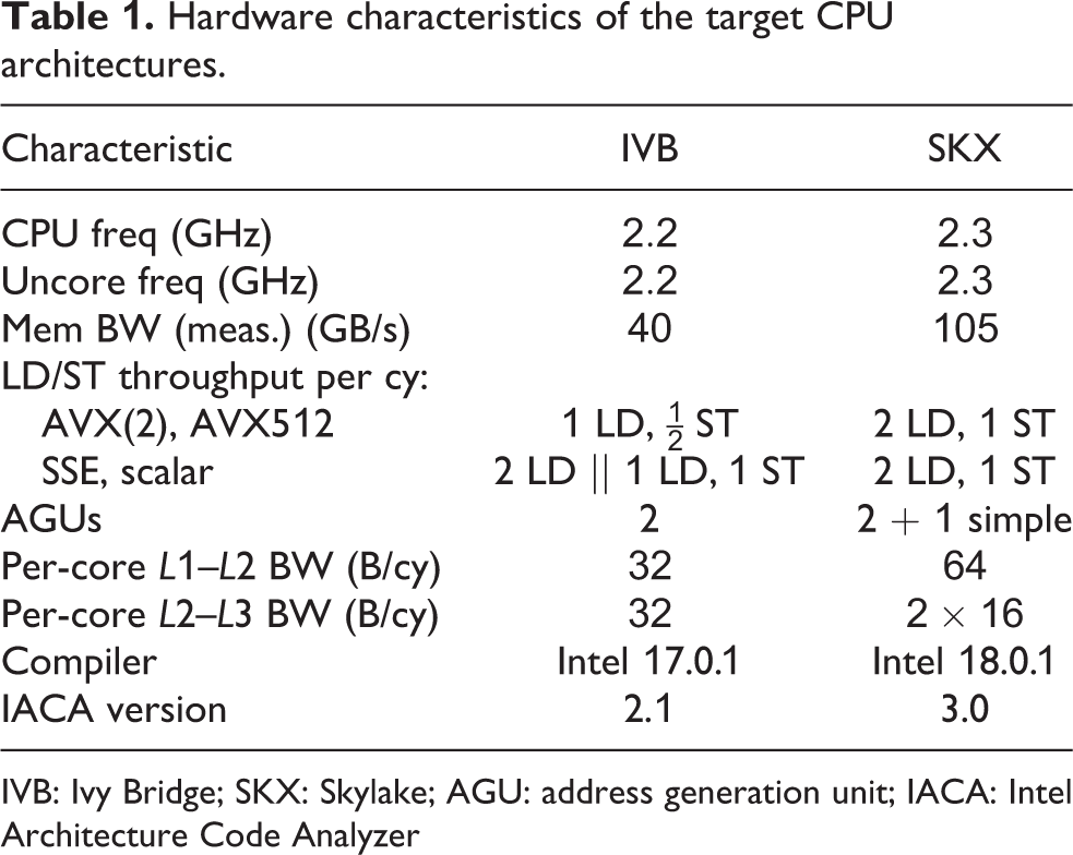
IVB: Ivy Bridge; SKX: Skylake; AGU: address generation unit; IACA: Intel Architecture Code Analyzer

Table 2.

Useful benchmark values (double precision).^a

Inverse throughput	IVB		SKX
(lr)2–3 (lr)4–6 for	SSE	AVX	SSE	AVX	AVX512
Vector exp() [cy]	11.5	8.0	6.7	3.5	1.5
Vector div 2 [cy]	7	7	2	2	2
Scalar exp() [cy]	27.8		15.1

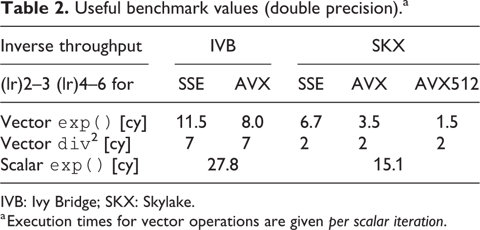
IVB: Ivy Bridge; SKX: Skylake.

^a Execution times for vector operations are given per scalar iteration.

We illustrate the application of the ECM model to SKX with the STREAM triad kernel developed by McCalpin (1995):

$\text{A(:)=B(:)}+\text{k*C(:)}.$

7

Considering only AVX vectorization as an example, this kernel has the following properties per scalar iteration:

Inverse throughput prediction of $T_{OL}=0.375\text{\hspace{0.17em}cy/it}$ , bound by address generation units (AGUs).

Two loads and one store, so $T_{nOL}=0.25\text{\hspace{0.17em}cy/it}$ .

$V_{L1L2}=32\text{\hspace{0.17em}B/it}$ (including write-allocate).

$T_{L1L2}=\frac{32\text{\hspace{0.05em}\hspace{0.17em}B/it}}{64\text{\hspace{0.05em}\hspace{0.17em}B/cy}}=0.5\text{\hspace{0.17em}cy/it}$ .

Due to the victim L3 cache, we have to distinguish in-memory and in-L3 data sets.

L3: $V_{L2L3}^{L3}=48\text{\hspace{0.17em}B/it}$ (read + write).

Memory: $V_{L2L3}^{Mem}=24\text{\hspace{0.17em}B/it}$ (write-only).

The transfer times between L2 and L3 are the same in this particular case because reads and writes to L3 can overlap:

L3: $T_{L2L3}^{L3}=\text{max}\left(\frac{24\text{\hspace{0.17em}\hspace{0.05em}B/it}}{16\text{\hspace{0.05em}\hspace{0.17em}B/cy}},\frac{24\text{\hspace{0.05em}\hspace{0.17em}B/it}}{16\text{\hspace{0.05em}\hspace{0.17em}B/cy}}\right)=1.5\text{\hspace{0.17em}cy/it}$ .

Memory: $T_{L2L3}^{Mem}=\frac{24\text{\hspace{0.17em}\hspace{0.05em}B/it}}{16\text{\hspace{0.05em}\hspace{0.17em}B/cy}}=1.5\text{\hspace{0.17em}cy/it}$ (write-only).

$V_{L2Mem}=24\text{\hspace{0.17em}B/it}$ (read-only traffic).

$T_{L2Mem}=\frac{24\text{\hspace{0.17em}\hspace{0.05em}B/it}}{105\text{\hspace{0.05em}\hspace{0.17em}GB/s}}\times 2.3\text{\hspace{0.17em}\hspace{0.05em}Gcy/s}=0.53\text{\hspace{0.17em}cy/it}$ .

$V_{L3Mem}=8\text{\hspace{0.17em}B/it}$ (write-only traffic).

$T_{L3Mem}=\frac{8\text{\hspace{0.05em}\hspace{0.17em}B/it}}{105\text{\hspace{0.17em}\hspace{0.05em}GB/s}}\times 2.3\text{\hspace{0.17em}\hspace{0.05em}Gcy/s}=0.18\text{\hspace{0.17em}cy/it}$ .

So the ECM model contributions for the STREAM triad kernel in (7) on SKX-AVX would be:

$\begin{array}{l}\left\{T_{OL}\parallel T_{nOL}|T_{L1L2}|T_{L2L3}|T_{L2Mem}+T_{L3Mem}\right\}=\\ \left\{0.38\parallel 0.25|0.5|1.5|0.71\right\}\text{cy/it\hspace{0.05em}\hspace{0.17em}},\end{array}$

with corresponding predictions according to the nonoverlapping machine model of $\left\{0.38\text{⌉}0.75\text{\hspace{0.05em}⌉}2.25\text{⌉}2.96\right\}\text{\hspace{0.05em}cy/it}$ . For validation we compared these predictions to benchmark measurements and obtained $\left(0.39\text{⌉}0.73\text{⌉}2.37\text{⌉}4.3\right)\text{\hspace{0.05em}cy/it}$ , which is in reasonable agreement with the model. The deviation in memory could be fixed by introducing a latency penalty (see Hofmann et al., 2017), but since the memory contribution is rather small for most of the kernels studied here we opted for a simpler model. In this simple example, we have assumed a “perfect” machine code with the minimum number of instructions per scalar iteration. For the modeling of more complex kernels, we use the actual, unmodified assembly code as generated by the compiler.

To roughly compare the two architectures, a common approach is to use the peak performance as a metric, measured in single-precision or double-precision Gflop/s. The IVB chip supports AVX vectorization and can retire one multiply and one add instruction per cycle, while the SKX chip supports AVX512 vectorization and can retire two fused multiply-add instructions per cycle. This leads to the peak performance numbers as shown in Table 3. The naive Roofline model uses the peak performance of the chip as the core-bound limit, but often other limitations apply, such as the load or store throughput between registers and the L1 cache, or pipeline stalls due to a long CP or loop-carried dependencies. The ECM model takes this into account via the $T_{nOL}$ and $T_{OL}$ runtime contributions, which are based on an analysis of the actual loop code.

Table 3.

Peak performance for the target architectures.

Architecture	Formula	DP $P_{peak}$ (Gflop/s)
IVB 1 core	$2.2\times 4\times 2$	17.6
SKX 1 core	$2.3\times 8\times 2\times 2$	73.6
IVB 1 socket	$10P_{peak}(1\text{core})$	176
SKX 1 socket	$18P_{peak}(1\text{core})$	1324.8

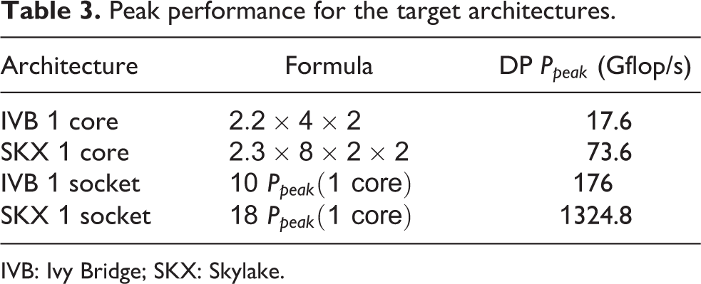
IVB: Ivy Bridge; SKX: Skylake.

On IVB, we used the Intel 17.0.1 compiler with options -xSSE4.2 and -xAVX for SSE and AVX code, respectively. On SKX, we used the Intel 18.0.1 compiler with options -xSSE4.2, -xAVX2, and -xCORE-AVX512 -qopt-zmm-usage=high for SSE, AVX, and AVX512 code, respectively. On both machines, we employed #pragma ivdep, #pragma vector aligned, and #pragma omp simd simdlen(N) directives where appropriate to ensure vectorization. The compiler option -qopt-streaming-stores never was used to disable the generation of nontemporal stores by the compiler.

To measure relevant performance metrics such as data transfer through the memory hierarchy, we used the likwid-perfctr tool from the well-established LIKWID framework presented by Treibig et al. (2010) and Gruber et al. (2018). We instrumented the code using markers and inserted a barrier before the execution of each kernel to ensure that measurements would be minimally affected by load imbalance. This is actually close to a real-world usage scenario, because any load imbalance would have to be corrected via dynamic or guided OpenMP loop scheduling, which would necessitate barrier synchronization between adjacent loops. The overhead caused by the barrier itself was insignificant compared to the kernels’ runtime. On both architectures, we employed the CACHES performance group and pinned the OpenMP threads to the physical cores of a socket. In order to guarantee reproducible benchmark runs, we employed the likwid-setFrequencies tool to set the clock speed of the cores (and the Uncore in case of SKX) to the base values indicated in Table 1. In spite of this, we observed the well-known kernel-specific clock frequency throttling on the SKX architecture at all vectorization levels: the average clock frequency never exceeded the limits in Table 1 but in some kernels it was observed to be lower, although never less than 2.1 GHz. In the course of our analysis, we scale our performance predictions by the measured clock frequency whenever required.

2.2. Simulation of morphologically detailed neurons

A common approach to modeling morphologically detailed neurons is the so-called conductance-based (COBA) compartmental model as formalized in the reviews by Brette et al. (2007), Bhalla (2012), and Gerstner et al. (2014). In this abstraction, the arborization of dendrites and axons is represented as a tree of sections, where a section corresponds to an unbranched portion of the neuron. Each section is then divided into compartments that represent discretization units for the numerical approximation. Quantities of interest such as membrane potential or channel gating variables are typically only well defined at compartment centers and branching points.

In the compartmental model, each compartment is considered analogous to an RC circuit where the resistance (or rather, the conductance) term can be nonlinearly dependent on the membrane potential itself. Due to their stability, implicit methods are a common choice for time integration of the differential equations arising from this representation, thus the solution of a linear system of equations is required at each timestep. In the presence of branching points, this leads to a quasi-tridiagonal system that can be solved in linear time using the algorithm proposed in Hines (1984).

In the COBA model, the membrane conductance is determined by aggregating several contributions from ion channels, which are special cross-membrane proteins that allow an ionic current to flow into or out of the cell. Thus in the COBA compartmental model, when using an implicit time integrator, three algorithmic phases are required to advance a neuron in time: first one must compute the contributions to the linear system (the ion channel and synapses currents); then one must solve the linear system; finally, one must update the states of individual ion channel and synapse instances based on the recently computed compartment potentials (see Figure 1). Note that in this model each ion channel or synapse type will have two kernels associated with it: a current kernel that defines how to compute the contributions to the linear system for that family of ion channels or synapses, and a state kernel that defines the numerical time integration of that ion channel’s or synapse’s state variables, typically based on the exponential Euler method (see Oh and French, 2006).

Figure 1.

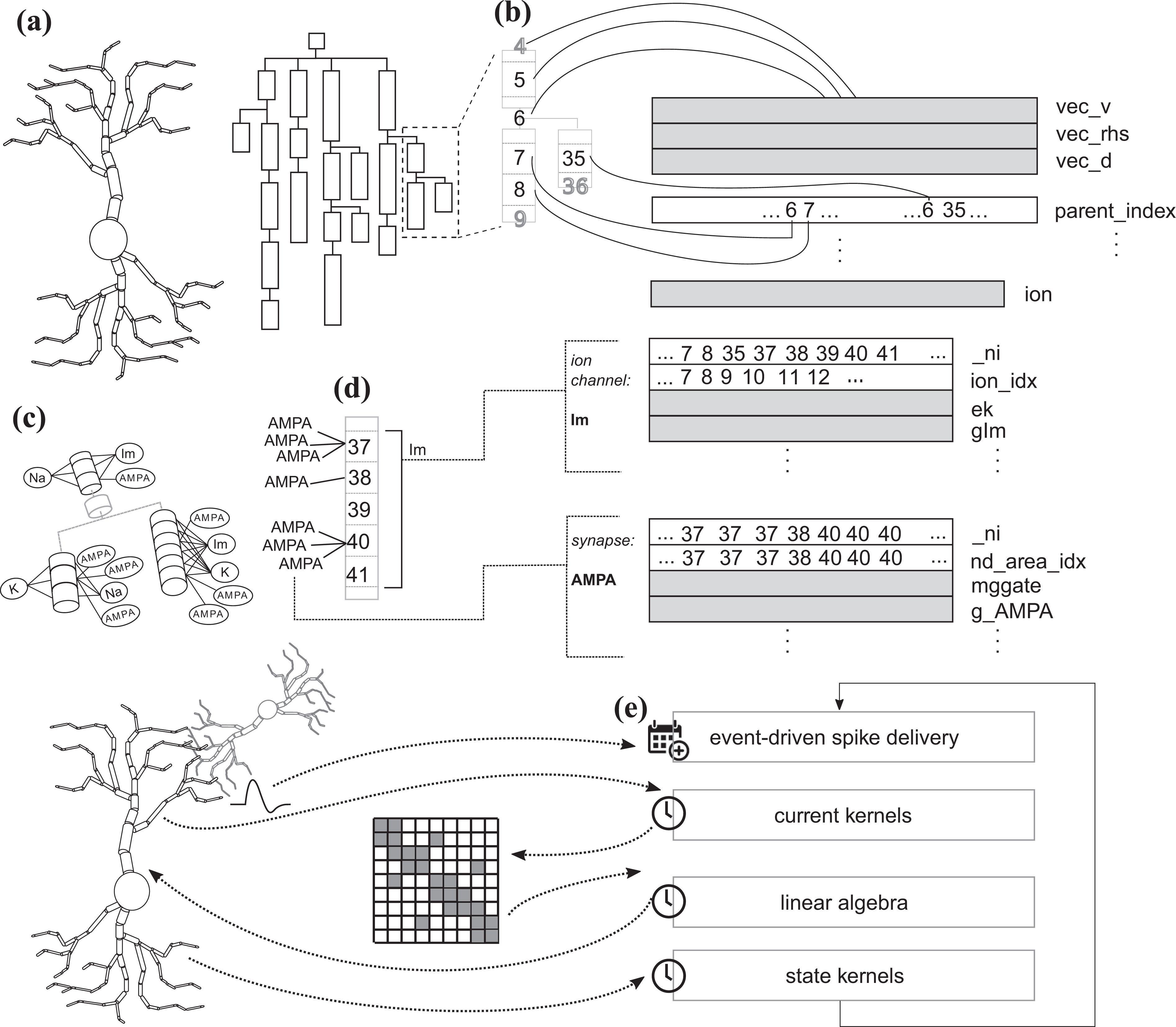
Neuron representation and data layout. (a) Neurons are represented as a tree of unbranched sections, where each section can be further split into compartments for numerical discretization. (b) Each compartment is numbered according to the schema in Hines (1984), and the tree structure is represented in memory by an array of parent_index. Additional arrays are used to represent the neuron’s state (e.g. vec_v holds the membrane potential of each compartment), and three arrays are used for a sparse representation of the time integration matrix. Arrays of double precision values are colored in grey, while arrays of integer indices are white and contain some elements to give an idea of their structure. (c) Additionally, every compartment can be endowed with zero or more ion channels or synapses, which require additional arrays to be represented. Branching points (in grey) are treated as any other compartments for the purposes of linear algebra, but do not have any instances of ion channels or synapses. (d) Ion channels (e.g. Im) either have a single instance in all the compartments of a section or do not have any instances at all in that section. Synapses (e.g. AMPA) can have multiple instances per compartment and do not need to be represented in all the compartments belonging to the same section. (e) The application’s workflow, excluding bookkeeping and parallel communication. First, the spike delivery kernel is called only for all the events that have been generated by other neurons and that have an effect on synapses of this neuron; then, at every timestep, the current, linear algebra and state kernels are executed. Current kernels read information from the state of the neuron and update the linear system’s matrix. Linear algebra solves the linear system using a custom method and updates the state of the membrane potential. State kernels read the membrane potential and update the state of all the ion channels and synapses.

Neurons also have the ability to communicate with other neurons using synapses: points of contact between different neurons that are triggered when an action potential is elicited in the presynaptic cell and, at the onset of this event, determine a change in the membrane potential of the postsynaptic cell. Therefore, the simulation algorithm is composed of two parts: a clock-driven portion that advances the state of a neuron from a timestep to the next; and an event-driven part that is only executed when a synaptic event is received. Figure 1 presents a summary of the main algorithm phases and data layout.

The compartmental modeling of neurons using COBA formalism is implemented in the widely adopted software for neuroscientific simulations NEURON. The NEURON software is a long-lasting project that includes an interpreter for a custom scripting language (HOC), a domain specific language tool to expand the models of ion channels and synapses, a GUI and a domain specific language (NMODL) to expand the repertoire of available models. To reduce the complexity and concentrate on the fundamental computational properties of the simulation kernels, in this work we utilize instead CoreNEURON, a lean version of NEURON’s simulation engine based on the work by Kumbhar et al. (2016). CoreNEURON implements several optimizations over NEURON, including improved memory requirements and vectorization, at the cost of functionality. In particular, NEURON is usually still required to define a model and a simulation setup before CoreNEURON executes the simulation. The NEURON/CoreNEURON software allows neuroscientists to specify custom ion channel and synapse models using the domain specific language NMODL introduced in Hines and Carnevale (2000), which is then automatically translated into C code and compiled in a dynamic library.

The CoreNEURON data layout is shown in Figure 1. First, the neuron is modeled logically as a tree of unbranched sections, whose topology is represented by a vector of parent indices. Other relevant quantities such as the membrane potential and the tridiagonal sparse matrix are represented by double precision arrays with length equal to the number of compartments. More details about the matrix representation are given in Section 3.6. Additionally, ion channel-specific and synapse-specific quantities are held in separate data structures consisting of arrays of double precision values in Structure-of-Arrays layout (SoA), indices to the corresponding compartments and, if needed, pointers to other internal data structures.

2.3. Preliminary performance observations and motivation

Given that the simulation algorithm is composed of many phases with different characteristics, the first step in performance analysis is a search for the time-consuming hot spots. We created a data set consisting of 500 replicas of a Layer 5 pyramidal neuron from the rat’s somatosensory cortex (see Ramaswamy et al., 2015). This type of neuron was chosen because it contains all of the most common ion channel and synapse types in a reconstruction of the cortical microcircuit (see Markram et al., 2015), while the number of replicas was chosen to ensure with absolute certainty that the corresponding data set would not fit in the L3 cache. Although the number of neurons in a data set primarily affects its size, and thus the level of memory where the working set resides, network size effects can come into play, changing the frequency at which neurons exchange synaptic events, thus changing the relative weight of the spike delivery function. However, such effects are difficult to predict and depend on many external factors such as random input noise and connectivity among neurons, therefore we chose to neglect this direction of analysis and kept the number of neurons fixed. To account for different data set sizes, in the detailed analysis of individual ion channels and synapses, we also consider smaller data sets that fit in the L3 and L2 cache. In the shared-memory parallel execution, current and state kernels are usually dominant, representing roughly 80% of the total execution time, while the event-driven spike delivery and linear algebra kernels account for less than 10% each (see Figure 2(a)). In the serial execution, we observe that the relative importance of spike delivery increases slightly, however, the state and current kernels still dominate. This serial performance profile was also observed in Kumbhar et al. (2016) and is a distinctive feature of compartmental COBA models, whereas current-based point neuron models are typically dominated in serial execution by event-driven spike delivery and event bookkeeping, as shown in the work by Peyser and Schenck (2015). Unfortunately, these results are tightly linked to the benchmark setup, and it is unknown whether this is a general property of COBA models or not.

Figure 2.

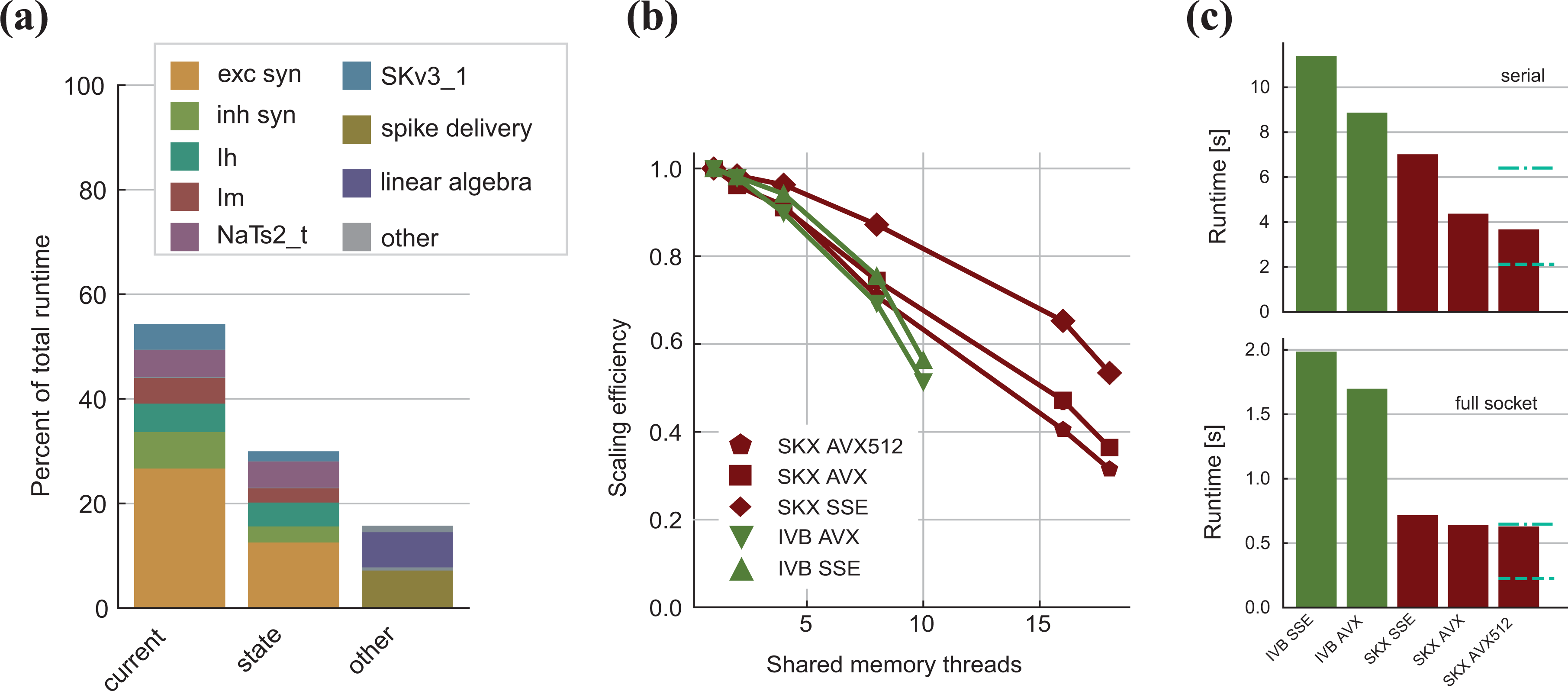
Measured performance and observations from benchmark. (a) Breakdown of the distribution of relative importance of the different kernels in the simulation of a full neuron for the SKX-AVX512 architecture using a full socket. Overhead from the rest of the execution is not shown. Linear algebra and spike delivery combined hardly exceed 10%. (b) Median strong scaling efficiency over 10 runs. Measurements exhibited little variability across different runs, so quantile error bars are not visible. Parallel efficiency degrades quickly, especially on SKX, and vectorization strengthens this negative effect. (c) Total runtime to simulate one neuron for one second in the serial case (top) and using the full socket (bottom). Overhead from the non-computational kernels is not considered. The dashed blue line represents the expected runtime if scaled perfectly with the architecture’s theoretical peak performance from IVB-AVX to SKX-AVX512, while the dash-dotted blue line marks the expected runtime if scaled perfectly with the ratio of measured memory bandwidths. We do not observe the ideal speedup, and in this article we employ performance modeling to explain the underlying reasons. IVB: Ivy Bridge; SKX: Skylake.

We have chosen two Intel architectures that were introduced about 5 years apart in order to be able to identify the speedup from architectural improvements. Judging by the peak performance numbers in Table 3, one would expect a per-socket speedup of about 7.5 $\times$ . On the other hand, comparing memory bandwidth (see Table 1), which is the other lowest order bottleneck of code execution, a factor of 2.6 $\times$ could be estimated. As shown in Figure 2(c), we observe a factor of roughly 3 $\times$ between the best IVB and SKX versions. Although it is satisfying that the measurement lies between the two estimates, detailed performance modeling is required to explain the actual value.

One of the main in-core features of modern architectures is the possibility to expose data parallelism using vectorized (SIMD) instructions on wide registers. We investigated the benefits of vectorization at different levels of thread-parallelism. In the serial execution (see Figure 2(c)), we found that the Skylake architecture had in general better performance than Ivy Bridge, and that using wider registers improved the performance, even though the acceleration was not ideal (i.e. not in line with the larger register width). At full socket, we found that the difference between architectures was exacerbated, while we saw only minor improvements from vectorization (see Figure 2(c)). We also investigated the strong-scaling efficiency of the simulation code on different architectures (Figure 2(b)) and found that, as expected, the efficiency decreases as the level of parallelism grows. This indicates a tradeoff in terms of chip and software design: further analysis is required to understand whether it is worth investing in SIMD or shared-memory parallelism, optimize for instruction level parallelism, out of order execution or a combination of all of these.

We exploit performance modeling techniques in order to gain insight into the interaction between the CoreNEURON simulation code and modern hardware architectures. This will allow us to answer the open performance questions above as well as to generalize to different architectures for future codesign efforts.

3. Performance modeling of detailed simulations of neurons

3.1. Ion channel current kernels

Ion channel current kernels are used in the simulation algorithm to update the matrix representing the voltage equation by computing contributions from the ionic current of different chemical species. We consider in this work four ion channel types that are among the most representative: Ih, Im, NaTs2_t, SKv3_1. In Listing 1, we show the code for the Im current kernel as an example; other kernels share similar memory access patterns and arithmetic operations with only minor changes.

Listing 1.

Im current kernel.

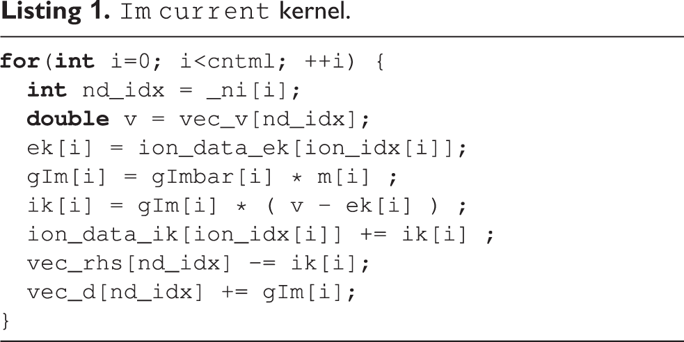
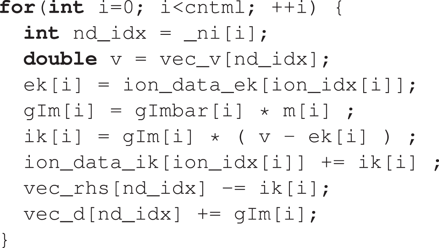
Current kernels are typically characterized by two main features: low arithmetic intensity and scattered loads/stores. The latter can present a modeling problem, but in practice we can obtain good accuracy using a few heuristics based on domain-specific knowledge. In particular, as a first approximation, one can treat the indices in _ni and ion_idx as perfectly contiguous (see Figure 1 as a justification). In total, the kernel reads from four double and two integer arrays, and writes to six double arrays, leading to 136 B of overall data traffic per scalar iteration through the complete memory hierarchy (this includes write-allocate transfers on store misses).

Combining the data volume estimates with in-core predictions from IACA (using the full throughput assumption), we can generate the ECM model predictions in cycles per scalar iteration as shown in Table 4. The compiler is able to employ scatter/gather instructions for this kernel on SKX (these are not supported on IVB). As expected, the model predicts that the performance of this strongly data-bound kernel will degrade as the data resides farther from the core. Vectorization is not beneficial at all except for AVX512 with data in L1, which can be attributed to the required scalar load instructions when gather/scatter instructions are missing. To validate the predictions, we designed a serial benchmark that allowed fine-grained control over the data set size by removing all ion channels and synapses except Im from our data set, but still executing the complete application loop. The resulting data set size was roughly 50 kB and 200 kB for the L2 benchmarks and 6 MB and 7 MB for the L3 benchmarks on the IVB and SKX architectures, respectively. Due to overheads, it was impossible to construct a benchmark for the L1 cache on either machine.

Table 4.

ECM model and serial measurements per scalar iteration (cy/it) for the Im current kernel.

	Contributions	Predictions	Measurements
IVB SSE	$\left\{7.8\parallel 5.5|4.2|4.2|7.5\right\}$	$\left\{7.8\text{⌉}9.7\text{⌉}13.9\text{⌉}21.4\right\}$	$\left(\text{n/a⌉}10.8\pm 0.1\text{⌉}13.5\pm 0.0\text{⌉}23.8\pm 0.1\right)$
IVB AVX	$\left\{7.8\parallel 5.6|4.2|4.2|7.5\right\}$	$\left\{7.8\text{⌉}9.8\text{⌉}14.0\text{⌉}21.5\right\}$	$\left(\text{n/a⌉}10.2\pm 0.0\text{⌉}13.1\pm 0.0\text{⌉}23.8\pm 0.2\right)$
SKX SSE	$\left\{7.8\parallel 5.5|2.1|5.5|3.0\right\}$	$\left\{7.8\text{⌉}7.8\text{⌉}13.1\text{⌉}16.1\right\}$	$\left(\text{n/a⌉}9.1\pm 0.1\text{⌉}11.0\pm 1.0\text{⌉}15.3\pm 1.0\right)$
SKX AVX	$\left\{7.3\parallel 4.8|2.1|5.5|3.0\right\}$	$\left\{7.3\text{⌉}7.3\text{⌉}12.4\text{⌉}15.4\right\}$	$\left(\text{n/a⌉}8.7\pm 0.1\text{⌉}11.4\pm 0.0\text{⌉}15.0\pm 1.2\right)$
SKX AVX512	$\left\{5.3\parallel 3.0|2.1|5.5|3.0\right\}$	$\left\{5.3\text{⌉}5.3\text{⌉}10.6\text{⌉}13.6\right\}$	$\left(\text{n/a⌉}7.6\pm 0.0\text{⌉}10.6\pm 0.8\text{⌉}15.6\pm 1.5\right)$

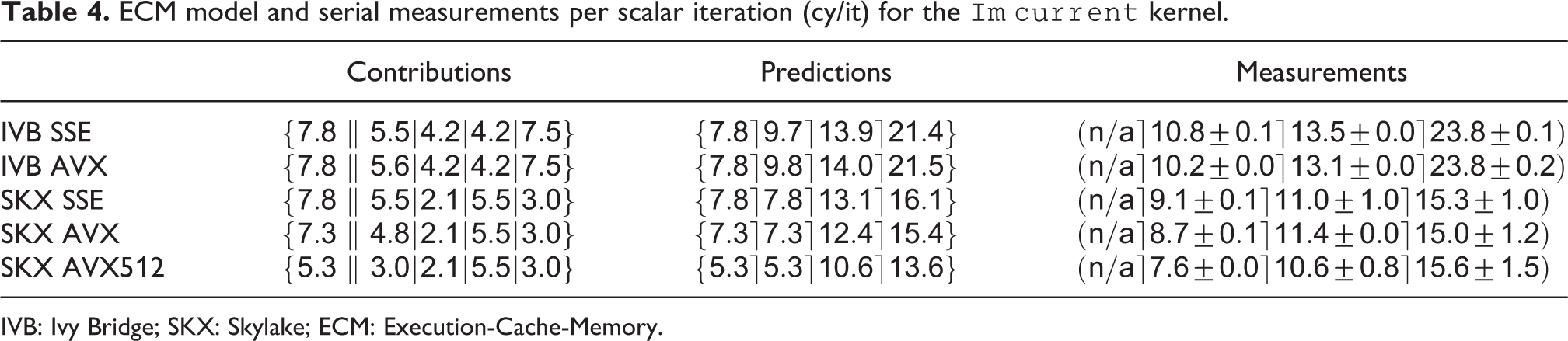
IVB: Ivy Bridge; SKX: Skylake; ECM: Execution-Cache-Memory.

On IVB, the measurements remained within 10% of the predictions for all levels of the memory hierarchy, while on SKX, the ECM predictions were a little more off, especially for data in the cache. This might be caused by our simplifying model assumptions about the data transfers between L2 and L3, for which no official documentation exists. Still the ECM model gave accurate predictions in almost all of our benchmarks and provided insight into the computational properties of this kernel.

We conclude that the Im current kernel, and all current kernels in general, are data-bound and limited solely by data transfer capabilities of the system across the memory hierarchy. Even for an in-memory data set, wider data paths between the caches would thus benefit the performance of the kernel. The clock frequency will have a significant but weaker than linear impact on the performance because memory transfer rates are only weakly dependent on it (especially on the more modern architectures like SKX). The analysis also predicts strong memory bandwidth saturation with a few (4–5) cores, so the memory bandwidth starts to play a decisive role once bandwidth saturation is achieved.

3.2. Synaptic current kernels

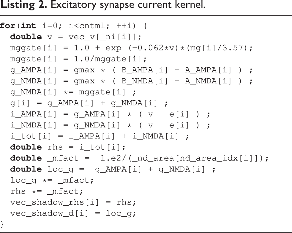
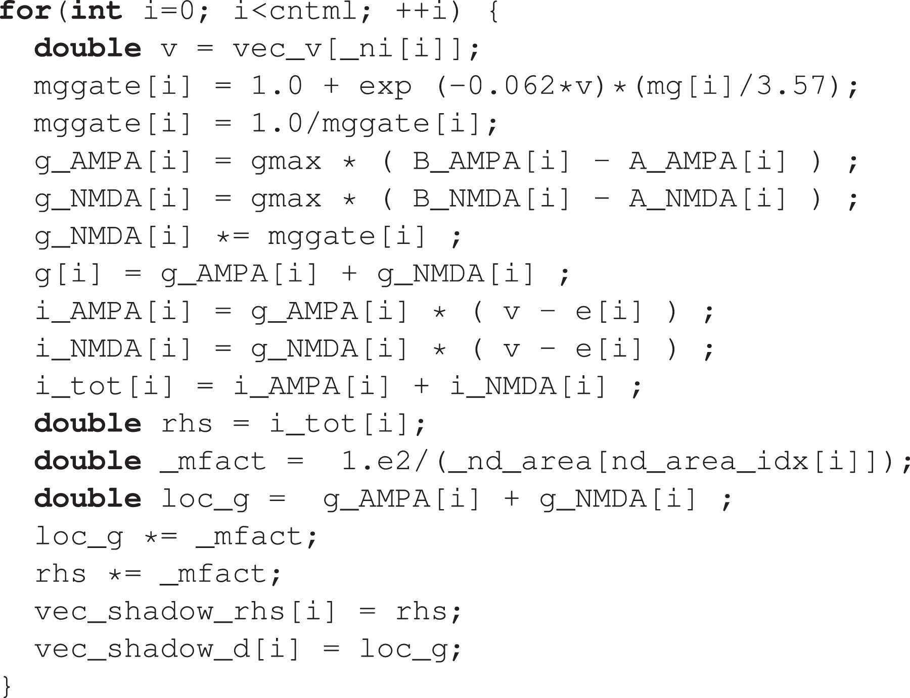
Synapses are arguably the pivotal component of neuron simulations. Synaptic current kernels are particularly important for performance as shown in Figure 2, and pose a modeling challenge because of their complex chain of intra-loop dependencies, memory accesses and presence of transcendental functions. There are two types of synapses in this data set: excitatory AMPA/NMDA synapses and inhibitory GABA-A/B synapses. As an example, the source code for the excitatory AMPA/NMDA synapse current is shown in Listing 2. The expensive exponentials and divides in this code are balanced by large data requirements. The kernel reads one element each from eight double and two integer arrays, and writes one element each to nine double arrays, which would amount to a traffic of 216 B per iteration. However, as shown in Figure 1, the typical structure of the _ni and nd_area_idx arrays is different from that of the indexing arrays in ion channel kernels. In particular, as a direct consequence of multiple synapse instances being able to coexist within the same compartment, the _ni and nd_area_idx arrays often exhibit sequences of repeated elements. This means that subsequent iterations of the kernel can exploit some temporal locality in accessing the vec_v and _nd_area arrays. To account for this, we reduce the expected traffic from these arrays by a weighting factor equal to the average length of a sequence of repeated elements in _ni and nd_area_idx, which is about 3 in our case. Thus the updated data traffic estimate is 205 B through the complete memory hierarchy. To compute $T_{OL}$ , the inverse throughput of the vectorized exponential operation from Table 2 must be added to the kernel runtime reported by IACA, and $T_{nOL}$ is derived from the retired load instructions as usual. We then obtain the ECM predictions per scalar iteration in Table 5.

Listing 2.

Excitatory synapse current kernel.

Table 5.

ECM model and serial measurements per scalar iteration (cy) for the excitatory synapse current kernel.

	Contributions	Predictions	Measurements
IVB SSE	$\left\{32.5\parallel 9.8|6.4|6.4|11.3\right\}$	$\left\{32.5\text{⌉}32.5\text{⌉}32.5\text{⌉}33.9\right\}$	$\left(\text{n/a⌉}39.6\pm 0.2\text{⌉}39.4\pm 0.0\text{⌉}44.0\pm 0.2\right)$
IVB AVX	$\left\{29.0\parallel 7.8|6.4|6.4|11.3\right\}$	$\left\{29.0\text{⌉}29.0\text{⌉}29.0\text{⌉}31.9\right\}$	$\left(\text{n/a⌉}32.9\pm 0.1\text{⌉}33.0\pm 0.1\text{⌉}36.1\pm 1.6\right)$
SKX SSE	$\left\{21.6\parallel 9.9|3.2|8.3|4.5\right\}$	$\left\{21.6\text{⌉}21.6\text{⌉}21.6\text{⌉}25.9\right\}$	$\left(\text{n/a⌉}31.3\pm 0.1\text{⌉}31.4\pm 0.1\text{⌉}32.2\pm 0.0\right)$
SKX AVX	$\left\{13.5\parallel 7.0|3.2|8.3|4.5\right\}$	$\left\{13.5\text{⌉}13.5\text{⌉}18.5\text{⌉}23.0\right\}$	$\left(\text{n/a⌉}16.9\pm 0.1\text{⌉}17.0\pm 0.5\text{⌉}23.9\pm 3.5\right)$
SKX AVX512	$\left\{7.2\parallel 3.5|3.2|8.3|4.5\right\}$	$\left\{7.2\text{⌉}7.2\text{⌉}15.0\text{⌉}19.5\right\}$	$\left(\text{n/a⌉}10.9\pm 0.1\text{⌉}13.5\pm 0.8\text{⌉}25.1\pm 1.9\right)$

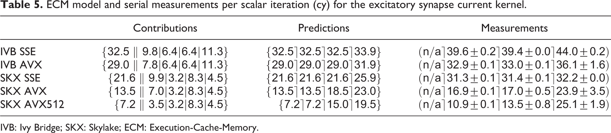
IVB: Ivy Bridge; SKX: Skylake; ECM: Execution-Cache-Memory.

The analysis reveals a complex situation. Both code versions on IVB and the SSE code on SKX are predicted to be core bound as long as the data fits into any cache. The AVX and AVX512 code on SKX, however, become data bound already in the L3 cache.

Again we used a benchmark data set containing only synapses to validate the model, with a size of roughly 80 kB and 500 kB for the L2 benchmarks and 1.5 MB and 11 MB for the L3 benchmark on the IVB and SKX architectures, respectively. On both CPUs, the model predictions are optimistic compared to measurements by a 10–50% margin. Interestingly, within each architecture, the model becomes more accurate as the SIMD width increases. Even though the predictions are not all within a small accuracy window, the model still allows us to correctly categorize the relevant bottlenecks and is especially effective in capturing the fact that on SKX with AVX512 the kernel is rather strongly data bound. Given the complex inter-dependencies between operations in the kernel, we speculate that a CP might be invalidating the full-throughput assumption of the ECM model, although this would not be sufficient to explain why the DRAM measurements are larger than the L2 and L3 measurements.

As a result from the analysis we conclude that, for an in-memory data set, the performance of the serial excitatory synapse current kernel would improve significantly only if in-core execution and data transfers were enhanced at the same time. Still the model predicts bandwidth saturation for all code variants, once run in parallel, at 4–6 cores.

3.3. Ion channels state kernels

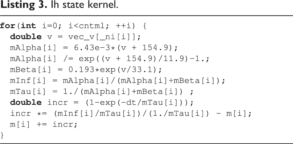
During the execution of a state kernel, the internal state variables of an instance of an ion channel or a synapse are integrated in time and advanced to the next timestep. Figure 2(a) shows that state kernels represent a significant portion of the overall runtime, although their relative importance is largest in the single-thread execution and decreases with shared-memory parallelism.

State kernels are characterized by a very large overlapping contribution $T_{OL}$ due to exponential functions and division operations, combined with low data requirements. This gives reason to expect a clearly core-bound situation. As an example, we show the code for the Ih state kernel in Listing 3. In analogy with the previous ion channel example, we treat the indices in _ni as contiguous. Therefore, this kernel requires reading one element each from one double and one integer array and writing one element each to three double arrays, amounting to a traffic of 60 B per iteration. On the other hand, the kernel needs three exponential function evaluations and eight divides, of which some might be eliminated by compiler optimizations (common subexpression elimination and substitution of multiple divides by the same denominator for a reciprocal and several multiplications).

Listing 3.

Ih state kernel.

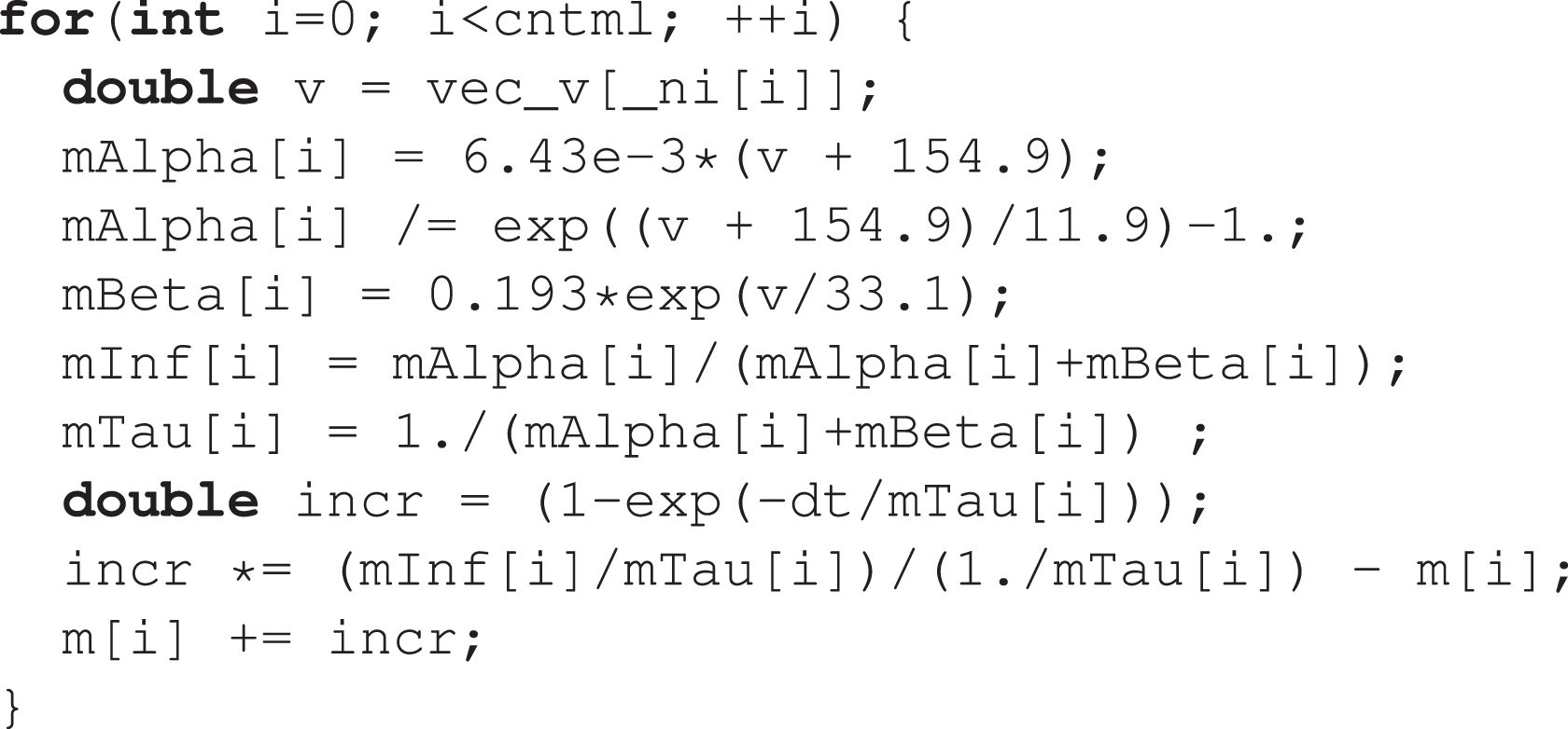
Again combining the IACA prediction with measured throughput data for exp() (see Table 2) and the data delay we arrive at the ECM predictions per scalar iteration in Table 6. State kernels can be considered as the polar opposite of current kernels in terms of their computational profile, and the model predicts that their performance will be independent of the location of the working set in the memory hierarchy. This also leads to the expectation that vectorization should yield massive improvements, but the ECM model says otherwise. According to the performance model these kernels are dominated by the throughput of the exp function and the eight divides, by comparable amounts; for instance, the SKX-AVX version spends 16 cy in divides and another 10.4 cy in exp(). No optimizations concerning the divides are done by the compiler, although the number of divides may be reduced to three by the methods mentioned above.

Table 6.

ECM model and serial measurements per scalar iteration (cy) for Ih state kernel.

	Contributions	Predictions	Measurements
IVB SSE	$\left\{90.5\parallel 4.5|2.9|2.9|5.1\right\}$	$\left\{90.5\text{⌉}90.5\text{⌉}90.5\text{⌉}90.5\right\}$	$\left(\text{n/a⌉}106.7\pm 0.1\text{⌉}106.5\pm 0.0\text{⌉}107.0\pm 0.0\right)$
IVB AVX	$\left\{80.0\parallel 4.5|2.9|2.9|5.1\right\}$	$\left\{80.0\text{⌉}80.0\text{⌉}80.0\text{⌉}80.0\right\}$	$\left(\text{n/a⌉}80.1\pm 0.1\text{⌉}80.0\pm 0.1\text{⌉}81.9\pm 0.1\right)$
SKX SSE	$\left\{36.1\parallel 6.0|1.4|3.2|2.0\right\}$	$\left\{36.1\text{⌉}36.1\text{⌉}36.1\text{⌉}36.1\right\}$	$\left(\text{n/a⌉}53.4\pm 0.2\text{⌉}53.4\pm 0.1\text{⌉}52.3\pm 0.0\right)$
SKX AVX	$\left\{26.4\parallel 3.4|1.4|3.2|2.0\right\}$	$\left\{26.4\text{⌉}26.4\text{⌉}26.4\text{⌉}26.4\right\}$	$\left(\text{n/a⌉}29.9\pm 0.1\text{⌉}29.9\pm 0.1\text{⌉}28.8\pm 0.0\right)$
SKX AVX512	$\left\{12.1\parallel 1.9|1.4|3.2|2.0\right\}$	$\left\{12.1\text{⌉}12.1\text{⌉}12.1\text{⌉}12.1\right\}$	$\left(\text{n/a⌉}18.6\pm 0.1\text{⌉}18.3\pm 0.1\text{⌉}19.0\pm 0.1\right)$

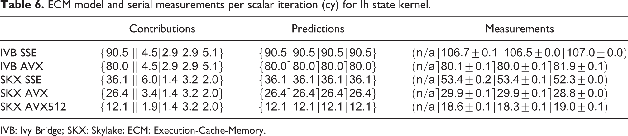
IVB: Ivy Bridge; SKX: Skylake; ECM: Execution-Cache-Memory.

Both architectures show only moderate speedup from SSE to AVX (13% on IVB and 37% on SKX, respectively). On IVB, this can be partly attributed to the mere 44% speedup for the exp() function (see Table 2), but the main cause on both CPUs is the constant throughput per divide operation, independent of the SIMD width. This is a well-known design tradeoff in Intel architectures: putting a large number of low-throughput units on a core does not pay off on a general-purpose CPU.

AVX512, on the other hand, exhibits a large speedup that cannot be explained by the above analysis. Inspection of the assembly code reveals that the compiler did not generate any divide instructions at all. Instead, it uses vrcp14d instructions together with Newton-Raphson steps for better throughput on SKX (see Intel (2018)).

We validated our predictions with data set sizes of 124 kB and 500 kB for the L2 benchmarks on IVB and SKX respectively, and a data set size of 5 MB for the L3 benchmarks on both architectures. Except for the AVX kernels, for which the accuracy is more than satisfying, the predictions are optimistic by between 15% and 35%. It must be stressed that when a loop is strongly core bound and has a long CP, the automatic out-of-order execution engine in the hardware may have a hard time overlapping successive loop iterations. Since the ECM model has no concept of this issue, predictions may be qualitative.

Despite all inaccuracies, the conclusion from the analysis is clear: Faster exponential functions, wider SIMD execution for divide instructions, and a higher clock frequency would immediately (and proportionally) boost the performance of the serial Ih state kernel. Memory bandwidth saturation is not expected on IVB, but on SKX the AVX and AVX512 versions will be able to hit the memory bandwidth limit, albeit at a larger number of cores than with the more data-bound kernels. Hence, boosting parallel performance is achieved by different means on the two chips.

3.4. Synaptic state kernels

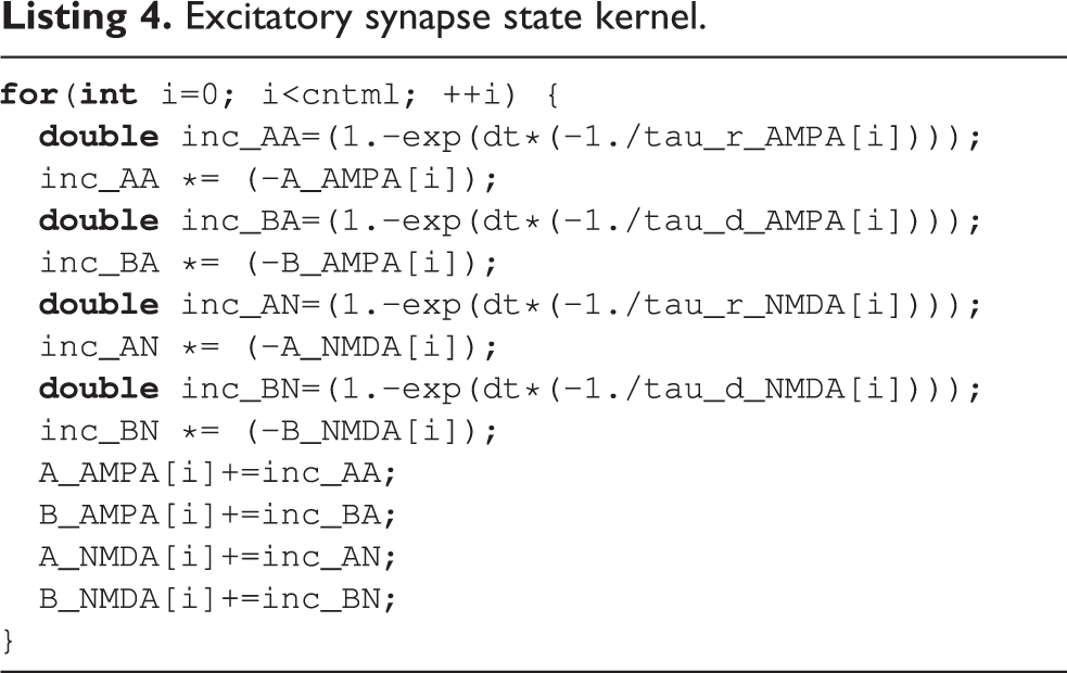
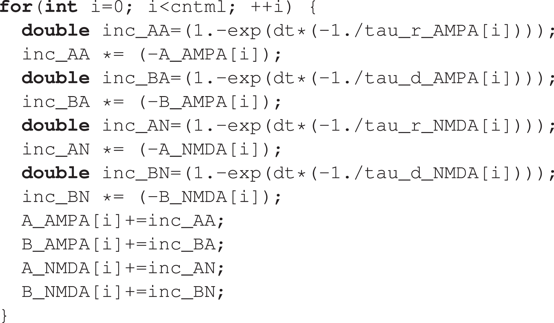
Synapse state kernels have computational properties similar to ion channel state kernels, that is, a dominating in-core overlapping contribution due to exponentials and divides, coupled with low data requirements. As an example, we show the code for the excitatory AMPA/NMDA synapse in Listing 4. This kernel reads one element each from four double arrays and updates one element each from four other double arrays, thus totaling 96 B of data volume per iteration. The ECM predictions per scalar iteration are listed in Table 7. An important observation to be made here is that using the AVX2 instruction set was crucial to obtaining good performance on Skylake-X. Indeed the exp function invoked by the AVX instruction set has a much worse throughput (despite having the same vector width) and thus would significantly degrade the performance of this kernel. As expected, all other observations and conclusions are the same as for the ion channel state kernels in the previous section. All predictions are optimistic by 20–30%.

Listing 4.

Excitatory synapse state kernel.

Table 7.

ECM model and serial measurements per scalar iteration (cy) for the excitatory synapse state kernel.

	Contributions	Predictions	Measurements
IVB SSE	$\left\{75.0\parallel 5.0|3.0|3.0|5.3\right\}$	$\left\{75.0\text{⌉}75.0\text{⌉}75.0\text{⌉}75.0\right\}$	$\left(\text{n/a⌉}93.0\pm 0.1\text{⌉}92.7\pm 0.0\text{⌉}94.3\pm 0.0\right)$
IVB AVX	$\left\{60.0\parallel 3.9|3.0|3.0|5.3\right\}$	$\left\{60.0\text{⌉}60.0\text{⌉}60.0\text{⌉}60.0\right\}$	$\left(\text{n/a⌉}75.0\pm 0.0\text{⌉}74.9\pm 0.0\text{⌉}75.0\pm 0.4\right)$
SKX SSE	$\left\{34.8\parallel 6.5|1.5|4.0|2.1\right\}$	$\left\{34.8\text{⌉}34.8\text{⌉}34.8\text{⌉}34.8\right\}$	$\left(\text{n/a⌉}45.7\pm 0.0\text{⌉}45.7\pm 0.0\text{⌉}44.9\pm 0.0\right)$
SKX AVX	$\left\{22.0\parallel 3.8|1.5|4.0|2.1\right\}$	$\left\{22.0\text{⌉}22.0\text{⌉}22.0\text{⌉}22.0\right\}$	$\left(\text{n/a⌉}25.5\pm 0.1\text{⌉}25.5\pm 0.1\text{⌉}25.7\pm 0.2\right)$
SKX AVX512	$\left\{9.7\parallel 1.7|1.5|4.0|2.1\right\}$	$\left\{9.7\text{⌉}9.7\text{⌉}9.7\text{⌉}9.7\right\}$	$\left(\text{n/a⌉}13.1\pm 0.1\text{⌉}13.4\pm 0.2\text{⌉}13.7\pm 0.2\right)$

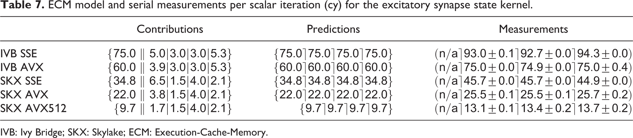
IVB: Ivy Bridge; SKX: Skylake; ECM: Execution-Cache-Memory.

3.5. Validation for all state and current kernels

To assess the validity of our performance and conclusions about bandwidth saturation on a real-world use case, we designed a representative data set based on the L5_TTPC1_cADpyr232_1 neuron, which can be downloaded from the Blue Brain NMC portal introduced in Ramaswamy et al. (2015). Since L5 pyramidal cells are among the cell types with the largest computational load in the reconstruction of the rat neocortex by Markram et al. (2015), this constitutes a highly representative subset of a full cortical column reconstruction. Commonly studied network arrangements are composed of a large number of neurons to be able to capture macroscopic effects, and even in the case of distributed simulations this usually amounts to a few hundred or even thousands of neurons per node. Given that the average detailed neuron among those in the Blue Brain NMC portal requires roughly 2 MB of data, this means that one can usually assume that data must be fetched from main memory each time. We used a sufficiently large data set consisting of 500 copies of the neuron mentioned above (for a total of 850 MB) as a building block for our benchmarks, eventually duplicating it according to the type of scaling scenario under analysis to avoid load imbalance issues.

Tables 8 and 9 show the predicted and measured runtimes of current and state kernels for the two architectures, all vectorization levels and serial versus full-socket parallel execution, while Figure 3 presents the performance scaling of these kernels across the cores of a chip. Interestingly, we observe a significant variability in serial runtime across kernels, with NaTs2_t state being the slowest because of its very high number of exponential and division operations. This phenomenon is particularly pronounced on IVB because of the large relative impact of vectorized divisions and exponentials compared to other vector operations. Overall, we observe a good match between the predicted and observed runtimes: barring a few exceptions our predictions always fall within 15% of the observations, and we are able to correctly capture the previously observed phenomenon that current kernels have a strongly saturating behavior, while state kernels need more cores to saturate or do not saturate at all (such as on IVB, and on SKX with SSE code). This corroborates our statements about optimization and codesign strategies: Boost in-core performance via reducing expensive operations (divides and exponentials), using wide SIMD cores and high clock speed for state, and look for a fast memory hierarchy to reduce the data delay of current kernels. As the runtime of state and current kernels decreases, we expect the relative importance of spike delivery and linear algebra to increase. We will cover these two kernels in Sections 3.6 and 3.7.

Figure 3.

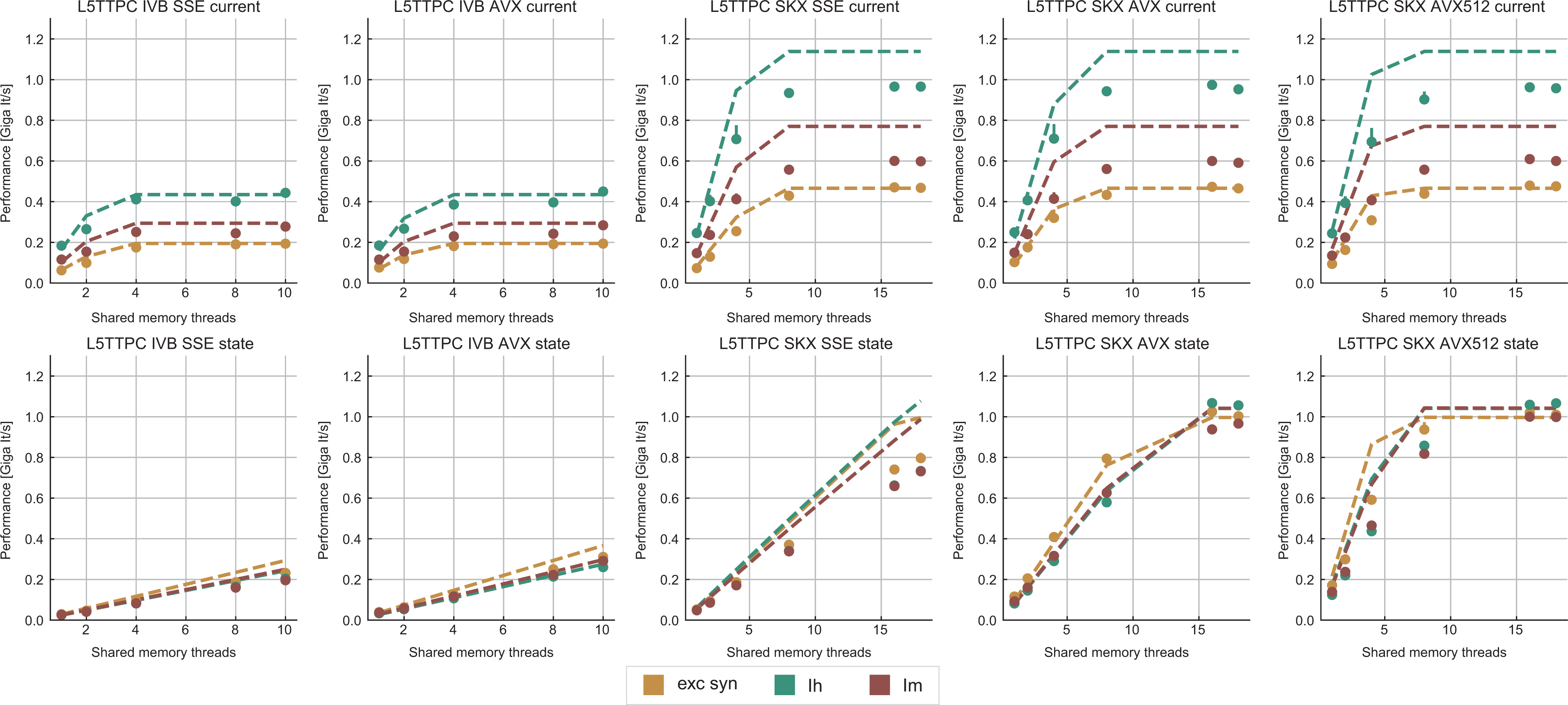
Performance predictions (dashed lines) and measurements (solid markers) for selected ion channel and state kernels, on all architectures and vectorization levels. The unit of measure for performance is Giga scalar iterations per wall clock second, denoted Giga It/s. Measurements points are computed as the median and error bars represent the 25- and 75-percentile out of 10 runs. Due to automatic clock frequency scaling, the performance predictions of each kernel were scaled by the kernel’s average clock frequency to preserve consistency with the measurements. Current kernels show a typical saturation behavior at low thread counts while state kernels either do not saturate at all (IVB), saturate at large thread counts (SKX-SSE, SKX-AVX) or saturate at moderate to low thread counts (SKX-AVX512). IVB: Ivy Bridge; SKX: Skylake.

Table 8.

Runtime for all current and state kernels on the IVB architecture (in-memory working set).^a

	SSE				AVX
	Serial		Full socket		Serial		Full socket
Kernel	Pred	Bench	Pred	Bench	Pred	Bench	Pred	Bench
exc syn current	33.9	35.2 $\pm$ 0.2	11.3	11.4 $\pm$ 0.0	31.9	28.9 $\pm$ 0.9	11.3	11.4 $\pm$ 0.1
inh syn current	28.3	26.5 $\pm$ 0.2	10.0	10.1 $\pm$ 0.1	27.3	26.4 $\pm$ 0.2	10.0	10.1 $\pm$ 0.1
NaTs2_t current	23.4	21.3 $\pm$ 0.2	8.1	8.4 $\pm$ 0.2	28.0	21.0 $\pm$ 0.2	8.1	8.2 $\pm$ 0.2
Ih current	13.3	12.0 $\pm$ 0.0	5.1	5.0 $\pm$ 0.1	13.8	11.9 $\pm$ 0.0	5.1	4.9 $\pm$ 0.1
Im current	21.5	19.0 $\pm$ 0.2	7.5	7.9 $\pm$ 0.1	21.6	19.0 $\pm$ 0.1	7.5	7.7 $\pm$ 0.1
SKv3_1 current	22.0	19.9 $\pm$ 0.1	7.7	7.9 $\pm$ 0.2	22.1	19.7 $\pm$ 0.1	7.7	7.7 $\pm$ 0.0
exc syn state	75.0	75.4 $\pm$ 0.0	7.5	9.5 $\pm$ 0.0	60.0	55.9 $\pm$ 0.0	6.0	7.1 $\pm$ 0.0
inh syn state	75.0	73.5 $\pm$ 0.1	7.5	9.3 $\pm$ 0.0	60.0	51.7 $\pm$ 0.0	6.0	6.5 $\pm$ 0.0
NaTs2_t state	220.5	162.7 $\pm$ 2.1	22.0	20.4 $\pm$ 0.0	196.0	142.5 $\pm$ 0.3	19.6	17.9 $\pm$ 0.0
Ih state	90.5	85.6 $\pm$ 0.0	9.1	10.8 $\pm$ 0.0	80.0	65.5 $\pm$ 0.0	8.0	8.4 $\pm$ 0.0
Im state	88.0	84.1 $\pm$ 0.2	8.8	11.2 $\pm$ 0.0	74.0	59.6 $\pm$ 0.6	7.4	7.6 $\pm$ 0.1
SKv3_1 state	83.5	79.8 $\pm$ 0.0	8.3	9.9 $\pm$ 0.0	73.0	60.7 $\pm$ 0.1	7.3	7.5 $\pm$ 0.0

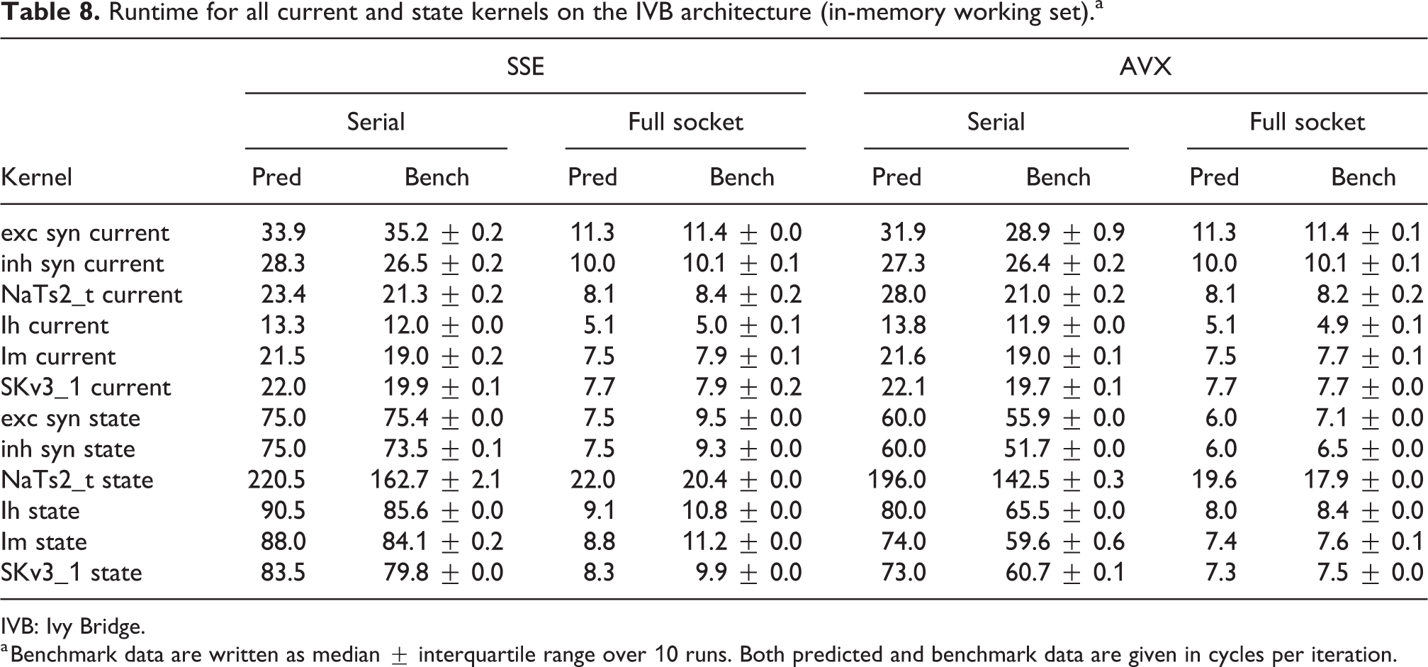
IVB: Ivy Bridge.

^a Benchmark data are written as median $\pm$ interquartile range over 10 runs. Both predicted and benchmark data are given in cycles per iteration.

Table 9.

Runtime for all current and state kernels on the SKX architecture (in-memory working set).^a

	SSE				AVX				AVX512
	Serial		Full socket		Serial		Full socket		Serial		Full socket
Kernel	Pred	Bench	Pred	Bench	Pred	Bench	Pred	Bench	Pred	Bench	Pred	Bench
exc syn current	25.9	28.6 $\pm$ 0.0	4.5	4.5 $\pm$ 0.1	23.0	20.4 $\pm$ 2.3	4.5	4.5 $\pm$ 0.1	19.5	22.3 $\pm$ 1.7	4.5	4.4 $\pm$ 0.1
inh syn current	21.6	22.5 $\pm$ 3.0	4.0	4.8 $\pm$ 0.0	19.8	22.5 $\pm$ 2.0	4.0	4.8 $\pm$ 0.1	16.6	23.4 $\pm$ 0.6	4.0	4.7 $\pm$ 0.1
NaTs2_t current	17.8	16.5 $\pm$ 1.1	3.2	4.1 $\pm$ 0.1	17.2	16.2 $\pm$ 1.1	3.2	4.0 $\pm$ 0.1	14.9	16.8 $\pm$ 0.7	3.2	4.0 $\pm$ 0.1
Ih current	9.7	9.3 $\pm$ 0.4	2.0	2.4 $\pm$ 0.1	10.5	9.2 $\pm$ 0.4	2.0	2.4 $\pm$ 0.1	9.0	9.4 $\pm$ 0.4	2.0	2.4 $\pm$ 0.0
Im current	16.1	15.6 $\pm$ 0.8	3.0	3.8 $\pm$ 0.1	15.4	15.3 $\pm$ 0.8	3.0	3.9 $\pm$ 0.1	13.6	17.0 $\pm$ 0.6	3.0	3.8 $\pm$ 0.1
SKv3_1 current	16.5	14.9 $\pm$ 0.7	3.1	3.8 $\pm$ 0.1	16.8	14.7 $\pm$ 0.8	3.1	3.9 $\pm$ 0.1	14.0	15.4 $\pm$ 0.4	3.1	3.8 $\pm$ 0.1
exc syn state	34.8	39.9 $\pm$ 0.0	2.1	2.6 $\pm$ 0.1	22.0	18.1 $\pm$ 0.1	2.1	2.1 $\pm$ 0.1	9.7	12.2 $\pm$ 0.2	2.1	2.1 $\pm$ 0.0
inh syn state	34.8	40.2 $\pm$ 0.0	2.1	2.6 $\pm$ 0.0	22.0	18.0 $\pm$ 0.0	2.1	2.1 $\pm$ 0.1	9.7	12.2 $\pm$ 0.3	2.1	2.1 $\pm$ 0.1
NaTs2_t state	86.7	94.5 $\pm$ 0.0	4.8	6.0 $\pm$ 0.0	64.5	51.1 $\pm$ 0.0	3.8	4.0 $\pm$ 0.1	25.3	29.0 $\pm$ 0.1	3.8	3.8 $\pm$ 0.1
Ih state	36.1	46.5 $\pm$ 0.0	2.0	3.0 $\pm$ 0.0	26.4	25.6 $\pm$ 0.0	2.0	2.0 $\pm$ 0.0	12.1	16.9 $\pm$ 0.1	2.0	2.0 $\pm$ 0.0
Im state	38.6	44.3 $\pm$ 0.1	2.1	2.9 $\pm$ 0.0	25.9	22.7 $\pm$ 0.1	2.0	2.2 $\pm$ 0.0	12.6	15.1 $\pm$ 0.3	2.0	2.1 $\pm$ 0.0
SKv3_1 state	34.0	40.8 $\pm$ 0.0	1.9	2.7 $\pm$ 0.0	24.5	21.7 $\pm$ 0.0	1.4	1.6 $\pm$ 0.0	16.1	13.3 $\pm$ 0.1	1.3	1.5 $\pm$ 0.0

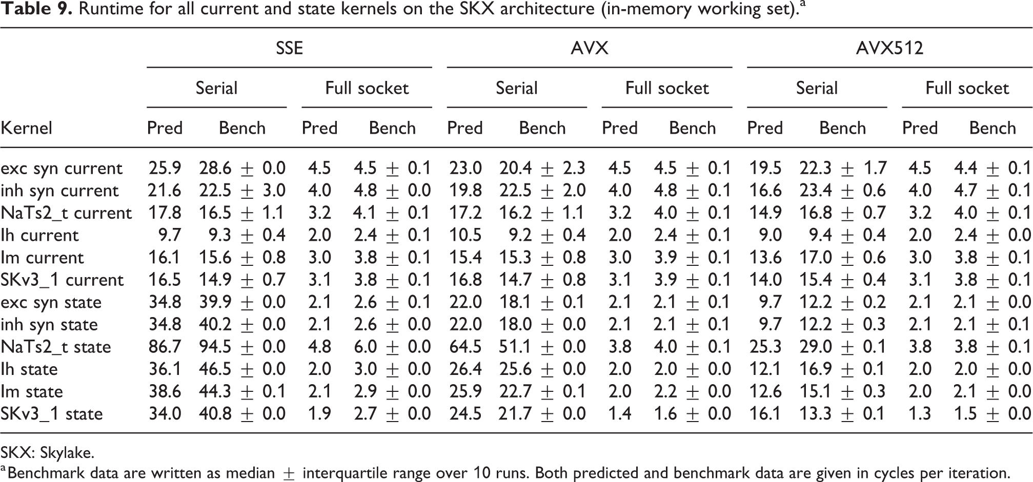
SKX: Skylake.

^a Benchmark data are written as median $\pm$ interquartile range over 10 runs. Both predicted and benchmark data are given in cycles per iteration.

In the rest of this section, we address some of the largest deviations between measurements and predictions by providing a tentative explanation for the failure of our performance model. As stated in the state kernel Sections 3.3 and 3.4, a long CP in the loop kernel code could be weakening the accuracy of our predictions due to a failure of the full throughput assumption. We believe that, in order to improve our predictions, a cycle-accurate simulation of the execution and in particular of the Out-of-Order (OoO) engine would be needed, thus invalidating our requirement for a simple analytical model. At large thread counts the predictions for current kernels are always within a reasonable error bound, while those for state kernels can be off by as much as 30%. The state kernels’ performance is often in a transitional phase between saturation and core-boundedness even at large thread counts, where the ECM model in the form we use it here is known to perform poorly as shown in Stengel et al. (2015). We do not plan to employ the adaptive latency penalty method as described in Hofmann et al. (2018) to correct for this discrepancy, because it is not only a modification of the machine model but also requires a parameter fit for every individual loop kernel. We believe that this is an undesirable trait in an analytic model.

3.6. Special kernels: Linear algebra

The most common approach for time integration of morphologically detailed neurons is to use an implicit method (typically backward-Euler or Crank-Nicolson) in order to take advantage of its stability properties for stiff problems. In Hines (1984), a linear-complexity algorithm based on Thomas (1949) was introduced to solve the quasi-tridiagonal system arising from the branched morphologies of neurons. This algorithm is based on a sparse representation of the matrix using three arrays of values (vec_a, vec_b, vec_d representing the upper, lower, and diagonal of the matrix, respectively) and one array of indices (parent_index). It is structured in two main phases: triangularization and a backward substitution. The code is shown in Listing 5. The boundary loop in the middle is executed but its trip count is so short in practice that we can ignore it in the analysis.

Listing 5.

Linear algebra kernel.

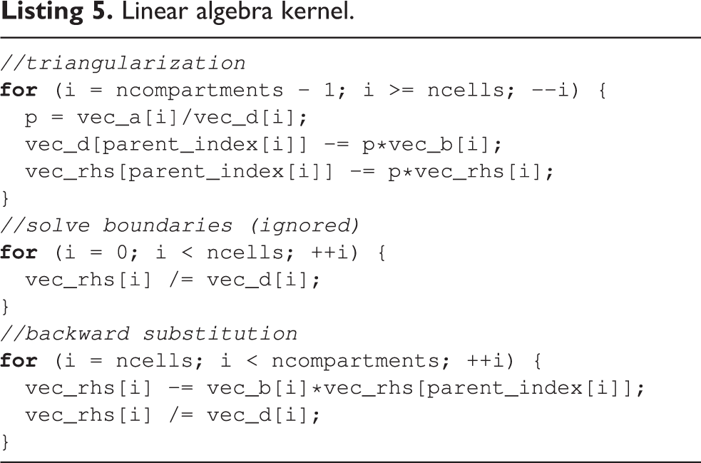
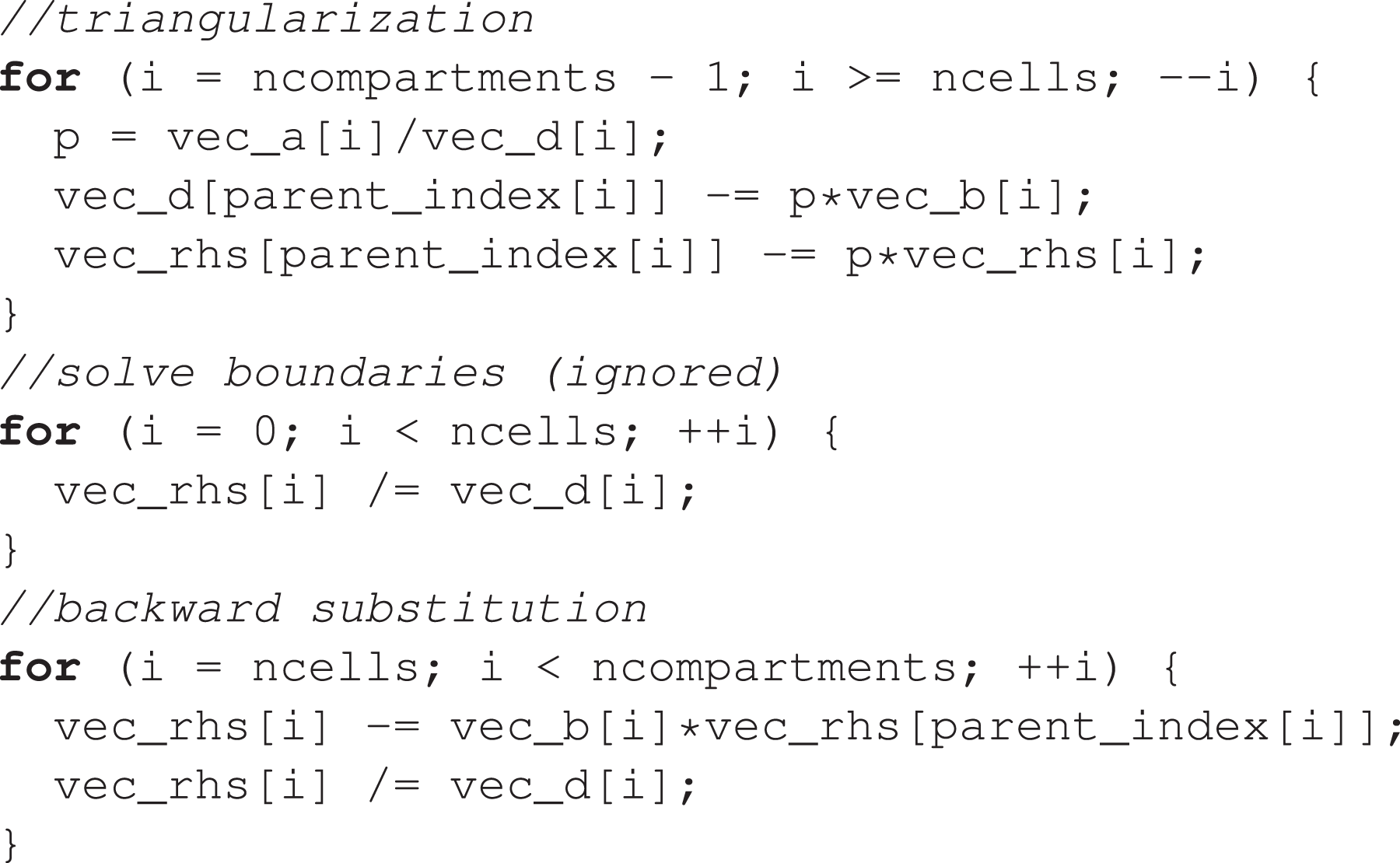
To construct a performance model for this kernel, we must tackle a few challenges: Indirect accesses make it difficult to estimate the data traffic, and dependencies between loop iterations could break the full-throughput hypothesis. Moreover, a yet-unpublished optimized variant of the algorithm proposed in Hines (1984) that exploits a permutation of node indices to maximize data locality is executed by default by the simulation engine. ³ For reasons of brevity of exposition, we restrict our analysis to this optimized variant of the solver. Additionally, we will ignore the solve boundaries loop in our analysis because its impact on the overall performance is always neglectable, for two reasons: the number of cells is always much smaller than the number of compartments so this loop makes very few iterations compared to the others, and there are no data dependencies so this loop can be trivially vectorized.

In order to give a runtime estimate, we examine two corner-case scenarios. The first, optimistic scenario assumes that indirect accesses can exploit spatial data locality in caches and thus do not generate any additional memory traffic. The combined data traffic requirements of triangularization and back-substitution then amount to reading one element each from four double arrays and two integer arrays, and writing one element each to three double arrays, that is, 88 B per iteration. Considering the opposite extreme, it might happen that at every branching point the value of parent_index[i] is so much smaller than i that this generates an additional cache line of data traffic through the full memory hierarchy. We call this the worst-case branching hypothesis, in which we adjust the memory traffic predictions by assuming that every section boundary, that is, the location of a potential discontinuity in the parent_index array, requires a full cache line transfer of which only one variable will constitute useful data.

Even though the dependencies between loop iterations could potentially break the full-throughput hypothesis, considering that compartment indices are by default internally rearranged to optimize data locality we still use the full throughput as a basis for our predictions. It should be noted that indirect addressing and potential loop dependencies hinder vectorization. IACA reports that the combined inverse throughput of triangularization and back substitution amounts to 28 cy/it for IVB and 8.12 cy/it for SKX, while $T_{nOL}=6$ cy/it for both architectures. This leads to the runtime predictions in Table 10.

Table 10.

ECM model and serial measurements per scalar iteration (cy) for the linear algebra kernel.^a

	Contributions	$T_{ECM}^{Mem}$	Measured
IVB	$\left\{28.0\parallel 6.0|2.8|2.8|4.8\right\}$	28.0	$32.6\pm 4.4$
SKX	$\left\{8.1\parallel 6.0|1.4|4.0|1.9\right\}$	13.3	$18.8\pm 5.3$

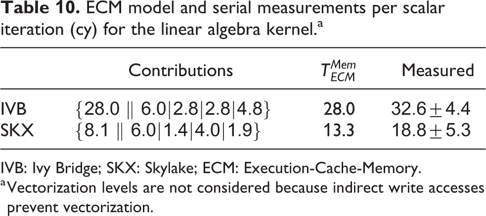
IVB: Ivy Bridge; SKX: Skylake; ECM: Execution-Cache-Memory.

^a Vectorization levels are not considered because indirect write accesses prevent vectorization.

We measured the performance of the linear algebra kernel on a specially designed data set with 15 K neurons and neither ion channels nor synapses. Since the memory requirement of this kernel is only of 36 B per compartment, the number of neurons can have an important effect on performance as the data set for even a few hundred neurons could easily fit in a cache. This would lead to data reuse that, while beneficial to performance, would invalidate our model. Thus the number of neurons was chosen large enough to ensure that the only data locality effects are intrinsic to the algorithm and not a consequence of a small data set. Our predictions based on the full-throughput hypothesis are validated by measurements of both the performance (see Figure 4) and the memory traffic (last row in Table 11). This kernel highlights very strongly an important difference between the two architectures: SKX has a much better divide unit, which is able to deliver one result every four cycles, whereas IVB’s divider needs 14. This ratio is almost exactly reflected in the $T_{OL}$ prediction, although the triangularization kernel on SKX is actually load bound by a small margin. This large difference in $T_{OL}$ causes different single-core bottlenecks: While the execution on IVB clearly core bound, it is strongly data bound on SKX. The single-core medians are a little higher than predicted but also prone to some statistical variation; the best measured value is very close to the model. Saturation is predicted at six cores on IVB and seven cores on SKX. Starting from the newer architecture, the only way to boost performance would be to enhance the performance of the memory hierarchy (in serial mode) or the memory bandwidth (in parallel). Having more than ten cores per chip would be a waste of transistors.

Figure 4.

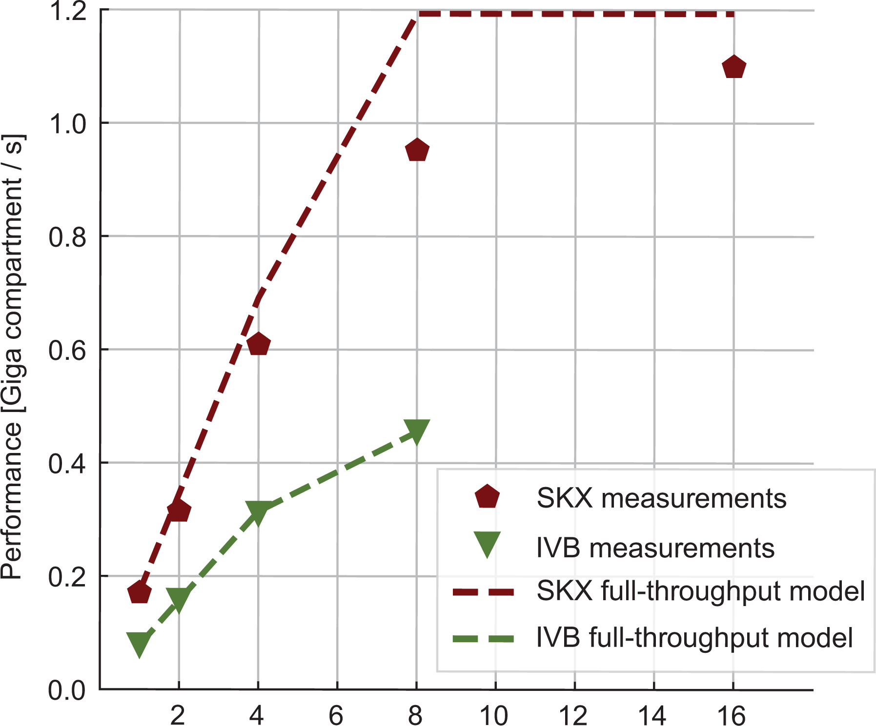
Measured performance (markers) and predictions (lines) for the linear algebra kernel in Giga-compartments per second. Dashed lines represent the model predictions in the optimistic full-throughput scenario.

Table 11.

Predicted (pred) and measured (meas) data volume per iteration from main memory.^a

Kernel	Pred (B)	IVB meas (B)	SKX meas (B)
exc syn current	205.3	205.2 $\pm$ 2.8	207.1 $\pm$ 2.1
inh syn current	181.3	183.3 $\pm$ 5.2	204.0 $\pm$ 8.4
NaTs2_t current	148.0	144.3 $\pm$ 8.2	139.4 $\pm$ 11.0
Ih current	92.0	79.2 $\pm$ 4.3	80.2 $\pm$ 9.2
Im current	136.0	128.9 $\pm$ 5.8	133.4 $\pm$ 10.8
SKv3_1 current	140.0	128.8 $\pm$ 8.0	128.1 $\pm$ 13.3
exc syn state	96.0	95.6 $\pm$ 1.9	94.3 $\pm$ 1.3
inh syn state	96.0	91.3 $\pm$ 5.3	88.6 $\pm$ 4.6
NaTs2_t state	172.0	197.4 $\pm$ 1.9	166.2 $\pm$ 2.2
Ih state	92.0	88.0 $\pm$ 0.3	87.7 $\pm$ 1.2
Im state	92.0	118.0 $\pm$ 5.8	89.1 $\pm$ 2.0
SKv3_1 state	60.0	92.5 $\pm$ 8.3	56.6 $\pm$ 2.1
Linear algebra	88.0	90.6 $\pm$ 7.6	90.7 $\pm$ 4.2

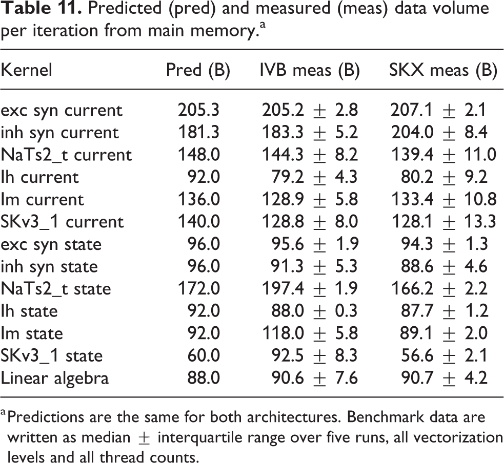
^a Predictions are the same for both architectures. Benchmark data are written as median $\pm$ interquartile range over five runs, all vectorization levels and all thread counts.

We remark that it remains unclear whether the node permutation optimization is applicable in all cases or suffers from some constraints, and that our full-throughput predictions heavily rely on it. Therefore it may happen that, in some cases where it is impossible to reorder the nodes effectively, our predictions would only provide an optimistic upper bound on performance.

3.7. Special kernels: Spike delivery

Accounting for network connectivity and event-driven spike exchange between neurons is, in terms of algorithm design, the most distinguishing feature of neural tissue simulations. In terms of performance, however, spike delivery plays a marginal role in the simulation of morphologically detailed neurons, rarely exceeding 10% of the total runtime (see Figure 2(a)).

The source code for the spike delivery kernel of AMPA/NMDA excitatory synapses is shown in Listing 6. For benchmarking purposes, we executed this kernel as the body of a loop iterating over a vector of spike events, which was previously populated by popping a priority queue. ⁴ This only represents a small deviation from the original implementation in CoreNEURON, where the kernel is directly called at every pop of the priority queue. However, it was necessary to implement this in order to separate the performance of the kernels from the performance of the queue operations.

Listing 6.

Event-driven spike delivery kernel.

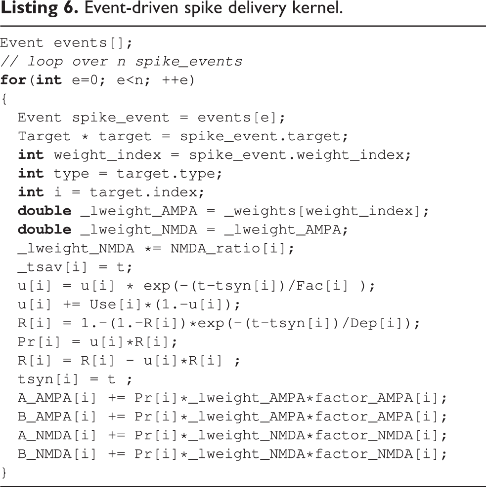
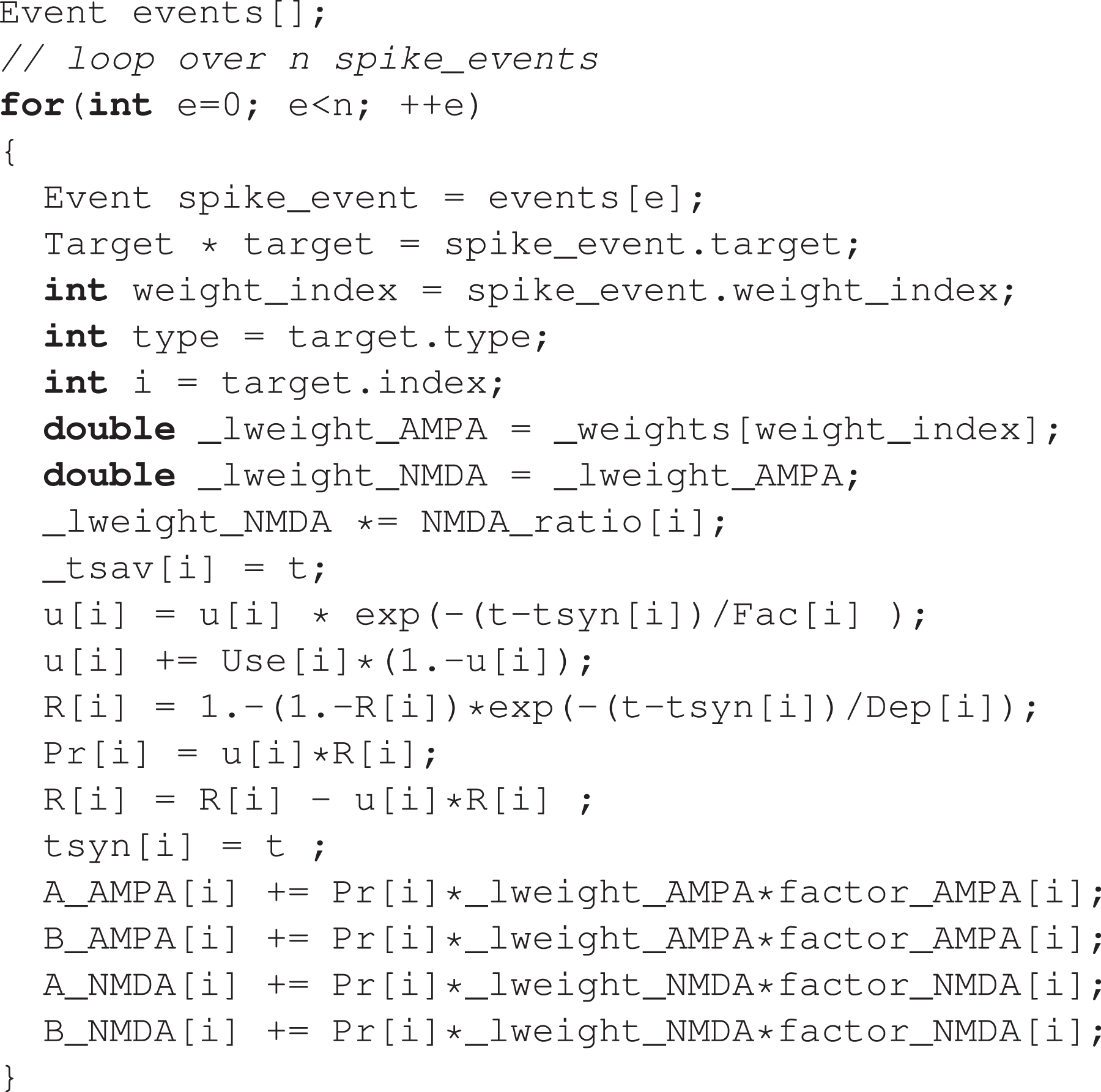
This kernel is characterized by erratic memory accesses indexed by i, as well as several compute-intensive operations such as divisions and exponentials, thus making it challenging to model. In terms of memory traffic we consider two scenarios: a best-case one in which all synapses are activated in memory-contiguous order and a worst-case scenario in which synapses are activated in random order. Note that the former represents a hypothetical situation which is highly unlikely in real-world simulations, while the latter is probably much more realistic. In the best-case scenario, we assume the execution engine will be able to fully pipeline the execution and hide all latencies. Thus we base our performance predictions on either the full-throughput hypothesis or a CP. Given the complex chain of interdependencies in the kernel, we suspect that a CP effect could also be present. For the IVB architecture, we can directly use IACA with the -analysis LATENCY option, while for SKX, we resorted to using the estimate for the Haswell architecture (HSW) from IACA v2.1, because latency analysis is no longer supported in IACA v3.0. The CP values are also reported in Table 12. Given that this kernel requires a read-only transfer on seven double arrays, three integer arrays and one pointer array, and an update or write/write-allocate transfer on nine double arrays, we estimate a (best-case) memory traffic of 220 B per iteration. From IACA, we learn that the inverse throughput of this kernel is 29.5 cy/it on IVB and 27.6 cy/it on SKX, while $T_{nOL}$ is 19.5 cy/it on both architectures, and as with the linear algebra kernel the indirect accesses prevent vectorization. Under the full-throughput assumption, this leads to the single-thread predictions per iteration shown in Table 13.

Table 12.

ECM model per scalar iteration (cy) for the spike delivery kernel.^a

	Contributions	$T_{ECM}^{Mem}$	CP
IVB	$\left\{85.1\parallel 19.5|6.9|6.9|12.1\right\}$	85.1	207.0
SKX	$\left\{57.8\parallel 19.5|3.4|9.2|4.8\right\}$	57.8	123.4

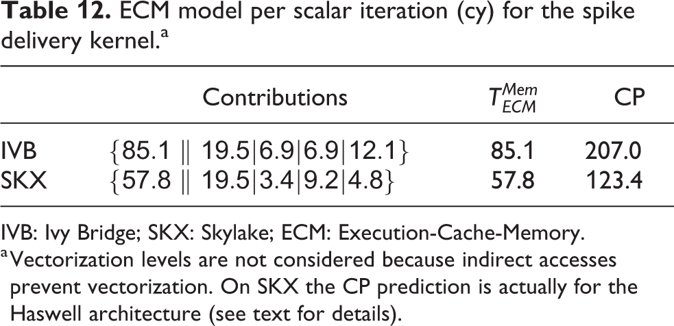
IVB: Ivy Bridge; SKX: Skylake; ECM: Execution-Cache-Memory.

^a Vectorization levels are not considered because indirect accesses prevent vectorization. On SKX the CP prediction is actually for the Haswell architecture (see text for details).

Table 13.

Spike delivery runtime predictions and median measurements ( $\pm$ interquartile range) under the best-case (BC) and worst-case (WC) scenarios, in serial (S) and parallel (P) execution.^a

	Runtime IVB (cy)		Runtime SKX (cy)
(lr)2–3 (lr)4–5	Pred	Meas	Pred	Meas
BC-S	207.0	$183.9\pm 0.5$	123.4	$122.1\pm 0.5$
WC-S	540.0	$1064.8\pm 55.6$	540.0	$740.0\pm 2.1$
BC-P	25.9	$23.1\pm 0.0$	7.7	$7.9\pm 0.1$
WC-P	96.8	$161.7\pm 11.3$	45.0	$58.8\pm 0.1$

IVB: Ivy Bridge; SKX: Skylake.

^a In the case of parallel execution, we report the values for 8 threads on IVB and 16 threads on SKX.

In the worst-case scenario, we assume that a full cache line of data needs to be brought in from memory for every data access. Assuming that the variables spike_event.target and spike_event.weight_index can still be read contiguously, the kernel requires 27 noncontiguous data accesses plus reading from one pointer and one integer array, which amounts to a predicted memory traffic of 1740 B per iteration. Estimating the runtime is more complex: On the one hand, it seems clear that the memory requests to arbitrary locations should have an effect on performance. On the other hand, this kernel does not have the typical latency-bound structure in which an iteration requires the full completion of the previous one before being executed, because the indirect accesses of one iteration do not depend on the completion of any operation from the previous iteration. Consequently, target indices can be made available via prefetching in the target.index variable, enabling the hardware to schedule indirect loads in advance. Indeed, multiplying the number of memory accesses by the memory latency leads to a prediction that is more than ten times too pessimistic. Instead, we created a synthetic stream-copy benchmark with a similar number of memory accesses and the same access pattern and determined the average latency per memory access to be around $20.1\pm 1.3$ cycles for both architectures. To obtain a runtime prediction for the serial execution, we then multiply this average latency by the number of memory accesses, yielding a prediction of 540 cy/it. To extend this to the multi-threaded case, we assume that either the bandwidth is saturated (and thus our performance prediction corresponds to the Roofline model) or the performance scales linearly with the number of threads. The consequences of a kernel being data bound or compute bound and how optimistic vs. pessimistic predictions can come about are summarized in Table 14.

Table 14.

Possible causes for degradation of accuracy in ECM model.

Prediction is…	Data-bound kernel	Core-bound kernel
Optimistic	Memory latency	CP
Pessimistic	Data locality	OoO engine

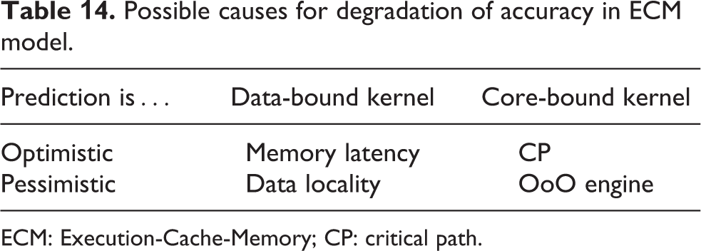
ECM: Execution-Cache-Memory; CP: critical path.

For validation, we designed a benchmark data set with 16 neurons and $4\times {10}^5$ synapses per neuron. In the best-case scenario, we artificially activate all synapses in order of instantiation, while for the worst-case scenario, we activate all synapses using random input events, trying to ensure that synapses close to each other in memory would not be activated at similar times. Neglecting network effects that could come from small networks with lower-than-physiological level of activity, our benchmark should be close to reality as long as the data set of synapses fits only in main memory. The validation results are shown in Figure 5 and Table 13. In the serial best-case scenario the measured runtime is so close to the CP-assumption that we can safely discard the full-throughput hypothesis and assume that under ideal memory access conditions this kernel is bounded by the dependencies within one loop iteration. In the worst-case scenario, while the data volume predictions are quite correct, the runtime predictions are off by factors from 50% up to 100% (see also Table 13). A reason for this could be that a CP estimate should be added to the memory access latency. Unfortunately, this does not give a sufficiently convincing improvement in the estimates: On IVB, IACA computes a CP of 79 cy/it to which we should add twice the latency of a scalar exponential, benchmarked to be around 64 cy. This leads to an adjusted prediction of 747 cy/it, which is still far from the measured 1087 cy/it. Considering that only a strikingly correct prediction would justify an adjustment to our model, we prefer to keep the old but simpler estimate. One should add that the worst-case scenario is beyond the applicability of the ECM model, so our analysis stretches the model very far.

Figure 5.

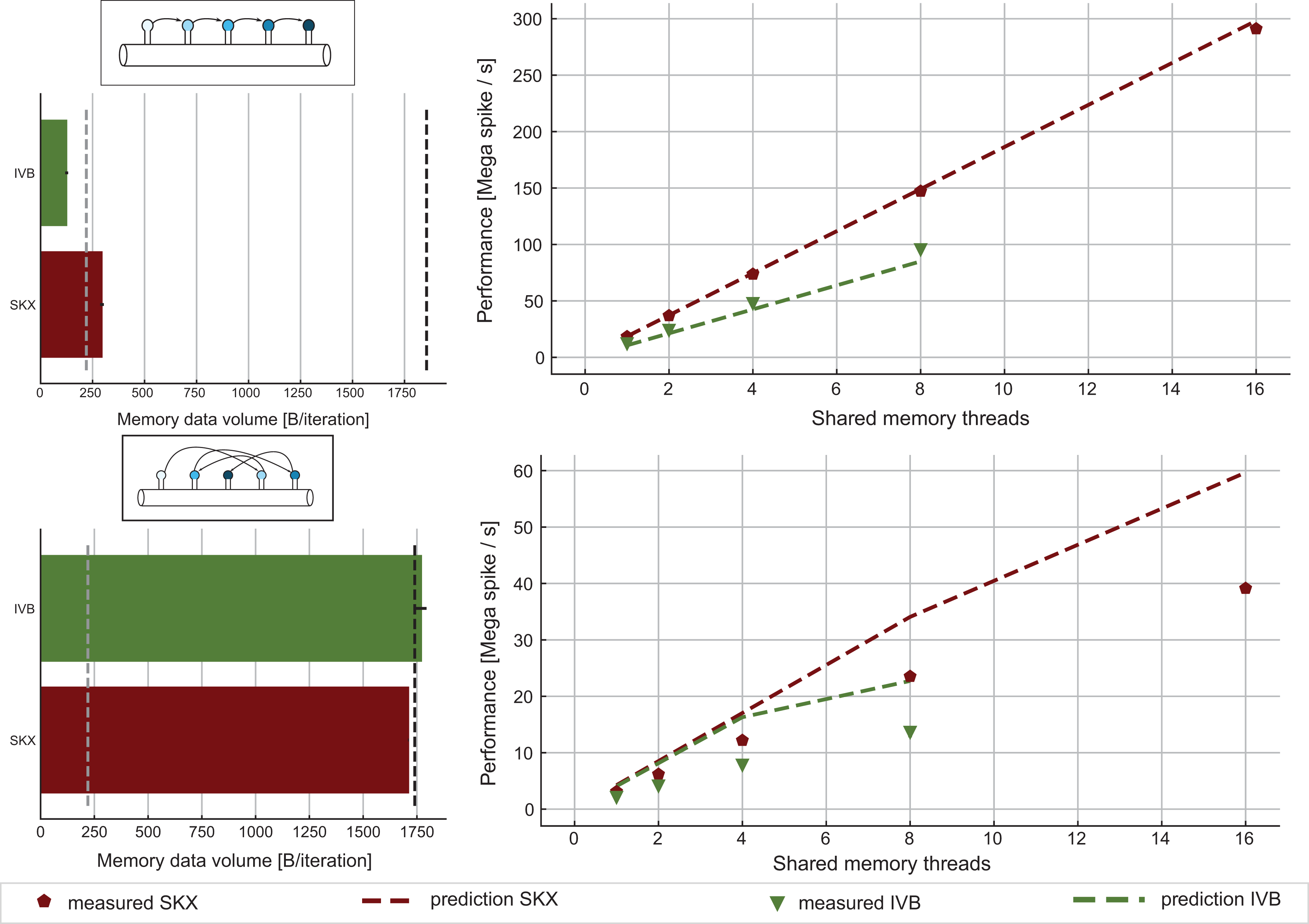
ECM model and measurements for the spike delivery kernel. Top: Best-case scenario where synapses are activated in contiguous memory order. In this case, there is no excess data traffic as shown by the bar plot on the left. The performance predictions on the right (dashed lines) are made by assuming that the kernel’s runtime is equal to its CP as predicted by IACA. Measurements (solid markers) substantiate this hypothesis. Bottom: Worst-case scenario where synapses are activated in random order. This scenario corresponds to the typical use-case. We assume that for every array access a full cache line of data traffic is generated, but only one element of the array is relevant. ECM: Execution-Cache-Memory; IACA: Intel Architecture Code Analyzer; CP: critical path.

4. Discussion

Using the ECM performance model, we have analyzed the performance profile of the simulation algorithm of morphologically detailed neurons as implemented in the CoreNEURON package. Within its design space, the ECM model yielded accurate predictions for the runtime of 13 kernels on real-world data sets. It must be stressed that some of these kernels are rather intricate, with hundreds of machine instructions and many parallel data streams. This confirms that analytic modeling is good for more than simple, educational benchmark cases. We have also, for the first time, set up the ECM model for the Intel Skylake-X architecture, whose cache hierarchy differs considerably from earlier Intel server CPUs. Our analysis shows that the non-overlapping assumption applies there as well, including all data paths between main memory, the L2 cache and the victim L3. Note that a reproducibility appendix is available at Cremonesi et al. (2019).

As expected, the modeling error was larger in situations where the bottleneck was neither streaming data access nor in-core instruction throughput. By making a few simplifying assumptions we were still able to predict with good accuracy the performance of a kernel with a complex memory access pattern and dependencies between loop iterations such as the tridiagonal Hines solver Hines (1984).

On the other hand, if the bottleneck is the memory latency, which is the case with the spike delivery kernel, the ECM model could only provide upper and lower bounds. In this case where the deviation from the measurement was especially large, we could at least pinpoint possible causes for the failure. It is left to future work on the foundations of the ECM model to extend its validity in those settings.

In conclusion, the ECM model was always able to correctly identify the computational characteristics and thus the bottlenecks of the 14 kernels under investigation, thus providing valuable insight to the performance-aware developers and modelers. In the following we use these crucial insights to give clear guidelines for both the optimization of simulation code and the codesign of an “ideal” processor architecture for neuron simulations. Given that memory locality plays a crucial role in our analysis, we structure our discussion based on the size of the biological network being simulated, that is, the total number of neurons in the data set. We mostly concentrate on the Skylake-X architecture since it is the most recent one, and no ECM model was published for it to date. Where relevant, we compare to the Ivy Bridge architecture to show the benefit of hardware improvements over three generations of Intel server processors.

4.1. Small networks (in cache)

4.1.1. Serial performance properties of small networks

One of the main insights offered by the ECM model is the possibility to identify and quantify the performance bottleneck of each kernel. In the simulation of morphologically detailed neurons, we found that ion channel current kernels are data bound while all state kernels are core bound for all cache levels, all SIMD levels and both architectures considered. The case of excitatory synapse current kernel was special in that on both SKX and IVB, the kernel was core bound as long as the data set fits in the caches, but switched to data-bound when the data comes from memory. This effect was most prominent on SKX-AVX512. In the extreme strong scaling scenario where data fits in the cache, this points to two optimizations: optimize expensive operations such as div and exp for all state kernels and the excitatory synapse current kernel, and minimize data movement for the ion channel current kernels. In terms of codesign, high-frequency cores with high-throughput instructions are ideal for all state kernels while fast data-paths within the cache hierarchy would optimize ion channel current kernels.

4.1.2. SIMD parallelism and small networks

The possibility to execute high-throughput SIMD vector instructions can potentially provide great returns in terms of speedup at a low hardware and programming cost. In this analysis, we observed that wider SIMD units were indeed capable of providing benefits in terms of reduced runtime, but we also failed to observe the ideal speedup factor. Moreover, Skylake-X showed diminishing returns as the SIMD units grew wider. Applying the ECM model to the scenario where data comes from cache, we discovered that all state kernels show significant speedups from vectorization and would benefit even more from even wider SIMD units. The synapse current kernels benefit from SIMD instructions at least for data in the L1 or L2 cache. Ion channel current kernels show only small speedups from vectorization because their performance is solely determined by the speed of the data transfer, even when the working set fits into a cache.

The importance of high-throughput exp and div functions cannot be overrated, which is punctuated by the large performance gain from Ivy Bridge to Skylake-X for kernels where these functions contribute significantly to the runtime. We have observed that the compiler was sometimes not able to eliminate expensive divide operations, although this was possible and allowed by the optimization flags.

4.2. Large networks (out of cache)

4.2.1. Memory bandwidth saturation of large networks

At constant memory bandwidth, a sufficient number of cores and/or high enough clock speed will render almost every code memory bound. One of the key insights delivered by the ECM model is how many cores are required to achieve saturation of the memory bandwidth during shared-memory execution, and what factors this number depends on. We applied saturation analysis to the full simulation loop by predicting the memory bandwidth of each kernel for different numbers of cores and compared it to the ratio of measured memory bandwidth to theoretical maximum bandwidth, weighted by the runtime of each kernel. Figure 6 shows the results, highlighting the remarkable power of the AVX512 technology on SKX, which is able to almost fully saturate the memory bandwidth using only seven cores. Since in-core features come essentially for free but more cores are more expensive, this means that in the max-filling scenario where the number of neurons being simulated is large and the data fits in main memory, the most cost-effective hardware platform for this code among the architectures considered is one with AVX512 support, high clock speed and a moderate core count. To further quantify the tradeoff between clock speed and saturation on SKX-AVX512, we computed the saturation point, which we define as the number of threads required to utilize at least 90% of the theoretical memory bandwidth, at different clock frequencies for the SKX architecture (assuming no clock frequency reduction). The results in Table 15 highlight once again that, as long as the working set is in main memory, vectorization pushes the bottleneck towards the memory bandwidth in the shared-memory execution. We have to allow some room for error in the measurements of the memory bandwidth and the over-optimistic ECM model near the saturation point as shown in Stengel et al. (2015), but the model indicates clearly that cores can be traded for clock speed, which provides a convenient price-performance optimization space.

Figure 6.

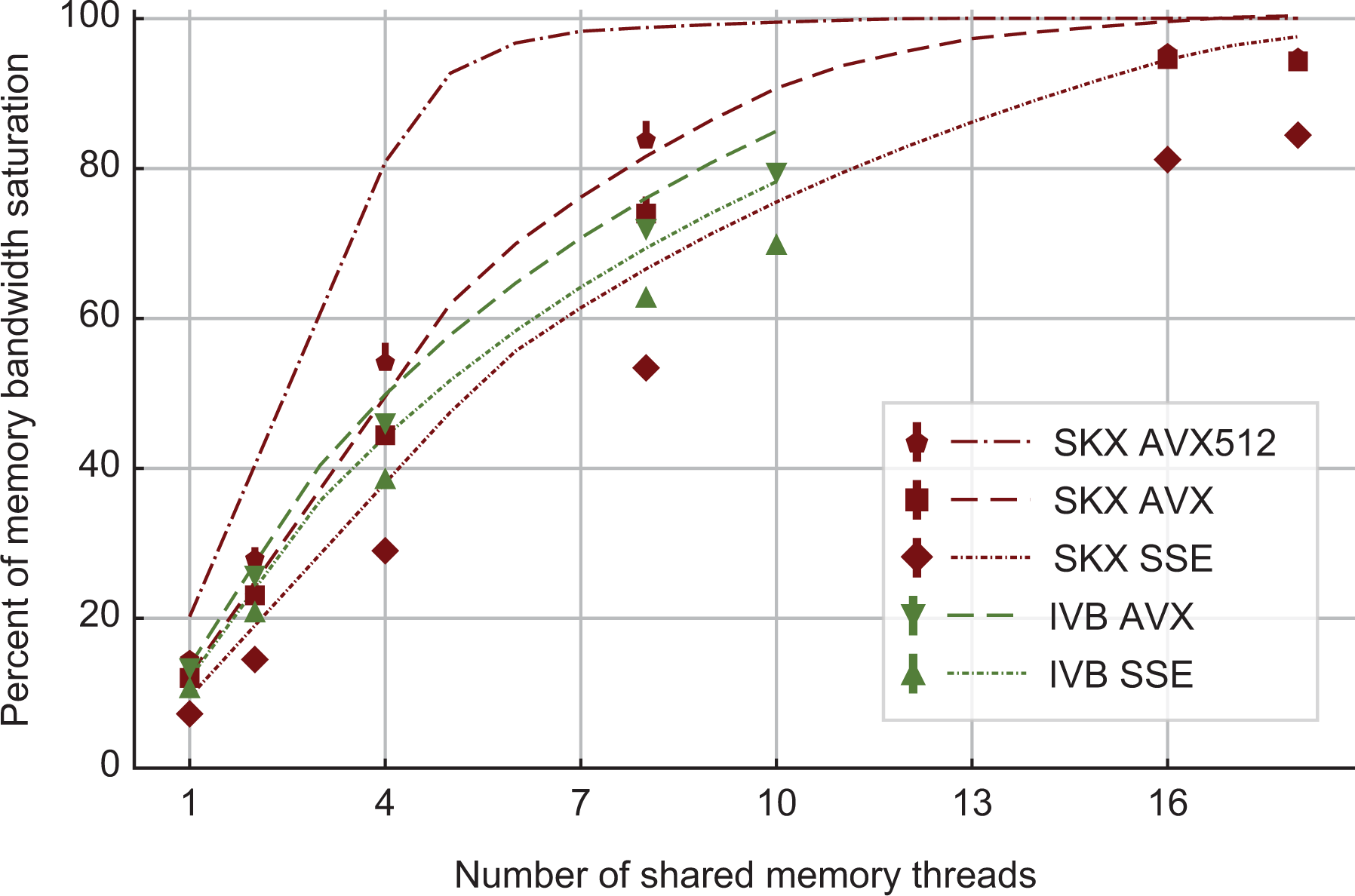
Predicted and measured memory bandwidth utilization, as a fraction of the maximum memory bandwidth. Dashed lines are obtained by predicting the average memory bandwidth of the full application while solid markers represent bandwidth measurements by LIKWID. Due to automatic clock frequency scaling, the maximum memory bandwidth was rescaled by the ratio of average clock frequency to nominal clock frequency. On SKX, AVX512 code can saturate the memory bandwidth of the socket at less than half the total number of cores even at the base clock frequency. SKX: Skylake.

Table 15.

Saturation point as predicted by the ECM model as a function of clock frequency.^a

	CPU @ 2.3 GHz	CPU @ 3.5 GHz
SKX SSE	16	11
SKX AVX	12	8
SKX AVX512	6	4

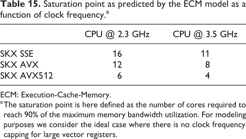
ECM: Execution-Cache-Memory.

^a The saturation point is here defined as the number of cores required to reach 90% of the maximum memory bandwidth utilization. For modeling purposes we consider the ideal case where there is no clock frequency capping for large vector registers.

4.2.2. Wide SIMD and large networks

For in-memory data sets, wide SIMD execution helps to push the saturation point to a smaller number of cores, as shown in Table 15 and Figure 6, but it will certainly not increase the saturated performance. Hypothetical hardware with even wider SIMD units would thus have to be supported by a larger memory bandwidth to be fully effective. Moreover, as clearly shown by the ECM model analysis, wider SIMD execution would ultimately make even the state kernels data bound. In the mid-term future it would hence be advisable to put more emphasis on fast clock speeds and better memory bandwidth than on pushing towards wider SIMD units, at least for the workloads discussed in this work.

When choosing the most fitting cluster architecture one is thus left with the decision between a larger number of high-frequency chips with moderate memory bandwidth and a smaller amount of lower-frequency chips with large memory bandwidth and more cores. Roughly speaking, larger bandwidth is more expensive than faster clock speed, but the decision has to be made according to the market and pricing situation at hand, which unfortunately tends to be rather volatile.

4.2.3. Memory hierarchy for large networks

There is practically no temporal locality in the data access patterns of almost all kernels. This means that cache size is insignificant for determining the performance of large networks of detailed neuron simulations. Unfortunately, cache size is not a hardware parameter that one is free to choose when procuring clusters of off-the-shelf CPUs. Moreover, using the decomposition of the runtime by the ECM model, we observe that contributions from different levels of the memory hierarchy are rather evenly distributed. Hence, the runtime of data-bound kernels could best be improved by reducing the data volume. A common programming technique to solve this problem is loop fusion, by which two or more back-to-back kernels that read or write some common data structures are cast into a single loop in order to leverage temporal locality and thus increase the arithmetic intensity. The structure of the NEURON code does not easily allow this.

5. Conclusions

In this work, we have demonstrated the applicability of the ECM analytic performance model to analyze and predict the bottlenecks and runtime of simulations of biological neural networks. The need for such modeling is demonstrated by the ongoing development efforts to optimize simulation code for current state of the art HPC platforms, coupled with demands for simulators able to handle faster and larger data sets on present and future architectures. Using the performance model we identified high-frequency cores capable of high-throughput div and exp operations and wide cache data paths as the most desirable features for real-time simulations of small neuron networks, while high memory bandwidth, few cores with moderate to high SIMD parallelism and a shallow memory hierarchy are the ideal hardware characteristics for simulations of large networks. We have not discussed the implications of such design choices in terms of power dissipation and energy consumption, which is clearly beyond the scope of this work. However, our results show that if standard off-the-shelf processors must be used, the strongly data-bound characteristics of simulations of larger networks allow for significant energy savings when the full parameter range of number of cores and clock speed is exploited. This is because the memory bandwidth of modern CPUs is rather insensitive to their clock frequency; reducing the clock speed thus has a minor impact on the time to solution of a code if the code stays memory bound. Since the power dissipation of a CPU depends rather strongly on the frequency, this is a major energy saving strategy. Further savings are possible if one allows to compromise time to solution. In that case, that is, when the code performance scales across the cores, an optimal frequency for minimal energy to solution can be found. These insights have recently been obtained using analytic modeling and measurements. Details can be found in Hager et al. (2013), De Vogeleer et al. (2014), and Hofmann et al. (2018). As for special-purpose hardware designs, the demonstrated insignificance of cache sizes would call for strongly compute-centric architectures, in which the cache can be kept small and its contribution to power dissipation thus be greatly reduced.

No attempts have been made so far towards porting NEURON kernels to traditional vector processors (which have again become available recently), and porting to GPGPUs is still in an exploratory phase, but at least for large networks, where abundant parallelism is available, the characteristics we have identified let us expect speedups according to the memory bandwidth difference to standard multicore CPUs: a device with 1 TB/s of memory bandwidth, such as the SX-Aurora “Tsubasa” by NEC (2018), should outperform one Skylake-X socket by a factor of 9–10.

In the reconstruction and simulation of brain tissue, performance engineering and modeling is now a pressing issue limiting the scale and speed at which computational neuroscientists can run in silico experiments. We believe that our work represents an important contribution in understanding the fundamental performance properties of brain simulations and preparing the community for the next generation of hardware architectures.

6. Future work

Two shortcomings hinder the comprehensive applicability of the ECM model for all the kernels in CoreNEURON: the inability to correctly describe latency-bound data accesses, and long CPs in the loop body. Both shortcomings may be addressed by refining the model, that is, endowing it with more information about the processor architecture. This data, however, is not readily available (and it might never be). In case of CP analysis, the Open Source Architecture Code Analyzer (OSACA) by Laukemann et al. (2018) is planned to become a versatile substitute for IACA, which does not provide CP prediction for modern Intel CPUs. OSACA has recently been extended to support CP and loop-carried dependency detection (see Laukemann et al., 2019). Data latency support would require a fundamental modification of the model, and work is ongoing in this direction.

Supplemental Material

Supplemental Material, ijhpca-CHWS - Analytic performance modeling and analysis of detailed neuron simulations

Supplemental Material, ijhpca-CHWS for Analytic performance modeling and analysis of detailed neuron simulations by Francesco Cremonesi, Georg Hager, Gerhard Wellein and Felix Schürmann in The International Journal of High Performance Computing Applications

Supplemental Material

Supplemental Material, Rebuttal_BBP-IJHPCA_2019 - Analytic performance modeling and analysis of detailed neuron simulations

Supplemental Material, Rebuttal_BBP-IJHPCA_2019 for Analytic performance modeling and analysis of detailed neuron simulations by Francesco Cremonesi, Georg Hager, Gerhard Wellein and Felix Schürmann in The International Journal of High Performance Computing Applications