
Abstract
This article presents an optimized and scalable semi-Lagrangian solver for the Vlasov–Poisson system in six-dimensional phase space. Grid-based solvers of the Vlasov equation are known to give accurate results. At the same time, these solvers are challenged by the curse of dimensionality resulting in very high memory requirements, and moreover, requiring highly efficient parallelization schemes. In this article, we consider the 6-D Vlasov–Poisson problem discretized by a split-step semi-Lagrangian scheme, using successive 1-D interpolations on 1-D stripes of the 6-D domain. Two parallelization paradigms are compared, a remapping scheme and a domain decomposition approach applied to the full 6-D problem. From numerical experiments, the latter approach is found to be superior in the massively parallel case in various respects. We address the challenge of artificial time step restrictions due to the decomposition of the domain by introducing a blocked one-sided communication scheme for the purely electrostatic case and a rotating mesh for the case with a constant magnetic field. In addition, we propose a pipelining scheme that enables to hide the costs for the halo communication between neighbor processes efficiently behind useful computation. Parallel scalability on up to 65,536 processes is demonstrated for benchmark problems on a supercomputer.
Keywords
1. Introduction
Numerical simulations are of key importance for the understanding of the behavior of plasmas in a nuclear fusion device. The fundamental model in plasma physics is a kinetic description by a distribution function in six-dimensional (6-D) phase space solving the Vlasov–Maxwell equation.
State-of-the-art kinetic simulations for magnetic confinement fusion are built upon the so-called gyrokinetic model, a reduced model in a 5-D phase space. Since the increase in parallel computing power renders the solution of the fully kinetic Vlasov equation in 6-D phase space possible, corresponding interest has arisen recently (cf. e.g. Muñoz et al. (2015); Grošelj et al. (2017); Kuley et al. (2015); Miecnikowski et al. (2018) for physical studies of the kinetic model with particle codes). For the solution of the Vlasov equation, both grid-based and particle-based methods are commonly used; however, simulations in the full 6-D phase-space are as yet mostly based on the particle-in-cell method. We distinguish two classes of grid-based methods, Eulerian solvers based on finite volume or discontinuous Galerkin on the one hand, and, on the other hand, semi-Lagrangian methods that update the solution by evolution along the characteristics using interpolation. The latter class of methods has the advantage that usually no time step restriction by a Courant–Friedrich–Levy (CFL) condition needs to be imposed. Typically, particle-in-cell methods are used for high-dimensional simulations due to their favorable scaling with the dimensionality. Moreover, the particle pusher part is embarrassingly parallel. Aspects of memory layout and parallelization strategies for the 6-D kinetic model with the particle-in-cell method have for instance been reported by Hariri et al. (2016). On the other hand, particle-in-cell methods suffer from numerical noise, and grid-based methods are therefore an interesting alternative. Grid-based solvers for the 6-D Vlasov equation have already been considered in the space plasma community. In particular, Yoshikawa, Yoshida, Umemura, and coworkers have presented Vlasov–Poisson and Vlasov–Maxwell solvers in 6-D phase space based on semi-Lagrangian methods (Tanaka et al., 2017; Yoshikawa et al., 2013). Another example is the hybrid Vlasov–Maxwell (HVM) code based on finite differences (Cerri et al., 2018). Scalability of these codes on 5-D meshes have been reported in Umeda and Fukazawa (2014) and Mangeney et al. (2002), respectively; however, no detailed performance tuning has been reported. Another area of active research is the development of grid-based solvers with compression based on sparse grids (Guo and Cheng, 2016; Kormann and Sonnendrücker, 2016) or low-rank tensors (Ehrlacher and Lombardi, 2017; Einkemmer and Lubich, 2018; Kormann, 2015). These techniques are still experimental and require some structure in the underlying problem that allows for compression.
Kinetic simulation of fusion plasma is a very demanding task. Numerical runs with the state-of-the-art semi-Lagrangian solver GYSELA are typically performed on 1k–16k cores (cf. Latu et al. (2016)). However, these simulations are limited to the core of the device, a simplified model for the electrons, and a 5-D gyrokinetic model. Simulations that include the edge and scrape-off layer as well as a fully kinetic model will therefore require exascale computing facilities. In this article, we focus on efficient parallelization schemes for a semi-Lagrangian discretization of the Vlasov–Poisson equation in 6-D phase space. For a Vlasov–Poisson equation on a 4-D phase space, two parallelization schemes have been discussed in the literature: a domain partitioning scheme with patches of 4-D data blocks (Crouseilles et al., 2009) as well as a remapping scheme (Coulaud et al., 1999). The idea of the remapping scheme is to work with two different domain partitions which both keep a partition of the dimensions sequential on each processor. The latter strategy is very well adapted to a semi-Lagrangian method combined with dimensional splitting; however, its parallel scalability is hampered by an all-to-all communication pattern. While domain decomposition methods are well-established for 2- and 3-D problems, higher dimensional decompositions are less well studied.
This article addresses the particular technical challenges posed by the high dimensionality and presents a number of unique optimizations for tackling them in a 6-D domain decomposition approach. Specifically, the surface-to-volume ratio of a domain increases with the dimensionality, and the number of grid points per dimension that can be stored on a single compute node is dramatically reduced compared to the low-dimensional case. For instance, working with a hypercube of only 32 points per dimension already requires around 10 GB of memory in 6-D. Hence, the key property of an implementation is its ability to use an as-large-as-possible amount of distributed memory, and weak scalability is the most relevant metric for the efficiency of the application. As a consequence of the high surface-to-volume ratio, the number of “halo” grid points that need to be communicated between domains is large compared to the number of inner points, an effect that is aggravated in our application scenario since high-order interpolation schemes are necessary due to accuracy requirements of the semi-Langrangian method (as shall be demonstrated in Section 6). To reduce the burden of the high-volume data exchange, we propose a blocking scheme to overlap communication and computations in the advection steps. In passing we note that concerning parallel scalability, a fully kinetic description in 6-D is considerably more challenging than the gyrokinetic model, as the latter not only involves one dimension less but also the fifth dimension of the gyrokinetic model acts merely as a parameter and thus communication is effectively restricted to along four dimensions (cf. Grandgirard et al., 2016; Latu et al., 2016). In principal, semi-Lagrangian methods allow for delocalized interpolation stencils and hence for large time steps. Such a delocalization is, however, problematic in combination with a domain decomposition method and typically time step restrictions need to be introduced (cf. also Yoshikawa et al., 2013, section 2.4; Crouseilles et al., 2009). We demonstrate that the restriction can be alleviated by an asymmetric communication scheme. This problem is particularly severe in simulations of magnetized plasmas in a strong guide field where particles perform a fast gyromotion around the magnetic field lines. To mitigate this problem, we propose the use of a rotating velocity grid.
The outline of the article is as follows: In the next section, we introduce the physical model, the semi-Lagrangian method including the rotating mesh for the background magnetic field, and the parallelization schemes. Moreover, in Section 3, we discuss the impact of the parallelization on the interpolation step in the semi-Lagrangian scheme. In Section 4, we describe our implementation of the domain partitioning scheme, followed by Section 5 with a discussion of our performance optimizations. Section 6 compares Lagrange interpolation of various orders and demonstrates the effectiveness of the rotating grid followed by a numerical demonstration of the scalability of our new implementation in Section 7. Finally, Section 8 concludes the article.
2. Algorithmic background
2.1. Vlasov–Poisson equation
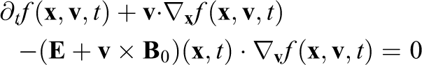
The Vlasov–Poisson equation describes the motion of a plasma in its self-consistent electric field for low-frequency phenomena. The Vlasov equation for electrons in dimensionless form is given as
The self-consistent field for electrons in a neutralizing ion background can be computed by the following Poisson equation
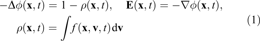
Here,
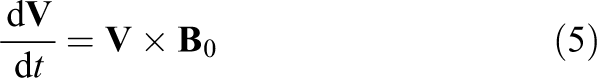
The characteristic curves of the Vlasov equation can be defined by the following system of ordinary differential equations (ODE)

Let us denote by

since the distribution function is constant along the characteristic curves.
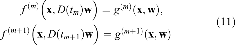
2.2. The semi-Lagrangian method for Vlasov–Poisson
To numerically compute the solution of the Vlasov equation, we use the so-called semi-Lagrangian method. We introduce a 6-D grid to discretize the phase space. In each time step, the equations for the characteristics are solved for each grid point backward in time from time
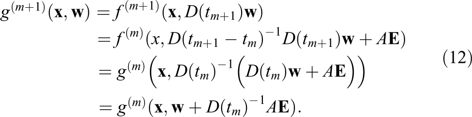
To efficiently solve the characteristic equations, Cheng and Knorr (1976) proposed a splitting method for the Vlasov–Poisson equation (
1. Solve
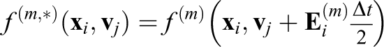
2. Solve

3. Compute
4. Solve
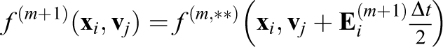
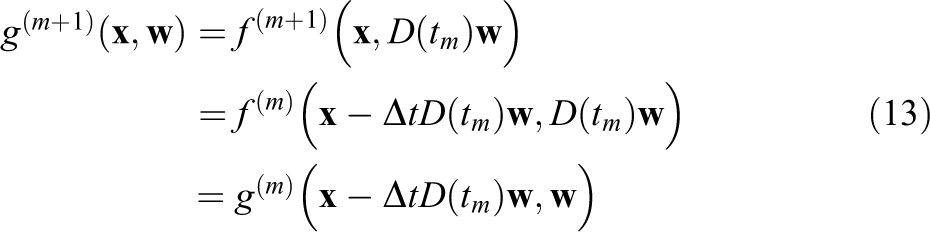
Note that the electric field is constant for the
To avoid 3-D interpolation, we use a cascade interpolation scheme replacing the 3-D interpolation by three successive 1-D interpolations. Moreover, we can use a first-same-as-last implementation that clusters step 4 of time step
As a consequence the main building block of the split-step semi-Lagrangian discretization of the Vlasov–Poisson problem is 1-D interpolation on 1-D stripes of the 6-D domain. Moreover, the interpolation step on the individual stripes has a special form: The function needs to be interpolated at a shifted value of each grid point and the value of this shift is constant for the whole stripe. For a stripe of length

Since
Advections can also be reduced to 1-D interpolation for the Vlasov–Maxwell equation using the backward substitution method introduced by Schmitz and Grauer (2006). In this article, we focus on the Vlasov–Poisson problem. However, we include strong background magnetic fields and discuss in the next section how they can be integrated into the split-step semi-Lagrangian scheme.
2.3. Split-step semi-Lagrangian method on a rotating mesh
In a magnetic confinement fusion device, the background magnetic field is strong compared to the self-consistent fields and causes a rapid motion around the field lines, the so-called gyromotion. Often the time scale of the gyromotion is the fastest so that we do not want to accurately resolve this time scale. On the other hand, the rotation around the magnetic axis (here the
We therefore propose the use of a rotating grid that follows the circular motion of the characteristics given by
Moving grids for Vlasov simulations have previously been discussed by Sonnendrücker et al. (2004), however, not in the context of parallelization.
To this end, we define a logical grid equivalent to the physical grid at initial time. Let us define the rotation matrix
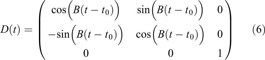
where
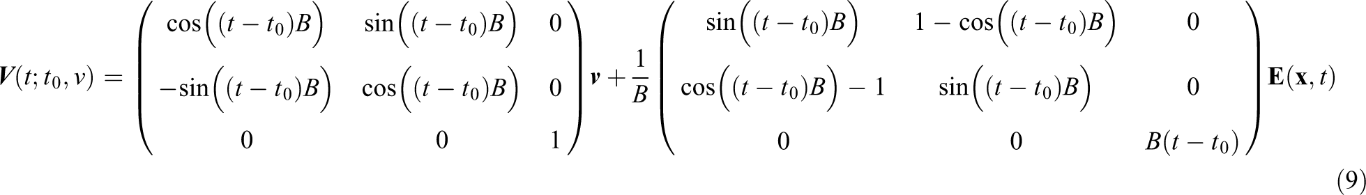
For a velocity

In the advection steps, we always solve the characteristic equations in physical coordinates and then transform the resulting velocity coordinates to the logical grid.
We again split the

This yields the following advection steps on the rotating grid:
for given
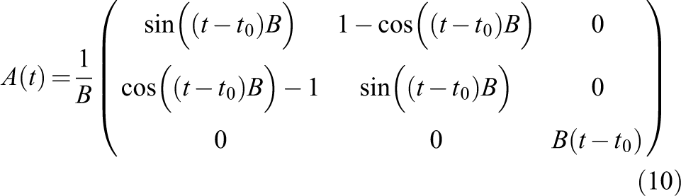
To find the representation of
Note that the displacement
Compared to the case with fixed grid, the displacements in
2.4. Domain partitioning
Due to the curse of dimensionality, the memory requirements of a grid in the 6-D phase space are rather high already for coarse resolutions. Therefore, a distributed numerical solution of the problem is inevitable. Two choices of domain partitioning are considered in this article: Domain decomposition (Crouseilles et al., 2009): The domain is decomposed into patches of 6-D data blocks, each representing a separate part of the domain. The patches are mapped to a 6-D logical grid of processors. For interpolations next to the domain boundary, halo cells with a width determined by the interpolation stencil have to be introduced and filled in advance with data from neighboring processors. This classical approach is widely used in parallelizations of lower dimensional physics and engineering problems, e.g. 2-D or 3-D computational fluid dynamics. Remap (Coulaud et al., 1999): Two decompositions of the domain are introduced, the first one distributing the domain only over the velocity dimensions (keeping the spatial dimensions local to each processor) and the second one distributing the domain only over the spatial dimensions (keeping the velocity dimensions local to each processor). For
The first strategy has the clear advantage over the remap method that the complexity of the communication pattern is reduced dramatically. On the other hand, the remap scheme is very well adapted to the split-step semi-Lagrangian method since the 1-D interpolations can be performed locally once the remapping has been applied. For the domain decomposition method, the 1-D stripes are usually distributed over separate domains. This makes the implementation more complicated and introduces an artificial time-step restriction (similar to a CFL condition) since the interpolation needs information of the function around the shifted data point
2.5. Solution of Poisson’s equation
The focus of this article is on the distributed solution of the 6-D Vlasov equation. However, in addition, we need to solve the 3-D Poisson problem (1). Since the problem is only 3-D, the compute time spent on its solution is almost negligible. For this reason, we use a pseudo-spectral solver based on fast Fourier transforms (FFTs) for the solution of the Poisson equation and remap the solution between domain decompositions that are local along the direction where FFTs are performed. In case a full 6-D domain decomposition is used (i.e. when the widths of all dimensions of the logical grid of processors are greater than 1), there are several subgroups of processors that span the whole
Finally, we also include a diagnostic step in our stimulations that computes scalar quantities like mass, momentum, and energy, thus containing reduction steps over the full 6-D array.
3. Interpolation on distributed domains
To compute the interpolated values, we can either use nodal interpolation formulas like Lagrange interpolation or global interpolants like spline interpolation. For simulations of the Vlasov–Poisson problem, cubic spline interpolation is most popular since it is well balanced between accuracy and efficiency. In combination with a domain decomposition, we however have to deal with the fact that the stripes are distributed between several processors, rendering a global interpolant impractical due to the required data exchange. Local splines as example considered for the 4-D Vlasov–Poisson equation by Crouseilles et al. (2009) are an interesting alternative. However, in this article, we focus on local Lagrange interpolation.
Let us recall the special structure of the interpolation task arising from our 1-D advections: The new value at grid point

Depending on the sign of
3.1. Fixed-interval Lagrange interpolation
Lagrange interpolation with a stencil that is fixed around the original data point
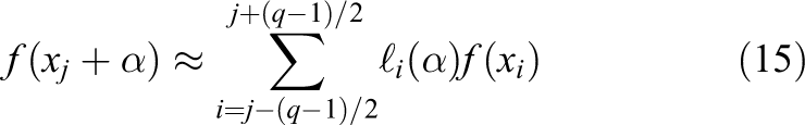
where
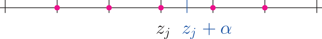
Fixed-interval Lagrange interpolation based on a five-point stencil. The red dots indicate the points necessary to calculate the value at
3.2. Centered Lagrange interpolation
As an alternative, we consider the Lagrange interpolation for an even number
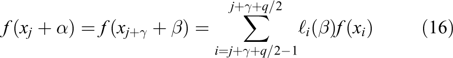
The choice of the data points for the interpolation stencil is illustrated in Figure 2 for a four-point-formula. In this case, we need to exchange a layer of
Centered Lagrange interpolation based on a four-point stencil. The red dots indicate the points necessary to calculate the value at
Having detailed on the mathematical background, we now turn toward a discussion of the aspects and challenges of an efficient implementation and parallelization.
4. Implementation and parallelization
Representing the 6-D distribution function on a grid requires a large amount of memory. Thus, it is of primary importance that an implementation can be efficiently distributed over a sufficiently large number of compute nodes to make use of the aggregate memory provided by the nodes. For the same reason, the problem is not very well suited to be solved on GPUs due to their scarce memory resources.
For our implementation, we use object-oriented Fortran 2008, the MPI for distributed-memory parallelism, and OpenMP directives and runtime functions to add shared-memory parallelism. 1 The developments were made within the framework of the library SeLaLib. 2 The 6-D distribution function is discretized on a 6-D Fortran array. Since a central idea of our method is dimensional splitting, the advection algorithms exclusively work on 1-D stripes of the 6-D data. Since these stripes are non-contiguous in memory for any direction but the first dimension, non-contiguous 1-D slices are copied from the 6-D array into a contiguous buffer before the interpolated values are computed. The performance of these strided memory accesses can be greatly improved by cache blocking as is discussed in Section 4.2.
For the domain-decomposition-based parallelization approach, the 1-D stripes are distributed over multiple processes. The following section discusses how the halo data are stored to perform the interpolations.
4.1. Distributed-memory parallelism
The domain decomposition approach requires a layer of halo cells around the processor-local data points to be able to conveniently compute the interpolants. In the discussion below as well as in our Fortran-based implementation, we consider global indices used locally in each MPI process.
A straight-forward way to handle the halos would be to include the cells into the 6-D array of the distribution function. Synonymously, this can be regarded as to work with 6-D arrays that overlap between neighboring processors. Padding the 6-D array with the halo cells has the advantage that the data are laid out contiguously in memory in the first dimension stripe-by-stripe, that is, the interpolation routines can work directly on the array in this special case. Stripes along higher dimensions are conveniently accessed via Fortran-style linear indexing, however, one has to keep in mind that the elements are laid out in memory in a strided fashion. It is important to avoid Fortran array slicing operators which cause temporary arrays to be used. Performance can be improved dramatically by implementing a cache blocking scheme using 2-D buffer arrays, see below. Moreover, using halos, there is no need for special treatment of periodic boundary conditions during the advection step.
A second possibility is to allocate the halo cells separately from the 6-D array of the distribution function, that is, there is no index overlap on the 6-D array between neighboring processes. Note that in this situation the halo buffers are identical to the MPI receive buffers.
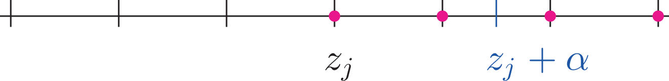
Figure 3 shows these two possibilities. In a 6-D array which includes the halo cells, one also has to allocate the corner points (displayed gray in Figure 3(a)) as well, even though they are not used by any of the 1-D interpolators. As is well-known, the volume of a hypercube mostly concentrates in the corners, therefore it is desirable to avoid memory allocation there. Moreover, in case the algorithm uses a different number of halo cells on different blocks of data, the 6-D array has to include the maximum number of halo cells in any direction. Therefore, we have chosen the second approach, using halo cells allocated separately from the 6-D array of the distribution function. It avoids the aforementioned disadvantages and is in particular superior with respect to memory efficiency. Moreover, we can also exploit the fact that we only need the halo cells along one dimension at a time. Once allocated, the halo buffers can be reused.
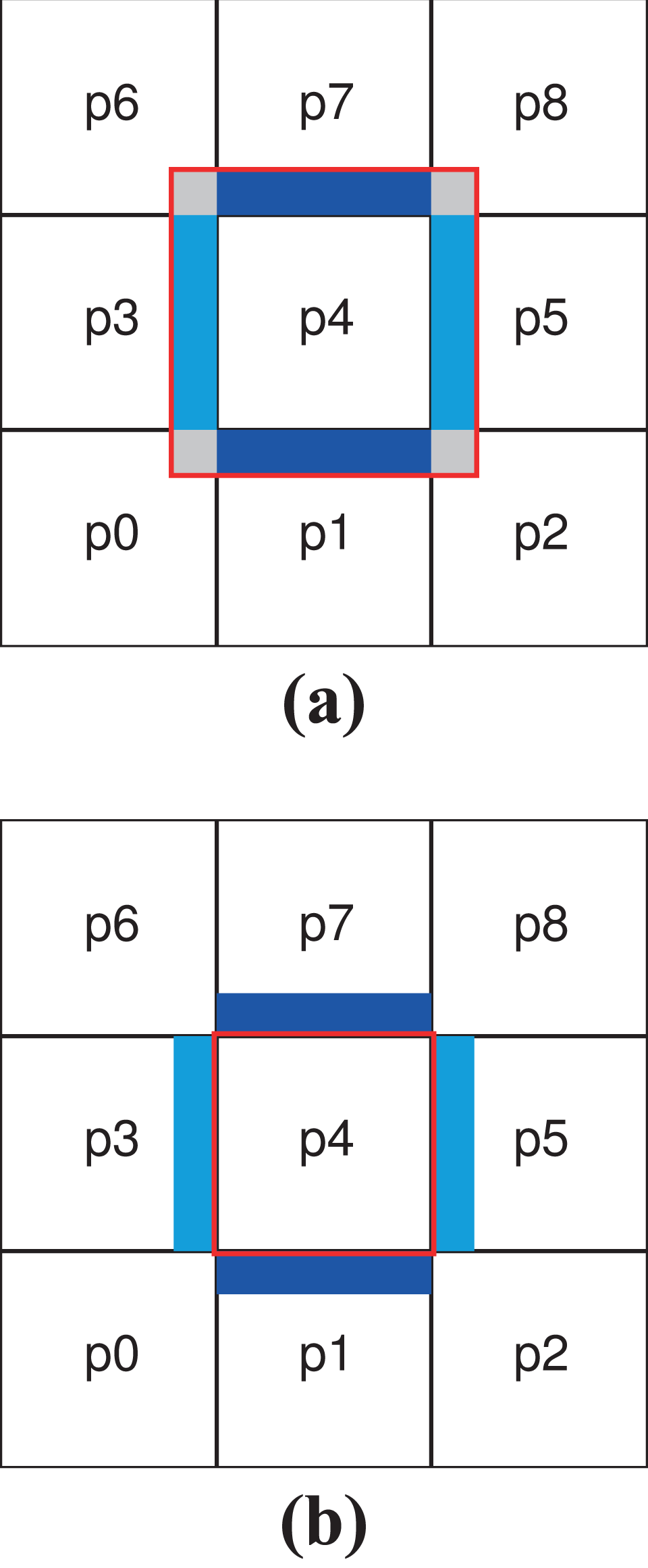
Schematic diagram of a data layout example, simplified to two dimensions and distributed over nine MPI processes labeled p0…p8. The square tiles represent the processor-local parts, the blue and cyan blocks the halo data needed for the advections along the first and the second dimension. The red square shows the data array stored by processor p4 for the two different data layouts. Layout (a) allocates the halo cells as part of the data array. Layout (b) allocates the halos as independent arrays. For layout (a), the gray blocks in the corners are unused. (a) Local arrays with indices that overlap between different processes and (b) local arrays with indices that do not overlap between different processes. MPI: Message Passing Interface.
If we assume a MPI-process-local grid of size
Table 1 compares the theoretical memory requirements for a typical process-local number of points per dimension for the two memory layouts. Note that the remap parallelization uses two 6-D data arrays for the two remap data layouts. The comparably low memory consumption of the domain decomposition implementation is especially advantageous on systems where fast memory is a scarce resource, for example, on certain manycore chips.
Comparison of the theoretical minimum memory requirements per MPI process for both algorithms under consideration.a
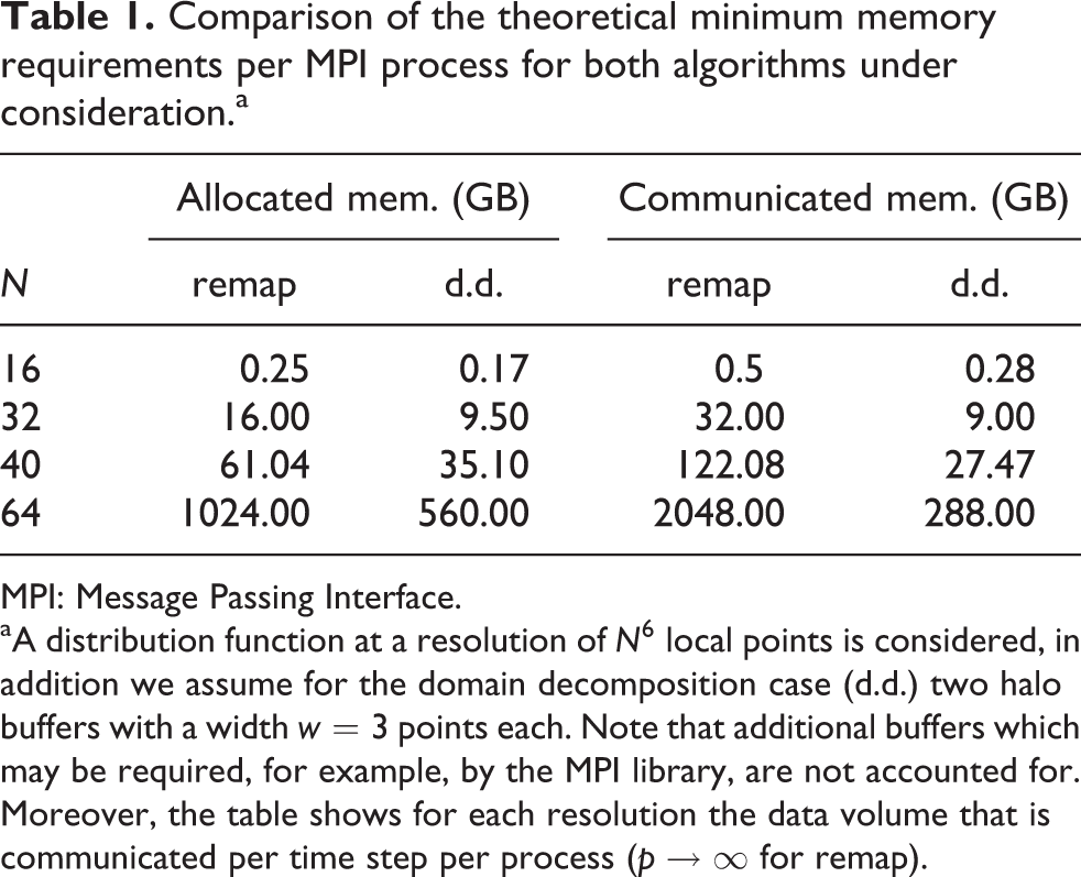
MPI: Message Passing Interface.
aA distribution function at a resolution of
Moreover, based on the numbers from Table 1, one can give a straightforward estimate of the resolution possible on a cutting-edge high-performance computing (HPC) system with approximately 100 GB memory per two-socket node. Considering the domain decomposition algorithm and putting two MPI processes per node with
4.2. Data access for 1-D interpolations
On the distributed domain, the advection along a dimension takes the form shown in Algorithm 1 at the example of
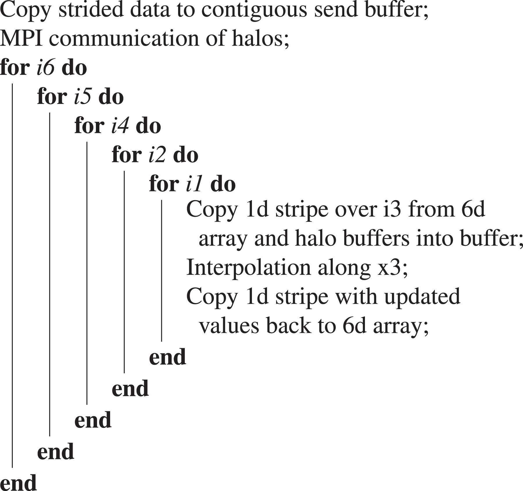
Advection along
The cache efficiency and the resulting performance can be greatly improved by a cache-blocking scheme similar to the schemes used to accelerate, for example, dense linear algebra operations. The blocking is based on a 2-D buffer array. Interpolations are performed along the first (contiguous) dimension. In the second dimension, the array is large enough to store at least a cache line of data. Algorithm 2 summarizes the loop rearrangements. A similar blocking has been implemented for all advection steps. For the advections along
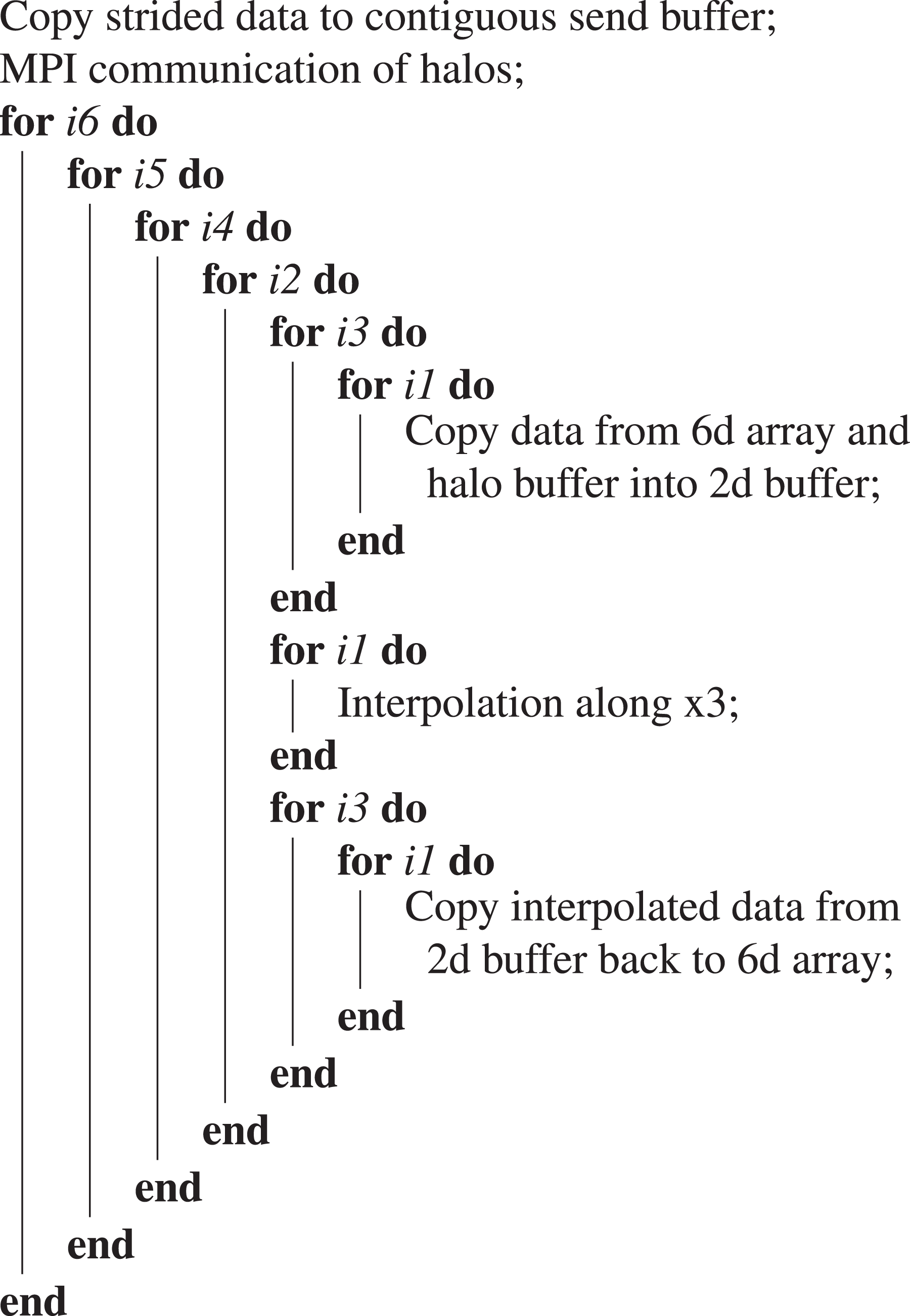
Advection along
4.3. Shared memory parallelization
Both implementations, remap and domain partitioning, are carefully parallelized using OpenMP directives and runtime functions to exploit the shared-memory architecture of prevalent multicore CPUs using threads, in addition to the distributed-memory parallelization which employs MPI processes.
A significant advantage of introducing a hybrid parallelization in addition to MPI is that it allows to reduce the memory consumption and the communication volume significantly. Instead of running one MPI process per available processor core, each allocating and exchanging halo cells, it is superior to launch only one or two MPI processes per socket, each with a proportionate number of threads pinned to the cores of that socket. All threads thereby share the halo cells.
Let us illustrate this effect by giving a simple numerical example. Consider a
We conclude that, first, it may be advantageous to use as few MPI processes as possible from the memory and communication point of view. Second, while the hybrid setup eliminates intra-node communication, the internode communication volume stays the same compared to the plain MPI case, with larger message sizes though.
A potential disadvantage of a naive hybrid approach is due to the fact that a significant fraction of the threads would be idle during the data-intense halo exchanges; however, by introducing an advanced pipelining scheme, we are able to hide the communication times to a large extent as is discussed in the following section.
5. Performance optimization
Performance optimization work aims at maximizing the node-level performance simultaneously with the parallel scalability that are conflicting goals to some degree. In the scope of this article, we target recent x86_64 systems with multicore or many-core CPUs as found in the vast majority of today’s HPC systems. Details on the systems under closer consideration are given in Table 2 in the following section where performance results will be discussed.
Specification of the hardware used for performance evaluation.a
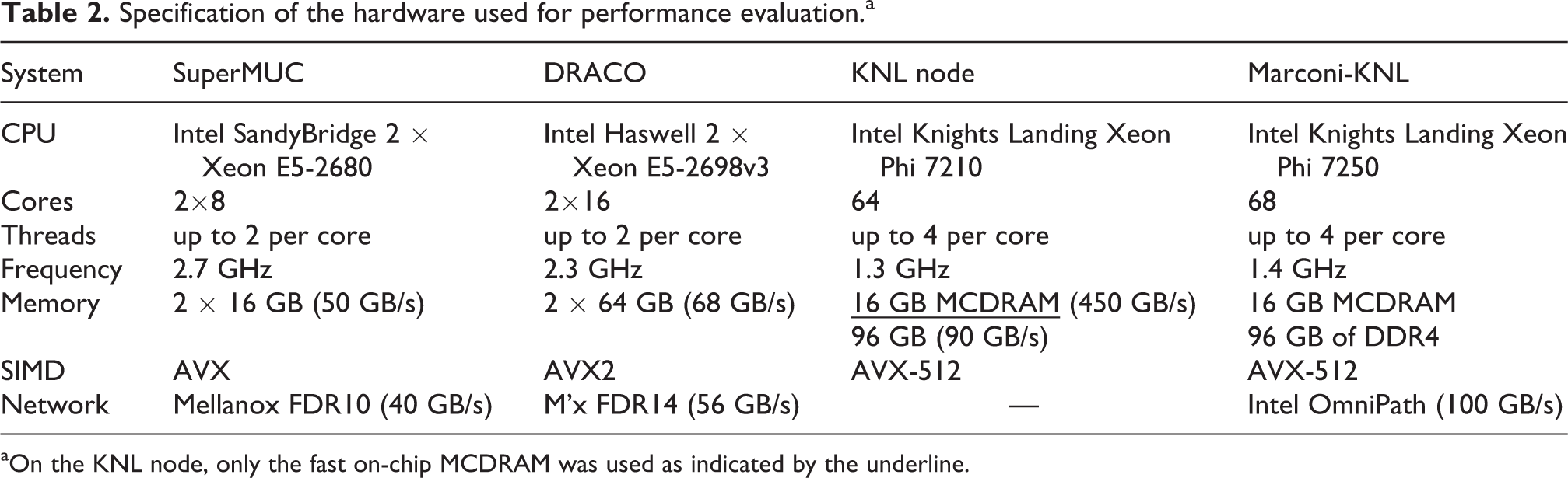
aOn the KNL node, only the fast on-chip MCDRAM was used as indicated by the underline.
5.1. Performance profile
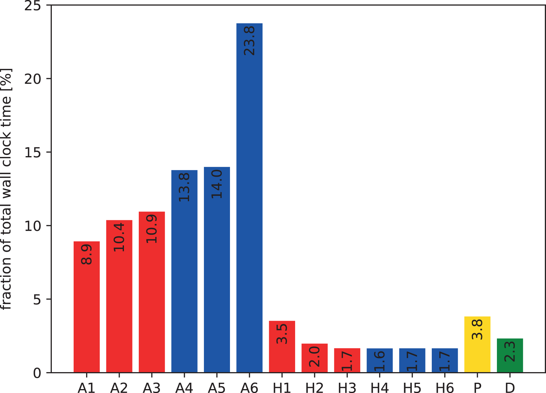
Figure 4 shows a breakdown of the costs of the various operations involved during a time step of the domain decomposition solver running on a single core without any parallelism. The profile is clearly dominated by the advection computations (“A”) including the Lagrange interpolation. Going from the direction of the first to that of the sixth dimension, the cost of the advection monotonically increases. This effect is caused by the fact that memory accesses become more and more strided. It is important to note that the effects of the striding are already mitigated by the cache blocking scheme that preserves a cache line, once loaded. Moreover, the prefetch efficiency of the processor appears to deteriorate with increasing strides. The preparation of the halo buffers (“H”), which also involves copies from strided into contiguous memory (however of much less data compared to step “A”), is by far less time-consuming. However, neighbor-to-neighbor MPI communication is included in “H” which becomes important when the parallelization spans multiple nodes. Finally, the Poisson-solve step and the diagnostics account for roughly 4% and 2% of the total runtime, respectively.
Profile of the domain decomposition implementation running a
In addition to simple and lightweight timing facilities, we used the tools Amplifier and Advisor from the Intel Parallel Studio XE package to obtain low level information on the performance and limitations of various parts of the code. Based on that information, code improvements were implemented, the most important of which are detailed below.
5.2. Single-core performance
Without considering MPI communication, the major factors limiting performance of both the 6-D Vlasov implementations, the remap and the domain decomposition, are due to the fact that the vast majority of the memory accesses—except the ones along the first dimension—are strided. A cache blocking scheme mitigates this issue significantly, as illustrated by performance numbers below. Nevertheless the code remains memory bound. The increase in runtime from “A1” to “A6” in Figure 4 reflects the aspect of the increasingly strided memory accesses.
In addition, single instruction, multiple data (SIMD) vectorization is a key factor to achieve performance on modern CPUs. While in early days (SSE2) only a factor of two was lost when vectorization was ignored for double-precision operations, the potential loss has grown to a factor of 4 (AVX) or 8 (AVX512) on more recent CPU models. We have implemented Lagrange interpolation routines such that the compiler is able to generate vectorized code that we verified carefully using compiler reports and performance tools. Arrays are aligned to 64 byte boundaries, though the large 6-D array of the distribution function is not padded in order not to waste memory. In general, the compiler is able to generate vectorized code for most of the loops.
Running 100 time steps of a
Finally, to quantify the effect of the cache blocking algorithm, the aforementioned test runs with 100 time steps take on the Haswell core in total about a factor of
5.3. Node-level performance
A modern compute node provides several cores that are organized in non-uniform memory access (NUMA) domains such that groups of cores share L3 caches and memory channels these cores can access fastest. Optimizing for the NUMA domains by careful process and thread pinning at runtime turns out to be important. Typically, MPI processes are pinned to sets of cores on sockets, and threads are pinned to individual physical cores from these sets. When overlapping communication and computation as introduced in the following subsection, it turns out to be advantageous only to pin the processes to constrain the threads within NUMA domains, and in addition, to use hyperthreads.
As the typical structure of the code are six-fold nested loops, a standard loop-based OpenMP parallelization strategy proved rather successful. From benchmark measurements at various resolutions, it was concluded that the runtime is minimized when the outer two loops are collapsed into a single one to increase the granularity of the parallel workload and when static loop iteration scheduling is used. Each thread is able to benefit from cache blocking and vectorization in the inner loops. Virtually any workload in the code is parallelized using that technique. As a result, the application scales well over a single node in pure OpenMP as shown in Section 7.
5.4. Distributed-memory performance
Semi-Lagrangian 6-D Vlasov solvers are unavoidably intense in terms of memory and data communication volume (cf. Section 4.1). For the domain decomposition approach, typical sizes of single MPI messages are in the range of
As outlined in Algorithm 2, each advection step starts with MPI communication to fill the halo buffers in the neighbor processes, before the interpolations are performed. We use standard blocking point-to-point MPI communication, in particular the
In hybrid-parallel setups the initial MPI communication would only keep a single thread busy while all the other threads were idle. The trend toward systems with increasingly more cores per socket suggests to use multiple threads per MPI process to overlap (“pipeline”) the communication with useful computation.
5.4.1. Simultaneous communication and computation
To implement pipelining of communication and computation, we block the data along a dimension different from the one we intend to interpolate along and perform data exchange and computation simultaneously on the resulting independent blocks, as illustrated in Figure 5.
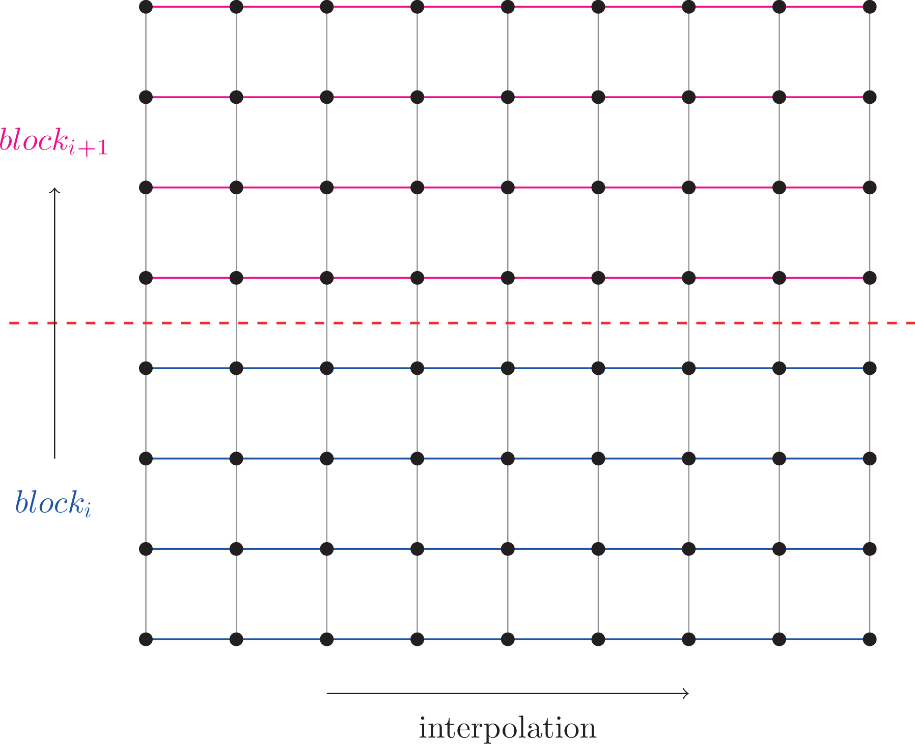
Blocking of a 2-D example grid, perpendicular to the direction along which is to be interpolated.
Here, we consider the Lagrange interpolation with fixed interval because in this case we do not have to handle additional blocking due to asymmetric data exchange. Moreover, to avoid a second layer of blocking, we do not consider blocks with different halo patterns. Anyway, the overhead introduced by not minimizing the halo widths for some blocks is less problematic when the communication is overlapped with computations.
For each data block, the advection computation consists of three steps: copy (generally non-contiguous 6-D) data into coherent buffer (C);
For each data block, these three steps need to be performed in the given order, but there is no dependency between different blocks. Nevertheless, we have to enforce some ordering to avoid a capacity overload of resources such as the maximum number of simultaneous hardware threads. Given the three-fold structure of the advection, we propose a straight forward pipelining scheme using three lanes as shown in Figure 6.
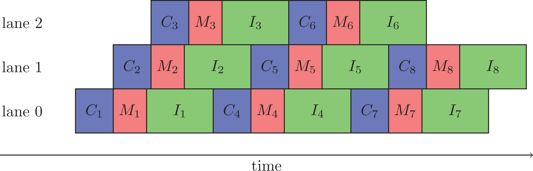
Schematic showing the temporal overlap of the copy operation (C), the MPI communication (M), and the interpolation (I) for a single MPI process at the example of an eight-fold blocked advection.
To keep the overhead of the start-up and the final phase as small as possible, we overlap communication and computation of advections for different dimensions as well. To give an example, let us start with the
5.4.2. Implementation details on the pipelining scheme
Our pipelining implementation relies on a thread-safe MPI library and on OpenMP threads—requirements that are provided by most modern compilers and libraries. The steps C, M, and I can be regarded as tasks with interdependencies.
In the following, we provide details on the implementation, referring to Algorithm 3. Initially, a list of all blocks is built, where each list element contains metadata such as block indices, the number of nested threads for the steps C and I, and two OpenMP locks, one for the C step and one for the M step. In the scheme proposed in the following, the orchestration of the tasks is explicitly controlled using a parallel region with a fixed number of three threads which uses internal loops with static scheduling and a chunk size of one such that the ordering is deterministic. For
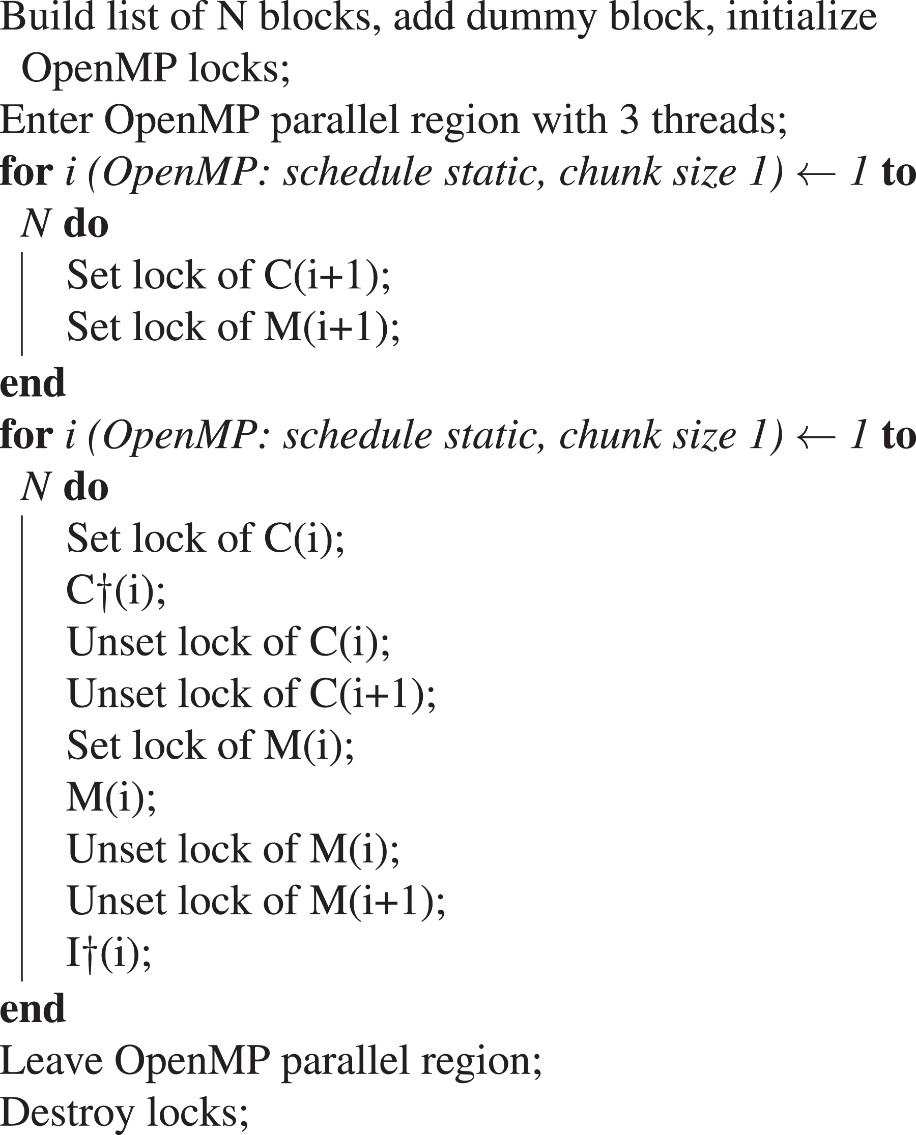
Control layer of the pipelining algorithm implemented using OpenMP directives and runtime functions. The symbol
At runtime, we have to specify two parameters that influence the performance of the implementation: the number of blocks and the number of threads used by each of the C and I tasks. The smaller the blocks are chosen the shorter the start-up and finishing phases become during which communication and computation cannot be overlapped. On the other hand, the blocks should not be chosen too small to keep the overhead low. As the second parameter, one needs to decide how to assign the available threads to the C and I steps. Note that the first C and the last I step may use more threads since they do not fully overlap with other operations. It turns out that the use of simultaneous multithreading (hyperthreading) is beneficial in concert with the pipelining scheme. The implementation assures that not more than the maximum available number of hardware threads are used to avoid congestion. The cost induced by the lock management is negligible compared to the computation, for example, for a typical number of four blocks per direction as shown in Figure 15 for real run data. In particular, the benchmark numbers show that the pipelined code is as fast as the non-pipelined code for small core numbers (cf. Figure 13) and is strongly superior when going to larger core numbers in a weak-scaling scenario (cf. Figure 14). A detailed discussion including benchmark results is presented in Section 7.
An obvious choice for the advections in
An alternative implementation based on OpenMP 4.0 tasks with an explicit dependency graph for the steps C, M, and I, in combination with non-blocking MPI communication had also been evaluated. However, this line of work was finally abandoned due to inferior performance. The major issue with this implementation was that the timing of the execution of the tasks differed strongly between different MPI processes, decided internally by the OpenMP task runtime. Using the tightly controlled loop-based scheme presented above, it was found that conventional blocking MPI communication in dedicated threads provides superior performance, reproducibility, and, moreover, has lower memory requirements.
5.4.3. Optimization of the halo-exchange communication
As pointed out before, the 6-D Vlasov solver is a highly communication intensive application, rendering good large-scale parallel scalability a difficult goal to achieve. From our experiments, we find that the implementation can scale well even when spanning multiple islands on a HPC system, if the process grid is laid out in an optimum way and communication and computation are pipelined.
The HPC systems under consideration have the network topology of a pruned fat tree. An island of the system is designed such that each node of the left half of the island is theoretically able to communicate with the corresponding node of the right half of the island simultaneously at the same bandwidth, termed the bisectional bandwidth. Going beyond an island, the bisectional bandwidth is reduced. Here, the blocking factor is decisive, which is, for example, 1:4 on a system used below, meaning that the interisland bisectional bandwidth is only a quarter of the intraisland one. We are therefore challenged with at least four levels of interconnection speeds between MPI processes, namely communication via shared memory on the same socket, intra-node communication via shared memory between different sockets, intraisland and interisland communication via the network.
In addition to the pruned fat tree topology, there are other topologies, for example, high dimensional torus interconnects. We would expect the 6-D domain decomposition algorithm to benefit highly from such networks because a reduced bisectional bandwidth is avoided, whereas on a pruned fat tree it turns out to be one of the major challenges to scalability.
It is crucial to optimize the Vlasov solver and also choose the problem setup for the network topology of the machine as well as possible to prefer fast communication paths for the largest messages, which is discussed in the following.
5.4.4. Process grid optimization
The ordering of the 6-D process grid can be chosen such that communication between remote processes is kept as small as possible. A batch system lays out the MPI processes in a certain pattern, often placing the ranks consecutively on the nodes, one island after the other. When constructing the 6-D process grid, the MPI ranks are placed in row-major (C) order, indexing processes
To go one step further, we have experimented with communication patterns between islands that are more balanced in the time dimension. This is done by mapping consecutive MPI ranks onto blocks of
It is important to point out that these process grid optimizations do not reduce the total amount of data that is to be communicated. We will turn toward possibilities to reduce the communicated data volume in the following section.
5.4.5. Reduction of the communication volume
The MPI messages sent between neighbor processes to fill the halos use by default 8 byte-wide double precision numbers. We have implemented the option to halve the communication volume and time by sending these messages in single precision, leading to an improved parallel scalability especially in interisland scenarios. However, one has to keep in mind that an additional error is introduced into the computation which requires careful validation. We therefore consider single precision messages an experimental tool.
When running the pipelined code in a hybrid fashion it turns out that—depending on the balance between threads and processes—a fraction of the threads is idle waiting for communication to finish. To continue along the lines of single precision messages, we have therefore experimented with floating point compression to further reduce the communication volume and time while utilizing the threads that would otherwise be idle. Naturally, a simple stream compression algorithm is not suitable to compress floating point data, rather a lossy algorithm tailored toward numerical data is required. The ZFP floating point compression algorithm, of which an implementation is freely available as a library, compresses blocks of 64 double precision numbers, taking the desired precision as a parameter (Lindstrom, 2014). The compression ratio achieved depends on the similarity of the numbers in the blocks. Adjusting the precision to match single precision, we typically observe a compression factor of approximately 4 for the halo data, improving parallel scalability over islands significantly. In particular, the compression step is rather expensive as will be shown briefly in the following. The compression option might become more relevant in the future when the per-node computational power continues to grow faster than the network bandwidth.
In Section 7, we present performance studies, detailing on the various challenges and the respective optimization approaches to tackle them.
6. Numerical experiments
Before we benchmark our implementation and demonstrate the scalability of the code, we consider representative test problems with and without a background magnetic field and discuss accuracy and time-step restrictions (CFL-like conditions) for the various Lagrange interpolations on distributed grids. For the tests we look at the electric energy,
6.1. Vlasov–Poisson simulations
We first consider two test problems with no magnetic field, weak Landau damping, where the chosen resolution yields rather good accuracy, and a bump-on-tail instability with larger phase-space error, and compare the accuracy of the Lagrange interpolators of various order.
The initial value of the weak Landau damping problem is given as
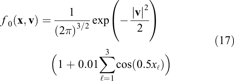
The grid resolution is chosen to be
The bump-on-tail test case has the initial value
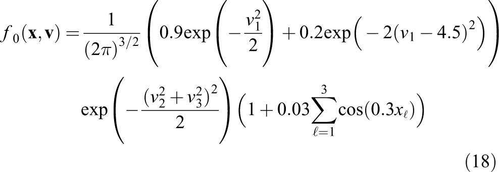
and is solved on a mesh with 32 points per direction until time 15. The reference solution is simulated on a mesh with 40 points per direction, a time step of
Figure 7 shows the error in the electric energy as a function of the time step for various orders of the Lagrange interpolator for the weak Landau damping example. Comparing the curves, we see that the error for the largest time step
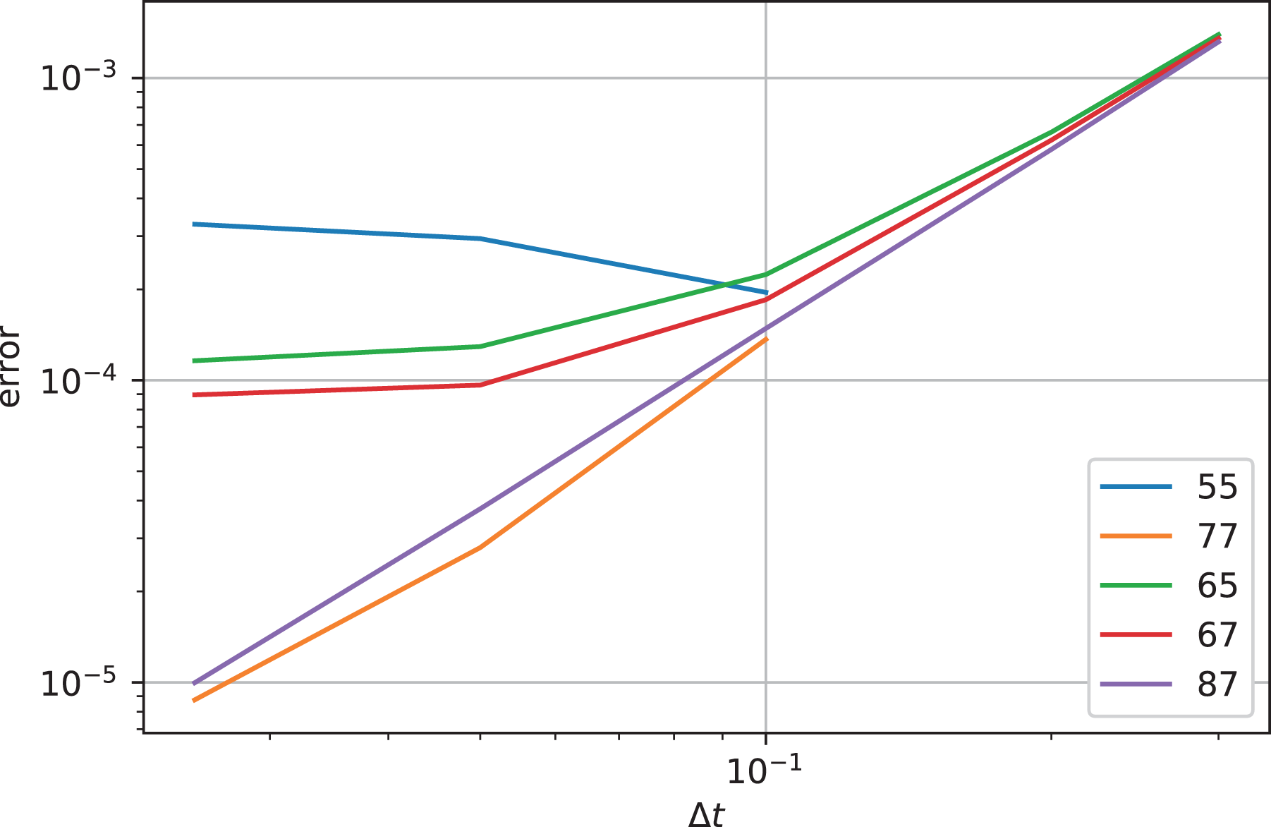
Landau damping: error in electric energy as a function of the time step for various interpolators. The numbers indicate the stencil widths of the
For this example, the displacement of the
Figure 8 shows the results for the bump-on-tail test case. In this case, the spatial error is larger which is why larger time steps compared to the value of
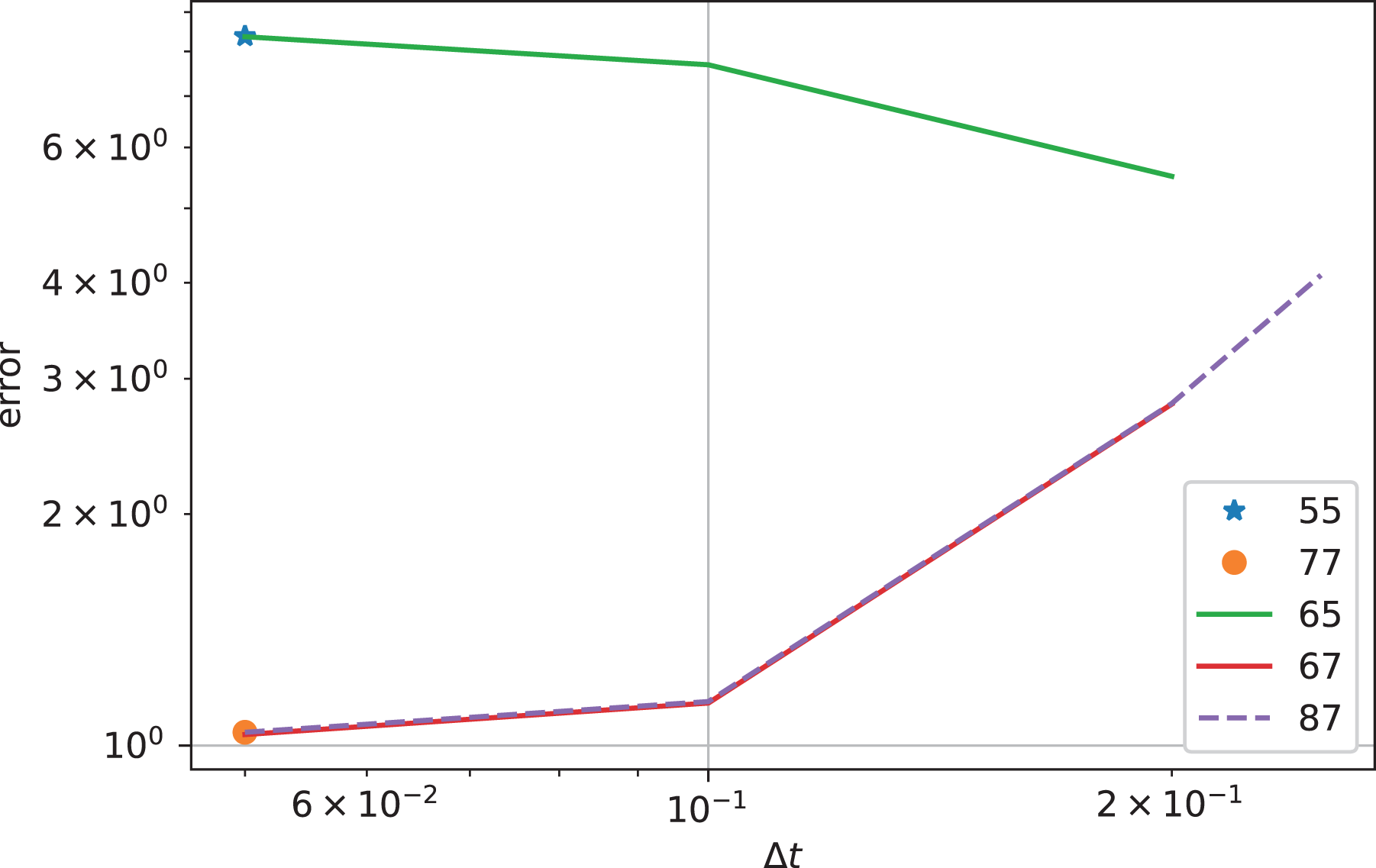
Bump-on-tail: error in electric energy as a function of the time step for various interpolators. The numbers indicate the stencil widths of the
Figure 9 shows the accuracy as a function of the wall clock time for a simulation on a single node of the DRACO cluster with 32 MPI processes for the Landau case. We can see that the computing time increases with the order but the increase is very small. On the other hand, the increasing halo cells for increasing order will impact the performance more strongly when MPI communication between nodes is involved.
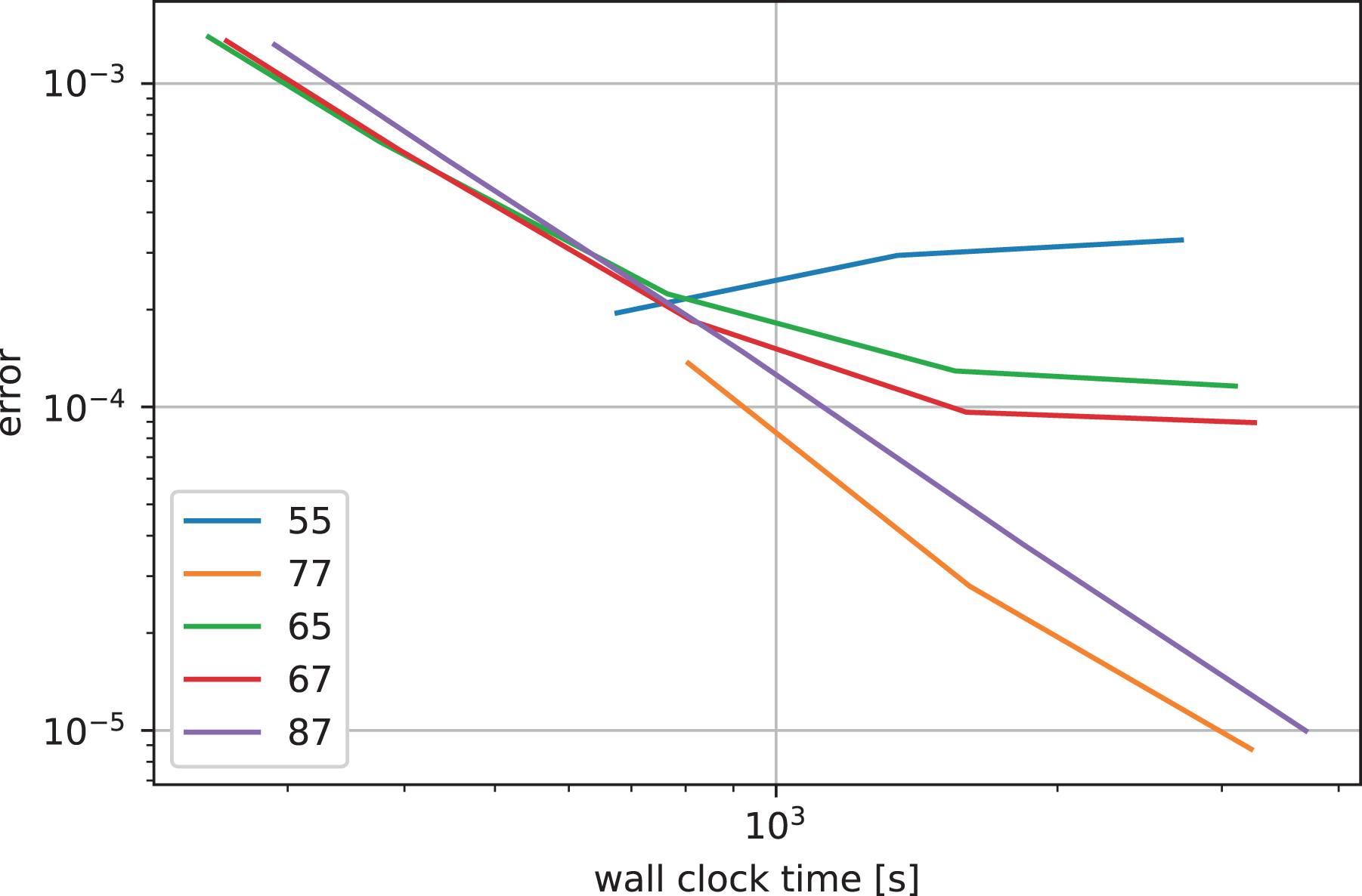
Landau damping: error in electric energy as a function of the wall clock time for various interpolators. The numbers indicate the stencil widths of the
We conclude that the time step should be chosen around the CFL-like condition or even somewhat above it (enabled by the use of one-sided halo blocks as described in Section 3.2) and that an integrator of order five and below does not yield the necessary accuracy at that temporal resolution.
6.2. Simulations with rotating mesh
As an example of a simulation with a strong background magnetic field

In this case, the gyrofrequency is given by
To understand the time-step restrictions of our distributed memory parallelization with the rotating grid, we estimate the maximum displacement in the various advection steps. The displacement of an
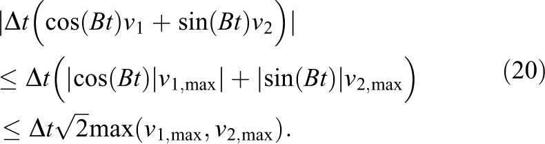
Here, we use
The displacement of the velocity advections depends on the electric field. The electric field induced by the initial condition is given as
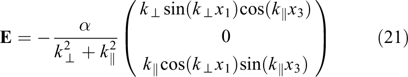
If the electric field is damped in time, we can estimate the electric field by
Let us consider the following parameters,
The maximum displacement along
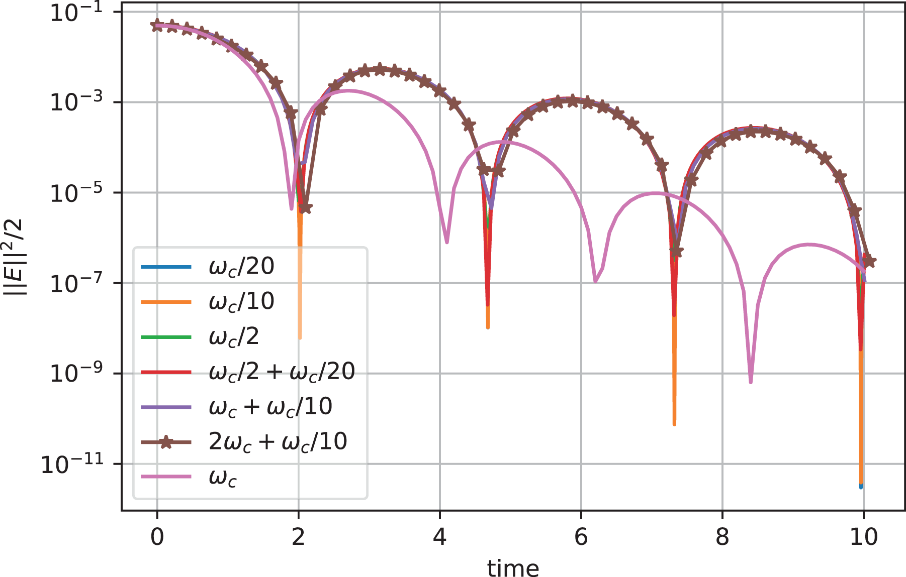
Simulation with rotating velocity grid: electric energy as a function of time for various time steps (given in the legend).
7. Performance benchmarks
To systematically compare and evaluate the performance and the scalability of the remap and the decomposition implementations, a series of runs was performed, going from a single compute node to a HPC cluster and further up to multiple islands on a supercomputer. For most of our basic tests and during iterative performance optimization work, we used a two-socket Intel Haswell-type node, the building block of the DRACO HPC cluster at MPCDF. 3 Moreover, an Intel Xeon Phi KNL node was available, running in “flat” mode with the 16 GB of MCDRAM available as a separate memory domain. All the runs performed on the KNL used the fast MCDRAM exclusively. Finally, we present large-scale runs performed on the SandyBridge partition of the SuperMUC HPC system of the Leibnitz Supercomputing Center, covering up to eight islands with 64k physical cores. Table 2 provides details on the specifications of the compute nodes.
The Landau damping test case was chosen in each run. We consider a seven-point Lagrange interpolation for both
To compile and link the code, recent versions (16 and 17) of the Intel compiler were used throughout this work, with the optimization flags set to
7.1. Node-level performance
To evaluate the performance of the OpenMP-based parallelization in comparison to MPI, we present scalings on a single compute node in this section.
Each run was repeated five times to average out small variations between individual runs that were found to be on the order of up to 5%. A problem size of
Moreover, the simulation of a
Figure 11 shows strong scalings on the Haswell-type node. For both, the domain decomposition and the remap case, a scan in the number of MPI tasks keeping the number of threads fixed to 1, and for comparison, a scan in the number of OpenMP threads with a single MPI process are shown.
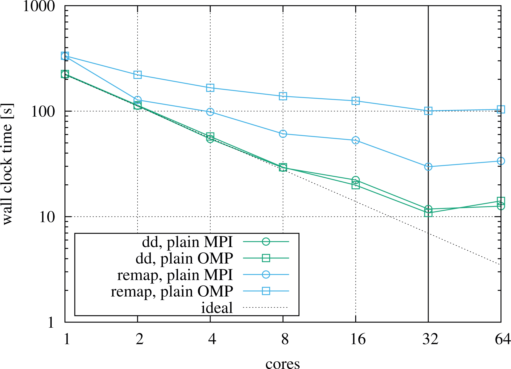
Strong scaling in pure MPI and pure OpenMP on the Haswell node, comparing the domain decomposition code with the remap implementation, running five time steps of a
For each series, the optimum pinning strategy is chosen, which has been determined experimentally a priori. The MPI processes are pinned in a round-robin fashion between the two sockets. Doing so, the memory bandwidth of both sockets is used as soon as more than one process is run. Only MPI messages are transferred via the link between the sockets. On the other hand, the threads for the OpenMP scan are pinned in a compact fashion to physical cores, filling the first socket completely before going to the second socket. The compact OpenMP thread pinning strategy reduces the traffic over the link between the two NUMA domains significantly. Note that a thread-aware first-touch memory allocation and handling is not possible when traversing the 6-D array of the distribution function in all the six directions.
Figure 11 shows that for the domain decomposition runs, both the MPI and OpenMP results are very similar and scale virtually ideally up eight cores. They continue to scale well up to the full
The remap code performs significantly worse than the domain decomposition implementation. Running on the full node with 32 MPI processes, it is about a factor of
For comparison and to include results from a many-core platform, we show numbers based on the identical
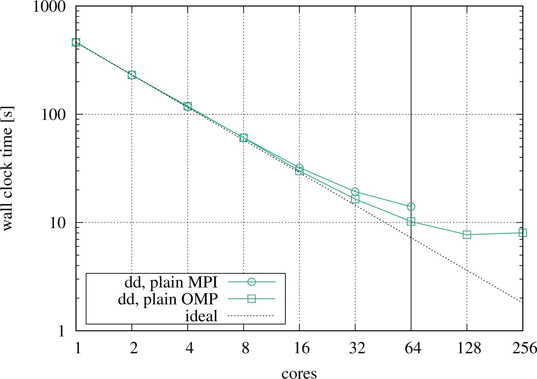
Strong scaling in pure MPI and pure OpenMP on the Xeon Phi node. For comparison, the same setup as the one used for Figure 11 is run. The vertical line indicates the transition to simultaneous multithreading. MPI: Message Passing Interface.
Table 3 compares the node-level performance of the domain decomposition runs between the Haswell and the Xeon Phi node. Merely based on the ranked timings, the performance advantage of the KNL node relative to the Haswell node is roughly
Overview on the node-level performance by listing the 10 fastest runs on each platform.a
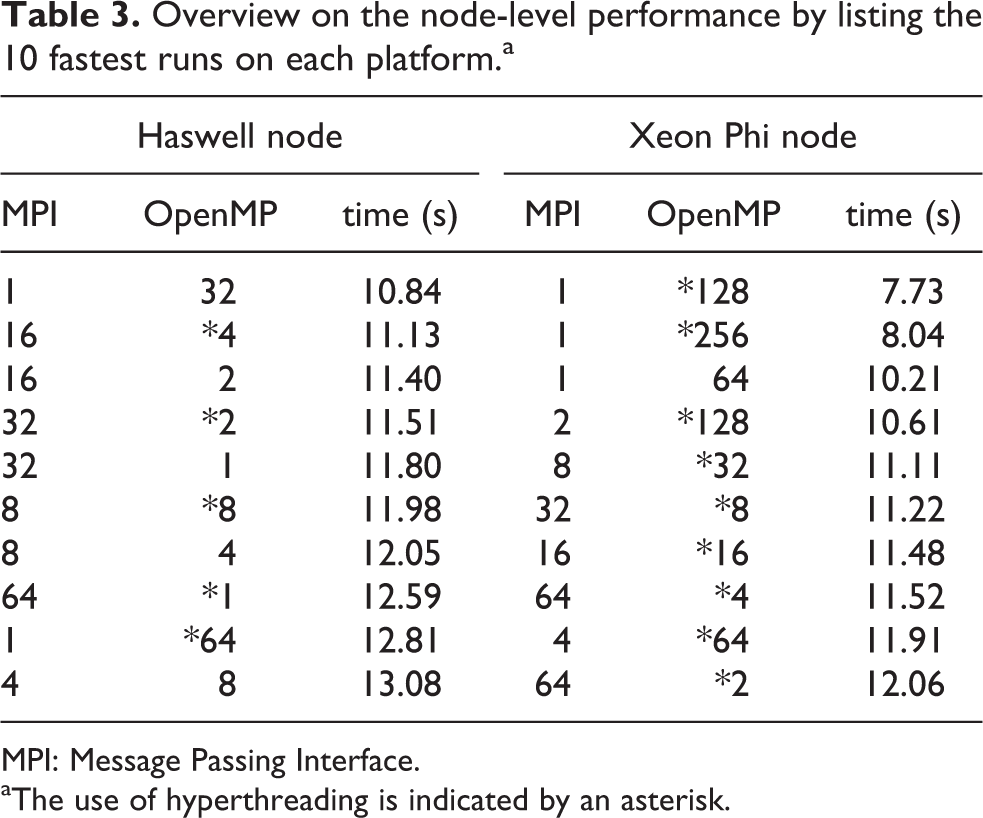
MPI: Message Passing Interface.
aThe use of hyperthreading is indicated by an asterisk.
In summary, both, the distributed-memory and the shared-memory parallelization of the domain decomposition implementation were found to scale very well on a single node. OpenMP threads and MPI processes can virtually be used interchangeably when running the domain decomposition implementation. This is an important finding relevant to the larger setups on many compute nodes that rely on hybrid parallelization, for example, running one process per socket and keeping all the available cores busy with threads, as presented in the following section. However, in practice for a given setup, it may not be beneficial to arbitrarily swap threads and processes due to implicit changes in the partitioning of the numerical grid and the process grid that may taint the performance in some cases.
7.2. Parallel performance
7.2.1. Medium-scale runs
In this section, we focus on the parallel performance of the 6-D Vlasov code on distributed-memory HPC clusters. We mainly consider the domain decomposition implementation but draw some comparison to the remap code as well.
First, we discuss medium-sized scaling runs performed on the DRACO HPC machine at MPCDF, mainly to investigate the scalability of the hybrid implementation. It consists of Haswell nodes as detailed in Table 2 in the previous section. The nodes are grouped into islands of 32 machines and are connected via an FDR14 InfiniBand network. The maximum job size is 32 nodes with 1024 physical cores in total, supporting up to 2048 simultaneously active threads. Note that the minimum number of MPI processes for which the domain decomposition implementation communicates with all the process neighbors via MPI messages is 64 which is therefore taken as the baseline for all scalings.
To be able to include the domain decomposition code with pipelining, that is, overlapping of computation and communication, into the comparisons in a fair way, we allow each process to use two hyperthreads even in a plain MPI run, since the pipelining scheme relies on having multiple active threads per process to work properly. For the other two codes under consideration, the effect of the two hyperthreads is negligible as shown in the previous section on the single-node performance.
We now turn toward a strong scaling before the more relevant weak scaling scenario is considered in greater detail. Figure 13 shows strong scalings in plain MPI and also for hybrid setups, going from 64 cores on two nodes up to the full island size of 32 nodes. The test setup uses a resolution of
Strong scaling on DRACO using seven-point Lagrange interpolation, running a resolution of
The hybrid parallelization turns out to be efficient when going beyond a single compute node as well. Figure 13 shows strong scalings for hybrid runs of the domain decomposition codes in direct comparison to the MPI runs, reducing the number of MPI processes by a factor of 1/2 or 1/4 and increasing the number of threads by the inverse factor. Note that hyperthreads are used in the example, that is, two threads share the same physical core. As can be seen, the hybrid curves follow the plain MPI curves very closely. For the largest runs, the hybrid case with eight threads per MPI process turns out to perform best for the domain decomposition code without pipelining.
An important effect induced by the multidimensional domain decomposition has to be recalled at this point to explain the deterioration of the strong scaling. As the global problem size is kept constant, the fraction of the distribution function that has to be communicated between neighbors increases as the strong scaling is performed due to the decrease in local grid size. This effect can be mitigated to some degree by performing hybrid runs. On the other hand, for the remap implementation, the total volume of communicated data stays constant, whereas the number of MPI messages increases quadratically with the number of processes.
These strong scaling curves are mainly given for reasons of completeness. As high memory demands in combination with low arithmetic intensity are the main challenges to be tackled when dealing with the 6-D Vlasov–Poisson problem, we turn toward the weak scaling properties of the codes that are more relevant to Physics simulations on large grids.
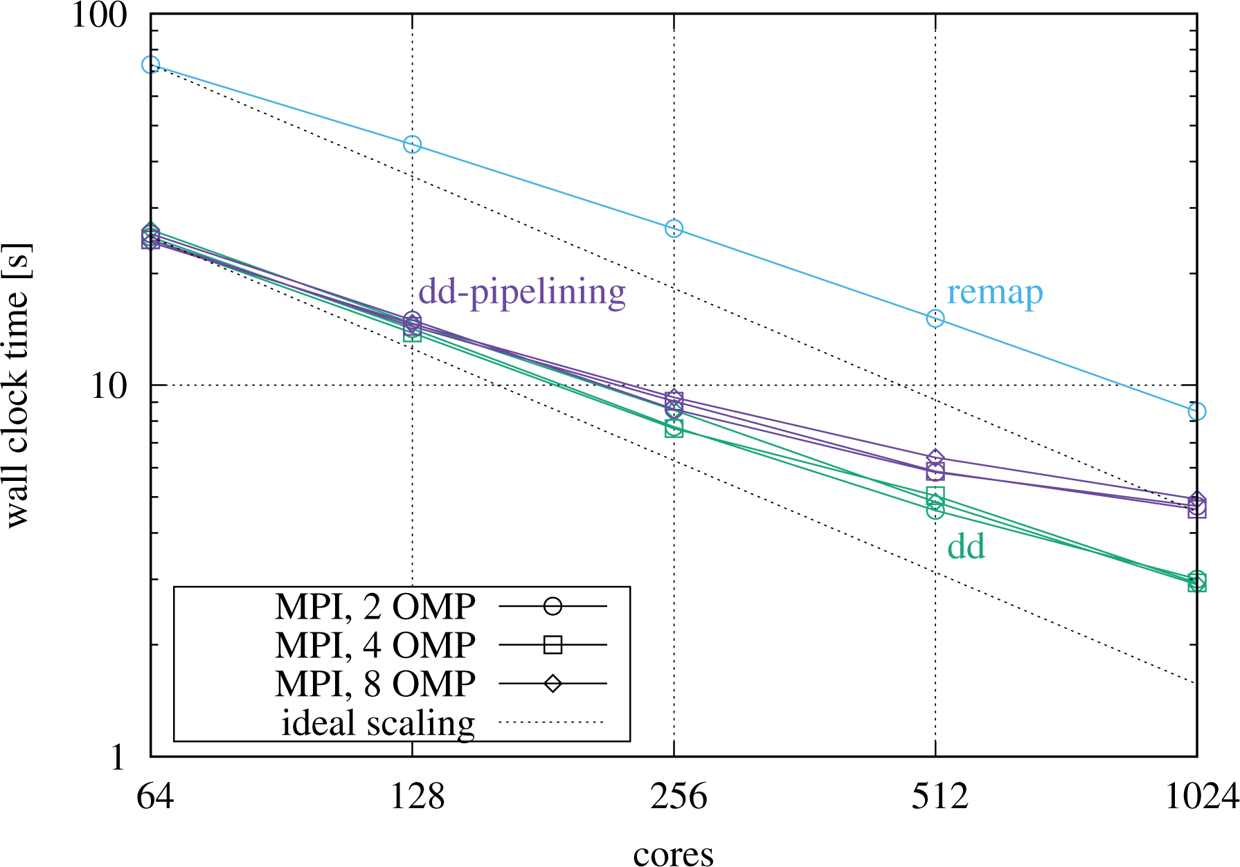
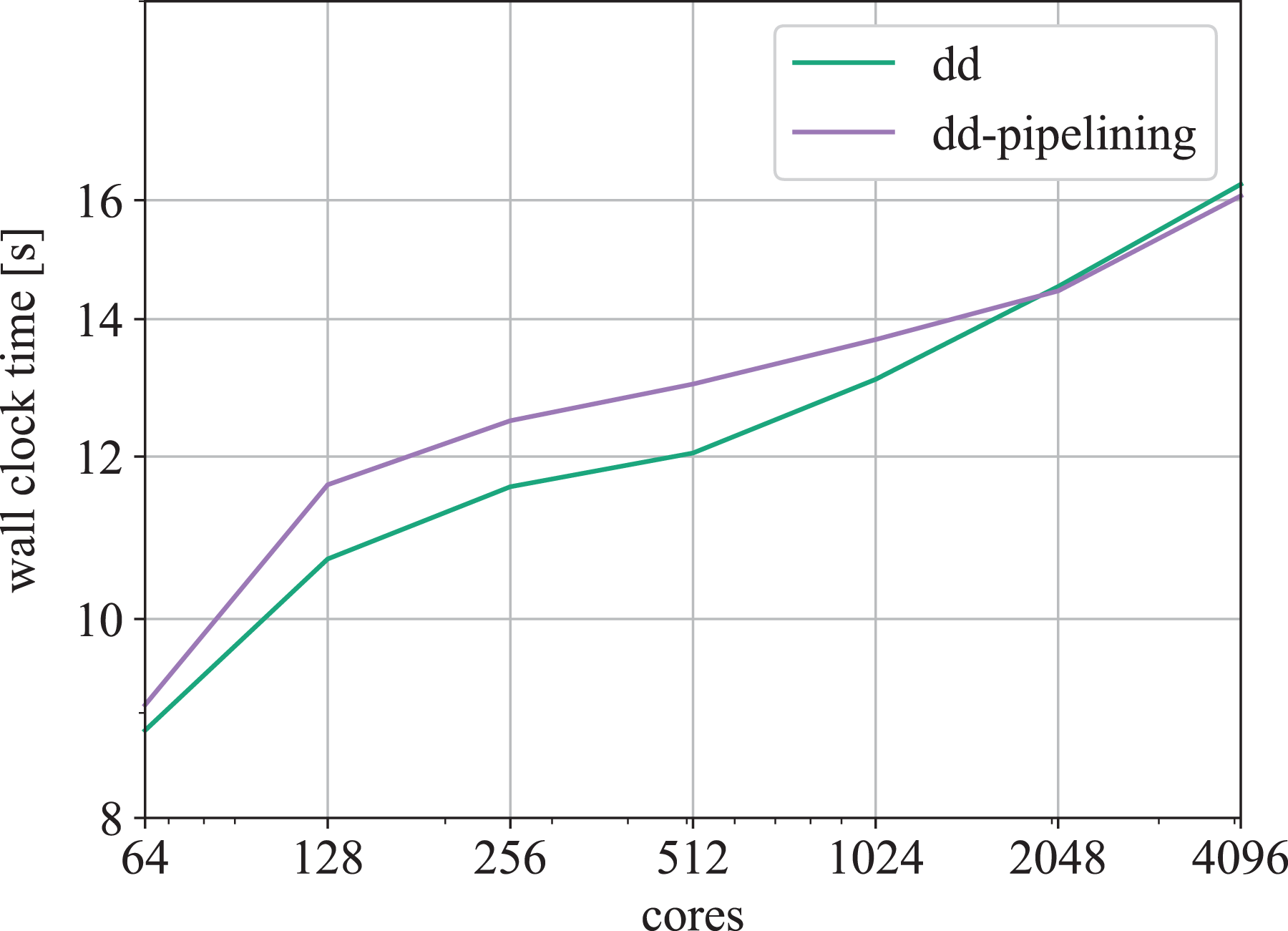
Figure 14 shows a weak scaling, starting on two nodes and keeping a workload of
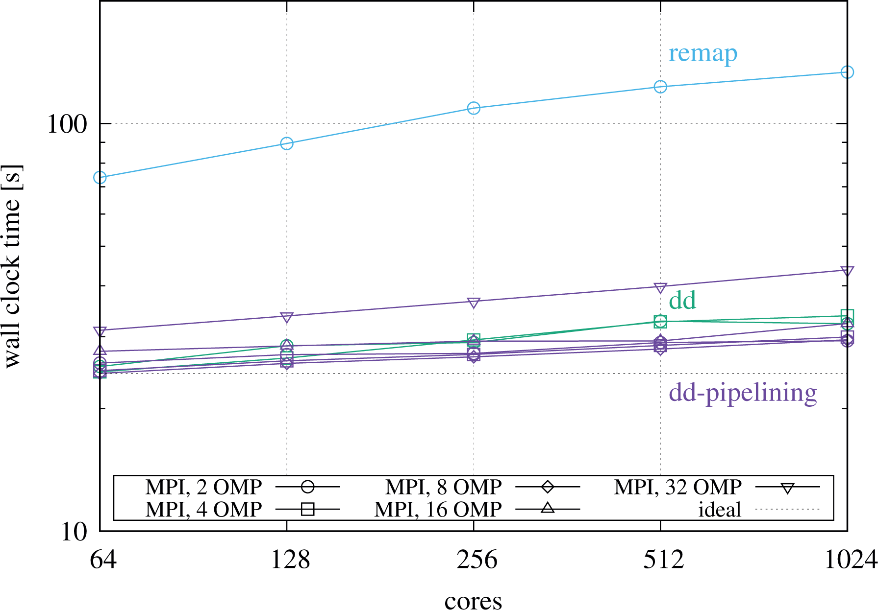
Weak scaling on DRACO using seven-point Lagrange interpolation, keeping a local problem size of
In addition to the plain MPI cases, the plot shows a selection of hybrid cases, exchanging processes with threads but operating on the same workload for comparability. The graph yields the important finding that hybrid setups running four or eight threads per process may be in fact the best choice for the pipelining code, which is in this situation able to utilize several threads for each the advection and the buffering tasks in parallel, while performing MPI communication at the same time, thereby hiding parts of the communication behind useful computation. As can be seen in addition for the pipelining implementation, the hybrid parallelization performs very well over a broad range of configurations. Even running only two MPI processes per socket (labeled “16 tpp”) turns out to be very close to the case with one MPI process per physical core (labeled “2 tpp”), less aggressive hybrid setups being located in between. However, reducing further to only a single process per socket (labeled “32 tpp”) causes the time to solution increase significantly which is caused by the fact that a single simultaneous MPI operation per socket is not sufficient to saturate the network interface. Finally, it has to be recalled that each hybrid configuration uses a different, optimal, process grid on top of the same numerical problem setup, which leads to different communication patterns that contribute as well to the variation observed between plain MPI and hybrid runs.
Concerning the weak scaling, the rise in the wall clock time is attributed to a significant part to the fact that halos in more and more spatial directions are communicated via the network instead of being shared via the memory on the node, as the system size is increased. An illustration and in-depth explanation will be given in the following section dealing with scalings on SuperMUC using a component-wise breakdown of the runtime.
To illustrate the behavior and performance of the pipeline implementation, time traces in a task-style are presented in Figure 15. In Section 5.4, the pipelining scheme was explained by means of the schematic Figure 6 which is hereby complemented with timing data. The run under consideration uses 64 MPI processes in total, employs two processes per node, one per socket, and uses OpenMP threads to keep all the cores busy. The plot shows timings obtained from the control loop which implements the pipelining scheme using three lightweight threads, indicated here by three lanes. Temporal overlap is possible between the lanes within the
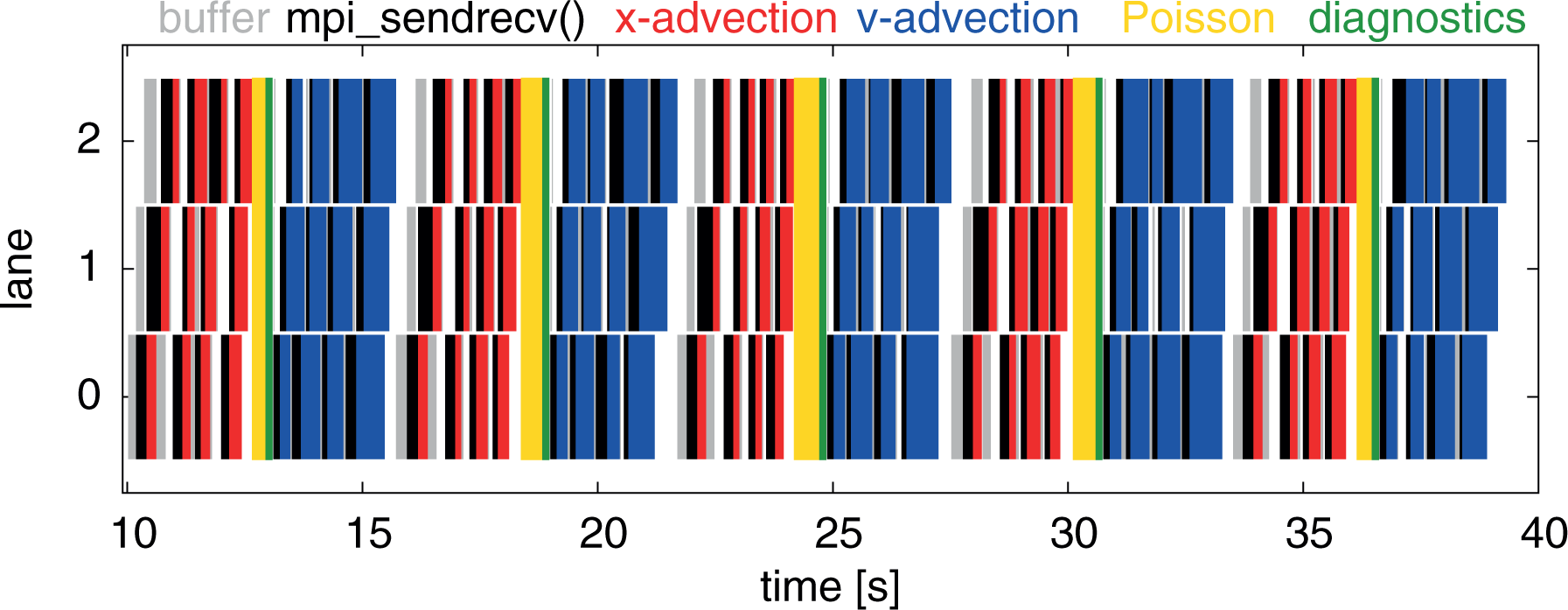
Timeline view on a hybrid pipelining case, running 64 MPI processes on 16 nodes, with two MPI processes and 16 hyperthreads per socket, picked from the runs shown in Figure 14. MPI: Message Passing Interface.
In the following section, we discuss runs on a supercomputer at large scale, also shedding more light on the effects which limit the parallel scalability.
7.2.2. Large-scale runs
To further evaluate the performance of the domain-decomposition-based solver, we present runs performed on the SuperMUC HPC system of the Leibnitz Supercomputing Center. 4
On the so-called phase 1 partition of the SuperMUC system, each node is equipped with two Intel E5-2680 CPUs (SandyBridge-EP) with eight physical cores, each supporting two threads per core (cf. Table 2). There are 512 nodes per island, connected via an InfiniBand FDR10 network. The blocking factor of the network between islands is 1:4. In total, 18 islands are available. In the following, we present scalings going up to eight islands with 64 k physical cores and 128 k hardware threads.
The resolution of the test case considered for the weak scaling on SuperMUC is
Figure 16 shows weak scalings for the remap and the two domain decomposition codes. There is one MPI process per physical core with two hyperthreads each. These extra hardware threads are enabled to include the pipelining implementation into the comparison.
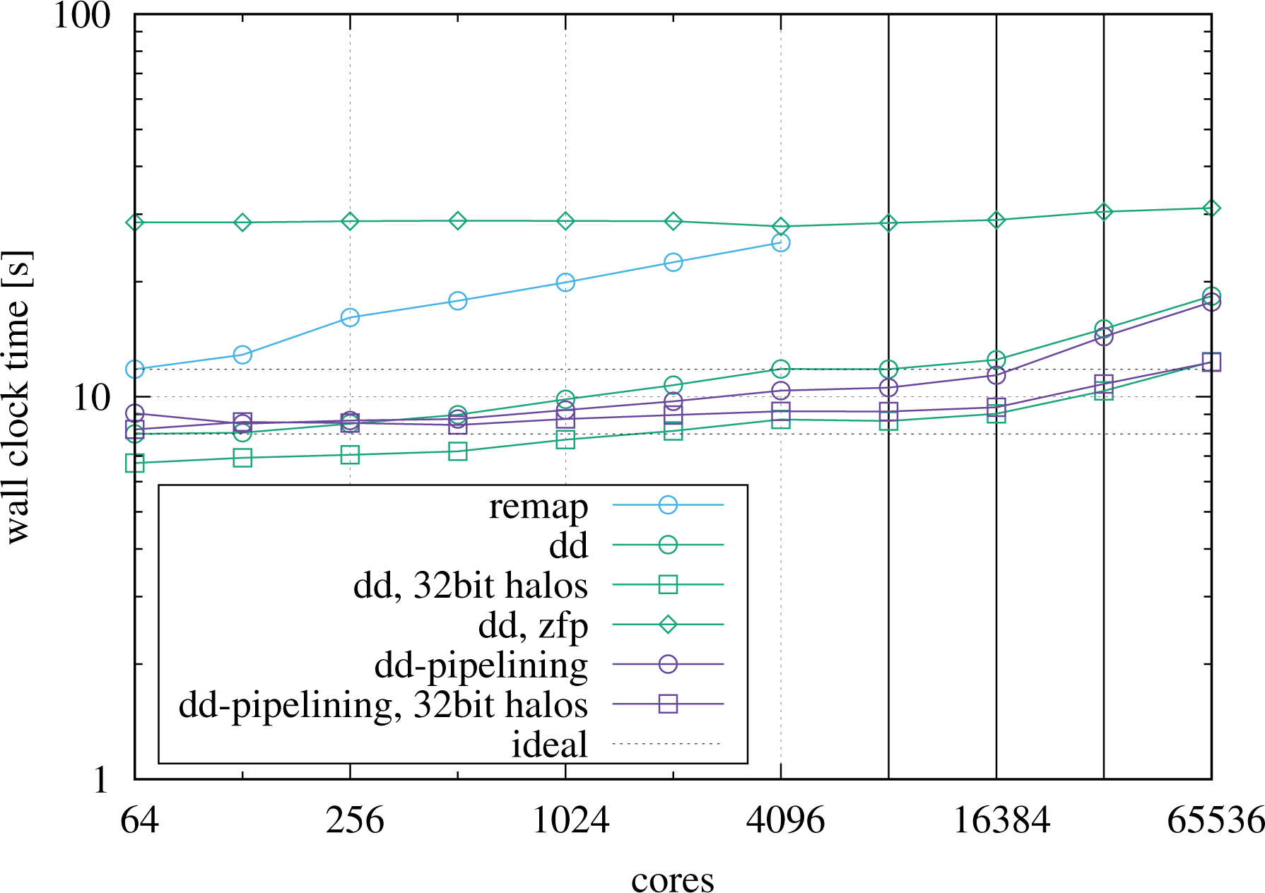
Weak scaling on SuperMUC comparing the domain decomposition codes with and without pipelining to the remap implementation, running one MPI process per physical core, with two hyperthreads each. The transitions going from 1 to 2, 2 to 4, and 4 to 8 islands are indicated by vertical lines. MPI: Message Passing Interface.
The results show that the domain decomposition codes both scale quite well. The plain domain decomposition implementation turns out to be faster than the pipelining one up to 512 MPI processes when the latter takes over. Going beyond the island boundaries leads to an increase in the wall clock times which is moderate at two islands but becomes more significant when going to four or eight islands. When scaling up, the increase in the wall clock time is mainly caused by the fact that an increasingly larger fraction of the halo data is exchanged over the network between nodes and finally between islands as the problem size is increased. The SuperMUC system has a pruned tree network with a blocking factor of
Compared to the domain decomposition codes, the remap code is slower, as already known from the previous tests. In addition, it scales slightly worse. More details on its scalability limitations will be given below. Due to a restriction in the implementation, the Poisson step currently prevents to use more than 4 k MPI processes.
In addition, the weak scaling plot Figure 16 contains data from two experiments aimed at increasing the parallel scalability by reducing the size of the MPI halo messages. The first experiment (labeled “32bit halos”) simply sends the halo data in single precision, thereby halving the communication volume. The wall clock time is significantly reduced and also the scalability is improved to some degree, especially when going from one to two islands. The second experiment (labeled “zfp”) takes one step further by applying a lossy compression to the halo data, thereby effectively reducing it to about a quarter of its size while preserving single precision accuracy. This comes at a significant computational cost but at the same time leads to a virtually flat scaling with nearly 100% parallel efficiency, even when crossing island barriers. Interestingly, at 4096 MPI processes, the runtime of the remap code is already very close to the one of the domain decomposition code with ZFP compression enabled. As hardware standards evolve, it is to be expected that the penalty of the ZFP compression becomes less and less important for hybrid runs on present and future systems with greater relative compute power compared to the network bandwidth.
Hybrid setups, that is, swapping MPI processes in favor of OpenMP threads for the domain decomposition code, did not turn out to be better than plain MPI cases on SuperMUC with its comparably small number of cores, in contrast to DRACO as shown before. As argued already for ZFP, the hybrid feature will become more important in the future.
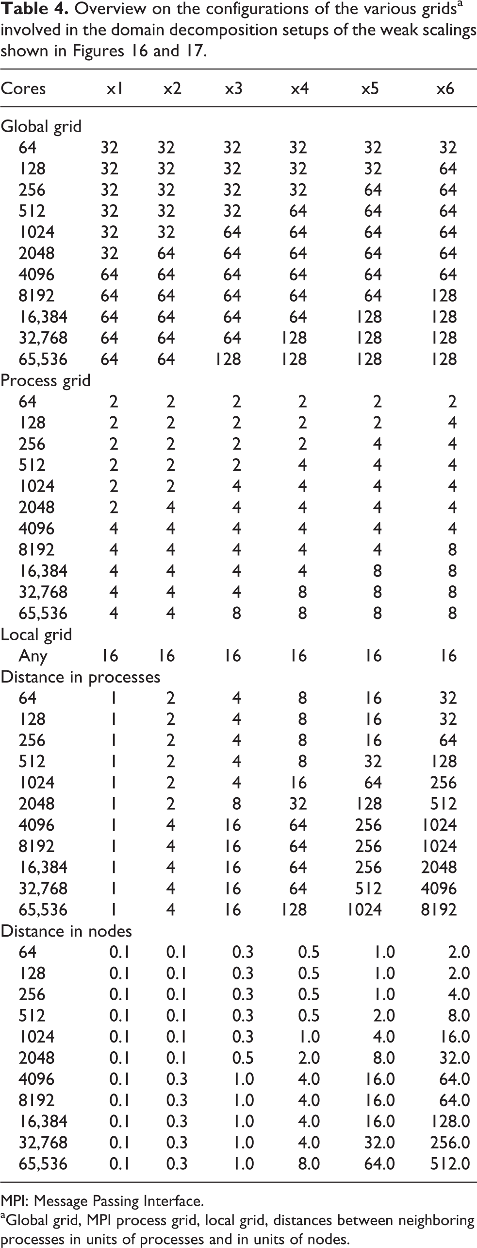
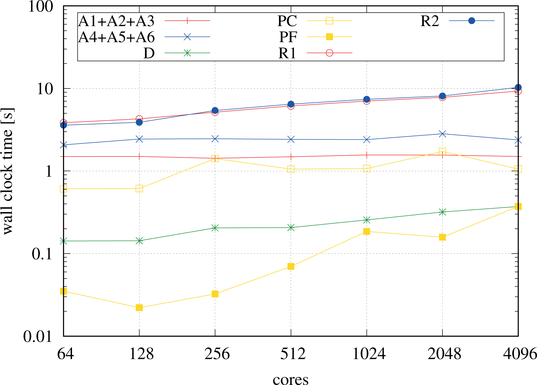
Let us now turn toward an in-depth analysis of the scaling of the building blocks of the domain decomposition code when performing the weak scaling. Figure 17 shows a breakdown of the individual components of the implementation without overlap of communication and computation. Table 4 complements Figure 17 with information on the grid configuration of the runs, essential for a better understanding of the behavior.
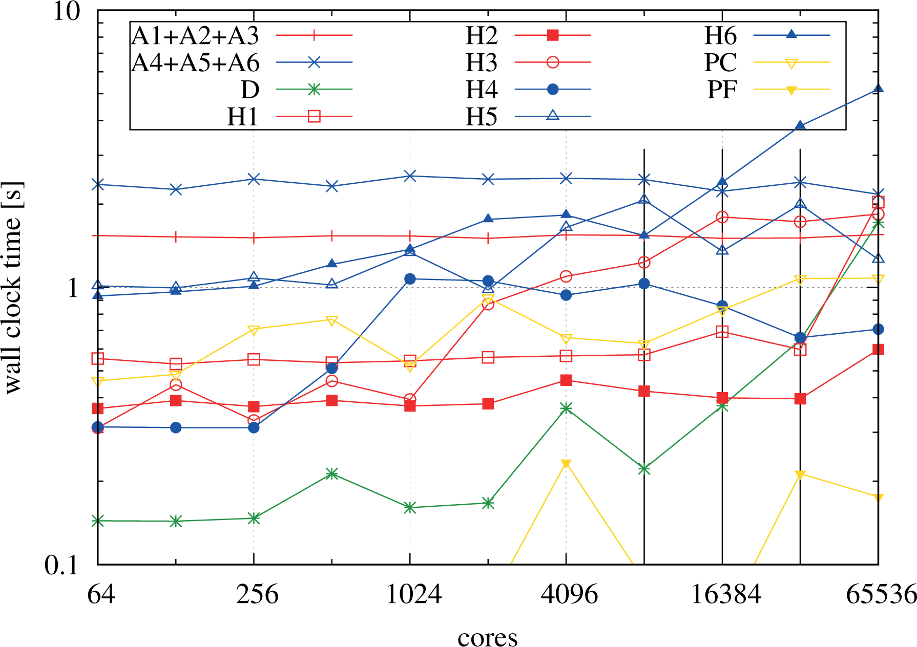
Weak scaling of the building blocks of the implementation for the plain MPI domain decomposition run shown in Figure 16, scanning from 64 up to 65,536 MPI processes. The letter A indicates the advection computations whereas H indicates the halo-exchange operations, for both of which the dimension is given. The letter D represents the diagnostics and P the Poisson solver. In particular, PC means the charge density computation whereas PF means the field solver component, respectively. The X advections and the V advections were grouped together. The transitions going from 1 to 2, from 2 to 4, and from 4 to 8 islands are indicated by vertical lines. MPI: Message Passing Interface.
Overview on the configurations of the various gridsa involved in the domain decomposition setups of the weak scalings shown in Figures 16 and 17.
MPI: Message Passing Interface.
aGlobal grid, MPI process grid, local grid, distances between neighboring processes in units of processes and in units of nodes.
The advection computations (A1–A6) scale virtually ideally. However, from the communication-intensive operations such as the halo exchanges and the Poisson step, we clearly see the effects of the network topology. In the runs performed, the grid of MPI processes is laid out in column-major order, that is, MPI processes are closest in the first dimension and are farthest apart in the sixth dimension, as shown in Table 4 for each problem size of the weak scaling. In particular, the table gives information on how far processes, that are neighbors in the process grid in a logical sense, are separated on the machine in units of processes and nodes, respectively. Note that on the machine and in combination with the configuration we are considering, there are 16 cores (and MPI processes) per node such that any
The communication in
The Poisson step is broken down in two parts, the reduction step (PC) and the actual solution of the Poisson problem (PF). The latter part PF is negligible and scales well (except for some fluctuations especially visible in this step due to the small numbers). The reduction step, on the other hand, shows a similar increase as the
Weak scaling of the building blocks of the implementation for the remap run shown in Fig. 16. The letter A indicates the advection computations whereas R1 and R2 indicate the remap operations involving all-to-all communication, with R1 mapping from the representation contiguous in V to the representation contiguous in X, and R2 inversely. The letter D represents the diagnostics and P the Poisson solver. To improve the clarity of the plot the X advections and the V advections were grouped together.
For comparison, Figure 18 shows the temporal breakdown of the building blocks of the remap code. Starting with four nodes (64 MPI processes) at a resolution of
7.2.3. Intel manycore
Finally, we have also run the same experiment on the Intel KNL partition of the Marconi Fusion cluster at CINECA. We report results from weak scaling starting with a resolution of
Weak scaling on the Marconi KNL partition comparing the domain decomposition codes with and without pipelining, running one MPI process per physical core with four hyperthreads each. MPI: Message Passing Interface.
8. Summary and conclusions
This article addresses the design, implementation, performance optimization, and parallel scalability of a semi-Lagrangian Vlasov–Poisson solver in 6-D phase space. The numerical algorithm is based on dimensional splitting, that is, consecutive interpolation along each of the dimensions. Due to the high dimensionality of the problem, the number of grid points per dimension that can be stored on a compute node is comparably small and significantly limited by memory constraints. For this reason, weak scaling is the most relevant performance metric for this application.
We consider two parallelization schemes, first, a remapping method, and, second, a domain decomposition implementation that parallelizes the grid in all six dimensions, the latter replacing the all-to-all-type of communication of the former with a peer-to-peer (next neighbor) communication pattern. Conventional MPI point-to-point communication is used for the halo exchanges and MPI alltoallv for the remapping, respectively, both in combination with vectorized and OpenMP-based multithreaded interpolation.
We demonstrate by means of extensive performance benchmarks going up to 64 k physical cores that the domain decomposition method shows an excellent weak scaling, only limited by the properties of the network interconnect of the supercomputer, and is superior to the remap scheme with respect to the memory efficiency as well as the parallel performance, despite the fact that the boundary exchange between domains in 6-D is a very communication-intense operation due to dimensionality effects. It is demonstrated that the communication cost can be mitigated by overlapping the computation with communication in a pipelining. We point out that the high efficiency of the hybrid parallelization provides the necessary flexibility to optimally choose the numbers of MPI processes and of OpenMP threads according to the specific architecture of a compute node. This is key for enabling large-scale simulations on modern supercomputers consisting of nodes with ever-growing core counts.
By design, the halo cells used by the domain decomposition introduce restrictions on the time step for the semi-Lagrangian scheme. However, these are mitigated in our implementation using a one-sided blocked communication scheme or a rotating mesh that follows a background magnetic field.
So far, we have only addressed Lagrange interpolation that suits the distributed computations very well due to its locality. In the future, local splines or discontinuous Galerkin interpolation schemes will also be considered. Furthermore, extensions to Vlasov–Maxwell and more complex geometries are natural enhancements. Due to its high efficiency and parallel scalability, the new code enables simulations in 6-D phase space with grid sizes and resolutions large enough for relevant physics cases and paves the way to systematically compare gyrokinetic to fully kinetic simulations.
Footnotes
Acknowledgements
The authors acknowledge discussions with Eric Sonnendrücker. This work has been carried out within the framework of the EUROfusion Consortium and has received funding from the Euratom research and training program 2014–2018. The views and opinions expressed herein do not necessarily reflect those of the European Commission. Parts of the results have been obtained on resources provided by the EUROfusion High Performance Computer (Marconi-Fusion) through the project selavlas. The authors gratefully acknowledge the Gauss Centre for Supercomputing e.V. (www.gauss-centre.eu) for funding this project by providing computing time on the GCS Supercomputer SuperMUC at Leibniz Supercomputing Centre (LRZ, ![]() ) through project id pr53ri.
) through project id pr53ri.
Author contributions
Katharina Kormann and Klaus Reuter contributed equally to this work.
Declaration of Conflicting Interests
The author(s) declared no potential conflicts of interest with respect to the research, authorship, and/or publication of this article.
Funding
The author(s) dislcosed receipt of following financial support for the research, authorship, and/or publication of this article: This work has received funding from the Euratom research and training programme 2014–2018 under grant agreement no. 633053.