Sage Journals: Discover world-class research

Abstract

Running kinetic plasma physics simulations using grid-based solvers is very demanding both in terms of memory as well as computational cost. This is primarily due to the up to six-dimensional phase space and the associated unfavorable scaling of the computational cost as a function of grid spacing (often termed the curse of dimensionality). In this article, we present 4d, 5d, and 6d simulations of the Vlasov–Poisson equation with a split-step semi-Lagrangian discontinuous Galerkin scheme on graphic processing units (GPUs). The local communication pattern of this method allows an efficient implementation on large-scale GPU-based systems and emphasizes the importance of considering algorithmic and high-performance computing aspects in unison. We demonstrate a single node performance above 2 TB/s effective memory bandwidth (on a node with four A100 GPUs) and show excellent scaling (parallel efficiency between 30% and 67%) for up to 1536 A100 GPUs on JUWELS Booster.

Graphical Abstract

Keywords

Fully kinetic simulation general purpose computing on graphic processing units (GPGPUs)Vlasov–Poisson equation semi-Lagrangian discontinuous Galerkin method

Introduction

Computational fluid dynamics has become an extremely successful framework to understand a range of natural phenomena ranging from astrophysics to everyday technological applications. Despite these successes, it is increasingly realized that many phenomena in plasma physics require a kinetic description (Howes et al., (2008); Zweibel and Yamada (2009)). The most challenging aspect of kinetic models, from a computational point of view, is certainly the up to six-dimensional phase space. The traditional approach to overcome this difficulty has been to employ the so-called particle methods (Verboncoeur (2005); Hariri et al. (2016)). While these simulations are comparably cheap and have been successfully employed in some applications, it is well known that they miss or do not resolve accurately certain physical phenomena, such as Landau damping. In addition, the inherent numerical noise introduced makes it extremely difficult to obtain accurate results for many physical phenomena. More recently, sparse grids (Kormann and Sonnendrücker (2016); Guo and Cheng (2016)) and low-rank methods (Einkemmer and Lubich (2018); Einkemmer and Joseph (2021)) have been used to reduce memory requirements and computational complexity. Nevertheless, the need to run fully kinetic simulations in high dimension persists for a range of applications.

To run such simulations, large supercomputers are needed, and codes to facilitate this for CPU-based systems are available. See, for example, Bigot et al. (2013) for a scaling study of the five-dimensional GYSELA code. More recently, also simulations for the full six-dimensional problem have been considered (Kormann et al., 2019). In the latter work, scaling to up to 65,536 processes has been reported on the SuperMUC HPC system of the Leibnitz Supercomputing Center. We also note that the amount of communication required usually increases as we increase the dimensionality of the problem. The reason for this is that the ratio of boundary points (that need to be transferred) to interior grid points increases significantly.

To numerically discretize these models, semi-Lagrangian schemes have proved popular. By using information on the characteristics of the underlying partial differential equations (PDEs), these methods do not suffer from the usual step size restriction of explicit methods. A particular emphasis in collisionless models, as we will consider here, is to introduce as little numerical diffusion as possible into the approximation. It is well known that semi-Lagrangian schemes based on spline interpolation (see, e.g., Sonnendrücker et al. (1999) and Filbet and Sonnendrücker (2003) for a comparison of different methods) and spectral methods (see, e.g., Klimas and Farrell (1994); Klimas and Viñas (2018); Camporeale et al. (2016)) perform well according to this metric.

However, the results for scaling to large supercomputers obtained in Kormann et al. (2019) use Lagrange interpolation instead. The reason for this is that in a massively parallel environment, the global communication patterns induced by spline interpolation or spectral methods provide a significant impediment to scalability. This, in particular, is also a serious issue on GPU-based systems (even on a single node; see, e.g., Einkemmer (2020)). Recently, it has been demonstrated that a different type of semi-Lagrangian scheme, the local semi-Lagrangian discontinuous Galerkin approach, can be implemented efficiently on both Tesla and consumer GPUs, while maintaining or even exceeding the performance of spline-based semi-Lagrangian schemes (Einkemmer 2020).

In this article, we present results, using our SLDG code, that demonstrate that large-scale kinetic simulations of the Vlasov–Poisson equation can be made to scale efficiently on modern GPU-based supercomputers. This is particularly relevant as most (if not all) pre-exascale and exascale systems will make use of GPUs and kinetic simulations are prime candidates that could exploit such systems.

Problem and algorithmic background

Vlasov–Poisson equation

To describe the kinetic dynamics of a plasma, we use the non-dimensionalized Vlasov–Poisson equations:

\partial_{t} f + v \cdot \nabla_{x} f - E (f) \cdot \nabla_{v} f = 0,

(1)

E = - \nabla_{x} ϕ, - Δ ϕ = 1 - ρ, ρ = \int f d v

(2)

where f (t, x, v), with

(x, v) \in R^{d_{x}} \times R^{d_{v}}

, is the (up to) six-dimensional particle density in phase space, ρ(t, x) is the (up to) three-dimensional charge density, and E(t, x) is the (up to) three-dimensional electric field. The Vlasov–Poisson equation is a hyperbolic model that couples a transport equation self-consistently to an equation for the electric field. The electric field is determined via a Poisson problem from the charge density ρ. Since we consider the non-dimensionalized system here, the time is expressed in multiples of the inverse of the plasma frequency.

The particle density is up to six-dimensional. Depending on the physical model, numerical simulations can be run using different numbers of dimensions in space (denoted by d_x) and in velocity (denoted by d_v). In this article, we consider problems with 2x2v (d_x = 2 and d_v = 2, four dimensional), 2x3v (d_x = 2 and d_v = 3, five dimensional), and 3x3v (d_x = 3 and d_v = 3, six dimensional).

While we restrict ourselves to the Vlasov–Poisson model in this work, we emphasize that the performance results obtained provide a good indication for other kinetic models as well. This is true for both problems from plasma physics (such as in case of the Vlasov--Maxwell equations) and kinetic problems in radiative transport.

Time splitting

The first step in our algorithm for solving the Vlasov–Poisson equation is to perform a time splitting. The approach we use here has been introduced in the seminal paper (Cheng and Knorr, 1976) and has subsequently been generalized to, for example, the Vlasov–Poisson equation (Crouseilles et al., 2015).

The idea of the splitting approach is to decompose the nonlinear Vlasov–Poisson equation into a sequence of simpler and linear steps. The strategy to compute the numerical solution at time t ⁿ⁺¹ = t ⁿ + Δt, where we use f ⁿ ≈ f(t ⁿ, x, v), is as follows:

1. Solve ∂_t f (t, x, v) + v ⋅∇_x f (t, x, v) = 0 with initial value f (0, x, v) = fⁿ(x, v) to obtain f ^⋆(x, v) = f (Δt/2, x, v).

2. Compute E using f ^⋆ by solving the Poisson problem (2).

3. Solve ∂_t f (t, x, v) − E(x) ⋅∇_v f (t, x, v) = 0 with initial value f (0, x, v) = f ^⋆(x, v) to obtain f ^⋆⋆(x, v) = f (Δt, x, v).

4. Solve ∂_t f (t, x, v) + v ⋅∇_x f (t, x, v) = 0 with initial value f (0, x, v) = f ^⋆⋆(t, x, v) to obtain f ⁿ⁺¹(x, v) = f (Δt/2, x, v).

This results in a second-order scheme (i.e., Strang splitting). Since the advection speed never depends on the direction of the transport, the characteristics can be determined analytically. For example, for step 1, we have,

f^{⋆} (x, v) = f^{n} (x - v Δ t / 2, v) .

This advection in d_x dimensions can be further reduced to one-dimensional advections by the following splitting procedure

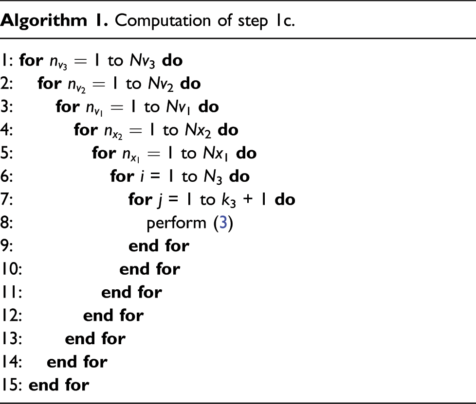
1a. f ^⋆a(x₁, x₂, x₃, v) = f ⁿ(x₁ − v₁Δt/2, x₂, x₃, v).

1b. f ^⋆b(x₁, x₂, x₃, v) = f ^⋆a(x₁, x₂ − v₂Δt/2, x₃, v).

1c. f ^⋆(x₁, x₂, x₃, v) = f ^⋆b(x₁, x₂, x₃ − v₃Δt/2, v).

We emphasize that no error is introduced by this splitting as the corresponding operators commute. We apply a similar procedure to step 3, which results in the following:

3a. f ^⋆a(x, v₁, v₂, v₃) = f ⁿ(x, v₁ + E₁(x)Δt, v₂, v₃).

3b. f ^⋆b(x, v₁, v₂, v₃) = f ^⋆a(x, v₁, v₂ + E₂(x)Δt, v₃).

3c. f ^⋆(x, v₁, v₂, v₃) = f ^⋆b(x, v₁, v₂, v₃ + E₃(x)Δt).

Since the advection in the v-direction (step 3a-3c) does not change the electric field, we have reduced the up to six-dimensional Vlasov–Poisson equation to a sequence of one-dimensional linear advections and a single Poisson solve. The scheme outlined here is second-order accurate (Einkemmer and Ostermann, 2014c). High-order methods have been constructed as well (Casas et al., 2017), and generalization of this basic approach to more complicated problems also exists (see, e.g., Crouseilles et al. (2015) for the Vlasov–Maxwell equations).

The advections are treated using a so-called semi-Lagrangian method, which evaluates the function approximation at the foot of the characteristic curves. Since these end points of the characteristics do not lie on the grid points, an interpolation technique has to be applied. We will describe this procedure in detail in the next section.

Semi-Lagrangian discontinuous Galerkin method

Semi-Lagrangian methods have been widely used to solve the Vlasov equation. In particular, spline interpolation (Sonnendrücker et al. (1999); Filbet et al. (2001)) has emerged as a popular method as it does not introduce too much numerical diffusion, is conservative, and gives good accuracy at a reasonable computational cost.

However, in the construction of a spline, each degree of freedom couples with each other degree of freedom. Due to this global data dependency, spline interpolation is not suited to distributed memory parallelism. To remedy this in Crouseilles et al. (2009), a method that performs spline interpolation on patches has been proposed. However, on today’s massively parallel systems with relatively few degrees of freedom per direction on each MPI process (especially in the six-dimensional case), it is unclear how much advantage this approach provides. In this context, it should be noted that the massively parallel implementation found in Kormann et al. (2019) forgoes using spline interpolation and focuses exclusively on Lagrange interpolation. The same is true for the GPU-based implementation in Mehrenberger et al. (2013). While it is true that Lagrange interpolation scales well, it is also known to be very diffusive and usually large stencils are required in order to obtain accurate results.

In the present work, we will use a semi-Lagrangian discontinuous Galerkin scheme (sldg). This method, see, for example, Crouseilles et al. (2011); Rossmanith and Seal (2011), is conservative by construction (Einkemmer, 2017), has similar or better properties with respect to limiting diffusion than spline interpolation (see Einkemmer (2019) for a comparison), and is completely local (at most two neighboring cells are accessed to update a cell). Thus, it provides a method that in addition to being ideally suited for today’s massively parallel CPU and GPU systems is competitive from a numerical point of view. In addition, a well-developed convergence analysis is available for the Vlasov–Poisson equation (Einkemmer and Ostermann, 2014c,b).

The sldg scheme computes in an efficient way uⁿ⁺¹(y) = uⁿ(y − at). The one-dimensional advections in the previous section are written precisely in this form (all the remaining variables are considered as parameters here). This scheme first divides the domain into cells. The restriction of the solution to each such cell is a polynomial of degree k. Note that there is no continuity constraint across cell interfaces and the approximant is thus discontinuous across this interface (see the left picture in Figure 1). The basis to form these polynomials are Lagrange polynomials which interpolate at the Gauss–Legendre points scaled to each cell. Thus, the degrees of freedom are function values $u_{i j}^{n}$ where the index i is the cell index and the index j refers to the j^th Gauss–Legendre point of cell i. Since the translated function uⁿ⁺¹ in general does not lie in this approximation space, an L² projection is applied, see Figure 1. Only two adjacent cells are required in order to compute the values at a given cell, we denote the index of them with i* and i* + 1. The resulting numerical scheme has order k + 1 and can be written as follows:

u_{i j}^{n + 1} = \sum_{l} A_{j l} u_{i^{*} l}^{n} + \sum_{l} B_{j l} u_{i^{*} + 1; l}^{n}

(3)

Figure 1.

Illustration of the semi-Lagrangian discontinuous Galerkin method. When the advection is complete (central picture), a projection has to be performed which results in the red line in the right picture. This projection lies in the approximation space and is used for subsequent computations. Note that only two adjacent cells are required to compute the values for a certain cell.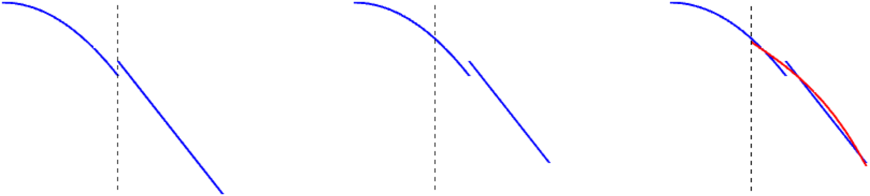

The matrices A and B are of size (k + 1) × (k + 1) and only depend on the advection speed, which can be precomputed. More details about the specific form of these two matrices can be found in Einkemmer (2019).

Poisson solver

To determine the electric field, the Poisson equation (2) has to be solved once in each time step. However, since this is only an up to three-dimensional problem, the computational cost of this part of the algorithm is small. Using FFT-based methods is a common approach that is also supported in our SLDG code.

When the spatial variables x are partitioned over multiple compute nodes, however, the FFT method requires global communication. Thus, we propose an alternative method which requires only local communication to solve this problem. Since the advection is already treated using a discontinuous Galerkin scheme, we will use the same approximation space for the Poisson solver. This has the added benefit that no interpolation to and from the equidistant grid on which FFT-based methods operate is necessary. The details of the discontinuous Galerkin Poisson solver are outlined in the Appendix.

Implementation and parallelization

Our code is written in C++/CUDA and uses templates to treat problems with different numbers of dimensions in physical and velocity space. This allows us to only maintain one codebase, while still providing excellent performance in all these configurations. Our code SLDG is available at https://bitbucket.org/leinkemmer/sldg under the terms of the MIT license.

The main computational effort of the code is due to the following three parts:

Advection: In the advection step, equation (3) is applied to each cell. This is done in a CUDA kernel, and the operation is memory bound on modern GPUs. This step is required whether we run the code on a single GPU or on a large supercomputer, and its cost per degree of freedom is expected to be independent of the number of MPI processes taking part in the simulation.

In 6d, to perform, for example, the advection in direction x₃, algorithm 1 has to be implemented. Nv_1,2,3 and Nx_1,2 are the amounts of degrees of freedom in the corresponding direction, N₃ is the number of cells in direction x₃, and k₃ is the degree of the approximating polynomial. Each thread in the CUDA kernel performs the innermost loop, while the number of threads is given by the second innermost loop. For many problem sizes, this number of threads is too small. Therefore, additional threads work on indices of the third innermost loop. The remaining indices are finally covered by thread blocks.

Algorithm 1. Computation of step 1c.

1: for

n_{v_{3}} = 1

to Nv₃ do

2: for

n_{v_{2}} = 1

to Nv₂ do

3: for

n_{v_{1}} = 1

to Nv₁ do

4: for

n_{x_{2}} = 1

to Nx₂ do

5: for

n_{x_{1}} = 1

to Nx₁ do

6: for i = 1 to N₃ do

7: for j = 1 to k₃ + 1 do

8: perform (3)

9: end for

10: end for

11: end for

12: end for

13: end for

14: end for

15: end for

Communication: In order to run the code on multiple GPUs that possibly span multiple nodes, a domain decomposition approach is used. Depending on the problem, either only the velocity direction or both the space and velocity directions are divided along d_x or d_x + d_v directions. Each of these blocks is assigned to a single GPU. Performing an advection step necessitates the exchange of boundary data from GPU to GPU. On a single node, this can be done using a call to cudaMemcpy, which makes use of NVLink if available. Communication between nodes is done via MPI. Our implementation supports the use of CUDA-Aware MPI which can make use of GPU memory in MPI calls. Thus, in this configuration, MPI routines can directly read from and place data in GPU memory.

Especially for high-dimensional problems, this type of boundary exchange can be relatively expensive. The reason for this is that the number of degrees of freedom in each spatial and velocity direction that can be stored on a single GPU is relatively small (compared to a three-dimensional problem). Thus, boundary cells constitute a larger fraction of the overall degrees of freedom, which due to the discrepancy between GPU memory and InfiniBand bandwidth means that communication can take up a significant fraction of the total run time. The data transfer is illustrated in Figure 2. Let us emphasize, however, that not the entire boundary of each data block associated to a GPU has to be transferred to each neighboring GPU. Since advection is directional, depending on the sign of the velocity field only either a send or a receive is required. This is illustrated in Figure 3. By taking this fact into account, only half the boundary data has to be transferred.

Figure 2.

Illustration of the data transfer between GPUs in the 1+1 dimensional case (i.e., in the x − v plane).The color orange represents the ghost cell data that potentially (depending on the direction of the velocity) has to be sent to neighboring GPUs. Black arrows indicate the corresponding data transfer.

Figure 3.

Demonstration of the advection in the velocity direction and the required boundary data (orange blocks) from neighboring processes. The direction of data transfer depends on the sign of the velocity (the blue function below the illustration).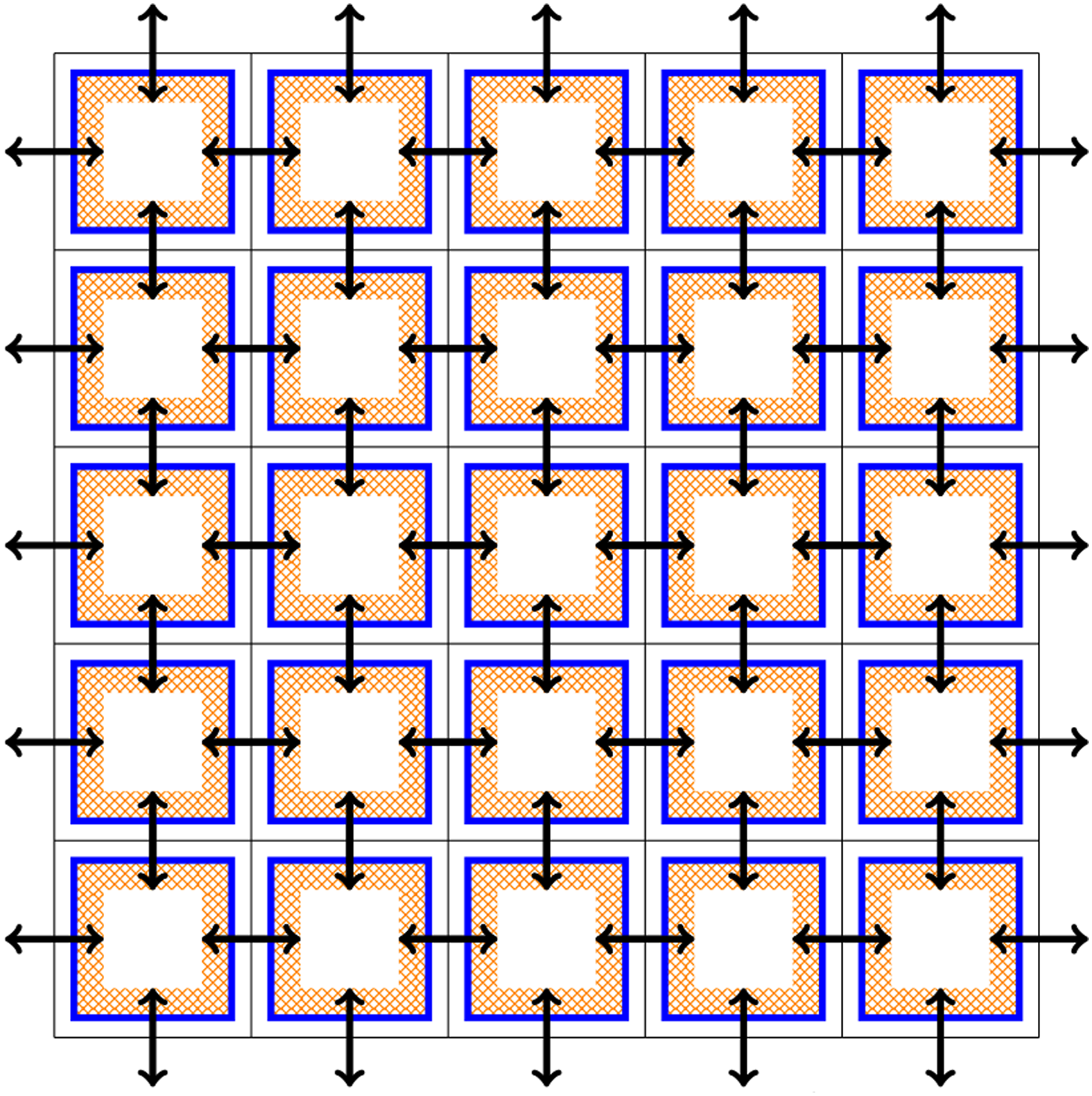

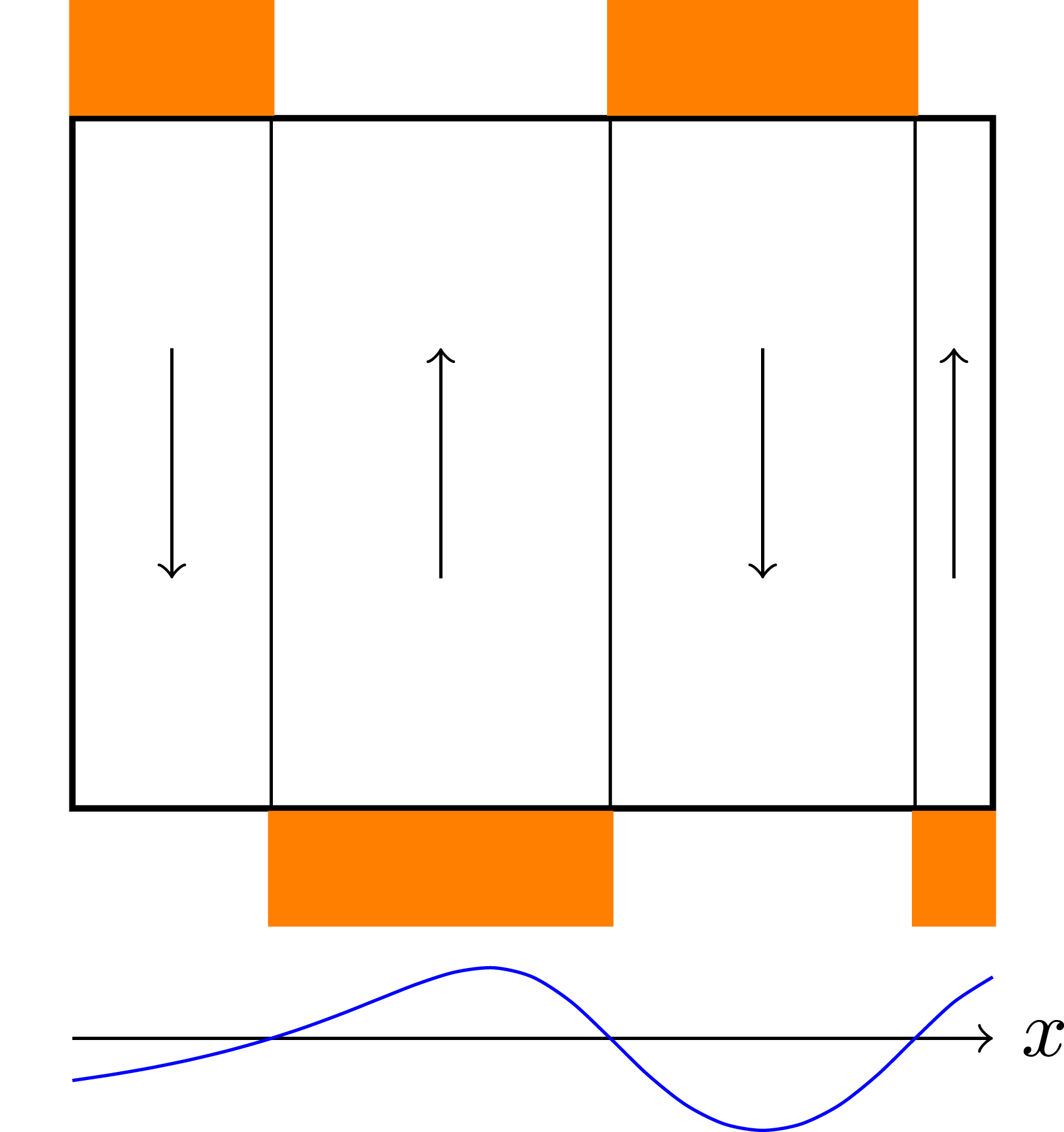
E field: The computation of the electric field proceeds in the following steps. First, the charge density ρ(x) = ∫f (x, v) dv has to be determined. This is first done on each GPU (using the CUB library NVIDIA (2018)), and then a reduction operation in the velocity direction is performed by calling MPI_Reduce on processes which span the entire velocity domain but represent the same part of the spatial domain (as illustrated in Figure 4).

Figure 4.

Illustration of the data transfer necessary to compute the charge density ρ (step 1 in computing the E field).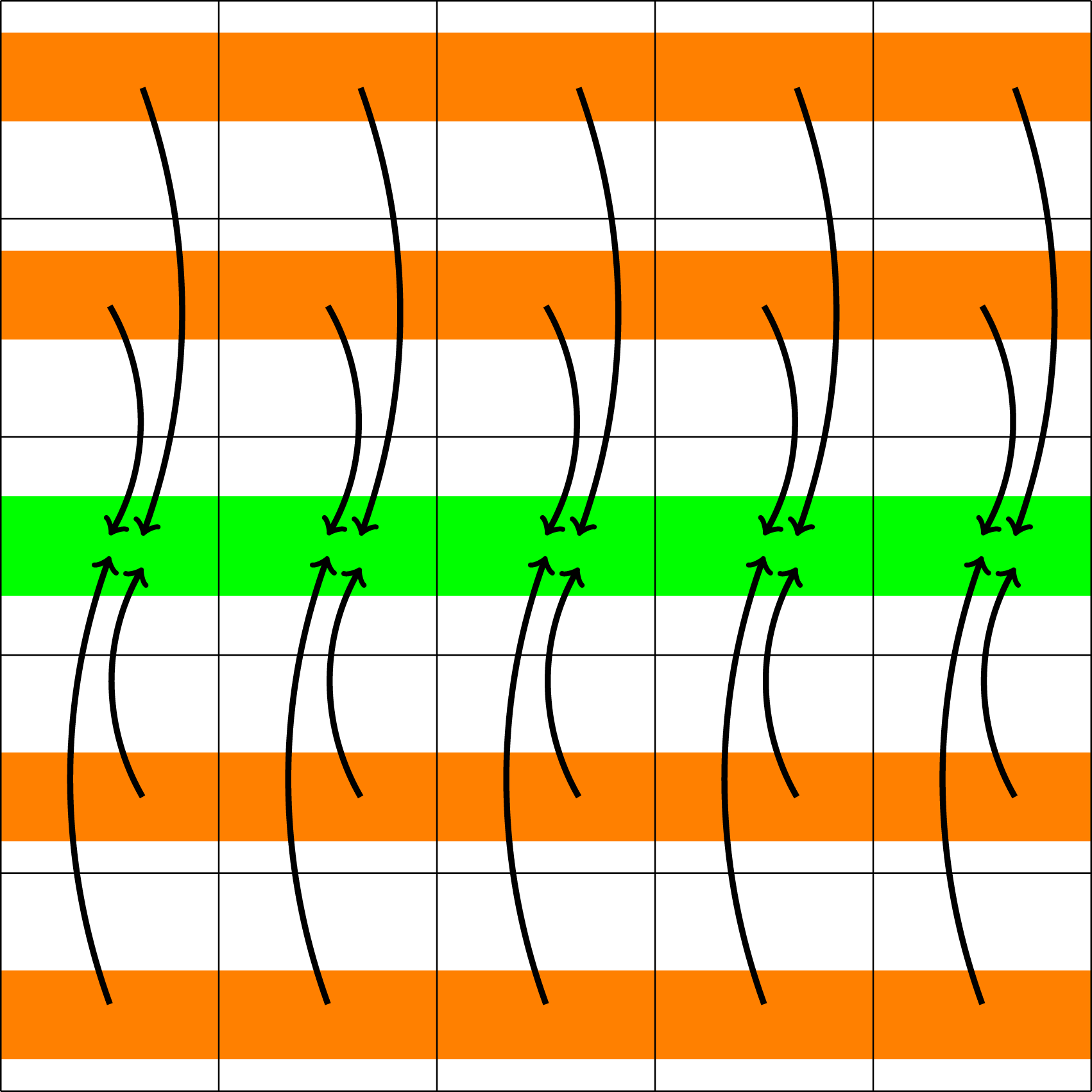

At the completion of this step, ρ is distributed over certain MPI root processes which span the entire space domain. These processes then participate in computing the electric field E. This can be done either by an FFT-based method, which requires global communication among the processes, or an iterative conjugate gradient discontinuous Galerkin (CGdG) solver, which only requires nearest neighbor exchange in each iteration (as illustrated in Figure 5).

Figure 5.

Illustration of the data transfer required to compute the electric field from the charge density ρ (step 2 in computing the E field).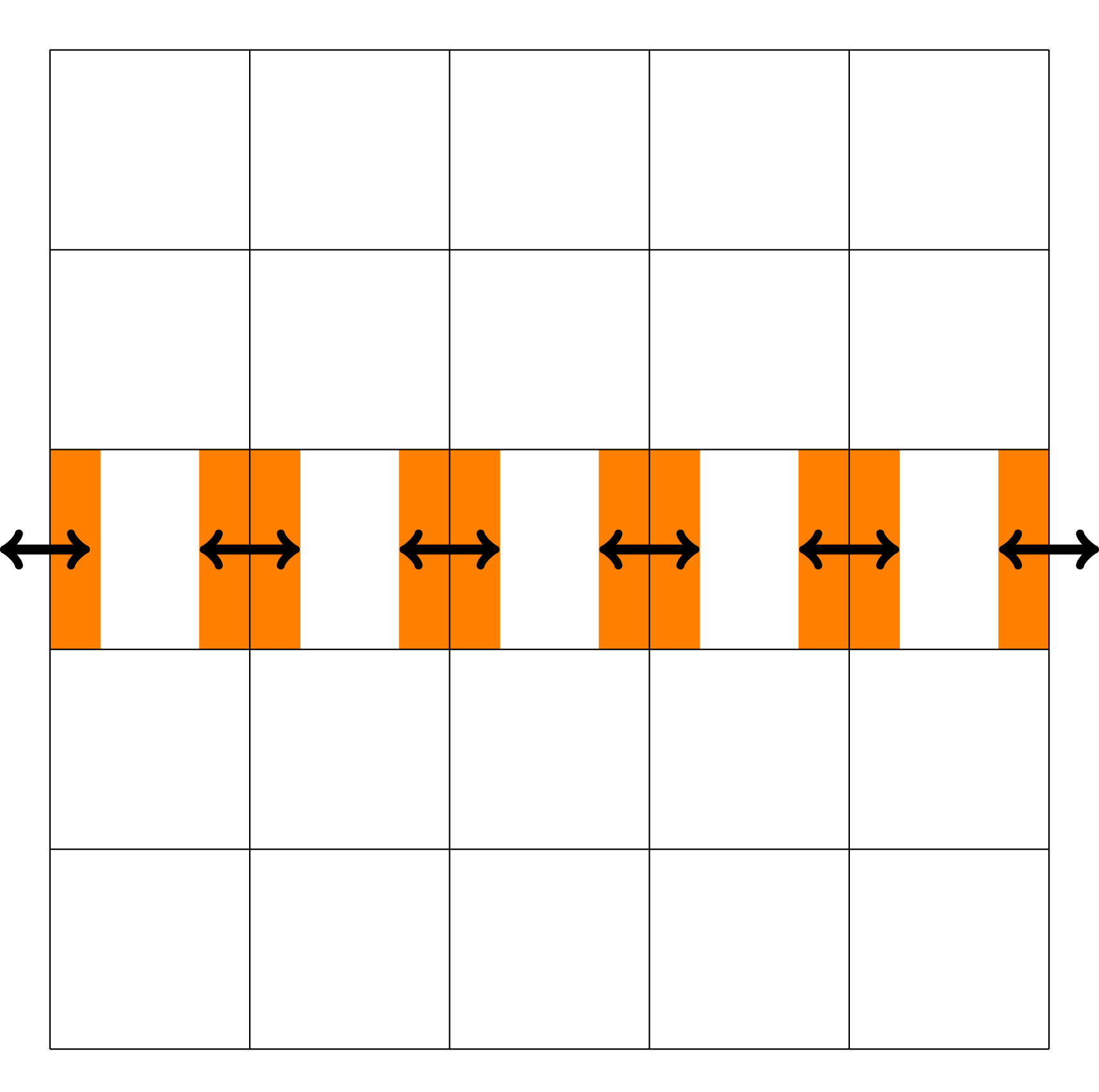

Finally, the electric field has to be made available to all processes that span the velocity domain. To do this, MPI_Broadcast is called (see Figure 6).

Figure 6.

Illustration of the data transfer required to distribute the electric field to the appropriate processes (step 3 in computing the E field).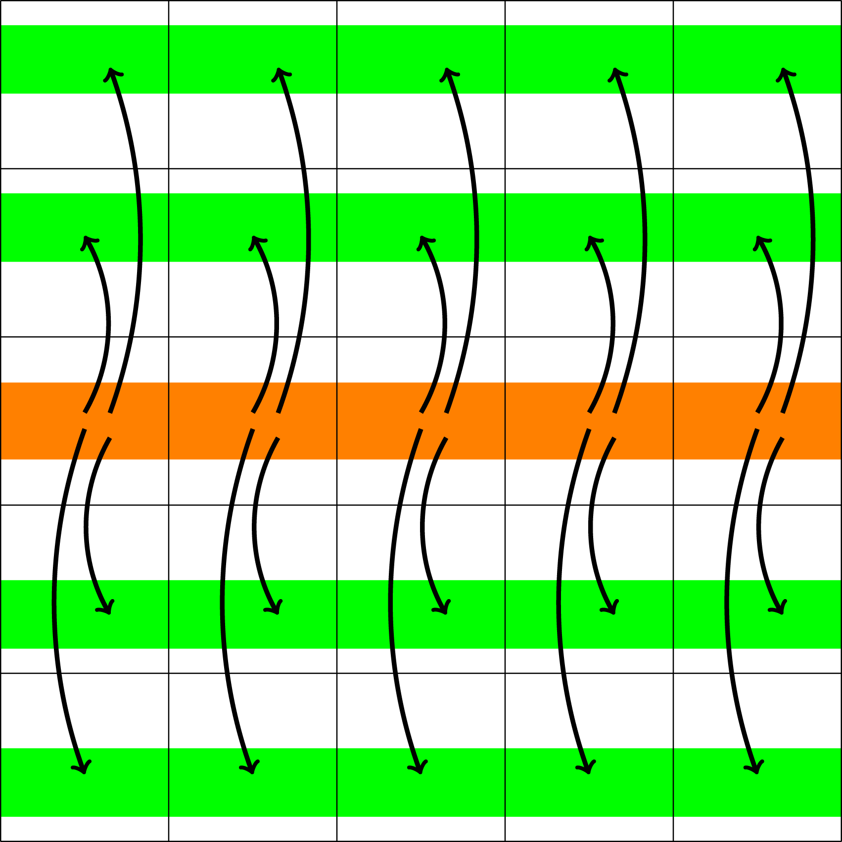

Although from a computational perspective the computation of the electric field is relatively cheap (as it is only an up to three-dimensional problem), the associated data transfer can become an impediment to scaling, especially on large systems.

In a multi-node context, each MPI process is assigned to one or multiple blocks. Each block manages a single GPU. The configuration we employ on most clusters with multiple GPUs on each node is to have one MPI process per node (i.e., one MPI process per shared memory domain) and consequently as many blocks per MPI process as GPUs are on a node. However, on JUWELS Booster, this significantly degrades the bandwidth that is available to conduct MPI communication between different nodes. Thus, the multi-node simulations in this article are run using a single MPI process per GPU. On JUWELS Booster therefore four MPI processes are launched on each node, and CUDA-aware MPI is used both for inter-node as well as intra-node communication.

Validation

To validate our implementation, two commonly used test scenarios are considered. The linear Landau damping problem given by the initial value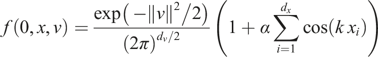

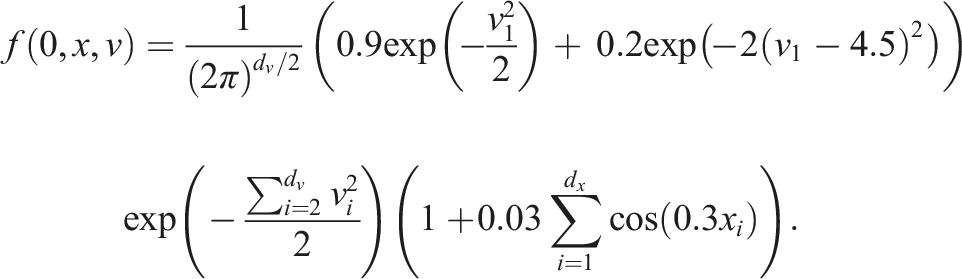
f (0, x, v) = \frac{\exp (- {‖ v ‖}^{2} / 2)}{{(2 π)}^{d_{v} / 2}} (1 + α \sum_{i = 1}^{d_{x}} \cos (k x_{i}))

{[0,4 π]}^{d_{x}} \times {[- 6,6]}^{d_{v}}

, α = 10⁻², and k = 0.5 and a bump-on-tail instability:

\begin{array}{l} f (0, x, v) = \frac{1}{{(2 π)}^{d_{v} / 2}} (0.9 \exp (- \frac{v_{1}^{2}}{2}) + 0.2 \exp (- 2 {(v_{1} - 4.5)}^{2})) \\ \exp (- \frac{\sum_{i = 2}^{d_{v}} v_{i}^{2}}{2}) (1 + 0.03 \sum_{i = 1}^{d_{x}} \cos (0.3 x_{i})) . \end{array}

{[0,20 π / 3]}^{d_{x}} \times {[- 9,9]}^{d_{v}}

In the simulations presented here, we use the 4^th order semi-Lagrangian discontinuous Galerkin scheme (as it represents a good compromise between accuracy and computational cost Einkemmer (2017; 2020)) and a time step size of 0.1. In Figures 7 and 8, the time evolution of the electric energy for these initial conditions is shown for five- and six-dimensional configurations, respectively. The results agree well with what has been reported in the literature. In addition, the Landau damping results show excellent agreement with the analytically obtained decay rate. There is no significant difference between the results obtained with the FFT and discontinuous Galerkin Poisson solver. The SLDG code also includes a set of unit tests that check a range of results against known analytic and numerical solutions and compares the results obtained on the GPU to the results on the CPU.

Figure 7.

Time evolution of the electric energy for the linear Landau damping (top) and bump-on-tail instability (bottom) for the 2x3v case. For both test cases, the 4^th-order method with a time step of 0.1 is used. For the linear Landau test case, 72²144³ degrees of freedom are used (the domain is distributed over eight GPUs), while for the bump-on-tail test scenario 144⁵ degrees of freedom are used (the domain is distributed over 32 GPUs).

Figure 8.

Time evolution of the electric energy of the linear Landau damping (top) and bump-on-tail instability (bottom) for the 3x3v case. For both test cases, the 4^th-order method with a time step size of 0.1 is used. For the linear Landau test case, 36³72³ degrees of freedom are used (the domain is distributed over eight GPUs), while for the bump-on-tail test scenario 72⁶ degrees of freedom are used (the domain is distributed over 64 GPUs).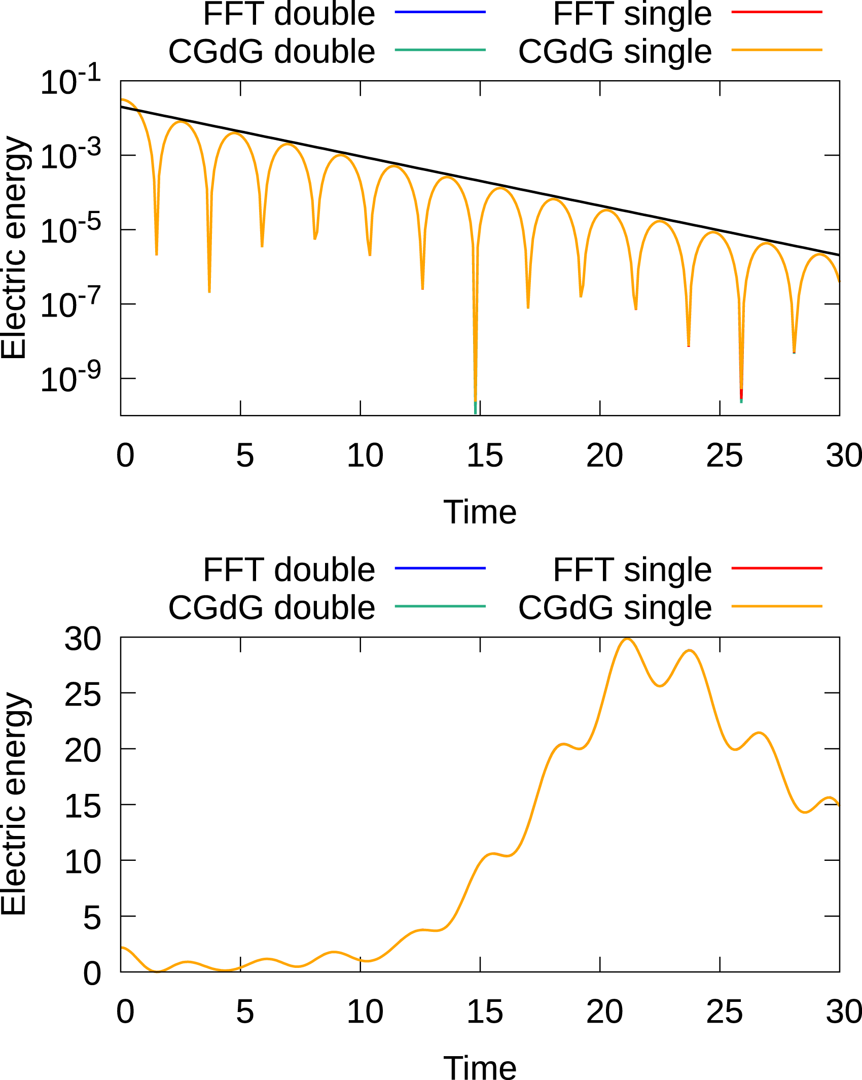

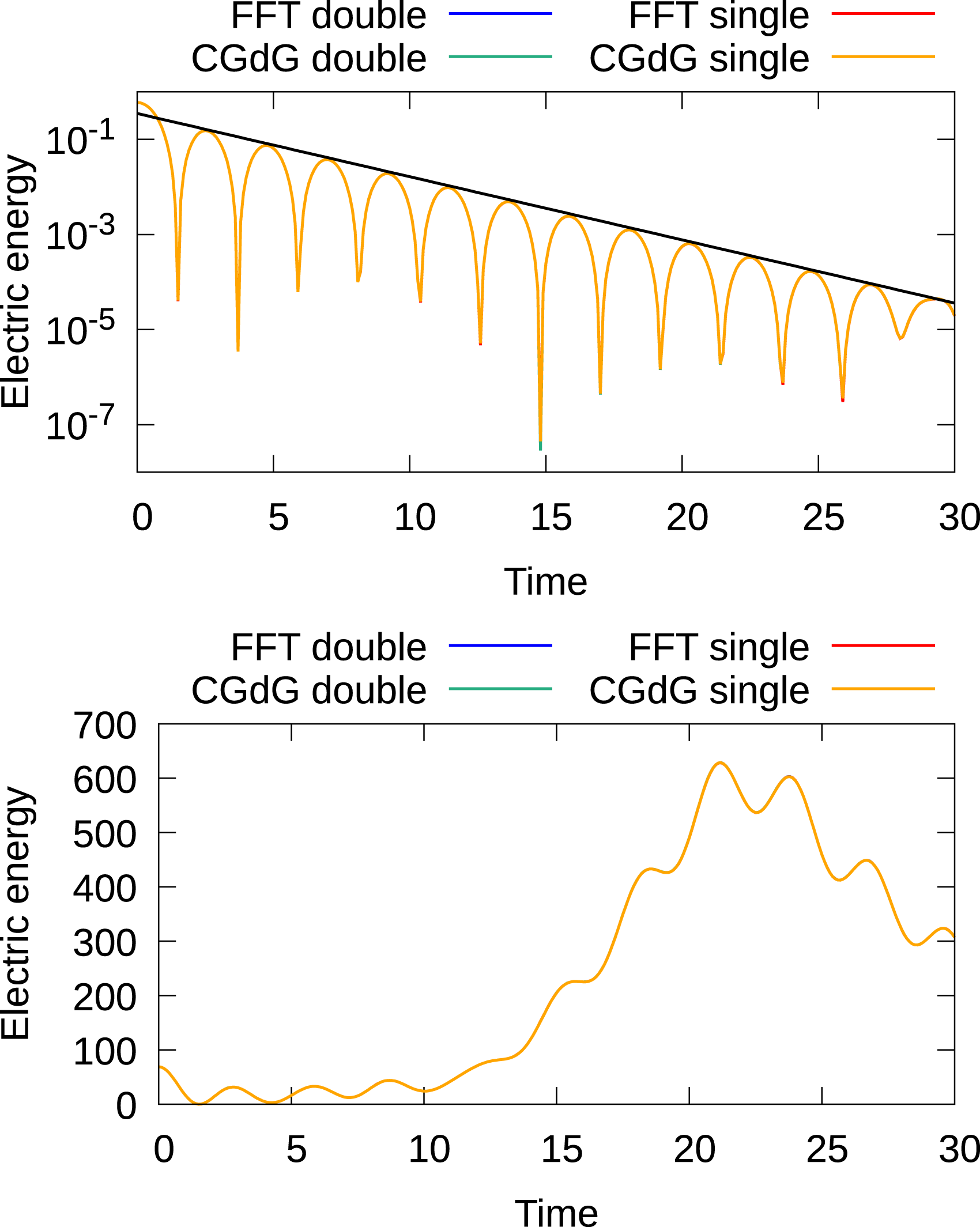
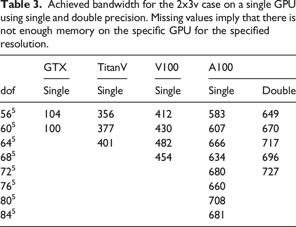
We further remark that the results obtained using single and double precision overlap in the plots. Thus, if one is not interested in too stringent tolerances running simulations with the semi-Lagrangian discontinuous Galerkin scheme in single precision is a viable option. This reduces memory consumption by a factor of two. In particular, for GPUs this can be attractive as memory, in general, is more limited on GPU-based systems. Thus, larger problem sizes can be treated per GPU. In addition, for some problems consumer cards can potentially be used, which do not have strong double-precision performance. We will present and discuss both double- and single-precision results in the remainder of this article.

Single-node performance

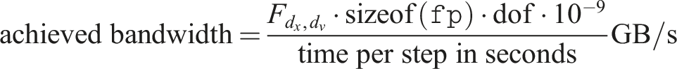
The results in this section are obtained simulating the linear Landau test case. If not otherwise stated, a fixed time step size of 0.1 and the 4th order semi-Lagrangian discontinuous Galerkin method is used. To measure the performance of our code, the achieved memory bandwidth (BW) is used as a metric. This allows us, for our primarily memory bound problem, to easily compare the performance of our implementation with the peak performance of the hardware we run the simulations on. In addition, the run time can be easily obtained from this metric as well.

For the 3x3v (i.e., the six-dimensional) problem solved using the second-order Strang splitting scheme, nine advections have to be performed in each time step. This implies that the entire data have to be accessed 18 times (one read and one write per advection). For the 2x2v and 2x3v problem, six advections have to be performed and the data are consequently accessed 12 times. Moreover, for calculating the electric field once more, the entire data have to be accessed (to compute the density ρ). This is done twice (once at the end of the time step to compute diagnostic values such as the electric energy and once at the middle of the time step). Therefore, we have the following:

achieved bandwidth = \frac{F_{d_{x}, d_{v}} \cdot sizeof (f p) \cdot dof \cdot 10^{- 9}}{time per step in seconds} GB / s

where fp is single or double and

F_{d_{x}, d_{v}}

is 20 for the 3x3v problem and 14 otherwise. For comparison, we give in Table 1 the theoretical peak bandwidth for the different GPUs that we will use in this work. These are the values specified by the vendors and the actual bandwidth obtained, even in a simple benchmark such as copy, is somewhat less.

Table 1.

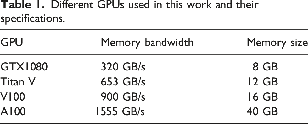
Different GPUs used in this work and their specifications.

GPU	Memory bandwidth	Memory size
GTX1080	320 GB/s	8 GB
Titan V	653 GB/s	12 GB
V100	900 GB/s	16 GB
A100	1555 GB/s	40 GB

Note that the achieved bandwidth is a good measure of performance because the problem is memory bound. To see this, we determine the number of arithmetic operations from equation (3). In total, we require (k + 1)(4(k + 1) − 1) operations per cell. Thus, the flop/byte ratio is as follows: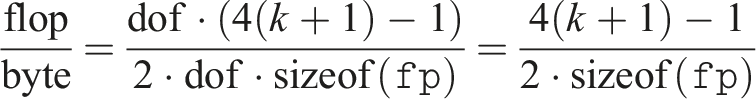

\frac{flop}{byte} = \frac{dof \cdot (4 (k + 1) - 1)}{2 \cdot dof \cdot sizeof (f p)} = \frac{4 (k + 1) - 1}{2 \cdot sizeof (f p)}

For double precision and the 4th-order method, that is, k = 3, this turns out to be approximately equal to 0.94, which is significantly below the hardware flop/byte ratio on modern GPUs (e.g., on A100 the double-precision flop-to-byte ratio is approximately 6.2).

Single GPU performance

First, we compare the performance of the FFT and discontinuous Galerkin Poisson solver. The results are presented in Table 2. The run time for the FFT and the discontinuous Galerkin method is very similar, particular for the 2x3v and 3x3v problems. For the 2x2v problem, the FFT-based scheme is faster by approximately 30%. This can be explained by the fact that the degrees of freedom per direction are reduced for higher dimensional problems (due to computational constraints) and thus not as many iterations are needed to obtain convergence. Since the FFT Poisson solver is faster and there is no disadvantage of using it for single-node computations (we will discuss its role in scaling to larger systems later in this work), all of the computations performed in this section use the FFT-based Poisson solver.

Table 2.

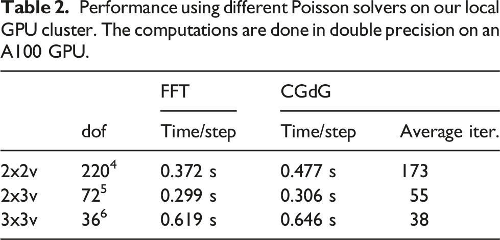
Performance using different Poisson solvers on our local GPU cluster. The computations are done in double precision on an A100 GPU.

		FFT	CGdG
	dof	Time/step	Time/step	Average iter.
2x2v	220⁴	0.372 s	0.477 s	173
2x3v	72⁵	0.299 s	0.306 s	55
3x3v	36⁶	0.619 s	0.646 s	38

In Tables 3 and 4, we show the achieved bandwidth in the 2x3v and the 3x3v cases using four different types of GPUs. We achieve approximately half the bandwidth of what is theoretically possible on each platform. We consider this an excellent result as the memory access pattern is significantly less uniform than in a stencil code and there is a significant amount of computation that is not taken into account by our estimate of the achieved bandwidth (e.g., computing the electric field from the density ρ; see Einkemmer (2020) for a more detailed discussion).

Table 3.

Achieved bandwidth for the 2x3v case on a single GPU using single and double precision. Missing values imply that there is not enough memory on the specific GPU for the specified resolution.

dof	GTX	TitanV	V100	A100
dof	Single	Single	Single	Single	Double
56⁵	104	356	412	583	649
60⁵	100	377	430	607	670
64⁵		401	482	666	717
68⁵			454	634	696
72⁵				680	727
76⁵				660
80⁵				708
84⁵				681

Table 4.

Achieved bandwidth for the 3x3v case on a single GPU using single and double precision. Missing values imply that there is not enough memory on the specific GPU for the specified resolution.

dof	GTX	TitanV	V100	A100
dof	Single	Single	Single	Single	Double
28³28³	64	281	332	415	503
28³32³	66	309	366	462	555
32³32³		355	418	534	590
32³36³			442	554	626
36³36³				460	563
36³40³				482
40³40³				539

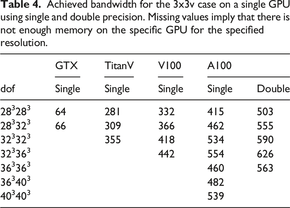
Since single GPU results for the 2x2v and 2x3v cases were already presented in Einkemmer (2020), we will focus on the six-dimensional 3x3v case in the following. In Figure 9, a comparison of the achieved bandwidth between different orders of the method in the 3x3v case is shown. The 4th and 5th order methods achieve better performance than the 2nd and 3rd order methods, which is similar to the behavior observed in Einkemmer (2020) for the 2x2v and 2x3v cases.

Figure 9.

Obtained bandwidth in the 3x3v case as a function of the degrees of freedom where different spatial orders of the method are used. The simulations are done in single precision on an A100 GPU.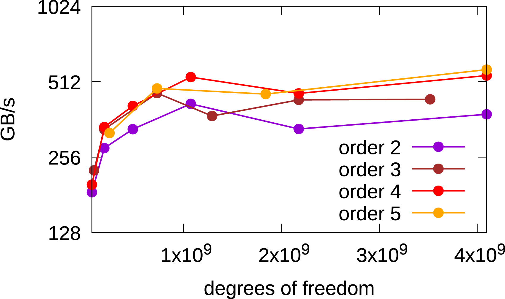

In Figure 10, we show the timings for the different parts that constitute the algorithm in the 2x3v and the 3x3v cases using different GPUs. The chosen number of degrees of freedom is the maximum amount possible on the specific GPU. In the 2x3v case, it can be seen once more that the choice of the Poisson solver has no impact on the overall performance. The main difference between the consumer GPU (the GTX1080) and the enterprise grade GPUs is that the GTX1080 needs more time for the computation of the charge density ρ. This comes from the fact that the GTX1080 is able to perform significantly less floating-point operations per second than the other GPUs. Those are important to compute the diagnostic quantities (such as electric energy) in the reduction step. Similar results can be observed for the 3x3v case.

Figure 10.

Timings for different parts of the algorithm. A single--precision computation with the largest problem that fits into memory for the GPU used has been conducted.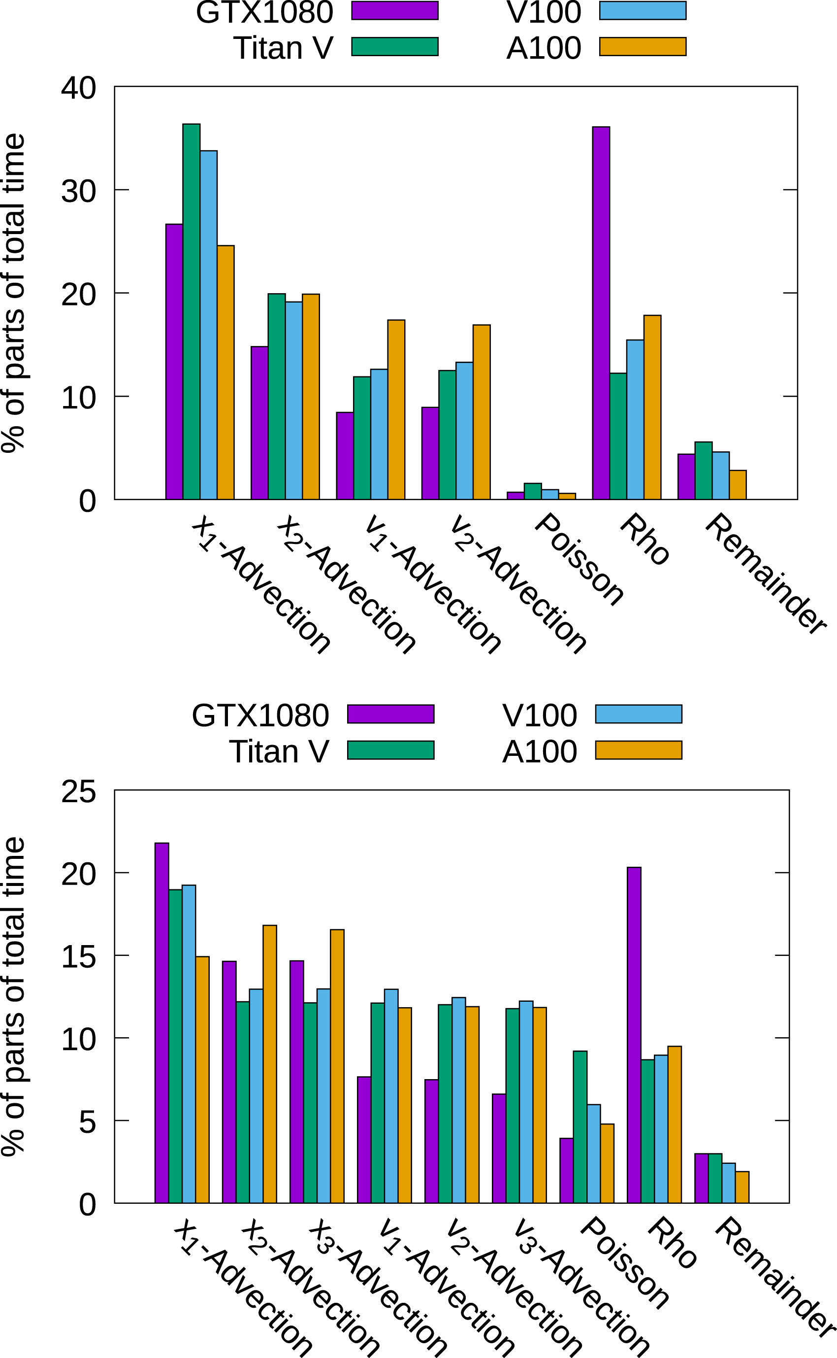

To conclude this section, we will briefly compare the performance between the GPU implementation (which is the focus of the present work) and the CPU implementation. A comparison for the 3x3v problem between the A100 GPU and an Intel Xeon Gold 6226R dual socket system (having 2 × 16 CPUs) is given in Figure 11. It can clearly be observed that the GPU drastically outperforms the CPU-based system. In fact, every part of the code is computed by the GPU in significantly less time. This, in addition to the four and five dimensional results presented in Einkemmer (2020), underscores the advantage of running semi-Lagrangian Vlasov simulations on GPU-based systems. We also note that this is enabled by the semi-Lagrangian discontinuous Galerkin method which, in contrast to spline- or FFT-based interpolation, maps extremely well to the GPU architecture.

Figure 11.

Performance comparison of a CPU-based system and an A100 GPU. The GPU is 24.5 times faster than the CPUs. This comparison is obtained using double precision.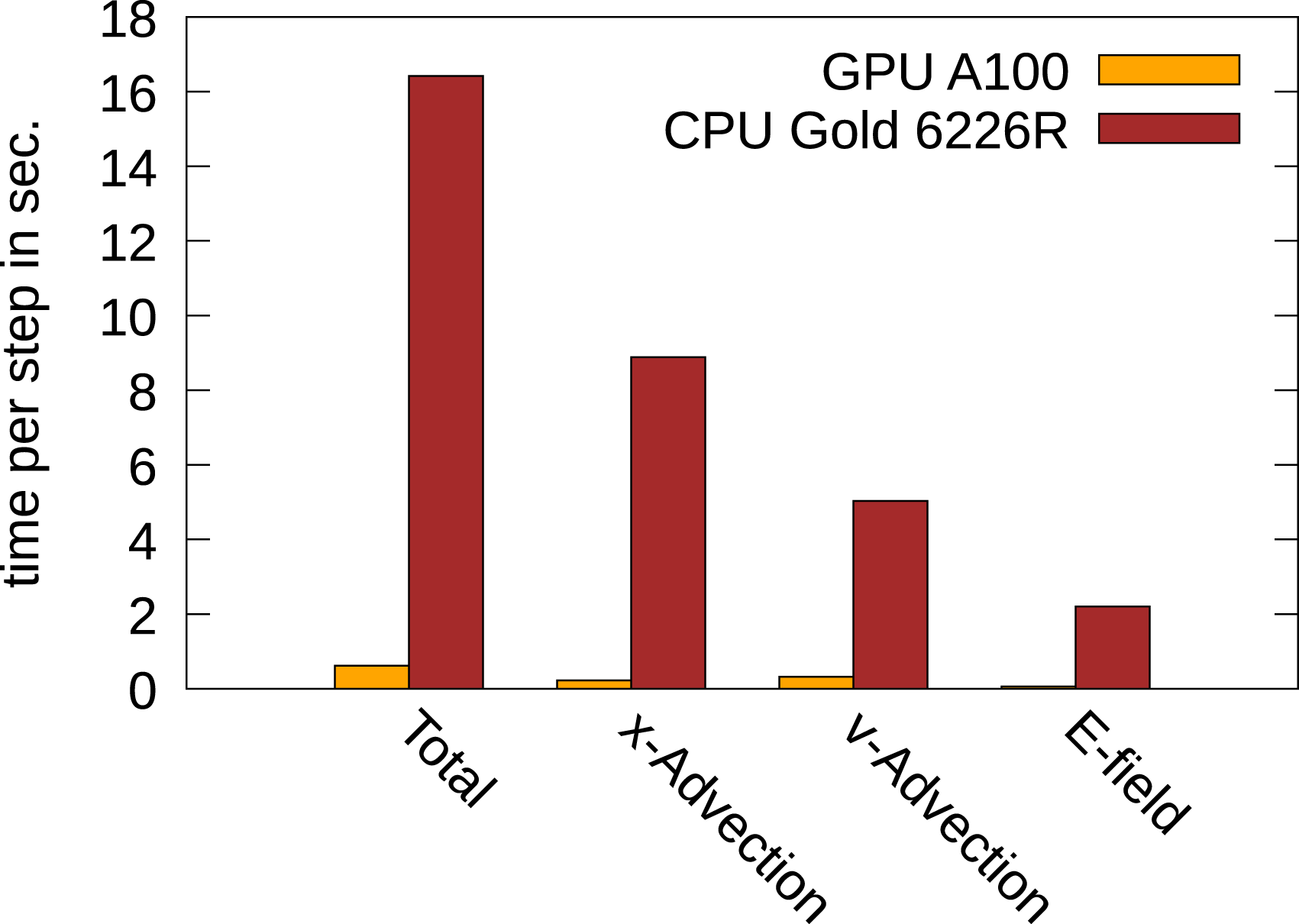

Multiple GPU performance

In this section, we analyze the performance of the code using four A100 GPUs on a single node. We increase the number of grid points in two of the velocity dimensions proportionally to the number of GPUs used. That is, we use weak scaling, which is the only metric of interest for these high-dimensional problems. For the computation, we use the JUWELS Booster supercomputer. The four A100 GPUs on a single node are connected via NVLink3 to each other. The communication process is performed using CUDA-Aware MPI, which automatically uses NVLink for intra-node communication. Since CUDA-Aware MPI is not available on every GPU-equipped system, we also provide an option that uses classic MPI communication between nodes and explicit communication via the host on each node. The corresponding performance results presented in Table 5 have been obtained on JUWELS Booster, where for the without NVLink option the data are explicitly transferred via the host. As we can see, using NVLink results in approximately a factor of 2 improvement, yielding a total single node achieved bandwidth of between 2.05 and 2.55 TB/s.

Table 5.

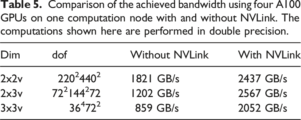
Comparison of the achieved bandwidth using four A100 GPUs on one computation node with and without NVLink. The computations shown here are performed in double precision.

Dim	dof	Without NVLink	With NVLink
2x2v	220²440²	1821 GB/s	2437 GB/s
2x3v	72²144²72	1202 GB/s	2567 GB/s
3x3v	36⁴72²	859 GB/s	2052 GB/s

Scaling to multiple nodes

As can be observed in the previous sections, the resulting grid is still relatively coarse. This is especially true in the five- and six-dimensional cases. In order to run the simulations on finer grids, more nodes are required. In this section, we will report weak scaling results for our code on JUWELS Booster. This is the most important metric for practical applications, where a finer grid is often required in order to obtain physically relevant results. The reported measured wall clock time is the average over the computed time steps. We analyze the total computation time and the time for the pure computation of the advections (denoted as Advection in the figures), the time which is required for the data transfer before the advection takes place (denoted as Communication), and the time for computing the electric field (denoted as E field), which includes the computation of the charge density, the time for solving the Poisson problem (including all the required communication), and the broadcast of the electric field. The time step size is chosen such that the CFL-number is close to one. Moreover, the largest possible local grid which fits into GPU memory is chosen.

2x2v

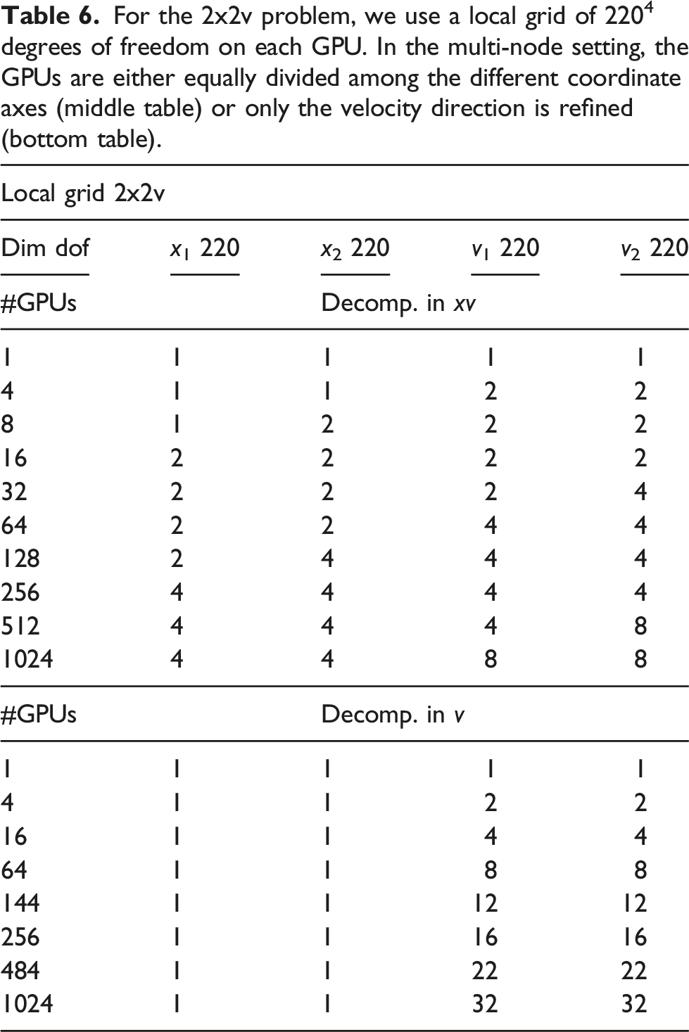
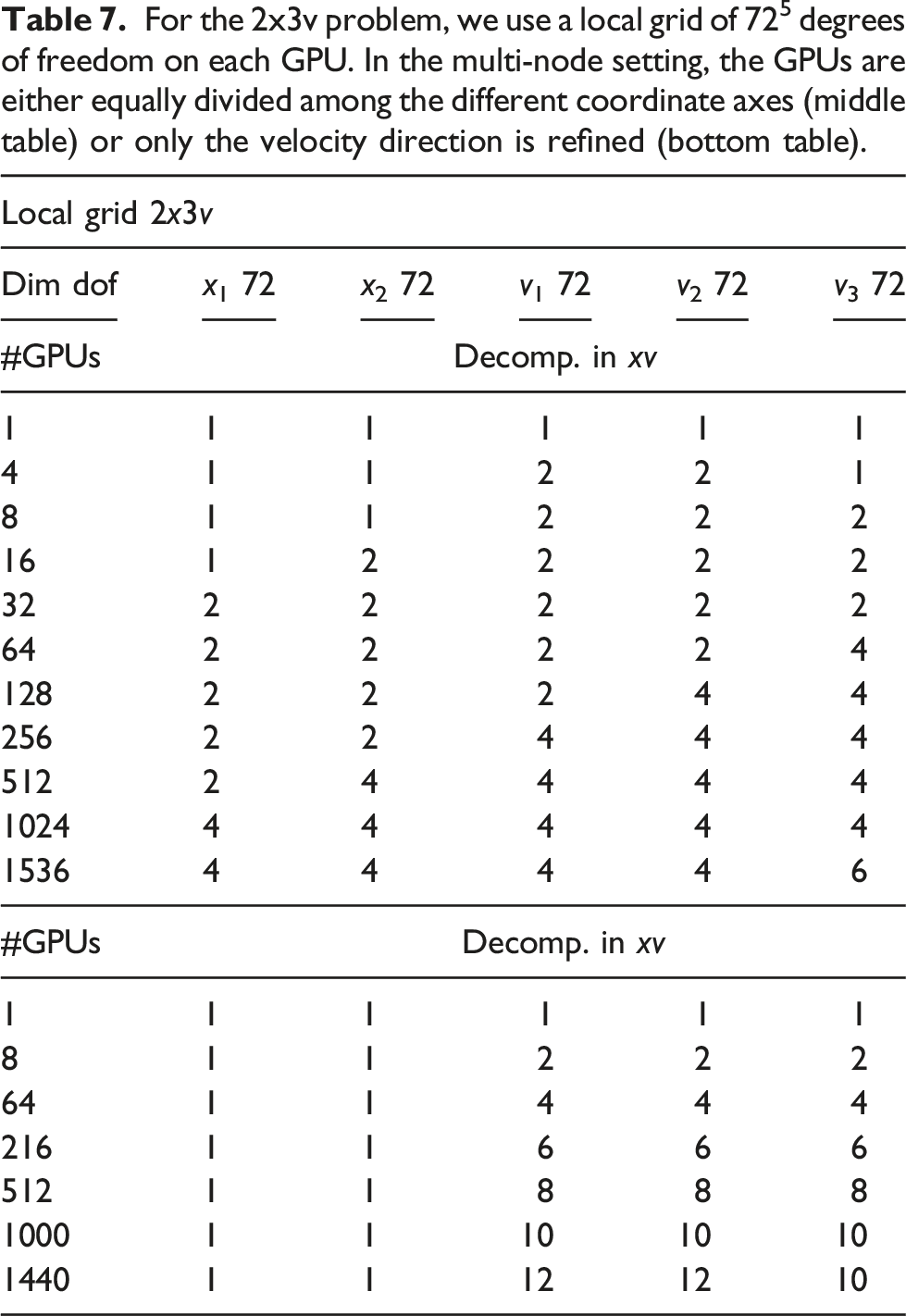
Two test cases are considered in the four-dimensional case. First, the full domain is partitioned and distributed over multiple GPUs, and second, only the velocity domain is refined. The latter is quite common as some problems require a higher resolution in velocity space, for example, to shift back in time the (purely numerical) recurrence effect in linear Landau damping simulations (Einkemmer and Ostermann, 2014a). In Table 6, the considered grids are listed.

Table 6.

For the 2x2v problem, we use a local grid of 220⁴ degrees of freedom on each GPU. In the multi-node setting, the GPUs are either equally divided among the different coordinate axes (middle table) or only the velocity direction is refined (bottom table).

Local grid 2x2v
Dim dof	x₁ 220	x₂ 220	v₁ 220	v₂ 220
#GPUs		Decomp. in xv
1	1	1	1	1
4	1	1	2	2
8	1	2	2	2
16	2	2	2	2
32	2	2	2	4
64	2	2	4	4
128	2	4	4	4
256	4	4	4	4
512	4	4	4	8
1024	4	4	8	8
#GPUs		Decomp. in v
1	1	1	1	1
4	1	1	2	2
16	1	1	4	4
64	1	1	8	8
144	1	1	12	12
256	1	1	16	16
484	1	1	22	22
1024	1	1	32	32

Let us first consider the case when the full domain is distributed over multiple GPUs. The corresponding results are shown in Figure 12. A time step of 0.015 is chosen in order to keep the CFL number below one, and the CGdG method is used to solve the Poisson problem. The largest grid here has 880²1760² degrees of freedom. It can be observed that the time to perform the advection remains constant. This holds for each configuration in this chapter. The communication time in this setting is relatively small as at each time step only 2 GB of data has to be transferred to neighboring MPI processes. The time for computing the electric field increases from 4 to 16 GPUs since a larger problem has to be solved, that is, going from a grid size of 220² to 440² and thus more iterations are required to solve the linear system. The system size stays then constant until 64 GPUs are used. Subsequently, the problem size in physical space increases again. That is, a grid size in the space direction of 880² is used when 256 or more GPUs are used. This again requires more iterations, and the wall clock time increases again. The total time per step rises from about 0.5 seconds to around 1.0 seconds. Thus, running the simulation on 1024 GPUs a parallel efficiency of approximately 50% is achieved.

Figure 12.

Weak scaling in the 2x2v dimensional setting using multiple GPUs for each dimension. A time step size of 0.015 and the CGdG method to solve the Poisson problem are used.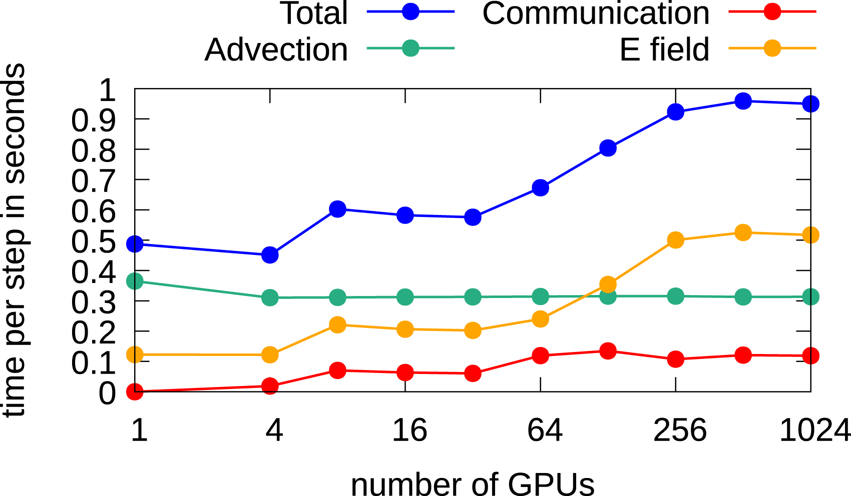

Since the impact of the Poisson solver on the overall performance due to the large number of required iterations in the 2x2v setting is quite high, we also investigate the use of an FFT-based method to solve the Poisson problem. The results are shown in Figure 13. The FFT-based solver is faster on a single node, but scaling is a challenge. Thus, the overall parallel efficiency decreases a little, while overall the run time on 1024 GPUs is still reduced by approximately 10% compared to the CGdG method.

Figure 13.

Weak scaling in the 2x2v dimensional setting using multiple GPUs for each dimension. A time step case size of 0.015 and an FFT-based solver for the Poisson problem are used.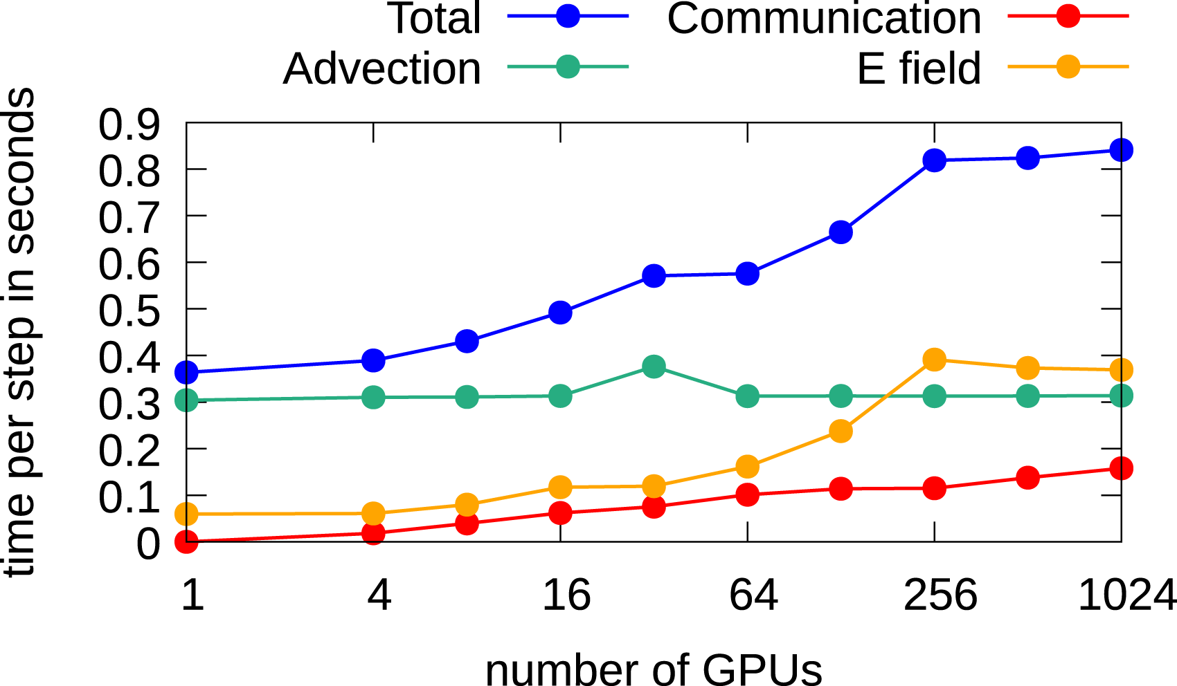

Next, we analyze the behavior when the degrees of freedom are increased in the velocity directions only. Here, since in physical space no parallel numerical method for the computations is required, the FFT-based Poisson solver is used since it is faster. In Figure 14, the weak scaling results are given. It can be observed that the required time for computing the electric field increases when more than 144 GPUs are used. Here, in contrast to the results shown in Figures 12 and 13, not the time for solving the Poisson problem increases, but the required time to compute the charge density increases, that is, the call to MPI_Reduce. The reason for this is that now a very fine resolution of 7040² grid points in the velocity directions is used. The total run time increases from about 0.36 to 0.6; thus, a parallel efficiency of 60% is achieved on 1024 GPUs.

Figure 14.

Weak scaling in the 2x2v dimensional setting using multiple GPUs to increase the degrees of freedom in the velocity dimensions only.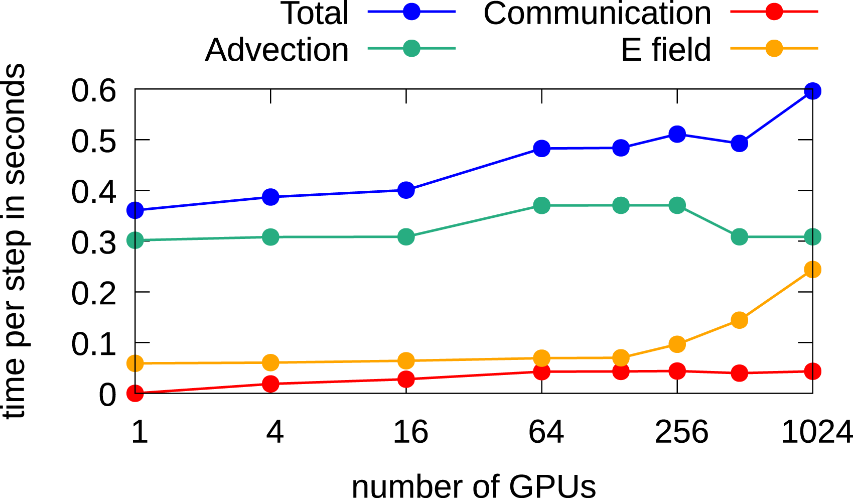

The simulations presented previously were done with a relatively small time step size of 0.015 in order to keep the CFL number in the spatial directions below one. However, the semi-Lagrangian discontinuous Galerkin scheme is also stable for larger time steps. We will thus investigate the parallel efficiency for a CFL number larger than one. The main additional issue here is that the amount of boundary data that needs to be communicated to neighboring processes increases linearly with the CFL number. We use a local grid with a resolution of 216⁴ points and in total 256 GPUs, thus distributing the domain in each direction over four GPUs. The local grid here is slightly smaller than in the previous simulations since additional memory is required to store the boundary data. The CFL number increases from one to five by increasing the time step size by 0.02 until we reach a step size of 0.095 (where the CFL number becomes 5). The results are reported in Figure 15. It can be observed that the time for communication increases continuously, which is expected since more boundary cells have to be sent to the neighboring processes. Furthermore, the time for computing the advection remains almost constant, and the time for computing the electric field increases. This comes from the fact that when solving the Poisson problem iteratively, the starting point is the electric potential obtained at the previous time step. Thus, when a larger time step is used, the initial estimate used in the iterative Poisson solver is farther away from the solution and thus more iterations are required for convergence. Nevertheless, we note that the run for a CFL number smaller than one to a CFL number of five increases by approximately 50%. Thus, running the numerical simulation at a CFL number of five still results in a speedup of approximately a factor 3.3 (despite the increased cost of communication per time step).

Figure 15.

Timings of different parts of the algorithm using CFL numbers larger than one. A local grid of 216⁴ points is used, and the simulation is run on 256 GPUs. We increase the time step from 0.015 (CFL=1) up to 0.095 (CFL=5).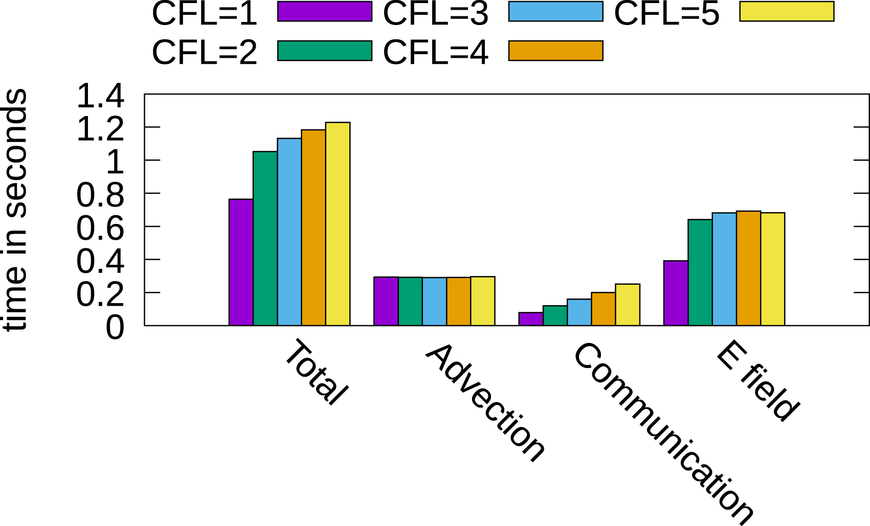

2x3v

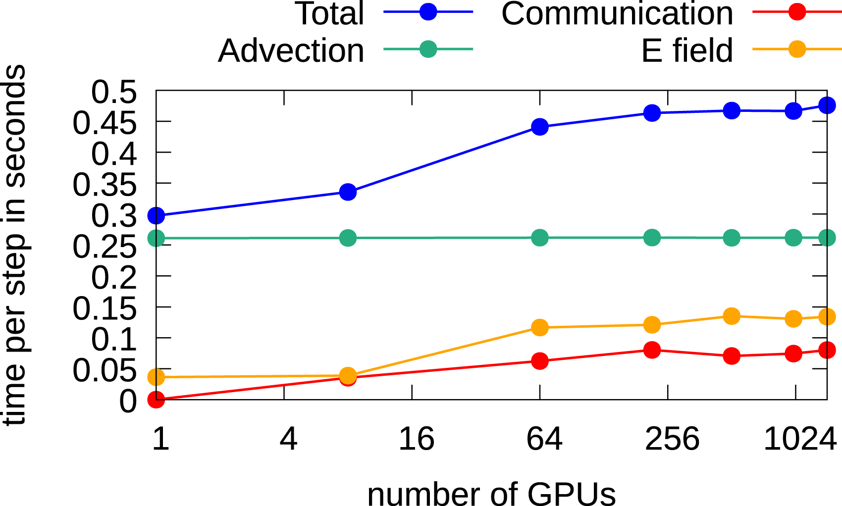
In Figures 16 and 17, the scaling results for the 2x3v case are shown. Again, as in the 2x2v case, two configurations are considered, namely, the full grid refinement and increasing the degrees of freedom in the velocity domain only. The considered configurations are listed in Table 7.

Figure 16.

Weak scaling in the 2x3v case using multiple GPUs for each dimension. A time step size of 0.05 and the CGdG method to solve the Poisson problem are used.

Figure 17.

Weak scaling in the 2x3v dimensional setting using multiple GPUs for velocity dimensions only.

Table 7.

For the 2x3v problem, we use a local grid of 72⁵ degrees of freedom on each GPU. In the multi-node setting, the GPUs are either equally divided among the different coordinate axes (middle table) or only the velocity direction is refined (bottom table).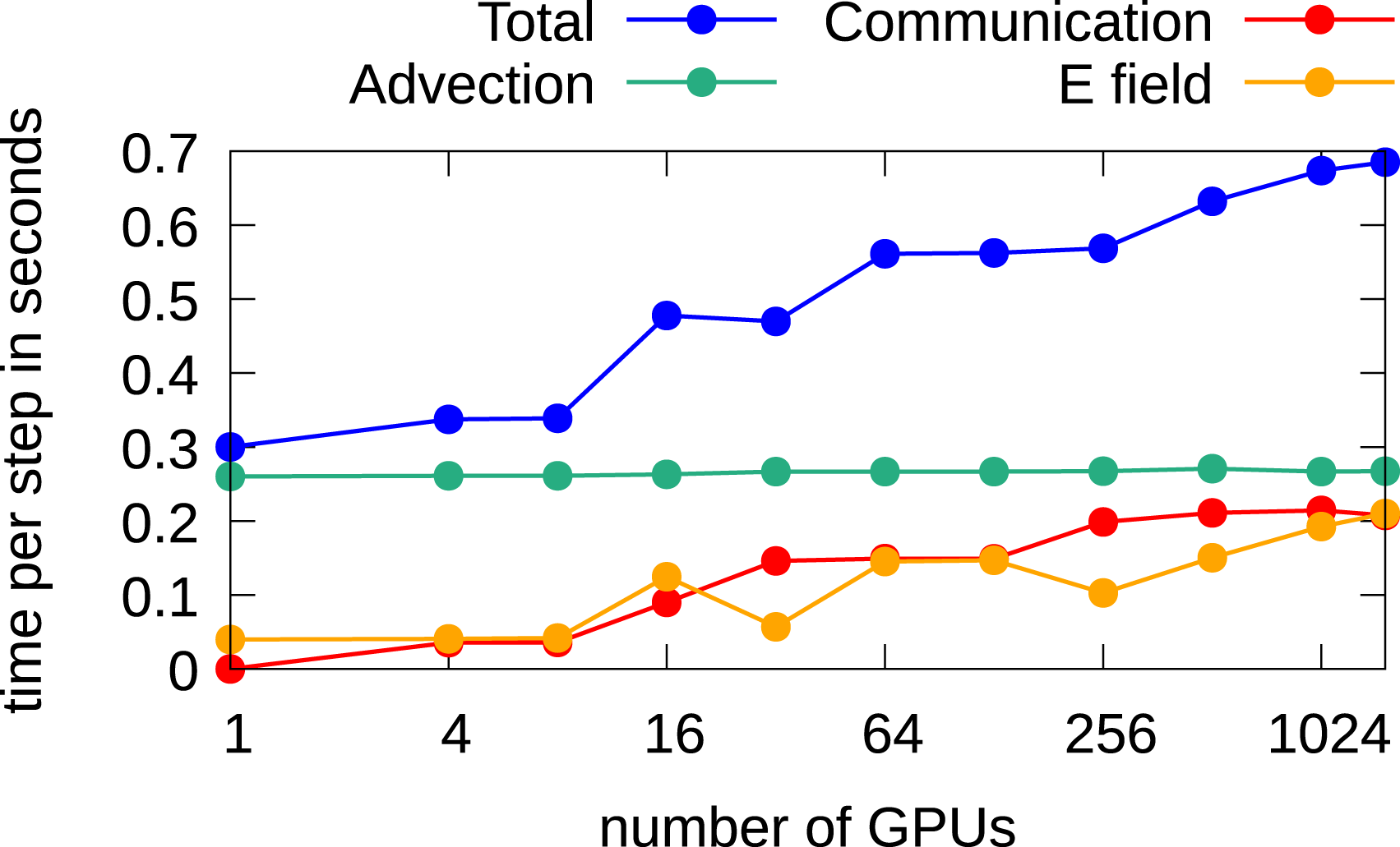

Local grid 2x3v
Dim dof	x₁ 72	x₂ 72	v₁ 72	v₂ 72	v₃ 72
#GPUs		Decomp. in xv
1	1	1	1	1	1
4	1	1	2	2	1
8	1	1	2	2	2
16	1	2	2	2	2
32	2	2	2	2	2
64	2	2	2	2	4
128	2	2	2	4	4
256	2	2	4	4	4
512	2	4	4	4	4
1024	4	4	4	4	4
1536	4	4	4	4	6
#GPUs			Decomp. in xv
1	1	1	1	1	1
8	1	1	2	2	2
64	1	1	4	4	4
216	1	1	6	6	6
512	1	1	8	8	8
1000	1	1	10	10	10
1440	1	1	12	12	10

When the full domain is distributed over multiple GPUs, a time step of 0.05 is chosen which implies a CFL number below one. The CGdG method is used to solve the Poisson problem. The largest problem has a grid of 288⁴432 and is run on 1536 GPUs. In Figure 16, it can be observed that the computation of the electric field has much less impact on the overall performance than in the 2x2v setting. This is mainly because solving the Poisson problem with the CGdG requires less iterations due the smaller number of degrees of freedom per direction. Nevertheless, also here, as expected, an increase of required wall time can be observed if the problem size increases. The time for the communication which is required to perform the advection has more impact on the overall performance than in the 2x2v setting. The CGdG method allows us to limit the impact to performance and is the preferred choice for this five-dimensional problem. For 1536 GPUs, we achieve a parallel efficiency of 43%.

In problems where only additional degrees of freedom are added in the velocity directions, similar results as have been obtained in the 2x2v case can be observed. In this case, the FFT-based solver is the preferred choice. The corresponding weak scaling results are shown in Figure 17, where we observe almost ideal scaling for up to 1440 GPUs. The parallel efficiency in this case is approximately 67%.

3x3v

In the six-dimensional setting, the only reasonable choice is to distribute the problem in each direction (if a distribution is done only in the velocity direction, the number of degrees of freedom in physical space is too small to be of practical interest). The used configurations are listed in Table 8. Using 1536 GPUs results in a grid of size 72¹108¹144⁴ in double precision, which is still relatively coarse, and 80¹120¹160⁴ in single precision.

Table 8.

Configurations in the 3x3v case using multiple GPUs.

Local grid 3x3v double
Dim dof	x₁ 36	x₂ 36	x₃ 36	v₁ 36	v₂ 36	v₃ 36
Local grid 3x3v single
Dim dof	x₁ 40	x₂ 40	x₃ 40	v₁ 40	v₂ 40	v₃ 40
#GPUs			Decomp. in xv
1	1	1	1	1	1	1
4	1	1	1	1	2	2
8	1	1	1	2	2	2
16	1	1	2	2	2	2
32	1	2	2	2	2	2
64	2	2	2	2	2	2
128	2	2	2	2	2	4
256	2	2	2	2	4	4
512	2	2	2	4	4	4
1024	2	2	4	4	4	4
1536	2	3	4	4	4	4

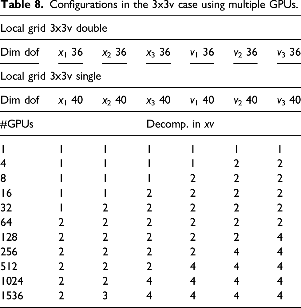
In Figure 18, the scaling results for the 3x3v case are shown. Due to the coarse grid, a time step of 0.1 is chosen which is enough to keep the CFL number below one. The CGdG solver is the preferred choice to solve the Poisson problem. It can be observed that the communication time increases significantly until 64 GPUs are used and remains almost constant afterward. The reason for this behavior is that for a six-dimensional problem, 64 GPUs are required so that in each direction we use more than a single GPU. Due to the nearest neighbor exchange, any further parallelization does, in principle, not contribute to the overall communication time. The time per step increases from 0.6 seconds using one GPU to 1.9 seconds using 1536 GPUs; thus, a parallel efficiency of approximately 30% is achieved.

Figure 18.

Weak scaling in the 3x3v case using multiple GPUs. The spatial configuration is listed in Table 8. Computations are done in double precision.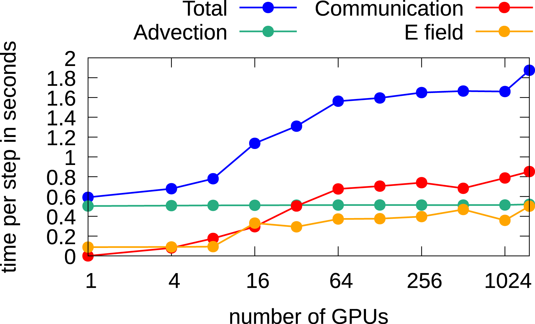

In Figure 19, the results using single precision are shown. Since less memory is required, approximately 1.9 times more degrees of freedom can be considered than double precision. We observe a similar parallel efficiency of approximately 33%.

Figure 19.

Weak scaling in the 3x3v case using multiple GPUs. The configuration is listed in Table 8. Computations are performed in single precision.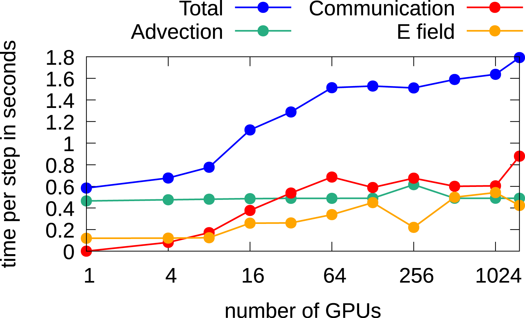

Conclusion

In this work, we have demonstrated that semi-Lagrangian discontinuous Galerkin schemes can be used to run five- and six-dimensional Vlasov simulations on large-scale GPU-equipped supercomputers. The local nature of this method gives excellent performance on a single node using four GPUs (between 2 and 2.5 TB/s depending on the configuration) and scales well to up to 1500 GPUs on JUWELS Booster with a parallel efficiency of between 30% and 67% (depending on the configuration). Since GPU-based supercomputers will play an important role in exascale systems and, most likely, in the future of high-performance computing, the results demonstrated in this work pave the way toward running large-scale Vlasov simulations on such systems.

Footnotes

Acknowledgments

We acknowledge PRACE for awarding us access to JUWELS at GCS@FZJ, Germany. The computational results presented have been achieved in part using the Vienna Scientific Cluster (VSC).

Declaration of conflicting interests

The author(s) declared no potential conflicts of interest with respect to the research, authorship, and/or publication of this article.

Funding

The author(s) disclosed receipt of following financial support for the research, authorship, and/or publication of this article: This project has received funding from the European Union’s Horizon 2020 research and innovation programme under the Marie Skłodowska-Curie grant agreement no 847476. The views and opinions expressed herein do not necessarily reflect those of the European Commission.

ORCID iD

Alexander Moriggl

Discontinuous Galerkin Poisson solver

First, we describe the 1d case which can then be easily extended to arbitrary dimensions, as we will show. The same polynomial space

\begin{array}{c} V_{h}^{k} = { & φ \in L^{2} (Ω) : φ \in P^{k} (I_{i}), \\ I_{i} = [x_{i}, x_{i + 1}], i = 0, \dots, N - 1} \end{array}

that is used to perform the advections is chosen. As basis for

V_{h}^{k}

the Lagrange polynomials interpolating on the k + 1 Gauss–Legendre points x_il restricted to the cell I_i are chosen:

φ_{i j} (x) = {\begin{array}{c} \prod_{l = 0, \dots, k; l \neq j} \frac{x - x_{i l}}{x_{i j} - x_{i l}} & x \in I_{i} \\ 0 & x \in Ω ∖ I_{i} \end{array}

The first step in deriving the discontinuous Galerkin Poisson solver consists in multiplying the Poisson equation (2) by a test function $v \in V_{h}^{k}$ , integrating over each cell I_i = [x_i, x_i+1] and summing up all terms. For more details, see Rivière (2008). This gives, in 1d, the following equation (4)

\begin{array}{l} \sum_{i = 0}^{N - 1} (\int_{I_{i}} ϕ^{'} (x) v^{'} (x) d x - [ϕ^{'} (x_{i})] {v (x_{i})} - \\ {ϕ^{'} (x_{i})} [v (x_{i})] + \frac{σ}{h} [v (x_{n})] [ϕ (x_{n})]) \\ = \int_{Ω} (1 - ρ (x)) v (x) d x, \end{array}

where

{v (x_{i})} = \frac{1}{2} (v (x_{i}^{-}) + v (x_{i}^{+}))

is the average of the function v at the point x_i and

[v (x_{i})] = v (x_{i}^{-}) - v (x_{i}^{+})

is the jump height. From the left hand side of (4) a symmetric bilinear form

a : V_{h}^{k} \times V_{h}^{k} \to R

can be derived. Therefore, we are looking for

ϕ^{DG} \in V_{h}^{k}

such that

a (ϕ^{DG}, v) = l (v) \forall v \in V_{h}^{k}

where the linear form l is defined by the right-hand-side of (4). Plugging

ϕ^{DG} (x) = \sum_{i} \sum_{j = 0}^{k} ϕ (x_{i j}) φ_{i j} (x)

and v = φ_lm into a results in a linear system of the form Au = b where we are looking for the unknown u specified by the coefficients ϕ(x_ij). This method is called the symmetric interior penalty Galerkin (SIPG) method. It can be easily verified that this matrix A is block tridiagonal, and that it can be constructed from two small matrices M and B of size k + 1,

A = \frac{1}{h} (\begin{array}{c} M & B & B^{T} \\ B^{T} & M & B \\ B^{T} & M & B \\ B & B^{T} & M \end{array})

To ensure coercivity of the bilinear form a and positive definiteness of the matrix A, the condition σ ≥ k² is required, see Epshteyn and Rivière (2007). The matrices M and B are defined as follows

\begin{array}{c} {(M)}_{i, j} & = + \frac{1}{2} φ_{j}^{'} (0) φ_{i} (0) + \frac{1}{2} φ_{j} (0) φ_{i}^{'} (0) + σ φ_{j} (0) φ_{i} (0) \\ - \frac{1}{2} φ_{j}^{'} (1) φ_{i} (1) - \frac{1}{2} φ_{j} (1) φ_{i}^{'} (1) + σ φ_{j} (0) φ_{i} (1) \\ + \frac{1}{2} \sum_{l = 0}^{k} φ_{i}^{'} (x_{l}) φ_{j}^{'} (x_{l}) w_{l}, \\ {(B)}_{i, j} & = - \frac{1}{2} φ_{j}^{'} (0) φ_{i} (1) + \frac{1}{2} φ_{j} (0) φ_{i}^{'} (1) - σ φ_{j} (0) φ_{i} (1) \end{array}

where we denote with φ_l (x) the Lagrange polynomials in the interval [0,1] that interpolate the Gauss–Legendre quadrature points x_l. The w_l are the Gaussian quadrature weights. In the higher dimensional setting, the bilinear form is given as follows

\begin{array}{c} a (w, v) & = \sum_{E} \int_{E} \nabla v \cdot \nabla w - \sum_{e} \int_{e} {\nabla v \cdot n_{e}} [w] - \\ \sum_{e} \int_{e} {\nabla w \cdot n_{e}} [v] + \sum_{e} \frac{σ}{| E | / | e |} \int_{e} [v] [w] \end{array}

where E in 2d are rectangles and in 3d are squares, and e are the edges of the rectangles or the faces of the squares. Usually, the denominator in the last term is defined as |e|^β, but setting β = 1 in 2d and

β = \frac{1}{2}

in 3d is almost equivalent if the length of the edges do not vary much. Since in higher dimensions the basis is the tensor product of the 1d basis, the resulting matrix can be written in the following form in 2d

(h_{y} W_{y} \otimes A_{x} + h_{x} A_{y} \otimes W_{x}) u = b

and in 3D

\begin{array}{c} (h_{y} h_{z} W_{z} \otimes W_{y} \otimes A_{x} + h_{x} h_{z} W_{z} \otimes A_{y} \otimes W_{x} + \\ h_{x} h_{y} A_{z} \otimes W_{y} \otimes W_{x}) u = b, \end{array}

where W_x, W_y and W_z are diagonal matrices with the Gaussian quadrature weights on the diagonal.

To solve this linear system at every time step, we are using the conjugate gradient method. The reason why we prefer using this method over a direct method is, that as starting vector of this iterative method the electric potential ϕ computed at the previous time step can be used. Therefore, the number of iterations is small, since, if short time steps are used ϕ does not change dramatically. Moreover, the whole matrix is never constructed, a function is implemented which performs the action of this matrix applied on a vector. Thus, we use a completely matrix-free implementation.

If multiple compute nodes are used, only the boundary cells have to be transferred to the neighboring processes at each iteration. Therefore the method can be parallelized easily. Unfortunately, the matrix is singular since the system does not contain a constraint on the mean value of ϕ. In principle this is not a problem since the electric field is the gradient of the potential function ϕ and therefore this constant shift vanishes. Nevertheless, it is difficult to construct a computationally cheap termination criteria in the CG method when the mean is growing continuously. Therefore, we embedded this condition in the CG method itself with almost no additional computational cost. The resulting CG method, which is mean preserving, is described in Algorithm 2.

Algorithm 2. Mean preserving conjugate gradient method

r₀ = b − Au₀, mean(u₀) = 0

r₀ = r₀ − mean(r₀), p₀ = r₀

$η = {(b + r_{0})}^{T} u_{0}$

while i ≤ MAXITER do

[w_i, mean_w] = Ap_i

$α_{i} = r_{i}^{T} r_{i} / p_{i}^{T} w_{i}$

u_i+1 = u_i + α_ip_i

r_i+1 = r_i − α_i(w_i − mean_w)

$η = η + α_{i} r_{i}^{T} r_{i}$

if ‖r_i+1‖₂ < tol‖b‖₂ then

break

end if

$β_{i} = r_{i + 1}^{T} r_{i + 1} / r_{i}^{T} r_{i}$

p_i+1 = r_i+1 + β_ip_i

end while

To ensure that the dG Poisson solver is working properly, we test it first on a simple example with periodic boundary conditions,

- Δ ϕ (x) = \cos (0.5 x)

In figure 20 we observe that the error is decreasing with order k + 1 (note that the dG Poisson solver converges with the same order as the dG advection solver). Figure 20.

Relative L^∞ error as a function of the number of cells for the discontinuous Galerkin Poisson solver in 2d and 3d. In the Vlasov-Poisson simulations, we set the relative tolerance in the CG method below 10⁻³ which is sufficient as can be seen in Figures 7 and 8. Moreover, σ is set to its minimum allowed value. We observed, that when σ is increasing, also the condition number of the matrix A is increasing and more iterations are required to reach convergence. Additionally, we observe that convergence takes (almost) place within 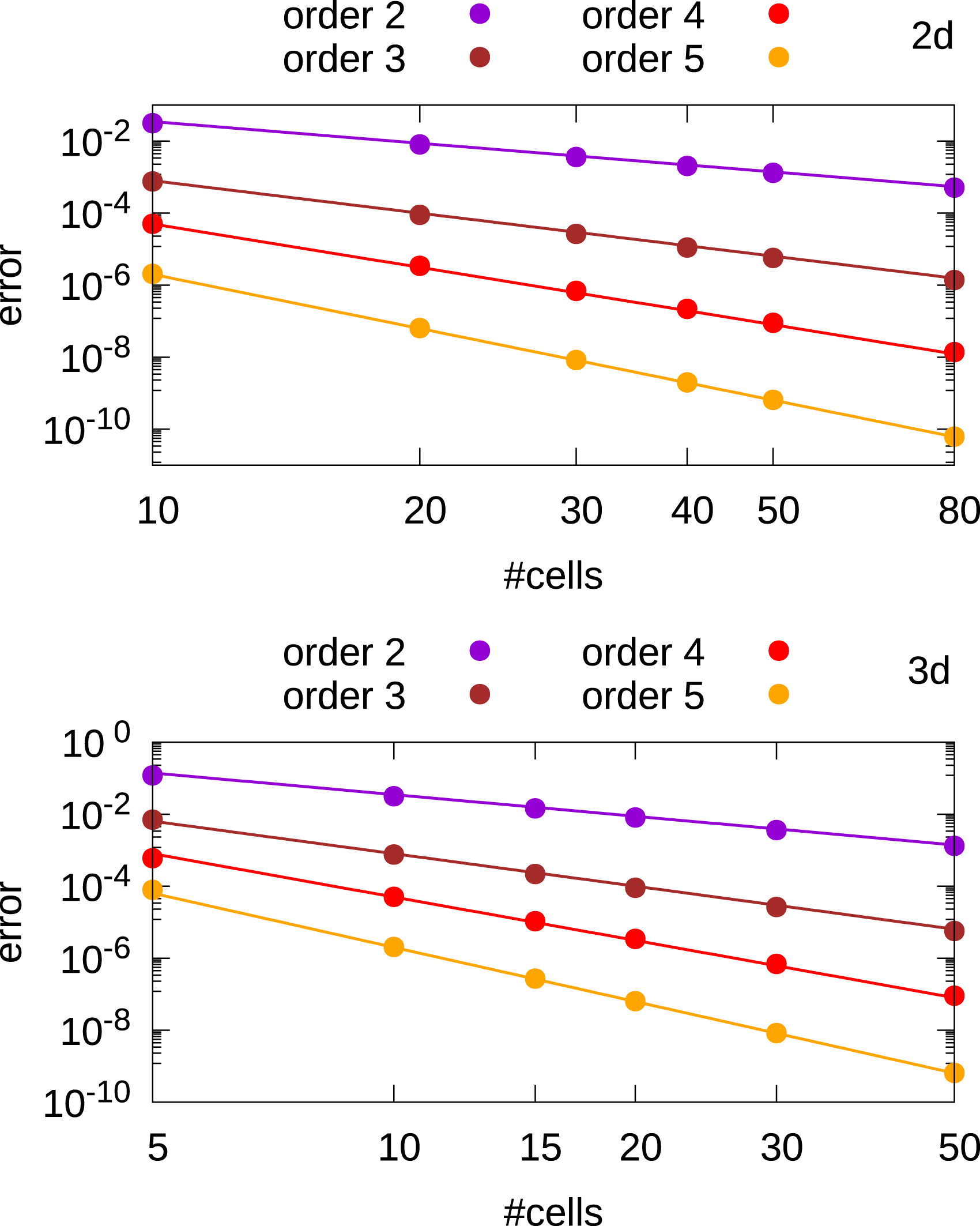$(\prod_{l}^{d x} N_{l} (k_{l} + 1))^{1 / d x}$ iterations. Therefore, we set the maximum number of allowed iterations to this threshold times a safety factor.

Author biographies

Alexander Moriggl received his masters degree in mathematics at the University of Verona. Currently, he is enrolled as a PhD student at the University of Innsbruck. He is working on semi-Lagrangian discontinuous Galerkin methods for GPUs.

Lukas Einkemmer is a professor at the University of Innsbruck. His main research interests include efficiently solving high-dimensional problems in plasma physics and other hyperbolic systems. For example, dynamical low-rank approximation, splitting methods, semi-Lagrangian schemes, and discontinuous Galerkin methods. A particular focus is the development of methods that can be used efficiently on modern computer systems.

References

Bigot

Grandgirard

Latu

, et al. (2013) Scaling gysela code beyond 32K-cores on blue gene/Q. ESAIM: Proceedings EDP Sciences, 43: 117–135.

Camporeale

Delzanno

Bergen

, et al. (2016) On the velocity space discretization for the vlasov–poisson system: comparison between implicit hermite spectral and particle-in-cell methods. Computer Physics Communications 198: 47–58.

Casas

Crouseilles

Faou

, et al. (2017) High-order hamiltonian splitting for the vlasov–poisson equations. Numerische Mathematik 135(3): 769–801.

Cheng

Knorr

(1976) The integration of the vlasov equation in configuration space. Journal of Computational Physics 22(3): 330–351.

Crouseilles

Einkemmer

Faou

(2015) Hamiltonian splitting for the vlasov–maxwell equations. Journal of Computational Physics 283: 224–240.

Crouseilles

Latu

Sonnendrücker

(2009) A parallel vlasov solver based on local cubic spline interpolation on patches. Journal of Computational Physics 228(5): 1429–1446.

Crouseilles

Mehrenberger

Vecil

(2011) Discontinuous galerkin semi-lagrangian method for vlasov-poisson. ESAIM: Proceedings EDP Sciences, 32: 211–230.

Einkemmer

(2017) A study on conserving invariants of the Vlasov equation in semi-Lagrangian computer simulations. Journal of Plasma Physics 83(2).

Einkemmer

(2019) A performance comparison of semi-Lagrangian discontinuous Galerkin and spline based Vlasov solvers in four dimensions. Journal of Computational Physics 376: 937–951.

10.

Einkemmer

(2020) Semi-Lagrangian Vlasov simulation on GPUs. Computer Physics Communications 254: 107351.

11.

Einkemmer

Joseph

(2021) A mass, momentum, and energy conservative dynamical low-rank scheme for the Vlasov equation. Journal of Computational Physics 110495.

12.

Einkemmer

Lubich

(2018) A low-rank projector-splitting integrator for the Vlasov–Poisson equation. SIAM Journal on Scientific Computing 40(5): B1330–B1360.

13.

Einkemmer

Ostermann

(2014a) A strategy to suppress recurrence in grid-based Vlasov solvers. The European Physical Journal D 68: 197.

14.

Einkemmer

Ostermann

(2014b) Convergence analysis of a discontinuous Galerkin/Strang splitting approximation for the Vlasov–Poisson equations. SIAM Journal on Numerical Analysis 52(2): 757–778.

15.

Einkemmer

Ostermann

(2014c) Convergence analysis of Strang splitting for Vlasov-type equations. SIAM Journal on Numerical Analysis 52(1): 140–155.

16.

Epshteyn

Rivière

(2007) Estimation of penalty parameters for symmetric interior penalty Galerkin methods. Journal of Computational and Applied Mathematics 206(2): 843–872.

17.

Filbet

Sonnendrücker

Bertrand

(2001) Conservative numerical schemes for the Vlasov equation. Journal of Computational Physics 172(1): 166–187.

18.

Filbet

Sonnendrücker

(2003) Comparison of Eulerian Vlasov solvers. Computer Physics Communications 150(3): 247–266.

19.

Guo

Cheng

(2016) A sparse grid discontinuous Galerkin method for high-dimensional transport equations and its application to kinetic simulations. SIAM Journal on Scientific Computing 38(6): A3381–A3409.

20.

Hariri

Tran

Jocksch

, et al (2016) A portable platform for accelerated PIC codes and its application to GPUs using OpenACC. Computer Physics Communications 207: 69–82.

21.

Howes

Dorland

Cowley

, et al (2008) Kinetic simulations of magnetized turbulence in astrophysical plasmas. Physical Review Letters 100: 065004.

22.

Klimas

Farrell

(1994) A splitting algorithm for Vlasov simulation with filamentation filtration. Journal of Computational Physics 110(1): 150–163.

23.

Klimas

Viñas

(2018) Absence of recurrence in Fourier–Fourier transformed Vlasov–Poisson simulations. Journal of Plasma Physics 84(4).

24.

Kormann

Reuter

Rampp

(2019) A massively parallel semi-Lagrangian solver for the six-dimensional Vlasov–Poisson equation. The International Journal of High Performance Computing Applications 33(5): 924–947.

25.

Kormann

Sonnendrücker

(2016) Sparse Grids for the Vlasov–Poisson Equation In: Sparse Grids and Applications - Stuttgart 2014. Springer International Publishing, pp. 163–190.

26.

Mehrenberger

Steiner

Marradi

, et al. (2013) Vlasov on GPU (VOG project). ESAIM: Proceedings 43: 37–58.

27.

NVIDIA . (2018) Cub. https://nvlabs.github.io/cub/

28.

Rivière

(2008) Discontinuous galerkin methods for solving elliptic and parabolic equations: theory and implementation. Society for Industrial and Applied Mathematics. DOI: 10.1137/1.9780898717440.

29.

Rossmanith

Seal

(2011) A positivity-preserving high-order semi-lagrangian discontinuous galerkin scheme for the vlasov–poisson equations. Journal of Computational Physics 230(16): 6203–6232.

30.

Sonnendrücker

Roche

Bertrand

, et al. (1999) The semi-lagrangian method for the numerical resolution of the vlasov equation. Journal of Computational Physics 149(2): 201–220.

31.

Verboncoeur

(2005) Particle simulation of plasmas: review and advances. Plasma Physics and Controlled Fusion 47(5A): A231.

32.

Zweibel

Yamada

(2009) Magnetic reconnection in astrophysical and laboratory plasmas. Annual Review of Astronomy and Astrophysics 47: 291–332.

Semi-Lagrangian 4d,5d,and 6d kinetic plasma simulation on large-scale GPU-equipped supercomputers

Abstract

Keywords

Introduction

Problem and algorithmic background

Vlasov–Poisson equation

Time splitting

Semi-Lagrangian discontinuous Galerkin method

Poisson solver

Implementation and parallelization

Validation

Single-node performance

Single GPU performance

Multiple GPU performance

Scaling to multiple nodes

2x2v

2x3v

3x3v

Conclusion

Footnotes

Acknowledgments

Declaration of conflicting interests

Funding

ORCID iD

Discontinuous Galerkin Poisson solver

Author biographies

References