
Abstract
In this article, we compare three data-driven procedures to determine the bunching window in a Monte Carlo simulation of taxable income. Following the standard approach in the empirical bunching literature, we fit a flexible polynomial model to a simulated income distribution, excluding data in a range around a prespecified kink. First, we propose to implement methods for the estimation of structural breaks to determine a bunching regime around the kink. A second procedure is based on Cook’s distances aiming to identify outlier observations. Finally, we apply the iterative counterfactual procedure proposed by Bosch, Dekker, and Strohmaier which evaluates polynomial counterfactual models for all possible bunching windows. While our simulation results show that all three procedures are fairly accurate, the iterative counterfactual procedure is the preferred method to detect the bunching window when no prior information about the true size of the bunching window is available.
Motivation
The bunching approach as introduced by Saez (2010) has been applied to a range of economic problems in recent years (see, among others, Chetty et al. 2011; le Maire and Schjerning 2013; Bastani and Selin 2014; Seim 2017). 1 The methodology exploits the bunching behavior of subjects at kink points of a policy system. For example, kink points in the marginal tax rate or, as in the original paper by Saez (2010), the kink points of the earned income tax credit system are utilized to elicit the elasticity of taxable income (ETI). 2 Due to the convex change in the budget set at the threshold, it is no longer optimal for some individuals—known as the bunching mass—to locate above the threshold. These individuals maximize their utility by moving to the threshold, and hence, an increased mass will be observable at the threshold. The difference between this mass at the threshold and a counterfactual mass derived under the assumption of a smooth budget set is known as the excess mass. The excess mass can then be used to derive, for example, the ETI.
Although the bunching procedure has been acknowledged and replicated in many studies, some authors have found reason to criticize the approach. Einav, Finkelstein, and Schrimpf (2017) show that the bunching pattern can be matched by several alternative economic models, each with a different implication for the counterfactual model. Specifically, the authors find that the frictionless model as assumed in Saez (2010) could lead to elasticities that are up to five times lower than when utilizing a richer dynamic model. This could partially explain the substantial difference between elasticities estimated via the bunching approach and methods that rely on instruments in the spirit of Gruber and Saez (2002), with the latter approach finding larger elasticities. A more fundamental critique with respect to the identification of the ETI is developed separately in Bertanha, McCallum, and Seegert (2019) and Blomquist and Newey (2017), who argue that the structural parameter identified when utilizing the bunching approach can be consistent with any ETI, when the distribution of heterogeneity in preferences is unrestricted. They also argue that the counterfactual distribution utilized in previous studies might not integrate to one, thus preventing it from actually being a distribution. The authors propose to either restrict the distribution of heterogeneity or utilize different budget sets to gain information on the distribution of preferences. An alternative estimator is suggested by Aronsson, Jenderny, and Lanot (2018) to address the same issue. While most studies work within a model framework that avoids making assumptions about the unobservable income component and potential optimization frictions, Aronsson, Jenderny, and Lanot (2018) propose to estimate the ETI with a maximum likelihood estimator based on a log linear labor supply model with log-normally distributed unobserved income component. Although these assumptions can be restrictive, they can in principle be relaxed to capture more general settings allowing the authors to identify the ETI in those cases as well.
The above-mentioned papers criticize the translation of the bunching reaction into the structural parameter ETI, and this discussion is beyond the scope of this article. Here, we focus on a simplified setting and restrict our analysis to smooth counterfactual distributions. However, additional problems exist within the standard bunching framework itself, that is, before the estimate of the excess mass is translated into the ETI. For example, Blomquist and Newey (2017) criticize the dependence on functional form assumptions and Bosch, Dekker, and Strohmaier (2020) argue that relying on eyeballing when determining the counterfactual model should be replaced by a data-driven procedure. We focus on improving the conventional bunching method as such and investigate the performance of different procedures to select the bunching window. We aim to provide recommendations for practitioners how these procedures can be used to make the specification of the counterfactual model less reliant on researchers’ subjective decisions.
Although theoretically all individuals should bunch exactly at the kink point, they face optimization frictions such as adjustment costs and attention costs that prevent them from optimal adjustment. Yearly income is particularly difficult to predict perfectly for some individuals and this difficulty increases with more complicated tax codes. Therefore, empirically, a bunching window of some size around the threshold is observable (Chetty et al. 2011). The bulk of studies implementing the bunching approach relies on eyeballing to determine the bunching window and hedges against any concerns that this might drive results by altering the bunching window in robustness checks. We argue, in the spirit of Bosch, Dekker, and Strohmaier (2020), that the choice of the (only) appropriate bunching window is crucial to the unbiasedness of the bunching estimator and therefore requires a sound data-driven technique to identify it. The bunching window is directly linked to the estimation of the counterfactual model which helps to identify the relative excess mass (b). A bunching window that is too large encompasses individuals that do not bunch and leads to an overestimation of b, irrespective of the location of the kink point in the income distribution. Likewise, a bunching window that is too small leaves out bunching individuals and therefore underestimates the relative excess mass. The imprecision in the measurement of b translates directly into biased estimates of the elasticity.
To circumvent this problem, we discuss two new data-driven procedures and compare them to the data-driven procedure derived in Bosch, Dekker, and Strohmaier (2020). First, we propose to implement methods for the estimation of structural breaks following Bai and Perron (1998, 2003). When moving along the income distribution, the data behave in a certain way, noisy or smooth. At the start of the bunching window however, nonrandom deviations from this behavior can be detected and these form the first structural break in the data. The second structural break is at that point, where the process reverts from the bunching window back to the unaffected region, that is, a smooth income distribution. Thus, two structural break points have to be estimated. A second procedure is based on Cook’s distances that tries to identify influential observations and outliers (Cook 1977). We identify the Cook’s distances—scaled deviations from the least squares projected value—and say that the bunching window is made up of adjacent data points around the threshold that have a significantly positive distance. Third, we apply the iterative counterfactual procedure proposed by Bosch, Dekker, and Strohmaier (2020) which tests all possible combinations of excluded regions within a predetermined interval. The procedure returns a bunching window for each excluded region, from which the mode is taken to determine the bunching window that is to be used for the estimation of the relative excess mass.
We compare these three data-driven procedures to determine the bunching window in a Monte Carlo simulation of taxable income. In contrast to Aronsson, Jenderny, and Lanot (2017) who use a behavioral model to draw data, we use a statistical model to draw simulated data sets which most closely mimic large administrative datasets. Our judgment on the methods is based on two separate questions: First, we compare the three methods with respect to the number of false negatives and false positives they produce. Second, we compare the estimates to a frictionless scenario (i.e., a known bunching “window” located exactly at the kink), where we study the behavior of all three approaches with respect to optimization frictions.
For the baseline specification, we find that the method based on estimation of structural breaks is able to identify most of the bunching individuals. In comparison, the other two procedures perform nearly identically and fail to detect nearly twice the amount of bunching individuals than the procedure by Bai and Perron. We can attribute the superiority of structural break testing methods in this respect to a very conservative estimation of the bunching window. Consequently, the percentage of individuals wrongly attributed as bunching is nearly twice as high as compared to implementing Cook’s distances or the iterative counterfactual procedure. Variations in key parameters reveal a strong sensitivity of the methods for the estimation of structural breaks. Especially when the true bunching window is narrow or very spread out, these methods fail to identify the correct bunching window. The other two procedures are overall more robust and only show sensitivity in the most extreme specifications. Cook’s distances have difficulties determining the true bunching window especially with small sample sizes, large standard deviations, and when the bunching mass is not spread symmetrically around the threshold. Therefore, we find that the procedure by Bosch, Dekker, and Strohmaier (2020) performs best for determining the size of the bunching window although Cook’s distances run it a close second, especially when considering its ease of implementation. Secondary analyses, relating the elasticity estimates to a baseline scenario without optimization frictions, support the finding that the method proposed by Bosch, Dekker, and Strohmaier (2020) is superior in extreme cases.
In the second section, we start by discussing the bunching methodology and highlighting the nature of the problem, before we present our three data-driven procedures that are evaluated in the Monte-Carlo simulations. The simulation design is described in the third section, where we also discuss the outcome measures on which we base our judgement. Fourth section discusses our simulation results and provides an empirical illustration. Fifth section concludes.
Method
Our exposition of the bunching approach closely follows Kleven (2016) to illustrate the main ideas behind the bunching estimator. Although the bunching methodology has been applied in many fields of economics in recent years, its roots lie in the estimation of the ETI, and therefore, we will focus our discussion on this application. However, our results are also relevant for other applications of the bunching approach, such as those discussed in Kleven (2016).
In the ETI case, we consider individuals with preferences defined over after-tax income (value of consumption) and before-tax income (cost of effort). The utility function for those individuals is defined by
if the counterfactual density is constant on the bunching segment
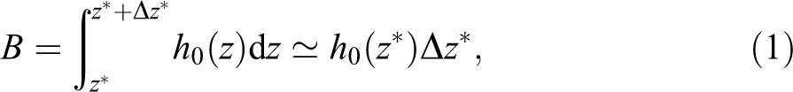
Defining the relative excess mass as
where
More specifically, the counterfactual income distribution around the kink point is estimated employing an auxiliary polynomial regression,
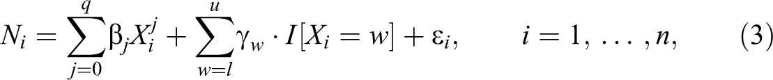
where Ni
denotes the number of individuals in each income bin, Xi
is the midpoint of each income bin, n is the number of income bins, and l and u define the lower and upper bound of the bunching window, respectively. After the order of the polynomial (q) is determined by the Bayesian information criterion (BIC), the predicted values for each income bin are determined using the polynomial coefficients
The outlined strategy is widely applied in the bunching literature (Bastani and Selin 2014; Devereux, Liu, and Loretz 2014; Best and Kleven 2018) but faces some important issues: (i) the true shape of the counterfactual distribution in the bunching segment is unknown and we have to restrict the class of possible distributions to identify the bunching mass, (ii) the identification via polynomial regressions does not ensure that the density predicted by the polynomial regression integrates to one, and (iii) the bunching window is difficult to determine when optimization frictions are present. One the one hand, Bertanha, McCallum, and Seegert (2019) discuss alternative estimation strategies to obtain unbiased estimates of the structural parameter, thereby focusing on the first two issues. On the other hand, Aronsson, Jenderny, and Lanot (2018) choose a parametric approach with explicit distributional assumptions and estimate the ETI with maximum likelihood. Instead, we accept the shortcomings of the polynomial approach and aim to improve the estimation of our polynomial coefficients
Structural Breaks
One way to identify the bunching window is to employ methods from the literature on stability in linear regression models. We assume a smooth population income distribution in the absence of bunching and model the bunching window as a separate regime in which the structure of the distribution changes. We determine the lower bound of the bunching window as a first structural break, or put differently, as the starting point of the second regime. Correspondingly, we determine the upper bound of the bunching window as a second structural break which marks the starting point of the third regime. For this matter, we sequentially add breakpoints to our polynomial regression model using dynamic programming to select the partition of the sample which optimizes the model fit. As these methods were described in several studies by Bai and Perron, we shall henceforth refer to this procedure as BP.
We follow Bai and Perron (1998) and consider a model with a maximum of two breaks and three regimes in which the coefficients remain constant. The regression equation for each regime is then given as
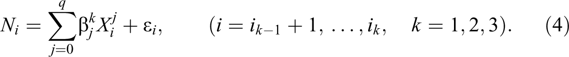
The coefficient estimates are obtained by minimizing the sum of squared residuals for each partition of the income bins with respect to
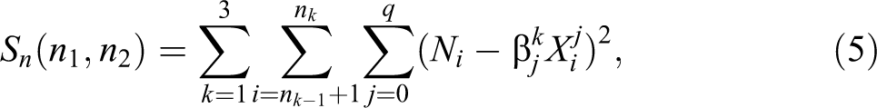
under the assumption that

The optimization is restricted by the requirement that each regime contains sufficient observations so that the coefficients can be identified. The minimum number of observations in each regime is a function of the degree of the polynomial in our application. Bai and Perron (2003) discuss an efficient algorithm to obtain global minimizers of the sum of squared residuals in equation (5). For one threshold in the tax schedule, we specify the maximum number of breaks to be two and expect to find exactly two breakpoints. If the algorithm determines less than two breakpoints, we conclude that the bunching window is not correctly estimated or, put differently, that the algorithm does not detect a substantial bunching mass.
Outlier Detection
Polynomial regressions are generally estimated by least squares. The regression coefficients are chosen so that the sum of squared errors is minimized. Least squares estimation thus tries to avoid large distances between the predicted values and the observed values. Squaring the residuals gives proportionally more weight to extreme points in a sample. Hence, extreme points have a substantial influence on the placement of the polynomial regression curve. The sensitivity of the estimation procedure to extreme observations can be used to detect data points which do not follow the specified model structure, so-called outliers. In the following, we describe how outliers close to the threshold can be identified using Cook’s distances.
Cook (1977) investigates the contribution of data points to the determination of the least squares estimate and proposes to evaluate the Cook’s D statistics
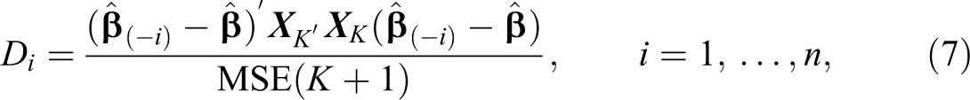
to indicate potentially critical observations.
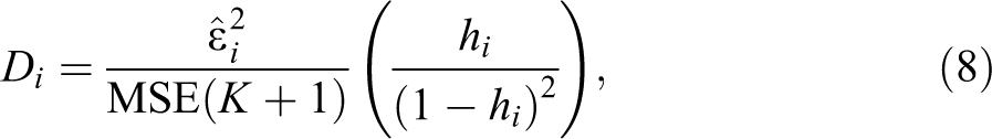
where
In practice, one needs to specify a cut-off value to decide whether observation i is considered an outlier observation. Since
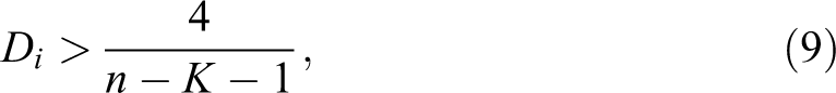
which corresponds roughly to the 1 percent confidence region of the Di statistic. Naturally, the procedure is sensitive to the choice of cut-off value, so that we additionally run simulations with 5 percent and 10 percent confidence regions to check our results for robustness. The Cook’s D is computed for each observation, that is, for each income bin. If we find a set of adjacent observations which are determined to be outliers and if this set includes the threshold, we take those income bins as an estimate for the bunching window.
Iterative Counterfactual Procedure
The iterative counterfactual procedure proposed by Bosch, Dekker, and Strohmaier (2020), henceforth referred to as BDS, tests all different combinations of excluded regions within a predetermined interval. For each excluded region, a polynomial counterfactual model is estimated, which minimizes the BIC while omitting the data points within the excluded region. Based on this counterfactual, those subsequent observations around the threshold that lie outside the 95 percent confidence interval determine the actual bunching window. The procedure returns a bunching window for each excluded region. From this set of bunching windows, the mode is taken to determine the bunching window that is to be used for the estimation of the excess mass (Bosch, Dekker, and Strohmaier 2020).
Formally, the bunching window in Bosch, Dekker, and Strohmaier (2020) is derived as follows: let
where q is chosen as to minimize the BIC. Further, we predict the counterfactual values
We then calculate the upper value of the confidence interval

A positive Ej means that the number of individuals in income bin j exceeds the upper bound of the confidence interval of the predicted number of individuals, as estimated by the polynomial regression. This indicates that more individuals are in the bin than should be in the absence of a kink point. The lower bound of the bunching window, conditional on the respective excluded region, is given by:

which is the smallest adjacent income bin j, starting from the threshold at 0, that still satisfies the condition

which is the largest adjacent income bin j, starting from the threshold at 0, that still satisfies the condition
Simulation Design
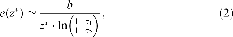
To evaluate the performance of the three procedures, we set up a framework similar to the well-known classification tables, for example used for binary regressions. As outlined before, the bunching window need not be too small nor too large. Hence, a successful procedure needs to minimize misclassifications. On the one hand, our false negatives are made up of those individuals that truly bunch but lie outside the bunching window. On the other hand, our false positives encompass those individuals inside the bunching window that do not belong there because they did not alter their taxable income. Finally, we compute the elasticity parameter according to equation (2) and investigate how a wrongly specified bunching window affects the bunching estimator. Since the restrictive assumptions of the polynomial strategy are violated in some specifications of our data-generating process, we expect the bunching estimator to be biased in those cases and additionally study the relative bias compared to situations without optimization frictions to distinguish between both sources of bias.
In each iteration, we draw from a log-normal distribution of potential incomes,
6
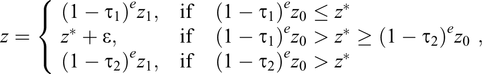
where
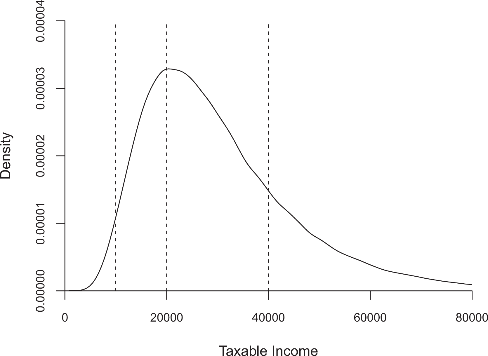
Log-normal distribution of before-tax incomes with kink point locations (vertical dashed lines).
Because the analyzed procedures are data-driven, the sample size should play a role in determining the appropriate bunching window. Likewise, the choice of binwidth and the location of the kink point determine the shape of the section from the income distribution under consideration, which could influence the ability of the data-driven procedures to determine the correct bunching window. Since the majority of papers (e.g., Chetty et al. 2011; Bastani and Selin 2014; Seim 2017) focus on top incomes, we chose
Results
Monte Carlo Simulation
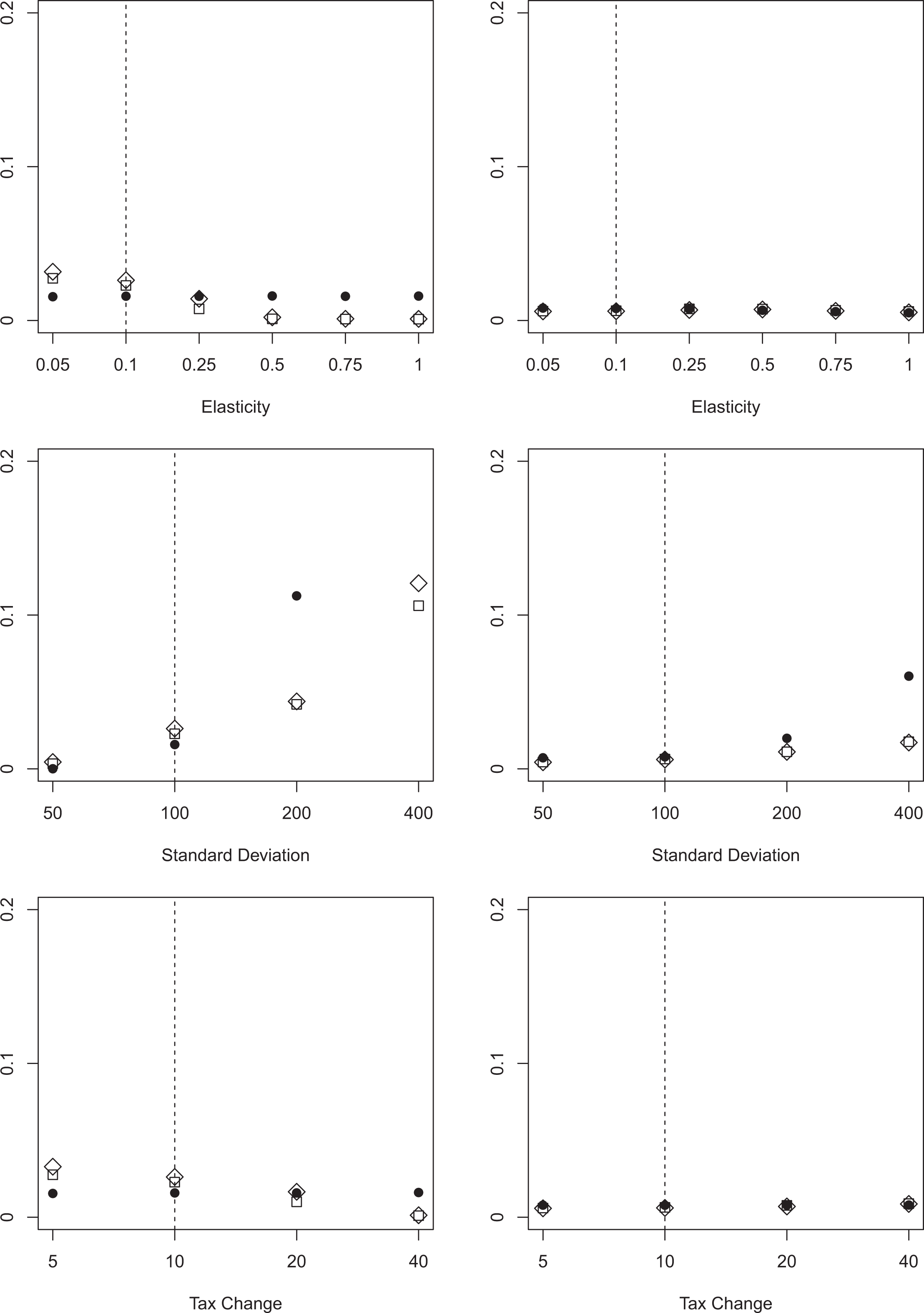
In the first set of specifications, the error term follows a normal distribution which is symmetric around the mean. We consider different configurations of all key parameters of the baseline specification. To account for the possibility of asymmetric bunching windows, we alter the structure of the error term in such a way that we obtain a left-skewed and a right-skewed distribution in later specifications. The results for the false negatives simulations for the normally distributed error term are depicted in figure 2. We report the average percentage of false negatives over 1,000 replications.
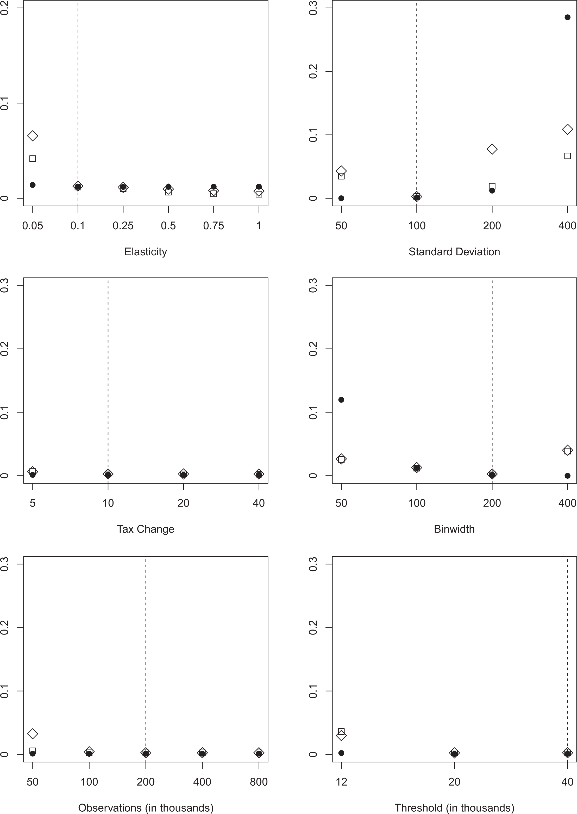
False negatives. Note: The figure depicts the average percentage of false negatives classified using three different approaches for variations in key parameters. We draw 1,000 replications for each specification. BP allowing for two structural breaks is depicted as circles (
The results show that across all specifications, BP (
Perhaps the most striking observation from Figure 2 is the considerable increase in false negatives for Cook’s D and BDS when considering a threshold in the ascending part of the income distribution. This finding mostly hinges on the small number of observations that are to the left of the threshold, when utilizing a binwidth of 100. Following Chetty et al. (2011), we use a maximum of fifty bins on either side of the threshold, and given the nature of our income distribution, we observe relatively few individuals with incomes lower than 12,000. The lower boundary of incomes has a mean of 2,000 and the number of observations is near zero. In this sense, our findings suggest that Cook’s D and BDS perform badly if sample sizes are small. A similar picture emerges when we consider the baseline threshold for top incomes and different sample sizes. As a consequence, we conclude that both Cook’s D and BDS need a sufficiently large number of observations, as well as a significant tax change and elasticity to minimize the number of false negatives. As long as the specification is not too extreme, BP always selects the largest bunching window, minimizing the number of false negatives, and should be the method of choice, if false negatives are the main concern.
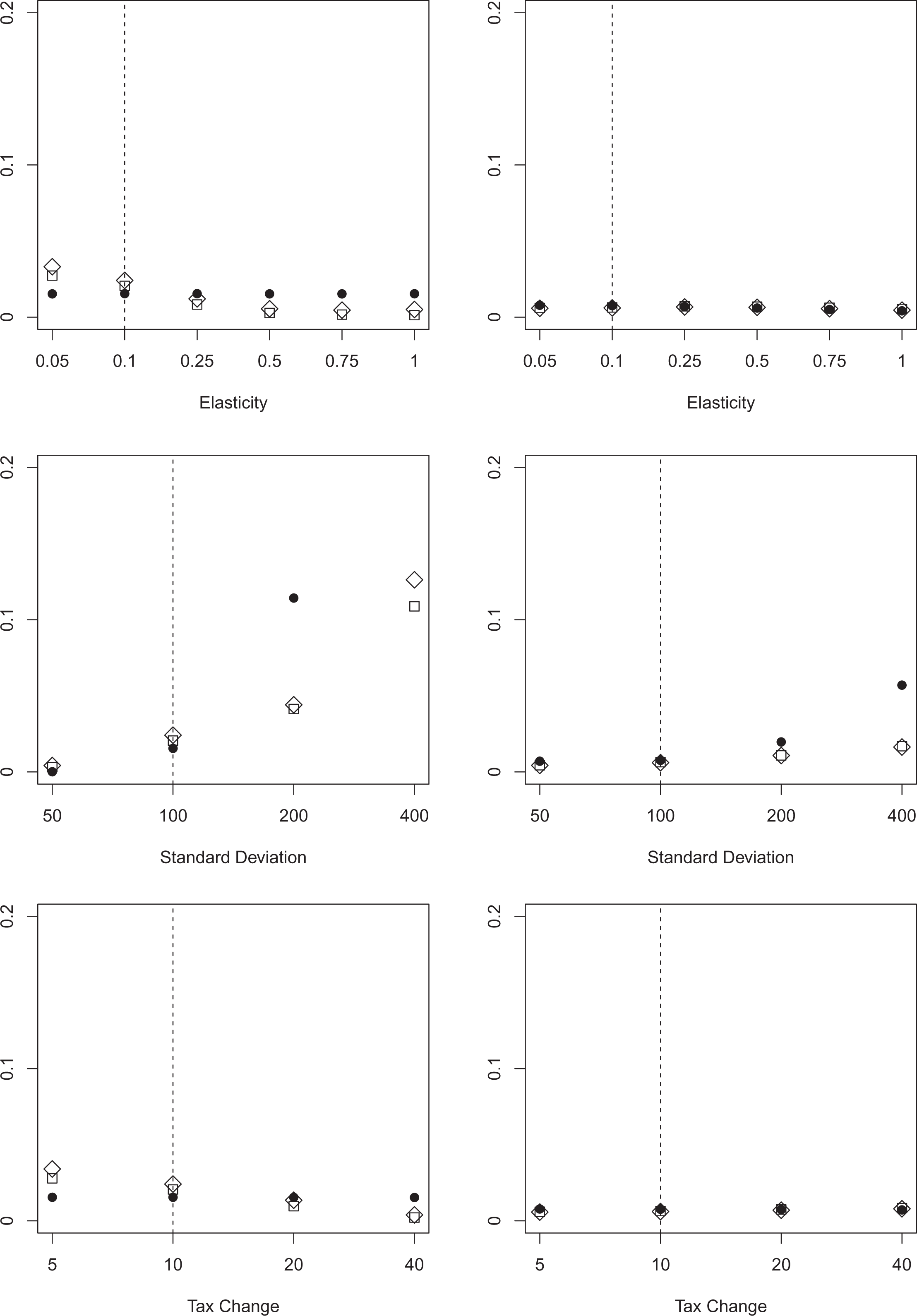
The conservative nature of determining a bunching window using BP, however, comes at the cost of an increased number of false positives. Because of the minimum required distance between two structural breaks, BP delivers a larger bunching window on average and therefore includes more false positives than either Cook’s D or BDS. This finding is robust across all specifications, as shown in figure 3. In line with the results from figure 2, Cook’s D and BDS perform very similarly across all tested specifications.
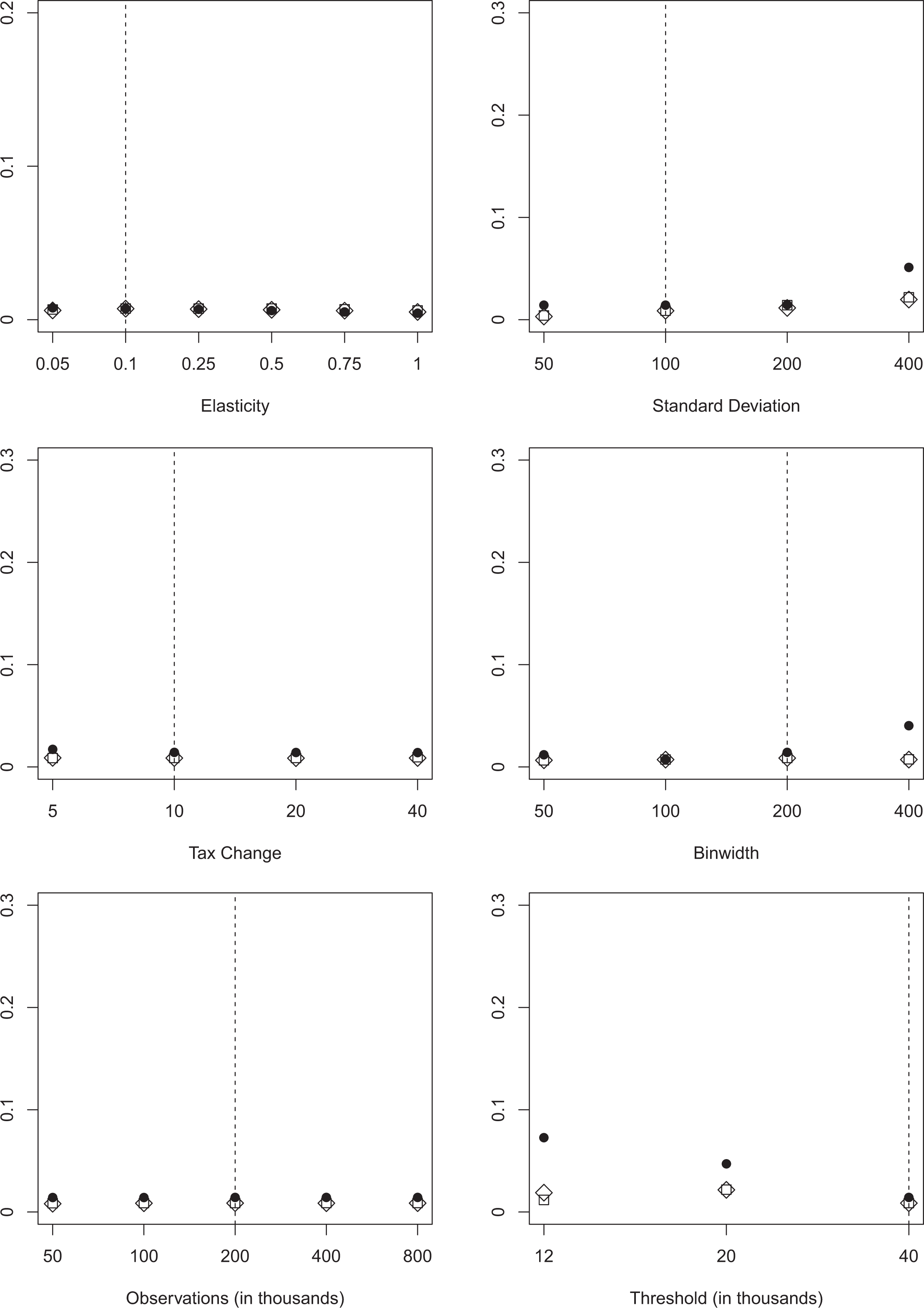
False positives. Note: The figure depicts the average percentage of false positives classified using three different approaches for variations in key parameters. We draw 1,000 replications for each specification. BP allowing for two structural breaks is depicted as circles (
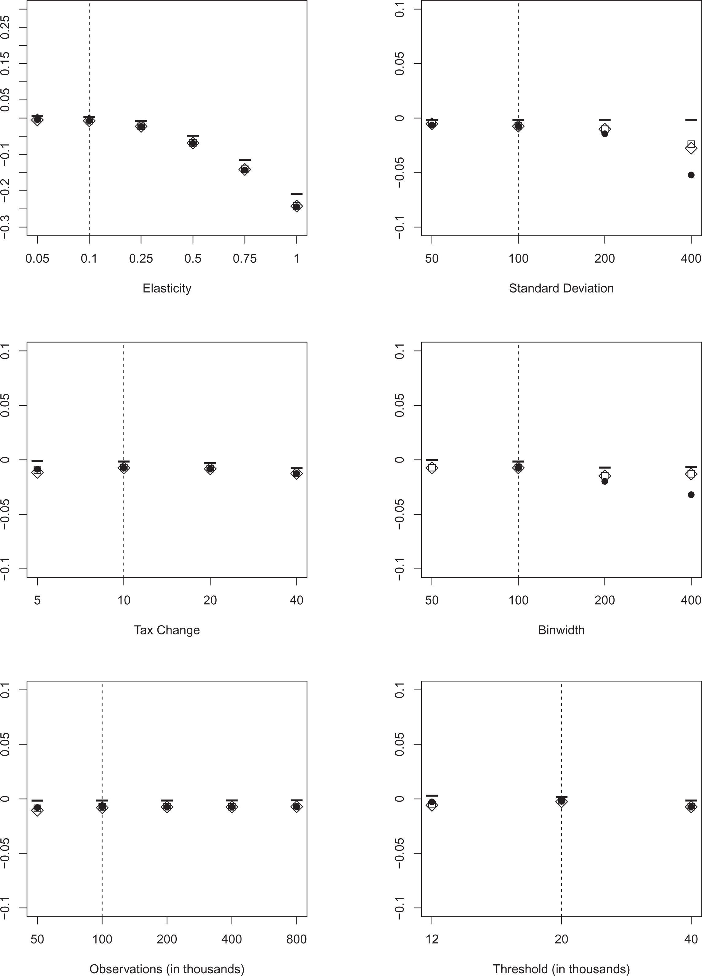
Since no procedure simultaneously minimizes the number of false negatives and false positives, we now consider the average bias of the elasticity estimator in figure 4. These results help us to show how wrongly classifying individuals as bunchers or nonbunchers might affect the results of empirical studies. As we have shown in figures 2 and 3, BP minimizes the number of false negatives but the corresponding number of false positives is larger than for the other two procedures. We always report the average bias of the bunching estimator for a similar configuration without optimization frictions to have a suitable benchmark in situations where the bunching estimator is naturally biased. Additionally, we computed the variance and the mean squared error of the elasticity estimates. Variances are almost identical for all procedures which can be attributed to the large sample sizes generated (motivated by the availability of large administrative datasets for most empirical studies). Hence, we do not report these results. 8
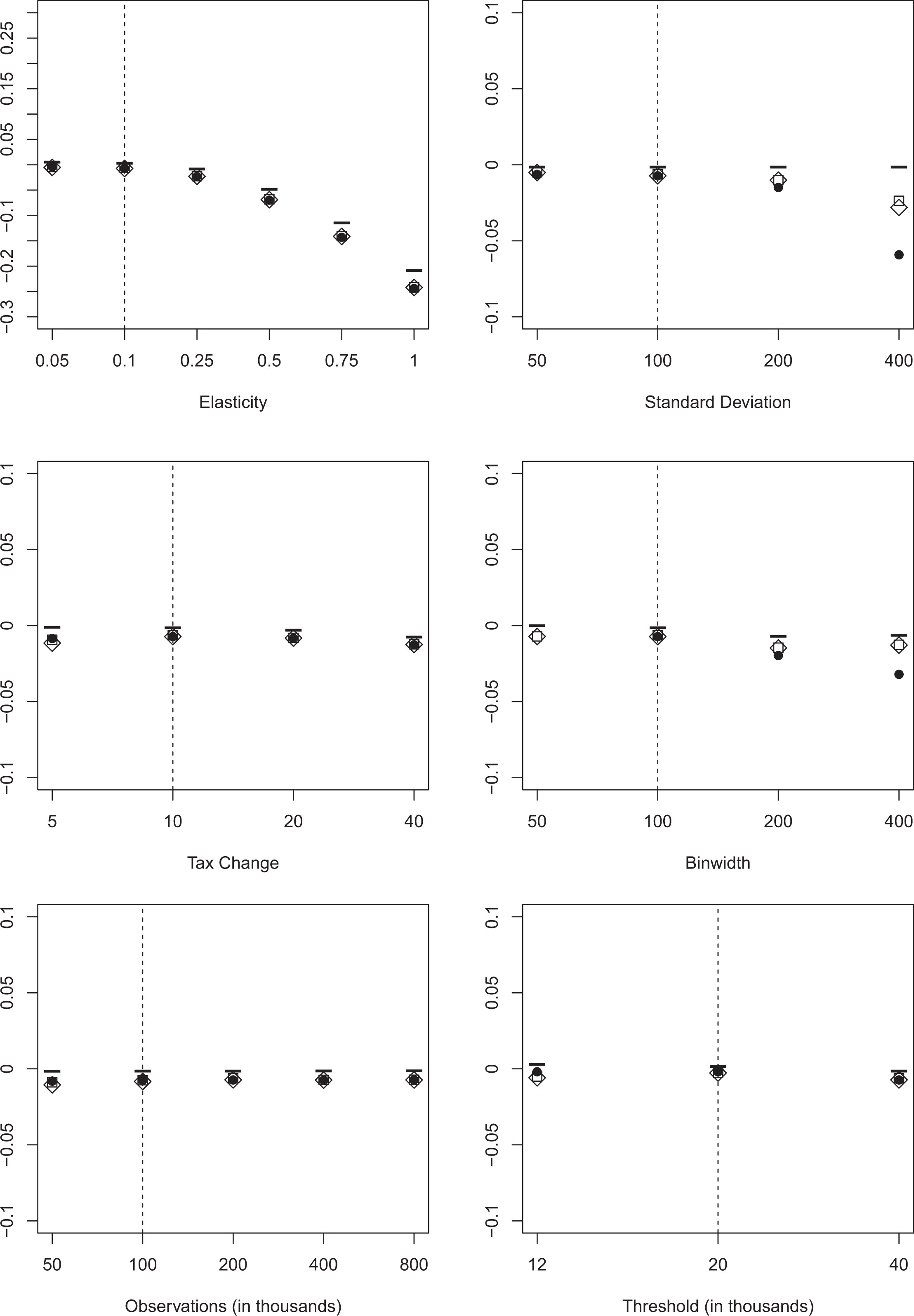
Average bias. Note: The figure depicts the average bias of the elasticity estimator using three different approaches for variations in key parameters. We draw 1,000 replications for each specification. BP allowing for two structural breaks is depicted as circles (
Our results show that the average bias of the benchmark without optimization frictions is surprisingly small if the elasticity is moderate. As expected, we observe the largest bias for the first threshold with the steepest slope and almost no bias at the second threshold located at the mode of our before-tax income distribution. On the basis of the average bias, we have to reject BP as an appropriate method to determine the bunching window because of its sensitivity to more extreme, but realistic specifications. Over most specification, BP has the strongest negative bias and in one specification (binwidth of
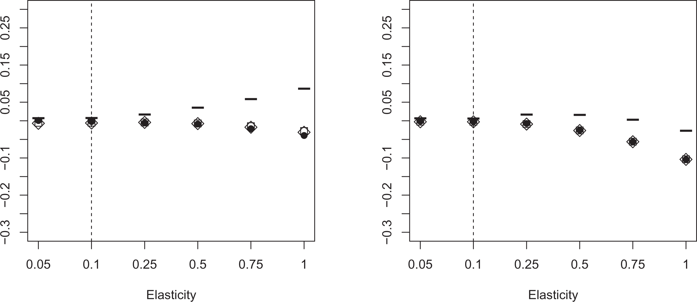
Average bias (alternative thresholds). Note: The figure depicts the average bias of the elasticity estimator using three different data-driven approaches for thresholds located at 12,000 (left) and 20,000 (right). We draw 1,000 replications for each specification. BP allowing for two structural breaks is depicted as circles (
False negatives and false positives for left-skewed distribution. Note: The figure depicts the average percentage of false negatives (false positives) classified using three different approaches for variations in selected key parameters. The left graphs show false negatives, the right graphs show false positives. We draw 1,000 replications for each specification. BP allowing for two structural breaks is depicted as circles (
False negatives and false positives for right-skewed distribution. Note: The figure depicts the average percentage of false negatives (false positives) classified using three different approaches for variations in selected key parameters. The left graphs show false negatives, the right graphs show false positives. We draw 1,000 replications for each specification. BP allowing for two structural breaks is depicted as circles (
We have thus far shown results for estimations, where the bunching window was symmetric around the threshold. But as pointed out by Bosch, Dekker, and Strohmaier (2020), there are good reasons to believe that the bunching window is asymmetric in some cases. We therefore vary the structure of the optimization frictions in such a way that we have more mass to the left (right) of the threshold. For this purpose, we draw
BP overall shows little sensitivity to either the left- or right-side asymmetric specifications, with similar limitations when regarding extreme specifications as in the normally distributed error term case of our baseline specification. Strikingly, an asymmetric bunching window reduces the sensitivity of BP to extreme standard deviations. This finding might be explained by the location of our baseline threshold at a downward sloping segment of the income distribution. Shifting probability mass to the left/right of the kink point creates a more distinctive break which can be detected more easily by the BP procedure. The consistency of Cook’s D, however, seems to be vulnerable when the bunching window is asymmetric around the threshold. Especially with small elasticities and small tax changes, Cook’s D has problems correctly identifying bunchers. The results of the BDS procedure remain consistent with the findings for the symmetric bunching window. In summary, BP delivers the most consistent results when the anticipated optimization frictions are not severe. If optimization frictions are expected to play a significant role, BDS simultaneously minimizes the number of false negatives and false positives. It should therefore be the procedure of choice in empirical applications.
Finally, we follow Patel, Seegert, and Smith (2017) and evaluate the performance of our data-driven methods at several placebo kinks with different slopes. We generate replications without bunching behavior and compute the ETI for thresholds located at 12,000, 16,000, 20,000, 30,000, 40,000, and 50,000 to capture different slopes in the ascending and descending part of the income distribution. Our results are depicted in figure 8. Although the BP procedure requires a minimum number of observations in the middle segment and therefore miss-classifies some nonbunchers, the average bias for all methods is quite small. It seems to be more important to examine large empirical ETI estimates more closely which are often based on wider bunching windows that tend to create problems for the (local) bunching estimator.
Empirical Application
Elasticity of Taxable Income (ETI) Upper Threshold in the Netherlands (2007).
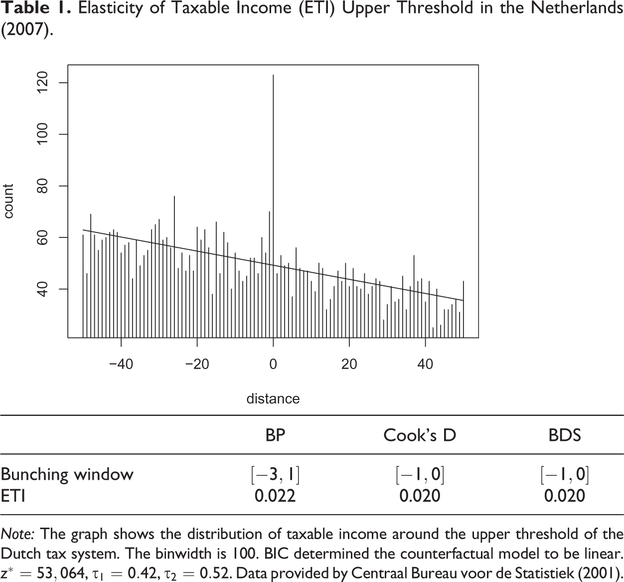
Note: The graph shows the distribution of taxable income around the upper threshold of the Dutch tax system. The binwidth is 100. BIC determined the counterfactual model to be linear.
To further highlight the significant influence that the choice of the bunching window has on estimating the ETI, we analyze a subset of the data utilized in Bosch, Dekker, and Strohmaier (2020). The data come from the public use income panel data (IPO) file from the Dutch central bureau for statistics (Centraal Bureau voor de Statistiek 2001), which is a yearly panel of administrative data that contains exact taxable income. We use the publicly available file for the year 2007 (Centraal Bureau voor de Statistiek 2001) to show the differences in estimated elasticities across the three data-driven procedures. In line with Bosch, Dekker, and Strohmaier (2020), we clean the data from individuals that receive benefits of some sort, are not in the active workforce, or have no income. This is important to abstract from mass points that are generated by other sources than the tax schedule. For example, close to the first threshold, many individuals are located that receive the same amount of (unemployment) benefits. 10 Our sample thus includes 105,112 individuals that are either employed or self-employed.
We start our analysis by looking at the top tax threshold, where the change in the marginal tax rate is biggest and thus, the incentive to bunch is largest. Table 1 first shows the distribution of taxable income around the upper threshold of the Dutch tax system, where the marginal tax rate changes by 10 percentage points. Then, the results from the analysis using the three data-driven procedures discussed in this study are shown. As became evident through the course of this section, Cook’s D and BDS perform similarly and also in this real world application, they both identify the bunching window to be from
Distribution around First and Second Tax Thresholds in the Netherlands.
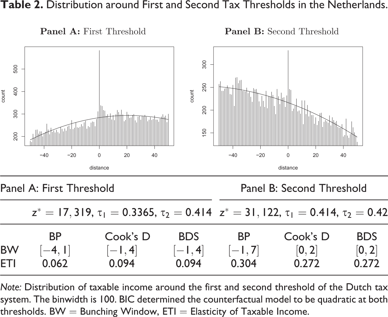
Note: Distribution of taxable income around the first and second threshold of the Dutch tax system. The binwidth is 100. BIC determined the counterfactual model to be quadratic at both thresholds. BW = Bunching Window, ETI = Elasticity of Taxable Income.
Table 2 shows the results for the first (panel A) and second (panel B) threshold of the Dutch tax system in the year 2007. Similar to the findings regarding the top tax threshold, we find the same bunching window using Cook’s D or the BDS procedure, but a different and larger window using the BP method. This translates into a smaller elasticity that is identified at the first threshold using the BP method in comparison to the other two and a larger elasticity at the second threshold.
The empirical findings are in line with our simulation results and highlight the sensitivity of the estimator to the specification of the bunching window. Whilst BP estimates an elasticity that is 10 percent larger at the top tax threshold, it estimates an elasticity that is 51 percent smaller at the first and 11.8 percent larger at the second threshold, when compared to Cook’s D and the BDS procedure. Furthermore, our simulation approach hinted at sensitivities of Cook’s D regarding asymmetric bunching windows. Although none of the bunching windows identified in our empirical application are perfectly symmetric around the threshold, they are not very far off (at least when identified by Cook’s D and BDS). We conclude that the asymmetry of the bunching window needs to be greater than in the Dutch tax system case for Cook’s D to deliver different results than BDS. Because the bunching mass stays quite precisely around the threshold, BP encounters a difficult situation in this application. As we have argued, BP needs, by construction, a certain number of bins inside one regime. This seems to be the reason that BP always finds a larger bunching window than the other two procedures.
Conclusion
We have compared three different data-driven procedures to determine the bunching window in order to elicit, which method is able to identify bunching best. The bunching window should encompass those individuals, who change their behavior and only those. Thus, we set up a framework similar to a classification table and analyze the number of false negatives and false positives, where the former measures how many bunchers the respective procedure fails to detect and the latter measures those individuals that are falsely flagged as bunching. A successful data-driven procedure should ideally minimize both types of errors.
When the bunching window is normally distributed around the threshold, Cook’s D and BDS performed best with slight advantages of BDS over Cook’s D if standard deviations were large or sample sizes were small. Cook’s D stands representative for the general class of outlier detection methods. Further research is necessary to determine whether other outlier detection techniques can be designed to outperform Cook’s D in terms of computational costs and accuracy. BP performed best when the tax change was small or the optimization frictions were not too large. BDS seemed to be the most robust method and showed a balanced performance over all specifications. In a real-world application, we showed that the size of the bunching window has a significant impact on the bunching estimator and subsequently its translation into the ETI. Overall, we conclude that BDS should be the preferred method to detect the bunching window when nothing is known about the true shape of the bunching window although Cook’s D, especially for its ease of implementation, comes a close second.
There are several avenues for future research. Since the standard bunching estimator is only unbiased under restrictive assumptions, robust bunching estimators might be employed which are not based on polynomial regressions. Available estimators in the literature, for example those discussed in Bertanha, McCallum, and Seegert (2019), abstract from empirically relevant optimization frictions and assume that the bunching window is known. Alternative parametric estimators, proposed by Aronsson, Jenderny, and Lanot (2018), explicitly model optimization frictions but require strong distributional assumptions. Further, Cattaneo, Jansson, and Ma (2020) show that the standard polynomial approach does not produce reliable predictions at boundary points, which can be another source of bias of the bunching estimator and propose to use local polynomial density estimators for predicting the counterfactual distribution. It remains an open question how these estimators can be modified to ensure a data-driven determination of the bunching window.
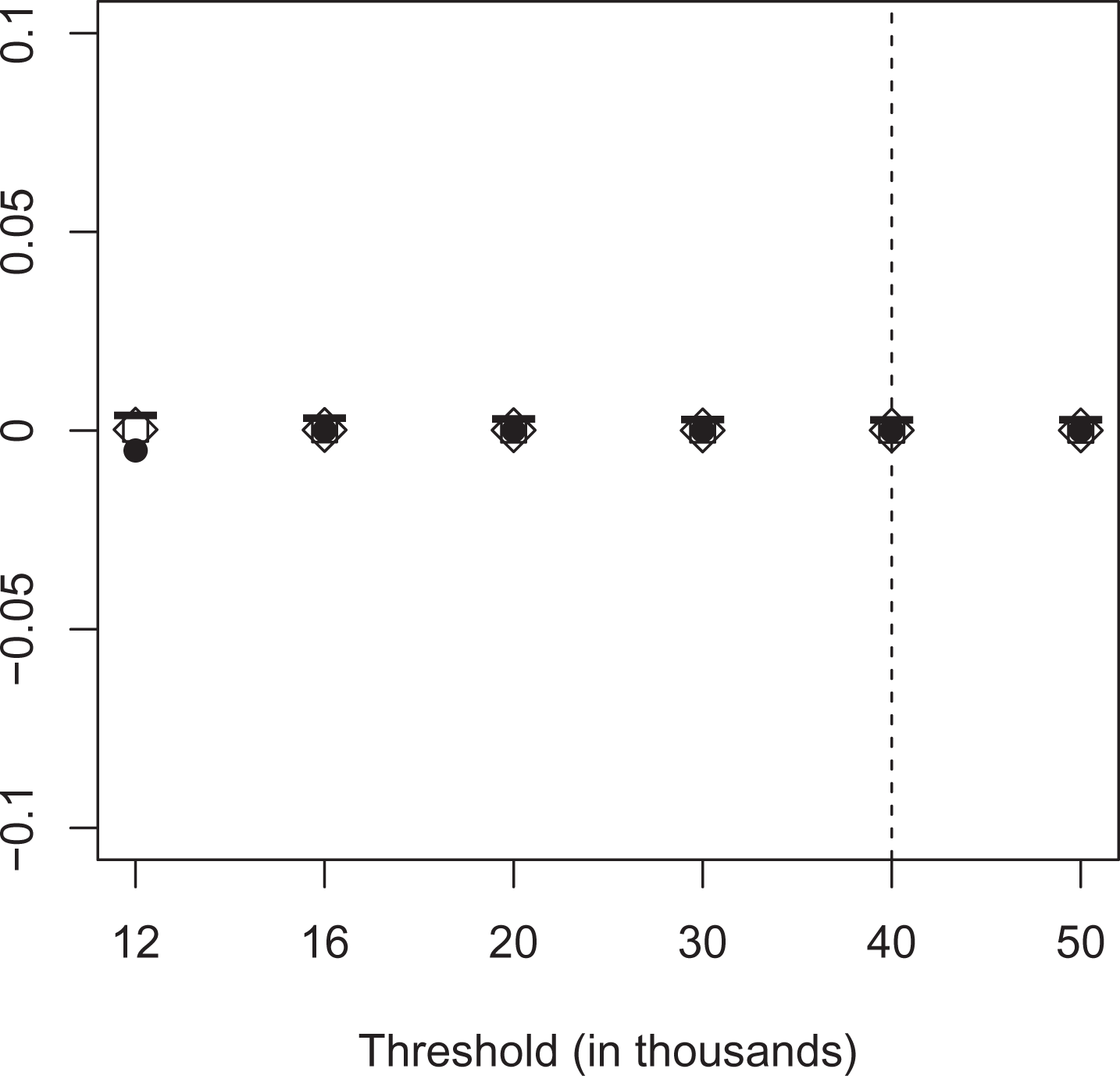
Average bias for different placebo kinks. Note: The figure depicts the average bias of the elasticity estimator using three different approaches for different placebo kinks. We draw 1,000 replications for each specification. BP allowing for two structural breaks is depicted as circles (
Average bias (alternative error specification). Note: The figure depicts the average bias of the elasticity estimator using three different approaches for variations in key parameters. We draw 1,000 replications for each specification. BP allowing for two structural breaks is depicted as circles (
Supplemental Material
Supplemental Material, sj-pdf-1-pfr-10.1177_1091142121993055 - A Comparison of Different Data-driven Procedures to Determine the Bunching Window
Supplemental Material, sj-pdf-1-pfr-10.1177_1091142121993055 for A Comparison of Different Data-driven Procedures to Determine the Bunching Window by Vincent Dekker and Karsten Schweikert in Public Finance Review
Footnotes
Declaration of Conflicting Interests
The author(s) declared no potential conflicts of interest with respect to the research, authorship, and/or publication of this article.
Funding
The author(s) received no financial support for the research, authorship, and/or publication of this article.
Notes
References
Supplementary Material
Please find the following supplemental material available below.
For Open Access articles published under a Creative Commons License, all supplemental material carries the same license as the article it is associated with.
For non-Open Access articles published, all supplemental material carries a non-exclusive license, and permission requests for re-use of supplemental material or any part of supplemental material shall be sent directly to the copyright owner as specified in the copyright notice associated with the article.