
Abstract
The Golden State Killer hunted victims across California from 1974 to 1986. He committed violent crimes in multiple jurisdictions as he escalated from burglary to rape to serial murder. His offending evolution and shifting geography made it difficult for police to connect his crimes, leading to the assumption that different criminals were involved. Over time, therefore, nine separate behavioral profiles were generated for the various investigations. This case study is a comparative analysis of these profiles, their behavioral domains, and specific predictions. Accuracy, consistency, and utility are assessed, and an analytic framework is provided for future assessments and research.
Introduction
From 1974 to 1986, one of America’s most infamous criminals stalked victims across the State of California. He became increasingly violent as he moved from city to city, escalating from burglary to rape to serial murder. First labeled the Visalia Ransacker, he progressed into the Sacramento East Area Rapist and finally the Original Night Stalker. After his crimes were linked by DNA, he became known as EAR/ONS and then the Golden State Killer (McNamara, 2018).
The case was eventually solved through one of the early investigative uses of genealogical DNA. In 2018, Joseph James DeAngelo, Jr., 72 years, was arrested and charged with multiple counts of homicide and kidnapping (the statute of limitations had expired for the rapes and burglaries). He pled guilty and received 11 life sentences with no possibility of parole. DeAngelo is believed to have committed 13 murders, 51 rapes, and 120 burglaries.
To help them identify the killer, police requested a number of psychological/behavioral profiles. The evolution of DeAngelo’s attacks and his geographic shifts made it difficult for detectives to connect his crimes, resulting in the belief that separate offenders were responsible. Consequently, over the course of the various investigations, nine different behavioral profile reports were written. 1
This case study is a comparative analysis of these different profiles. Little research of this nature has been done on behavioral profiling, partly because such reports are typically confidential. It is even rarer to have multiple profiles of the same offender for comparison. A total of 130 predictions, categorized into 13 domains, were extracted from the reports and coded for accuracy and consistency by the author. 2 Operational utility assessments were then made. Finally, recommendations for future research and operational evaluations are presented and discussed within the context of improving expertise.
Golden State Killer
Crimes
The Visalia Ransacker (VR) was active from 1974 to 1975. He was believed responsible for 110 burglaries, one murder, and the shooting of a detective on stakeout. The modus operandi of these burglaries was unusual. As suggested by the name, the offender engaged in extensive ransacking, taking small items such as pictures of teenage girls, a single earring, and loose change. He spent considerable time, often eating and drinking, in the target houses. His burglaries appeared to have a sexual nature, involving peeping, phoning victims, disturbing female underwear, and theft of personal photographs. The VR improvised alarm systems and set up secondary escape plans. There was also a number of bicycle thefts, prowlings, and suspicious telephone calls in the area at the same time. Possibly related, two teenage girls were raped and killed in Tulare County just outside Visalia.
The Ransacker ended his crime spree in Visalia after a close escape from a police stakeout. Six months later, the East Area Rapist (EAR) began his attacks in Sacramento, 220 miles to the northwest, cumulating in a series of 51 rapes and two murders from 1976 to 1978 (Crompton, 2010). The masked offender was armed with a gun and/or a knife. He began targeting lone females and then progressed to male-female couples. The victims were typically attacked in their homes during the early morning while sleeping. EAR sometimes spent hours at the crime site, eating and drinking. The area also suffered burglaries, prowlings, stolen bicycles, and suspicious telephone calls. Visalia and Sacramento investigators debated the possibility that EAR was the Ransacker, but while Visalia police thought they were the same person, Sacramento police apparently did not. Sacramento was displeased when Visalia released the same-offender theory to the media. In 1978, EAR shifted his hunt west to Contra Costa County.
Then, in late 1979, a serial murderer dubbed the Original Night Stalker (ONS) emerged in Goleta, a small unincorporated area in Santa Barbara County, 400 miles south of Sacramento. Couples or lone females were attacked in their beds while sleeping. The victims were bound, males shot or bludgeoned, and females sexually assaulted and beaten. Stolen bicycles were used for transportation. ONS was ultimately responsible for 12 homicides and an attempted double murder in Santa Barbara, Ventura, and Orange Counties in Southern California. His last known crime was a murder in Irvine in May 1986.
Police detectives did not associate these attacks until many years later. Eventually, advancements in DNA analysis established definitive links between the crimes. In 2001, the ONS incidents were connected to the EAR series (now called EAR/ONS). In 2011, additional DNA evidence was recovered using new forensic techniques from a 1981 double murder in Goleta. Law enforcement agencies then finally formed a comprehensive multi-agency task force to investigate all the Golden State Killer (GSK) crimes.
Arrest
In one of many efforts to resolve this very cold case, investigators uploaded the DNA profile from a Ventura County rape kit to the personal genomics website GEDmatch (Holes & Fisher, 2022). The site provides searchers a list of relatives by degree of shared single nucleotide polymorphisms (SNPs), which offer a genetic fingerprint. The percentage of shared SNPs diminishes by familial distance. For example, on average, individuals share only 3.1% of their SNPs with a second cousin.
Out of the 650,000 profiles then on the GEDmatch website, the search identified 10 to 20 distant relatives of the offender (sharing the same great-great-great grandparents, dating back to the 1800s when families often had large numbers of children). From these, a team of five investigators built out more than 25 family trees. Hits came from third and fourth cousins. The tree that eventually linked to the Golden State Killer contained approximately 1,000 people.
Two main suspects were identified from this particular tree—Joseph DeAngelo and his brother. A DNA sample was surreptitiously collected from the door handle of a car Joseph DeAngelo had been driving; a second sample was also recovered from a tissue taken from his curbside trash bin. Both samples were consistent with the Orange and Ventura County suspect profiles.
DeAngelo
Joseph James DeAngelo, Jr., was born on November 8, 1945, in Bath, New York. He had three siblings, one who ended up with a criminal record. His family later moved to California, where DeAngelo went to middle school in Rancho Cordova, and high school in Folsom (both in Sacramento County). His parents divorced when he was in junior high. While in high school, he allegedly abused animals and broke into homes. In 1964, he joined the U.S. Navy and served 4 years during the Vietnam War.
In 1968, DeAngelo enrolled in Sierra College, Rocklin, and graduated with an associate degree with honors in police science in 1970. In 1971, he attended California State University, Sacramento, where he received a bachelor’s degree before going on to do postgraduate work. He did his POST (Commission on Peace Officer Standards and Training) training at the College of the Sequoias, Visalia, and was then an intern with the Roseville Police Department for 32 weeks.
DeAngelo lived in Citrus Heights until he joined the Exeter Police Department where he worked as an officer from 1973 to 1976. He was promoted to sergeant in 1976 and was in charge of an anti-burglary program created because of a rise in crime. He then worked as a police officer in Auburn from 1976 until 1979, until he was dismissed for shoplifting a hammer and dog repellant from a drugstore. He was convicted of theft and sentenced to probation for 6 months.
From 1990 until his retirement in 2017, DeAngelo was a truck mechanic at a supermarket distribution center in Roseville. He was living in Citrus Heights at the time of his arrest in 2018. Credit reports list previous addresses in Whittier and Long Beach.
DeAngelo was married in 1973, and he and his wife had three daughters. They were estranged in 1991. He was also engaged in May 1970 while at Sierra College, but a year later his fiancée called it off because he had become manipulative and abusive. She described him as someone who:
was entitled
was intelligent
was obsessive compulsive
was intimidated by other males
did not drink or smoke
cheated in school
liked to trespass
lacked a conscience
responded with anger to rejection
stalked and threatened her when she ended the engagement.
Behavioral Profiling
Behavioral (also known as psychological) profiling can be defined as the inference of offender characteristics from offense characteristics (Copson, 1995; Douglas et al., 1986). The development of a profile is based on the premise that the interpretation of crime scene evidence indicates the personality features of the responsible individual (Homant & Kennedy, 1998). Certain personality traits exhibit similar behavioral patterns, and knowledge of these patterns may assist in the investigation of the crime and suspect assessment (Ressler et al., 1988). The two major assumptions underlying offender profiling are behavioral consistency—the crimes of the same offender should be similar to one another—and homology—an agreement between an offender’s personality and his/her behavior (Alison et al., 2002; Mokros & Alison, 2002).
The criminal profiling process asks three basic questions:
What happened at the crime scene?
Why did these actions occur?
Who would have done this?
To be successful, not only must a profile be reasonably accurate, but it must also possess operational utility (Rossmo, 2011). Despite the Hollywood image, profiling cannot solve a crime; only a witness, a confession, or physical evidence can do that (Klockars & Mastrofski, 1991). An FBI in-house survey of 88 BSU profiles for crimes that had been later solved found their main contribution was helping to focus the investigation (Institutional Research and Development Unit, 1981). Research on profiling in the Netherlands established that detectives obtained the most value from investigative suggestions and interviewing techniques; they regarded the profiles themselves as sometimes too vague (Jackson et al., 1993). Detectives also benefited from the profilers’ independent perspective and their expertise with bizarre crimes.
Profile predictions are probabilistic, so the process can only play a supporting role in police investigations. That role can be considered within two distinct contexts (Rossmo, 2021). The first is strategic. There is often a need at the beginning of a stranger violent crime investigation to prioritize large numbers of tips, registered sex offenders, parolees, suspects, and so on. Profile details that are commonly included in computerized databases (e.g., age, location) can be used for this function. The second is tactical. Once a prime suspect has been identified, a profile can help guide police actions to resolve the case by providing behavioral insights. These help detectives develop interview strategies and may suggest other possible crimes in a series. The strategic context is more actuarial, the tactical more clinical. While there may be other applications (see Beauregard et al., 2007), these are the two primary uses of criminal profiles.
Case Profiles
The various profiles 3 in this case were prepared over the years by different individuals/agencies for requesting law enforcement jurisdictions (see Table 1). The FBI began providing a level of support for violent crime investigations in 1978; however, the National Center for the Analysis of Violent Crime (NCAVC), within which the original Behavioral Science Unit (BSU), was housed did not become operational until 1986 (Depue, 1986; Douglas & Burgess, 1986). Consequently, law enforcement agencies often turned to psychiatrists and psychologists to help them understand the type of criminal they were trying to catch. The comparisons in this analysis are more apples-to-oranges because the profiles are based on different subsets of the GSK crimes and the reports do not follow a standard format. They are consistent in one manner, however—they all focus on the same offender. Only the last profile, written in 2013, was based on all the known crimes.
Golden State Killer Profiles.
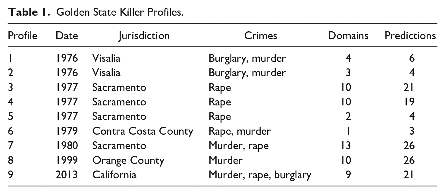
Data
From 1976 to 2013, nine different profiles were generated for the various police investigations. Two of the reports were arguably more crime analysis than behavioral profiles, though the distinction is not always clear. 4 The profiles were primarily written by psychologists, clinical staff, and consultants, but two were created by law enforcement behavioral science specialists.
The various profile predictions were grouped into 13 common domains identified from the nine reports:
age
geography (current or past residence/work site)
crime behavior (likely criminal record, risk of offending progression)
family (familial relationships)
personal circumstances (lifestyle)
work
intelligence
general behaviors (noncriminal activities)
psychological disorders
sexual (sex problems/disorders)
anger (excessive rage)
social (relationships with others)
personality.
Table 1 lists the dates, jurisdictions, and crimes analyzed in each of the nine profiles, along with the number of domains and predictions in the respective report. A prediction was a specific claim about the offender or his crimes (e.g., was in the military; will reoffend). There was a total of 130 predictions. 5
Analysis
There was some variation in the number of predictions per profile (mean = 14; median = 20; range 3–26). Of the 130 predictions, 47% were judged accurate, 33% inaccurate, and 20% remain unknown (the accuracy for all known predictions was 59%). The most accurate predictions were in the social, geography, psychological disorder, personality, intelligence, and crime behavior domains. The least accurate related to age, 6 personal circumstances, and work. Individual profile accuracy averaged 54%, and ranged from a high of 75% to a low of 29% (note this analysis is not intended to be a competition). Inaccurate predictions averaged 29%. The sexual domain contained the highest proportion of unknown accuracy predictions (73%). There was no relationship between when the profile was prepared and its accuracy.
Profile consistency (i.e., similar predictions made in different profiles) averaged 42%. Consistency might only reflect a feature’s high base rate, while the absence of consistency may simply result from a different focus by the profiler. More critical are inconsistencies (e.g., extreme guilt vs. lacking remorse), as these risk pointing an investigation in different directions. At least one of the inconsistent predictions must be wrong. Conflicting predictions occurred 10% of the time.
Consistent predictions are not necessarily accurate predictions. The highest consistencies occurred in the social, sexual, psychological disorder, family, and personality domains. The lowest consistency occurred in the psychological disorder domain. Table 2 shows profile accuracy and consistency by domain.
Profile Results.
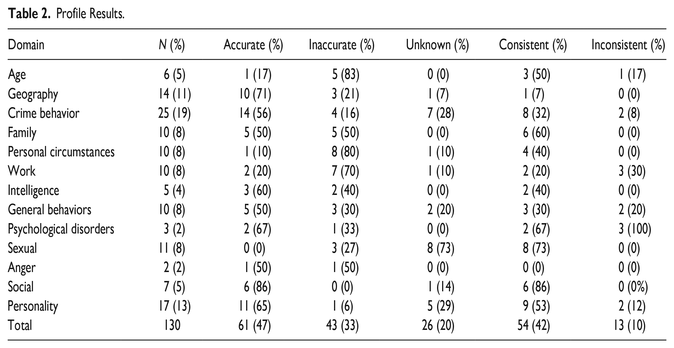
Table 3 lists the 13 profile domains assessed by their potential strategic and tactical utility. The following ordinal scores were used:
Profile Domain Utility.
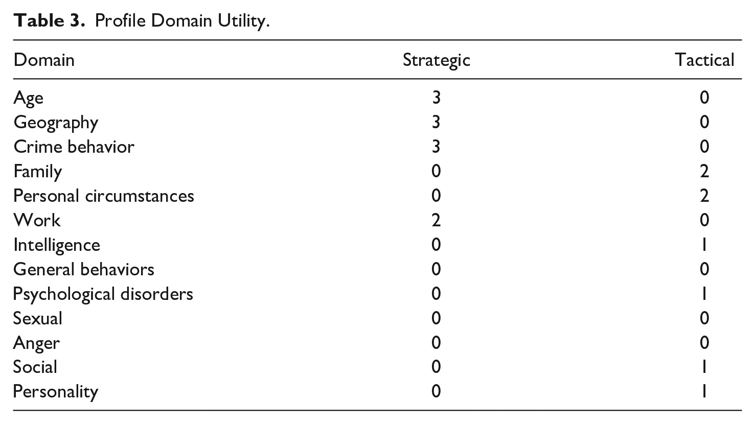
0 = not useful (there was no discernible investigative value in the prediction).
1 = possibly useful (the prediction may possess some utility but only under limited case conditions).
2 = somewhat useful (there appears to be value in the prediction, but it cannot be used for search/prioritization purposes).
3 = definitely useful (the prediction could be used in the strategic context to guide the search and prioritization of database records).
This assessment was derived from specific profile predictions. Other factors, not mentioned in the GSK case, could potentially increase the utility of a domain.
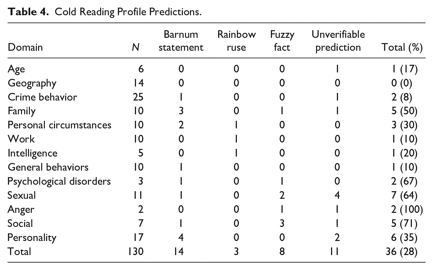
Profiles have long been criticized for being vague or too general. The specific language and nature of some predictions may be unverifiable or even contradictory, capable of supporting multiple interpretations (Alison et al., 2003). In a critical comparison of psychological profiling to cold reading, Gladwell (2007) identified the following problematic prediction types: (1) a Barnum statement is a general assertion with no differentiating value; (2) a rainbow ruse includes both a trait and its opposite; (3) a fuzzy fact is imprecise, ambiguous, noncommittal; and (4) an unverifiable prediction is a claim that cannot be established as true or false (see Rowland, 2005). Note that these categories may overlap to some degree.
Table 4 lists the numbers of instances of these four issues found in each domain for the nine profiles. Vagueness undermines a prediction’s utility (even if it is judged to be accurate). As noted, there is a degree of subjectivity. It is also difficult to claim with certainty that a prediction would never be useful in an investigation, particularly after a particular suspect has been identified. Still, this breakdown helps illuminate which particular domains may be more or less troublesome. In the GSK case, the anger, social, psychological disorders, and sexual domains involved the highest proportion of “cold reading” predictions.
Cold Reading Profile Predictions.
Discussion
Assessments of profiling typically consider the accuracy, reliability, and utility of predictions. For a profile to be useful, it must assist in the investigative decision-making process. Equivocal, unworkable, or improbable suggestions will not produce helpful leads. The contribution of a behavioral profile to a criminal investigation ultimately depends on its use in an operational context.
A review in the United Kingdom of solved cases involving profiling advice determined that 72% of predicted offender characteristics (N = 114) were correct, 19% were incorrect, and 9% lacked sufficient information for classification (Goldblatt, in Copson, 1995). In the GSK case, individual profile accuracy averaged 54%, ranging from a high of 75% to a low of 29%. However, there is a problem when comparing individual results because the number of predictions varied between profiles. A profile that focuses on “safe” predictions (i.e., the more probable or obvious) will almost certainly be more accurate. However, this may come at the loss of operational utility. There was a moderate negative correlation (r = −.70, p < .05) between the number of predictions in a profile and its overall accuracy rate.
Even a high accuracy rate in a profile has limited value if it is not known which specific predictions are correct. For example, a 70% accuracy rate in a given case means 30% of the predictions were wrong—but which ones? There is also variability between profiles (and undoubtedly between profilers).
Arguably more important than comparing individual profile accuracy is an analysis of domain accuracy. The most accurate predictions were in the social, geography, psychological disorder, personality, intelligence, and crime behavior domains. The social and personality domains also exhibited relatively high consistency. The least accurate predictions related to age, personal circumstances, and work.
These results provide a measure of consistency and homology (accuracy) at the domain level. They also identify certain types of prediction likely to be problematic. While the majority of predictions were not of the “cold reading” type, these were still more common than desirable. It is important for profile reports to be as clear, specific, and precise as possible. It would also be helpful if profilers assigned at least rough confidence levels to their predictions.
This study argues for profile-operational integration. The potential application of a prediction—whether it could be used for strategic or tactical purposes—should be articulated and explained. Characteristics most helpful for the former task are those that can be applied in database searches/prioritization, such as personal descriptors, (age, sex, race/ethnicity), addresses, criminal records, occupational history, and the like. It should be remembered that a profile is not a psychiatric diagnosis; the objective is arrest, not treatment.
While information management is a less sensational use of psychological profiling than what is typically shown in film or television portrayals, this functionality is important. The Golden State Killer is an excellent illustration of the challenge and need for empirically-based suspect prioritization methods. The task force’s initial Sacramento data dump, focusing on white males born between 1940 and 1960, resulted in 485,816 names (1,105,856 addresses), later refined to 179,894 unique persons/addresses. All addresses were geocoded and then prioritized using Bayesian probability. The top 100,000 of this group (56%) then had to be compared to various suspect databases (~10,000 entries).
This integrated evidence-analysis approach is exemplified by Operation Lynx, a large-scale serial rape investigation in England (Rossmo, 2013). Police had recovered DNA from the victims, but the offender was not in the UK national DNA database. However, investigators found a partial fingerprint at one of the scenes. As there was an insufficient number of points for a computerized search using AFIS (automated fingerprint identification system), police had to conduct a hand search. This was a daunting task as the inquiry had identified over 12,000 suspects. To handle this information overload challenge, the task force developed a suspect prioritization strategy based on victim descriptions, behavioral profiles, a geographic profile, and other factors.
White males from Leeds, 35 to 52 years of age (from victim descriptions), residing in either the Millgarth or Killingbeck neighborhoods (from the geographic profile), with a criminal record for minor offenses (from the behavioral profiles), were prioritized. Following this strategy, police eventually identified a corresponding fingerprint from Clive Barwell. His DNA matched that recovered from the rapes, and he confessed. This case is an excellent illustration of how physical evidence, behavioral assessments, spatial analysis, and victim/witness observations can be effectively integrated to identify a stranger offender and solve a major crime series.
Limitations
This analysis is a type of natural experiment, not a controlled study (such an option does not exist during a criminal investigation). The profiles were written at different times by separate individuals based on varying subsets of the GSK’s crimes. The numbers are relatively low. Statistical significance is not applicable because we are not dealing with a sample. Any attempt to analyze, compare, and learn from this study has to work around its operational realities.
Recommendations and Conclusion
Behavioral profiles are probabilistic descriptions of the offender responsible for a crime or crime series. They must be constructed to align with police strategies if they are to have any operational value. While a profile cannot solve a crime, it can be useful when combined with other investigative approaches. Such utility is enhanced when a profile is integrated with different evidence types—physical, witness, and/or spatial-temporal. Database searches and suspect prioritization, such as familial and genealogical DNA queries, benefit from behavioral and geographic analyses (Gregory & Rainbow, 2011). Bayes’ theorem provides the mechanism for integrating probabilities from different evidence types (Blair & Rossmo, 2010; Taroni et al., 2006).
This study found profile predictions from certain domains more likely to be accurate, consistent, and/or operationally useful. While the findings provide some guidance for improving profile performance, further research and replication is required. In particular, we need a better understanding of the causes of inaccurate predictions. Unfortunately, the logic, rationale, conventions, and assumptions underlying most of the profile predictions in the GSK case were not articulated in the available reports. Certain domains are more variable than others, and establishing conditions under which the consistency and homology assumptions are justified is essential. Efforts to improve utility, on the other hand, are more straightforward and can be accomplished through greater understanding and more communication between investigators and profilers.
The approach outlined here provides a framework for configuring future research studies. Moreover, law enforcement agencies that provide behavioral profiling services should, following an offender’s identification, routinely assess what the profile got right, what it got wrong, what was useful, and what was missed. This framework could also be employed for that purpose. One of the important requirements for developing expertise is experience. But experience alone is insufficient; feedback is also necessary (Kahneman, 2011; Kahneman & Klein, 2009). We can’t improve if we don’t learn from experiences—both successes and failures.
Footnotes
Acknowledgements
The author wishes to acknowledge the helpful comments, insights, and presentations of Lorie Velarde, Dr. David Stubbins, Paul Holes, and the manuscript reviewers. Lorie Velarde is a crime analyst and geographic information system (GIS) specialist with the Irvine Police Department in California. She was a member of the Golden State Killer Task Force. Dr. David Stubbins is a forensic psychologist and a former Central Intelligence Agency officer. He has consulted with numerous California law enforcement agencies in criminal investigations. Paul Holes is a retired forensic scientist and cold-case investigator for the Contra Costa County Sheriff’s Office in California. He was a member of the Golden State Killer Task Force and played a key role in identifying DeAngelo through the innovative use of DNA genealogy.
Declaration of Conflicting Interests
The author declared no potential conflicts of interest with respect to the research, authorship, and/or publication of this article.
Funding
The author received no financial support for the research, authorship, and/or publication of this article.