Sage Journals: Discover world-class research

Abstract

This study aims to contribute to understanding urban spatial and temporal patterns of social disorganization and homicide rates in São Paulo, Brazil (2000–2015). Using exploratory spatial data analysis and spatial panel regression techniques, we describe spatial-temporal patterns of homicide rates and assess to what extent social disorganization can explain between-district variation in homicide trajectories. The results showed some variation in the pattern of homicide decline across districts, and less disorganized communities experienced earlier, more linear declines. However, we found no evidence to suggest that changes in social disorganization are associated with differences in the decline in homicide rates.

Keywords

social disorganization structural correlates spatial analysis homicide decline trends mapping

In the past three decades, homicide rates have declined dramatically in cities across much of the western world (Baumer & Wolff, 2014; Farrell et al., 2010; Goertzel et al., 2013), but continue to rise in many parts of Latin America (Tuttle et al., 2018). Closer examination of spatial and temporal variation in homicide rates reveals significant heterogeneity between and within Latin American countries (Muggah et al., 2016). In Brazil, where national homicide rates have risen steadily since 1980, the municipality of São Paulo has experienced a dramatic reversal and decline in the early 2000s (Goertzel & Kahn, 2009). Between 2000 and 2007, the number of homicides fell by 78% (Freire, 2018). Known as the “great São Paulo homicide drop,” the case has been the subject of scientific scrutiny and debate over the possible causes contributing to the decline (De Mello & Schneider, 2010; Freire, 2018; Goertzel & Kahn, 2009; Goertzel et al., 2013; Peres et al., 2012).

However, homicide rates are highly unequal across urban space (Baumer et al., 2018; Ceccato et al., 2007; Cohen & Tita, 1999; Light & Harris, 2012; Ye & Wu, 2011). Spatial analyses suggest that homicide is concentrated in poorer, socially disorganized neighborhoods within cities (Ceccato & Oberwittler, 2008; de Melo et al., 2017; Escobar, 2012; Morenoff et al., 2001; Valasik et al., 2017; Zeoli et al., 2014). Social disorganization refers to the process by which ecological conditions such as poverty, high residential mobility, and poor living conditions weaken community capacity to build ties and collectively regulate social norms (Kawachi et al., 1999; Sampson & Groves, 1989; Sampson et al., 1997).

Despite this growing attention to variations in homicide declines in Latin American cities, few studies have assessed the extent of variation at smaller spatial units of analysis (Pereira et al., 2017). By assessing spatial-temporal patterns of homicide rates within a single city, we will be better able to understand the uniformity of the decline between districts, and disentangle the extent to which trends are driven by socio-economic structural transformations compared to other shared underlying factors (Tuttle et al., 2018). This study therefore aims to contribute to knowledge on urban spatial and temporal patterns of social disorganization and homicide using the case study of São Paulo. Specifically, we explore variation in temporal patterns of homicide rates between districts in São Paulo, and assess to what extent trajectories can be explained by social disorganization.

Social Disorganization and Homicide Rates

Researchers aiming to understand why crime is concentrated in poor urban communities typically draw on social disorganization theory (Shaw & McKay, 1942; Stults, 2010). Recent developments in social disorganization theory focus on how the structural characteristics of disadvantaged neighborhoods, such as residential instability and poverty, disrupt the social ties, and networks necessary to foster informal social control (Sampson & Groves, 1989; Sampson et al., 1997; Hipp & Wickes, 2017).

While there is ample cross-sectional evidence that residents in socially disorganized communities are at higher risk for violent crime and homicide (e.g., Breetzke, 2010; de Melo et al., 2017; Hipp & Wickes, 2017; Pereira et al., 2017; Vilalta & Muggah, 2014), evidence is less clear whether changes in social disorganization lead to changes in homicide rates (Steenbeek & Hipp, 2011; Stults, 2010). Longitudinal studies of social disorganization and violence are scarce (Wickes & Hipp, 2018). One issue is that structural characteristics of neighborhoods are “remarkably stable” in their relative ranking over time (Sampson & Morenoff, 2006, p. 199), particularly compared to homicide rates, which tends to show greater variation over time (Martinez et al., 2010). This means that neighborhood structural characteristics may not vary enough over time to fully explain changes in homicide rates. Nevertheless, studies have demonstrated that short-term changes in social disorganization, particularly indicators of disadvantage (e.g., median income, household structure, and living conditions), are associated with changes in violent crime (Cerdá et al., 2012; Hipp & Wickes, 2017; Kikuchi & Desmond, 2010; Martinez et al., 2010; Stults, 2010).

Another issue is that longitudinal panel studies rarely account for the spatial autocorrelation, or clustering, of homicide (Ye & Wu, 2011). Studies that have investigated spatial-temporal patterns of violence have found that the degree of spatial clustering between geographical units can vary over time (Kikuchi & Desmond, 2010; Osorio, 2015). Likewise, “hot” and “cold” spots of homicide within cities are not always located in the same areas over time (Valasik et al., 2017; Ye & Wu, 2011). This spatial clustering has both substantive and empirical implications for how we understand variations in homicide rates across time and geographical space (Baller et al., 2001). Substantively, spatial analyses have illuminated how homicide and other types of violence can spread (or recede) across neighborhoods through diffusion processes (Cohen & Tita, 1999; Loeffler & Flaxman, 2018; Messner et al., 1999; Tita & Radil, 2010). Empirically, ignoring spatial autocorrelation can lead to biased estimates of effect (Anselin, 2013).

Social disorganization can play an important role in the diffusion of homicide across geographical space. Socially disorganized neighborhoods lack the capacity for community control, increasing opportunities for illegal markets, the spread of deviant norms, and conflict (Fagan & Davies, 2004; Griffiths, 2013). Social disorganization can also create conditions favorable to the emergence and spread of criminal and organized crime groups, as residents are often neglected by state security services and lack the collective capacity to confront these groups (Cardia et al., 2003; Oliveira et al., 2015; Rengert et al., 2005). For example, Zeoli et al. (2014) found that the diffusion of homicide hot spots in Newark, New Jersey was consistent with the spread of drug markets and gangs in disadvantaged neighborhoods. Disadvantaged neighborhoods may therefore be more susceptible to contagion processes, particularly when they are spatially and socially proximate to one another (Fagan & Davies, 2004; Mears & Bhati, 2006).

It is important to note that while a number of studies have shown associations between characteristics of social disorganization and violence in Latin America (Escobar, 2012; Pereira et al., 2017; Peres & Nivette, 2017; Vilalta & Muggah, 2014), there is still some debate regarding the generalizability of underlying mechanisms. In particular, studies have found that social disadvantage is not necessarily associated with weaker social ties or a loss of social control (de Melo et al., 2017). In Belo Horizonte, Brazil, disadvantaged neighborhoods were found to have higher levels of social cohesion, although this did not translate into lower crime in the community (Villarreal & Silva, 2006).

Likewise, organized crime groups and gangs concentrated in socially disadvantaged neighborhoods often act as agents of social control (Escobar, 2012). In São Paulo, ethnographic studies have pointed to the emergence of the criminal group the Primeiro Comando da Capital (PCC) in marginalized favelas as an important factor in contributing to homicide declines (Biderman et al., 2019; Willis, 2015). The PCC emerged as a response to overcrowding, feelings of arbitrariness, and precarious living conditions among prisoners in São Paulo prisons (Adorno & Salla, 2007; Dias, 2009, 2013; Feltran, 2010). Studies are consistent in demonstrating that the PCC can play a role in mediating local conflicts, instituting a parallel and illegal justice mechanism that operates in the form of “debates” that simulate jury courts, as well as investigate, judge, and sentence local crimes and disputes of distinct gravity. One of the results of this mechanism would be a certain “pacification” of the territories with the consequent fall in homicide rates in these areas.

The Current Study

Taking these issues into account, we build on existing research on social disorganization and homicide decline in two ways. First, we utilize exploratory spatial data analysis to describe spatial-temporal variation in homicide rates during a period of significant decline (2000–2015). Second, we use spatial panel regression techniques to assess to what extent the level and change in social disorganization in São Paulo districts is associated with variation in homicide trajectories, while accounting for spatial autocorrelation.

Methods

Data and Measures

The Municipality of São Paulo is divided in 96 administrative districts. Data on death due to Aggression (X85-Y09), legal intervention (LI) (Y35-Y36) and external cause due to undetermined intent (ECUI) (Y10-Y34) were obtained from the Mortality Information System (Programa de Aprimoramento das Informações sobre Mortalidade) from the Municipal Health Department of the city of São Paulo for all 96 administrative districts between 2000 and 2015, resulting in a total of 1,536 district-years. By law, external cause of death is classified according to the 10th Revision of the International Classification of Diseases (ICD-10) in death certificates by a coroner after a necroscopic examination. In Brazil, it is well recognized that homicide counts are underestimated when based only on death classified as aggression (X85-Y09), because of the failure to establish intentionality. This results in a high proportion of deaths classified as ECUI and can bias time-series analysis (Cerqueira, 2012; Soares-Filho et al., 2016). It is also widely recognized that police killings account for a high proportion of homicides in São Paulo, but only recently these deaths are being coded as death due to legal intervention (LI) (Y35-Y36).

In order to account for these potential biases, all cases coded following the ICD-10 classification as X85-Y09, Y1-Y34, and Y35-Y36 were included in our study. Since our main interest is the study of homicide rate trajectories, which are highly influenced by changes in the quality of death classification over time, we chose to adjust for this issue by reclassification based on the best quality information on external cause deaths due to undetermined intent (UI), following the same approach used in previous studies on Brazilian homicide (Peres & Nivette, 2017; Soares-Filho et al., 2016). Following the Bogotá Protocol (Cámara de Comercio de Bogotá, 2015) we also considered as homicide all deaths due to LI. The Bogotá Protocol proposes an integrative concept of homicide, not limited to its legal definition, as “the death of one person caused by the willful assault of another,” including those committed by public agents in the exercise of their professional duty, even when legal. By adopting a non-legal concept of homicide, the Bogotá Protocol aims to (i) maximize international comparison; (ii) incorporate as a focus of preventive strategies all intentional violent deaths, regardless of their legality, and (iii) avoid the delay in data analysis, disconnecting them from the judicial decision (Cámara de Comercio de Bogotá, 2015; Fórum Brasileiro de Segurança Pública, 2016). In this way we were able to minimize bias in the time-series resulting from the under-estimation in the number of homicides due to incorrect classification.

We used the year 2000 World Health Organization’s standard population for the direct standardization of homicide rates by age group (0–4; 5–9; 10–14; 15–19; 20–29; 30–39; 40–49; 50–59; 60+), resulting in age-standardized homicide rates for each district and year. Data on population size by age groups were drawn from the Health Department Information System of the city of São Paulo. For analyses, the natural log of the homicide rate was taken in order to adjust for skewness.

The explanatory variables were selected to reflect different dimensions of socioeconomic disadvantage as a source of social disorganization. Socioeconomic disadvantage is said to negatively impact the structure and strength of social ties, and consequently the community’s capacity to control crime (Sampson & Groves, 1989; Sampson et al., 1997). We include five indicators of socioeconomic disadvantage: the proportion of households whose heads earn between zero and five times the minimum wage, the proportion of favelas and crowded domiciles, and the proportion of households with access to sewage and garbage collection. The latter three variables reflect the quality of a community’s living conditions, in which crowding within households and a lack of access to basic amenities are typical social structural characteristics of slums (Perlman, 2006; Unger & Riley, 2007). The quality of living conditions has been used as an indicator of social disadvantage and disorganization in previous research in Latin America (de Melo et al., 2017; Vilalta & Muggah, 2014). All five variables are measured at two time points: 2000 and 2010. The indicators of socioeconomic disadvantage were drawn from census data available from the Brazilian Institute of Geography and Statistics (Instituto Brasileiro de Geografia e Estatística, n.d.).

In order to avoid multicollinearity and maintain a parsimonious model, we conducted principle-component factor analysis to generate one aggregate indicator of social disorganization at each time point (McCall et al., 2010). Each variable was z-standardized prior to analysis. The one-factor solution explained 61% of the variance in 2000, and 57% in 2010. Both scales can be considered reliable with Cronbach’s alphas of .83 in 2000 and .80 in 2010. The social disorganization factor scores have a mean of 0 and standard deviation of 1. Next, a change score was computed by subtracting social disorganization scores for the year 2000 from 2010 scores. Positive values therefore reflect increases in social disorganization over the 10-year period, whereas negative values reflect decreases in social disorganization.Table 1 provides a breakdown of average values for each component within the social disorganization scale at less than 1 standard deviation below the mean, between −1 and +1 standard deviation, and +1 standard deviation above the mean.

Table 1.

Breakdown of Characteristics for Each Component of the Social Disorganization Score by Level of Social Disorganization.

	Social disorganization score: less than/equal to 1 SD		Social disorganization score: between ±1 SD		Social disorganization score: greater than/equal to 1 SD
	Mean	SD	Mean	SD	Mean	SD
Year 2000
Proportion of households with garbage collection	99.99	0.02	99.46	0.78	95.48	7.65
Proportion of households with sewage connection	99.38	0.61	91.93	6.75	58.84	26.43
People living in the same household (crowding)	2.69	0.19	3.47	0.25	3.85	0.11
Proportion living in favelas (slums)	0.04	0.07	0.83	1.09	3.14	2.83
Proportion of household heads in lowest income level	13.01	5.78	33.78	12.26	57.69	7.41
N	12		71		13
Year 2010
Proportion of households with garbage collection	99.94	0.09	99.85	0.26	98.50	2.94
Proportion of households with sewage connection	99.50	1.15	94.50	4.50	71.66	28.08
People living in the same household (crowding)	2.47	0.21	3.16	0.23	3.43	0.11
Proportion living in favelas (slums)	0.08	0.09	0.84	0.85	3.43	2.04
Proportion of household heads in lowest income level	25.47	10.38	54.31	16.13	76.65	3.86
N	16		73		11

Note. SD = standard deviation.

We include a measure of property crime rates per 1,000 population in order to control for broader crime trends within districts. The crimes included are theft, vehicle theft, robbery, and vehicle robbery, and refer to the year 2000. Property crime data were obtained from Criminal Information System (INFOCRIM) from the Public Security State Board. In addition, we included an indicator of the proportion of youth in the district, which has been shown to influence homicide rates in Brazil (de Melo et al., 2017; Ingram & da Costa, 2017). Percentage youth refers to the year 2000, and was derived from census data available from the Municipal Health Department (Secretaria Municipal de Saúde, n.d.). The percentage youth and property crime variables were centered at 0 in order to facilitate interpretation in the multivariate models.

Statistical Analyses

The analyses proceeded in three stages. First, we explore temporal patterns of homicide victimization across districts in São Paulo between 2000 and 2015. In order to estimate the degree of variation in the level (intercept) and rate of change (slope) of homicide rates between districts, we use multilevel modeling techniques that can account for the nested nature of the data given that time is nested within districts (Rabe-Hasketh & Skrondal, 2012). The model allows us to identify the best fit curve and measure the average intercept and slope of homicide in São Paulo as well as within- (level 1) and between-district (level 2) variance. All models allow for heteroskedastic residuals over time (Rabe-Hasketh & Skrondal, 2012).¹ We identified the best-fit curve by systematically increasing the polynomial function and assessing the change in log-likelihood using a likelihood-ratio test (Raudenbush & Bryk, 2002).

Second, we use exploratory spatial data analysis (ESDA) techniques to estimate the spatial patterns and characteristics of homicide rates in São Paulo (Anselin, 1999; de Melo et al., 2017). As a first step, we constructed a spatial weights matrix with an inverse distance decay and a cap of 12 km, and row standardized. This distance reflects the largest distance between two district centroids, and therefore ensures that we are able to identify a neighbor for all districts.² Next, we measure global autocorrelation, or the degree to which homicide clusters in space, using the global and local Moran’s I statistics (Anselin, 1995). Positive and significant values of global Moran’s I suggest that nearby districts tend to have similar levels of homicide. Local Moran’s I statistics identify spatial clusters of “hot” and “cold” spots, as well as outliers where low homicide districts are surrounded by high homicide districts, or vice versa. Global and local Moran’s I statistics are estimated for four time points (2000, 2005, 2010, 2015) in order to examine to what extent spatial patterns of homicide rates change over time (Ye & Wu, 2011).

In the third stage, we investigate the association between levels and change in social disorganization and homicide rate trends using random effects spatial panel regression (Elhorst, 2014).³ Random effects are specified due to the limited temporal coverage of the independent variables (i.e., two time points), which are treated as time-invariant variables. In this way, we are able to explain between-district variation in homicide rates and trends. Spatial autocorrelation is specified in the model using a “spatial lag” variable, defined as the weighted average of the homicide rate in neighboring districts (Tita & Radil, 2010). Spatial lag variables are consistent with the notion that homicide rates in one district is determined in part by homicide rates in a neighboring district, and that homicide can spread as part of a diffusion process (Morenoff et al., 2001; Zeoli et al., 2014). In these models, the time trend is specified in accordance with the best fit curve determined in stage one.

We estimate three models that examine the direct and cross-level interaction between social disorganization and homicide rates. All models control for district-level percent youth, property crime rates, and spatial lag. The first model assesses to what extent social disorganization can account for between-district variation in homicide rates. The second model estimates whether homicide trajectories vary by levels of social disorganization by incorporating a cross-level interaction between district-level social disorganization and time. In essence, we assess to what extent social disorganization is associated with differential homicide time trends between districts. The third model assesses whether changes in social disorganization (measured by a change score between 2000 and 2010) are associated with variations in homicide time trends between districts. The third model in particular allows us to assess to what extent changes in social disorganization can account for variation in homicide rate declines between São Paulo districts.⁴

Results

Descriptive Statistics

Descriptive statistics for (unlogged) homicide rates, social disorganization, and all control variables are reported in Table 2. The average homicide rate in São Paulo districts was 40.92 per 100,000 in 2000, declining to 10.43 in 2015, an average annual decline of 8.71%. However, there was substantial variation in declines across districts. The average annual rate of decline ranged from 100% (three districts had 0 homicides in 2015), to −0.6%. All but one district experienced an absolute decline (Marsilac, with 0.07% average annual increase). Notably, the change scores for social disorganization suggest that on average, social disorganization did not change, or changed only minimally, between 2000 and 2010. The absolute change in social disorganization score by district is illustrated in Figure 1.

Table 2.

Descriptive Statistics for All Variables in the Analyses.

Variables	Mean	SD	Min	Max
Homicide rate (2000)	40.92	22.92	3.34	103.30
Homicide rate (2015)	10.43	6.27	0.00	34.68
Population (2000)	108,608.20	64,467.50	8,380.00	331,837.00
Social disorganization score (2000)	0.00	1.00	−1.50	4.57
Social disorganization score (Δ2000–2010)	0.00	0.21	−0.85	0.62
Youth 15 to 24 (%) (2000)	19.06	4.66	6.12	59.87
Property crime rate per 1,000 (2000)	47.99	55.57	2.47	417.57

Note. SD = standard deviation.

Figure 1.

Change in social disorganization score by São Paulo district (2000–2010).

Temporal Variation in Homicide Rates

The results from the multilevel models suggest that the average homicide trajectory is non-linear. The best-fit model was represented by a quartic model (likelihood ratio test of quartic vs. cubic model: X²[1 df] = 51.57, p = .00). The random effects parameters show that there is significant variance both within-districts (L1variance_time = 0.0004, 95% CI = 0.0003, 0.0006) and between-districts (variance_district = 0.35, 95% CI = 0.26–0.48). The findings suggest that there is greater variation in the level of homicide rates between districts than variation in changes within districts. The intercept and slope negatively covary (cov = −0.01, 95% CI = −0.01, −0.002), meaning that districts with higher homicide rates in 2000 have more negative or steeper declines than districts with lower homicide rates. The estimated average trajectory for São Paulo is displayed in Figure 2. The full results are available in Appendix A.

Figure 2.

Predicted average trajectory of logged homicide rates in São Paulo (2000–2015).

Spatial Variation in Homicide Rates

Table 3 displays the global Moran’s I statistics for selected years 2000, 2005, 2010, and 2015. The results show significant positive values for all years, indicating spatial clustering of homicide by district. Over time the magnitude of the statistic decreases, suggesting that spatial clustering of homicide has decreased in São Paulo since 2000. Next, local Moran’s I statistics were estimated for each of the four time points. Local Moran’s I statistics identify four types of clustering: “high-high,” “high-low,” “low-high,” and “low-low.” The first and last types of clustering identify high and low homicide rate districts that are clustered in space (i.e., hot and cool spots), whereas “high-low” and “low-high” types identify districts that are outliers compared to their neighbors. The results are displayed in Figures 3 and 4, respectively. The results suggest that hot spots of homicide are generally clustered in the eastern and southern districts of São Paulo, however by 2010 the southern districts are no longer hot spots. Cool spots cluster near the city center (Figure 3), although there are several hot spot outliers in these areas where the homicide rate is significantly higher in relation to the surrounding districts. Overall, the spatial patterns reveal that while there is consistency in spatial clustering over time, there is still substantial temporal variation, particularly for hot spots of homicide.

Table 3.

Global Moran’s I Statistics for Spatial Clustering of Homicide Rates.

Year	Global Moran’s I	z
2000	0.25	9.41***
2005	0.20	9.02***
2010	0.18	8.05***
2015	0.14	6.27***

***

p < .001.

Figure 3.

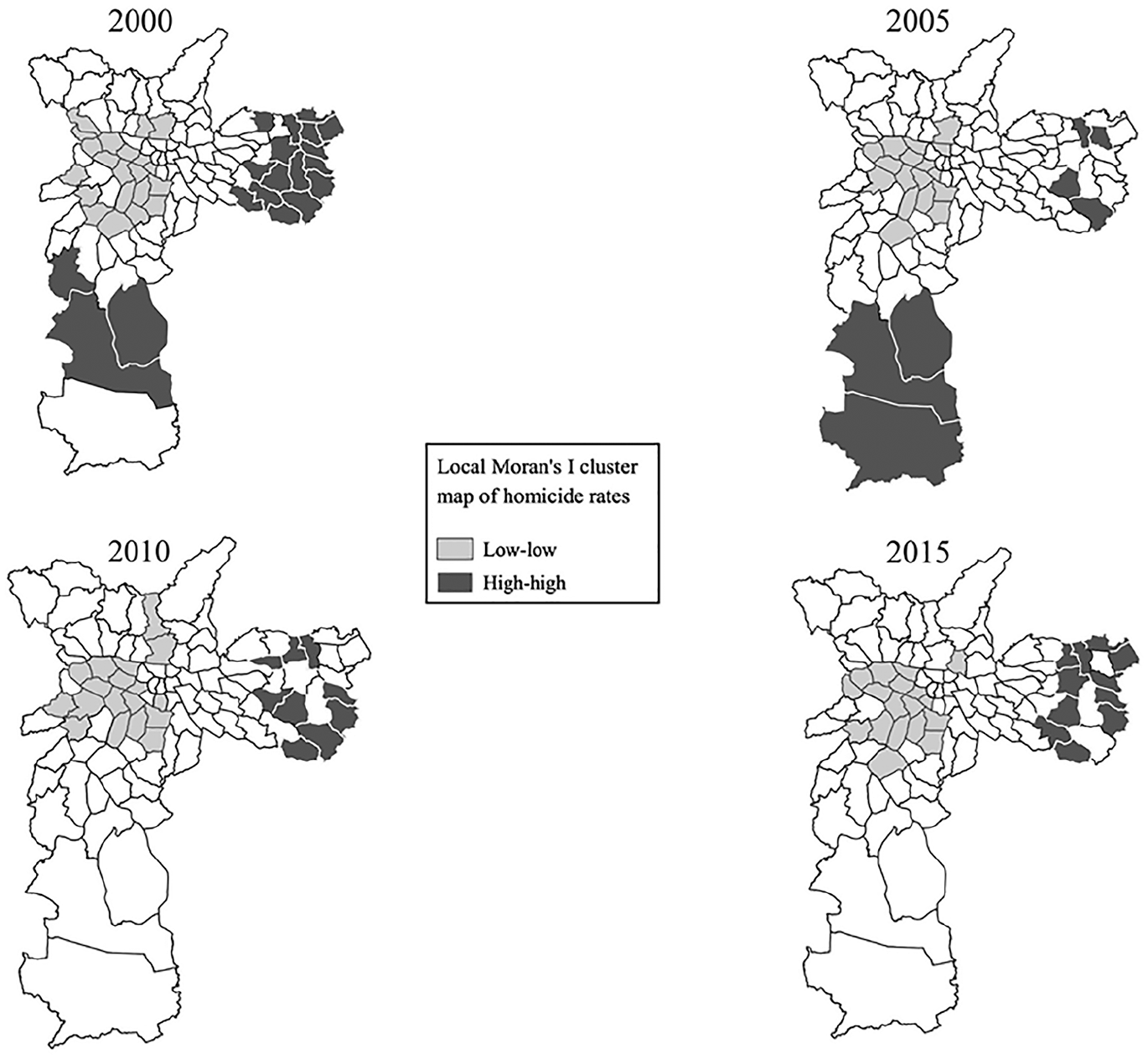
Local Moran’s I cluster map of hot and cool spot (“high-high” or “low-low”) clusters of homicide rates in 96 São Paulo districts (2000, 2005, 2010, 2015).

Figure 4.

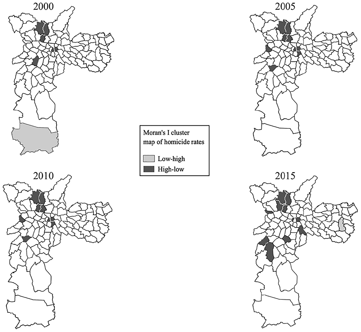
Local Moran’s I cluster map of outlier (“high-low” or “low-high”) clusters of homicide rates in 96 São Paulo districts (2000, 2005, 2010, 2015).

Explaining Temporal Variation in Homicide Rates between Districts

Table 4 displays the spatial panel regression results for Models 1, 2, and 3, which estimate the association between social disorganization and homicide rates, accounting for spatial lag.⁵ The spatial lag coefficients in all models are significant and positive, suggesting that proximity to districts with high homicide is associated with higher homicide rates.⁶ The coefficients for spatial panel models including a spatial lag are not straightforward, as they reflect a combination of indirect and direct effects on homicide rates. Table 4 therefore breaks down the indirect, direct, and total effects of independent variables for each model. The coefficients in Model 1, 2, and 3 in Table 3 were calculated based on the results from Models 1, 2, and 3 in Table 4, respectively. The results for social disorganization in Model 1 show significant direct and indirect (spillover) effects on homicide rates. That is, a one unit (standard deviation) increase in the social disorganization score is associated with an average increase of 0.31 logged homicide rate within the district, and an average increase of 0.21 logged homicide rate in neighboring districts (see Table 5).

Table 4.

Spatial Panel Regression Models of Social Disorganization and Homicide Rate with Random Effects and Spatial Lag.

	Model 1		Model 2		Model 3
Variables	b	SE	b	SE	b	SE
Social disorganization (2000)	0.31***	[0.05]	0.24***	[0.06]
Social disorganization change (Δ2000–2010)					0.73**	[0.27]
Percent youth (15–24)	0.01	[0.01]	0.05	[0.04]	0.03**	[0.01]
Property crime rate per 1,000	0.002*	[0.001]	0.10*	[0.04]	−0.001	[0.001]
Year	0.05	[0.04]	0.05	[0.04]	0.05	[0.04]
Year²	−0.04**	[0.01]	−0.04***	[0.01]	−0.04**	[0.01]
Year³	0.004***	[0.001]	0.005***	[0.001]	0.004**	[0.001]
Year⁴	−0.0001***	[0.00004]	−0.0002***	[0.00004]	−0.0001**	[0.00004]
Social disorganization × year			0.15***	[0.04]
Social disorganization × year²			−0.05***	[0.01]
Social disorganization × year³			0.005***	[0.001]
Social disorganization × year⁴			−0.0001**	[0.00003]
Social disorganization change × year					−0.08	[0.19]
Social disorganization change × year²					0.03	[0.06]
Social disorganization change × year³					−0.004	[0.006]
Social disorganization change × year⁴					0.0001	[0.0001]
Spatial lag	0.41***	[0.05]	0.41***	[0.05]	0.48***	[0.05]
Intercept	1.78***	[0.26]	2.24***	[0.21]	1.39***	[0.26]
σ_u	0.33	[0.03]	0.33	[0.03]	0.38	[1.03]
σ_e	0.45	[0.01]	0.45	[0.01]	0.45	[1.01]
Psuedo R²		0.48		0.48		0.39

Note. SE = standard error; District-level N = 96; District-years N = 1,536.

p < .05. **p < .01. ***p < .001.

Table 5.

Direct, Indirect, and Total Effects for Independent Variables on Homicide Rates.

	Model 1		Model 2		Model 3
	dy/dx	SE	dy/dx	SE	dy/dx	SE
Direct
Social disorganization	0.31***	[0.05]	0.32***	[0.05]
Social disorganization change					0.70**	[0.20]
Percent youth (15–24)	0.12	[0.008]	0.05	[0.04]	0.03**	[0.01]
Property crime rate per 1,000	0.002*	[0.001]	0.10*	[0.04]	−0.001	[0.001]
Indirect
Social disorganization	0.21***	[0.05]	0.19***	[0.05]
Social disorganization change					0.63**	[0.22]
Percent youth (15–24)	0.01	[0.01]	0.03	[0.02]	0.02**	[0.01]
Property crime rate per 1,000	0.001*	[0.001]	0.06*	[0.03]	−0.001	[0.001]
Total
Social disorganization	0.53***	[0.08]	0.51***	[0.08]
Social disorganization change					1.32**	[0.40]
Percent youth (15–24)	0.02	[0.01]	0.09	[0.06]	0.05**	[0.02]
Property crime rate per 1,000	0.003*	[0.001]	0.16*	[0.07]	−0.002	[0.001]

Note. dy/dx reports the average change in logged homicide rate for a one unit change in the independent variable. Estimates were calculated based on Models 1, 2, and 3, respectively from Table 3. SE = standard error.

p < .05. **p < .01. ***p < .001.

Model 2 in Table 4 includes an interaction between district-level social disorganization and time. The results suggest that time trends vary by the level of social disorganization in 2000. In order to better interpret this interaction, we calculated predicted values of the homicide rate by levels of social disorganization (i.e., 1 standard deviation below the mean, mean level, and 1 standard deviation above the mean), holding all other variables at their means. The predicted homicide trajectories are presented in Figure 5. Although the differences are small, Figure 5 shows that districts with lower levels of social disorganization experience earlier and flatter declines closer to a linear shape.

Figure 5.

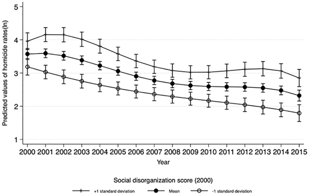
Predicted values and 95% confidence intervals of homicide rates by levels of social disorganization in 2000.

In Model 3 (Table 4), none of the interaction terms are significant, indicating that changes in social disorganization are not associated with differential time trends in homicide rates. Again, we calculated predicted values of the homicide rate by levels of change in social disorganization (i.e., 1 standard deviation below the mean, mean level, and 1 standard deviation above the mean), holding all other variables at their means. The predicted trajectories are presented in Figure 6. In line with the results in Model 3, Table 4, there appears to be no significant differences between trajectories by change in social disorganization. Notably, the coefficient for social disorganization change is positive and significant (b = 0.73, p < .01). In the context of the interaction term, this suggests that an increase in social disorganization is associated with a higher homicide rate at year 0 (2000). Put simply, districts with higher initial homicide rates tended to experience on average increases in social disorganization between 2000 and 2010. These results provide further evidence that the decline in homicide in São Paulo districts cannot be attributed to improvements in socioeconomic conditions.

Figure 6.

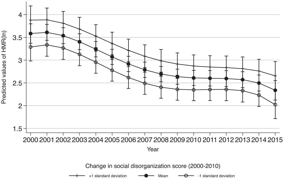
Predicted values and 95% confidence intervals of homicide rates by levels of change in social disorganization (2000–2010).

Discussion and Conclusions

In this study, we explored spatial and temporal patterns of homicide rates and social disorganization in the city of São Paulo. The results showed that there was some degree of uniformity in the decline, whereby all but one district experienced a reduction in homicide rates between 2000 and 2015. However, the pattern and rate of homicide declines varied significantly across districts, suggesting that there is still important variation in the “great São Paulo homicide drop” at smaller units of analysis (De Mello et al., 2010; Goertzel & Kahn, 2009; Peres et al., 2012). Districts with high homicide and social disorganization saw the steepest declines, whereas low-homicide districts saw significantly smaller changes over time. This is further evidenced by the relative temporal instability of “hot spots” compared to “cool spots.” These differential patterns of substantial change in high-homicide and relative stability in low-homicide districts mirrors patterns found in North American cities, which suggest that city-wide crime declines are largely driven by reductions in a small proportion of hot spots (Andresen et al., 2017; Baumer et al., 2018; Wheeler et al., 2016).

Spatial panel models further revealed the spatial interaction between social disorganization and homicide trends in São Paulo districts. Overall, our results are in line with a great deal of quantitative and ethnographic research showing that homicide tends to be highly concentrated in communities characterized by high levels of social and economic disadvantage (Pereira et al., 2017; Peres & Nivette, 2017; Sampson et al., 1997; Valasik et al., 2017; Wickes & Hipp, 2018). Specifically, we found evidence of spatial lag, whereby one district’s homicide rate depends in part on the level of homicide in neighboring districts. Likewise, social disorganization had both a direct association with homicide rates within a district, as well as an indirect, spillover effect on homicide in neighboring districts. This can be interpreted in two ways. First, in line with social disorganization theory, structural disadvantage can breed distrust and weaken social ties and the capacity to enforce norms within a community (Wickes & Hipp, 2018). This distrust, and subsequent consequences, can spread through local networks in a form of contagion diffusion (Cohen & Tita, 1999; Fagan & Davies, 2004). Socially proximate districts (i.e., with high levels of social disorganization) can be more susceptible to these processes (Mears & Bhati, 2006).

Another explanation is that social disorganization opens up the “space” for criminal or organized crime groups to operate in the absence of state authorities (Nivette, 2016). In communities where these groups flourish, criminal activities are not restricted by administrative boundaries, and thus violence perpetrated by these groups may spill over into neighboring districts (Zeoli et al., 2014). According to Adorno and Nery (2019), the PCC riots in May 2006⁷ marked the end of conflicts and revenge cycles among criminal groups in São Paulo, essentially changing the spatial-temporal dynamics of homicide. This could explain the steeper decline and disappearance of high-high clusters in southern São Paulo, an area characterized by an historical concentration of structural disadvantage, very high homicide rates, and strong presence of the PCC (Hirata, 2010). Unfortunately, there is no reliable data on the presence of the PCC at the neighborhood or district level for the entire city of São Paulo. To our knowledge, previous quantitative research has used proxy measures capturing PCC presence in a selection of specific favelas (Biderman et al., 2019), or on the municipal level more broadly (Justus et al., 2018). The contribution of the PCC to the reduction in homicide in São Paulo or, at least in some specific area of São Paulo such as the southern region, requires further investigation.

Importantly, the association between social disorganization and homicide is limited to explaining between-district variation, as we did not find evidence to suggest that changes in social disorganization are associated with variations in homicide rate trajectories. In fact, we found that neighborhood social structural characteristics were largely stable during the period of study (2000–2010). In districts with the highest homicide rates in 2000, social disorganization actually increased marginally, despite experiencing the steepest homicide declines. This casts further doubt on the causal influence of changes in social disorganization on violence in communities, and adds support to the argument that declines in homicide can still be achieved before underlying problems of social disadvantage are solved (Goertzel et al., 2013).

Taken together, the results suggest that other social, economic, or policy changes are responsible for São Paulo’s reversal and decline in homicide. In particular, the broad uniformity of the homicide decline across districts (all but one district experienced an absolute decline in homicide rates between 2000 and 2015) suggests that the underlying drivers of change were experienced to some extent city-wide. Since the late 1990s and early 2000s, there have been several city-wide policy initiatives that could have influenced homicide in São Paulo, including for example conditional cash transfer programs and improvements in policing (Cabral, 2016; Chioda et al., 2015; Freire, 2018; Goertzel & Kahn, 2009; Memória da política de segurança pública de São Paulo, n.d.). Nevertheless, we detected significant heterogeneity in the pattern of homicide decline across districts, whereby highly disorganized communities experienced slightly delayed, less linear declines. If city-level policy initiatives are responsible for homicide declines, there was a certain degree of geographic variation in the timing of implementation or adoption of policies within São Paulo. Districts with high social disorganization characterized by distrust, weakened collective capacity, and a historical lack of state investment and control may have encountered more issues with implementation and acceptance of policy treatments by authorities. Future researchers can exploit these variations in the timing and “dose” of policy treatments across districts to evaluate to what extent policy changes contributed to variations in the decline in homicide rates and hot spots within São Paulo.

It is important to consider that, while our measure of social disorganization includes indicators of disadvantage in line with other research in Latin America (de Melo et al., 2017), the measure is limited in capturing all theoretically important elements of social disadvantage and disorganization processes (e.g., Wickes & Hipp, 2018). Our measure does not include direct indicators of ethnic heterogeneity or residential instability, although these factors are not consistently related to crime and violence in Latin America (e.g., de Melo et al., 2017; Escobar, 2012; Pereira et al., 2017). In particular, our measure is limited to two time points, and thus may not capture more short-term transformations. Given the nearly time-invariant or slow-moving nature of social disorganization, future studies should utilize methods that can more accurately produce reliable within-unit estimates (see Plümper & Troeger, 2007). In addition, analytical techniques such as Geographically Weighted Regression can evaluate the localized, specific effects of social disorganization on homicide rates in each spatial unit (Bernasco & Elffers, 2010). This can allow researchers to explore to what extent characteristics of social disorganization have different effects on homicide rates in different districts across São Paulo.

We also did not measure and test the mediating social processes (e.g., weakened social cohesion, informal social control), and so cannot draw conclusions about which mechanisms are at work. Future research should further examine how different dimensions of social disorganization impact the community’s capacity for collective action, and to what extent alternative agents of social control, such as the PCC, may fill these security gaps (see e.g., Biderman et al., 2019; Justus et al., 2018; Willis, 2015). In addition, given the connection between police killings and homicide in Brazil (Cerqueira, 2012; Soares-Filho et al., 2016), more research is needed to disentangle these two mortality outcomes and evaluate to what extent they might be related over time.

In addition, the size of our unit of analysis (district) may be too large to detect the extent of temporal heterogeneity in homicide trends. The mean population size among districts was 108,608 (SD = 64,468), meaning there is likely within-district heterogeneity in both socio-demographic characteristics and street-level violence trends. Recent studies of crime in micro-places suggests street segments are the ideal unit of analysis to understand the concentration of crime within communities (Baumer et al., 2018; Curman et al., 2015; Wheeler et al., 2016). More localized analyses of spatial and temporal homicide trends may be able to better disentangle the complex macro- and micro-level factors that contributed to the homicide decline in São Paulo.

Footnotes

Appendix A

Table A1.

Multilevel Linear Regression Models for Homicide Mortality Rate, Identifying the Best Fit Time Trend.

	Model 1		Model 2		Model 3		Model 4		Model 5		Model 6		Model 7		Model 8
Variables	b	SE	b	SE	b	SE	b	SE	b	SE	b	SE	b	SE	b	SE
Year			−0.09***	[0.003]	−0.09***	[0.002]	−0.09***	[0.003]	−0.16***	[0.01]	−0.11***	[0.02]	0.09**	[0.03]	0.06	[0.05]
Year²									0.004***	[0.001]	−0.003	[0.002]	−0.07***	[0.01]	−0.06*	[0.02]
Year³											0.0003	[0.0001]	0.01***	[0.001]	0.005	[0.004]
Year⁴													−0.0003***	[0.00003]	−0.00004	[0.0003]
															−0.000006	[0.000008]
Intercept	2.88***	[0.05]	3.53***	[0.06]	3.56***	[0.06]	3.57***	[0.06]	3.68***	[0.06]	3.65***	[0.07]	3.55***	[0.07]	3.55***	[0.07]
Intercept variance	0.25	[0.04]	0.26	[0.04]	0.28	[0.04]	0.35	[0.05]	0.35	[0.06]	0.35	[0.05]	0.35	[0.05]	0.35	[0.05]
L1 variance							0.0004	[0.0001]	0.0004	[0.0001]	0.0005	[0.0001]	0.0004	[0.0001]	0.0004	[0.0001]
Cov (intercept, L1 slope)							−0.01*	[0.002]	−0.01	[0.002]	−0.01	[0.002]	−0.01	[0.002]	−0.01	[0.002]
Model	Constant, random intercept		Linear, random intercept		Linear, random intercept, unstructured covariance		Linear, random intercept, random slope, unstructured covariance		Quadratic, random intercept, random slope, unstructured covariance		Cubic, random intercept, random slope, unstructured covariance		Quartic, random intercept, random slope, unstructured covariance		Quintic, random intercept, random slope, unstructured covariance
Log likelihood	−1575.91		−1163.20		−1036.55		−1023.58		−992.35		−989.59		−963.80		−963.55
Likelihood ratio test			M1 versus M2 X²(1 df): 825.42***		M2 versus M3 X²(15 df): 253.32***		M3 versus M4 X²(2 df): 25.93***		M4 versus M5 X²(1 df): 62.47***		M5 versus M6 X²(1 df): 5.52*		M6 versus M7 X²(1 df): 51.57***		M7 versus M8 X²(1 df): 0.49

Note. SE = standard error; District-level N = 96; District-years N = 1,536.

p < .05. **p < .01. ***p < .001.

Declaration of Conflicting Interests

The author(s) declared no potential conflicts of interest with respect to the research, authorship, and/or publication of this article.

Funding

The author(s) disclosed receipt of the following financial support for the research, authorship, and/or publication of this article: This project is funded by The Brazilian National Council for Scientific and Technological Development (Award number: 423550/2016-0).

ORCID iD

Amy Nivette

Notes

Author Biographies

Amy Nivette is an associate professor of sociology at Utrecht University. Her research interests include the determinants and effects of institutional legitimacy and attitudes toward the law, the comparative study of aggression and violence, and violent extremism.

Maria Fernanda Tourinho Peres is a medical doctor with a PhD in Public Health. She is professor at the Preventive Medicine Department at the Medical School of the University of São Paulo, Brazil, member of the Violence Prevention Alliance and coordinator of the Laboratório Interdisciplinar de Estudos Sobre Violência e Saúde (LIEVES).

References

Adorno

Nery

(2019). Crime e violências em São Paulo: retrospectiva teórico-metodológica, avanços, limites e perspectivas futuras. Cadernos Metropóle, 21(44): 169–194.

Adorno

Salla

(2007). Criminalidade organizada nas prisões e os ataques do PCC. Estudos Avançados, 21(61): 7–29.

Andresen

M. A.

Curman

A. S.

Linning

S. J.

(2017). The trajectories of crime at places: understanding the patterns of disaggregated crime types. Journal of Quantitative Criminology, 33, 427–449.

Anselin

(2013). Spatial econometrics: methods and models. Kluwer.

Anselin

(1999). Interactive techniques and exploratory spatial data analysis. In Longley

P. A.

Goodchild

M. F.

Maguire

D. J.

Rhind

D. W.

(Eds.), Geographic information systems: Principles, techniques, management and applications (pp. 251–264). Wiley.

Anselin

(1995). Local indicators of spatial autocorrelation–LISA. Geographical Analysis, 27, 93–115.

Baller

R. D.

Anselin

Messner

S. F.

Deane

Hawkins

D. F.

(2001). Structural covariates of U.S. county homicide rates: Incorporating spatial effects. Criminology, 39, 561–590.

Baumer

E. P.

Velez

M. B.

Rosenfeld

(2018). Bringing crime trends back into criminology: A critical assessment of the literature and a blueprint for future inquiry. Annual Review of Criminology, 1, 39–61.

Baumer

E. P.

Wolff

K. T.

(2014). Evaluating contemporary crime drops in America, New York City, and many other places. Justice Quarterly, 31, 5–38.

10.

Biderman

De Mello

J. M. P.

De Lima

R. S.

Schneider

(2019). Pax Monopolista and crime: The case of the emergence of the Primeiro Comando da Capital in São Paulo. Journal of Quantitative Criminology, 35, 573–605.

11.

Bernasco

Elffers

(2010). Statistical analysis of spatial crime data. In Piquero

A. R.

Weisburd

(Eds.), Handbook of quantitative criminology (pp. 699–724). Springer.

12.

Breetzke

G. D.

(2010). Modeling violent crime rates: A test of social disorganization in the city of Tshwane, South Africa. Journal of Criminal Justice, 38, 446–452.

13.

Cabral

M. V.

(2016). Avaliação do impacto do INFOCRIM sobre as taxas de homicídios dos municípios paulistas: uma aplicação do método das diferenças em diferenças espacial [PhD dissertation]. Juiz de Fora, Brazil: Universidade Federal de Juiz de Fora.

14.

Cámara de Comercio de Bogotá. (2015). Protocolo de Bogotá: sobre calidad de los datos de homicidio en América Latina y el Caribe. https://www.ccb.org.co/Sala-de-prensa/Noticias-CCB/2015/Noviembre-2015/Protocolo-de-Bogota-sobre-calidad-de-los-datos-de-homicidios-en-America-Latina-y-el-Caribe

15.

Cardia

Adorno

Poleto

F. Z.

(2003). Homicide rates and human rights violations in São Paulo, Brazil: 1990 to 2002. Health and Human Rights, 6, 14–33.

16.

Ceccato

Haining

Kahn

(2007). The geography of homicide in São Paulo, Brazil. Environment and Planning A, 39, 1632–1653.

17.

Ceccato

Oberwittler

(2008). Comparing spatial patterns of robbery: Evidence from a Western and an Eastern European City. Cities, 25, 185–196.

18.

Cerdá

Morenoff

J. D.

Hansen

B. B.

Hicks

K. J. T.

Duque

L. F.

Restrepo

Diez-Roux

A. V.

(2012). Reducing violence by transforming neighborhoods: A natural experiment in Medellín, Colombia. American Journal of Epidemiology, 175, 1045–1053.

19.

Cerqueira

(2012). Mortes violentas não esclarecidas e impunidade no Rio de Janeiro. Economia Aplicada, 16, 201–235.

20.

Chioda

De Mello

J. M. P.

Soares

R. R.

(2015). Spillovers from conditional cash transfer programs: Bolsa Família and crime in Urban Brazil. Econonmics of Education Review, 54, 306–320.

21.

Cohen

Tita

(1999). Diffusion in homicide: Exploring a general method for detecting spatial diffusion processes. Journal of Quantitative Criminology, 15, 451–493.

22.

Curman

A. S. N.

Andresen

M. A

Brantingham

P. J.

(2015). Crime and place: A longitudinal examination of street segment patterns in Vancouver, BC. Journal of Quantitative Criminology, 31, 127–147.

23.

de Melo

S. N.

Andresen

M. A.

Matias

L. F

. (2017). Geography of crime in a Brazilian context: An application of social disorganization theory. Urban Geography, 38, 1550–1572.

24.

De Mello

J. M. P.

Schneider

. (2010). Assessing São Paulo’s large drop in homicides: The role of demography and policy interventions. In Di Tella

Edwards

Schargrodsky

(Eds.), The economics of crime: Lessons for and from Latin America (pp. 207–235). University of Chicago Press.

25.

Dias

C. C. N.

(2009). Ocupando as brechas do Direito formal: o PCC como instância alternativa de resolução de conflitos. Dilemas: Revista de Estudos de Conflito e Controle Social, 2(4): 83–105.

26.

Dias

C. C. N.

(2013). PCC: Hegemonia nas prisões e monopólio da violência. Saraiva.

27.

Elhorst

J. P.

(2014). Spatial econometrics: From cross-sectional data to spatial panels. Springer.

28.

Escobar

(2012). El uso de la teoría de la desorganización social para comprender la distribución de homicidios en Bogotá, Colombia. Revista INVI, 27, 21–85.

29.

Fagan

Davies

(2004). The natural history of neighborhood violence. Journal of Contemporary Criminal Justice, 20, 127–147.

30.

Farrell

Tilley

Tseloni

Mailley

(2010). Explaining and sustaining the crime drop: Clarifying the role of opportunity-related theories. Crime Prevention and Community Safety, 12(1), 24–41.

31.

Feltran

G. S.

(2010). Crime e castigo na cidade: os repertórios da justice e a questão do homicídio nas periferias de São Paulo. Caderno CRH, 23(58): 59–73.

32.

Fórum Brasileiro de Segurança Pública. (2016). Projeto: Pesquisa e análise de dados vinculandos ao campo da segurança pública e sistema penitenciário. Termo de Parceria No. 817052/2015. https://forumseguranca.org.br/storage/publicacoes/FBSP_Estudo_classificacoes_estatisticas_tipificacoes_penais_2016.pdf

33.

Freire

(2018). Evaluating the effect of homicide prevention strategies in São Paulo, Brazil: A synthetic control approach. Latin American Research Review, 53, 231–249.

34.

Goertzel

Kahn

(2009). The great Sao Paulo homicide drop. Homicide Studies, 13, 398–410.

35.

Goertzel

Shohat

Kahn

Zanetic

Bogoyavlenskiy

(2013). Homicide booms and busts: A small-n comparative historical study. Homicide Studies, 17, 59–74.

36.

Griffiths

(2013). Race, space, and the spread of violence across the city. Social Problems, 60, 491–512.

37.

Hipp

J. R.

Wickes

(2017). Violence in urban neighborhoods: A longitudinal study of collective efficacy and violent crime. Journal of Quantitative Criminology, 33, 783–808.

38.

Hirata

D. V.

(2010). Sobreviver ba adversidade: entre o mercado e a vida. Tese de Doutorado em Sociologia. Faculdade de Filosofia, Letras e Ciências Humanas, Universidade de São Paulo. https://www.teses.usp.br/teses/disponiveis/8/8132/tde-03032011-122251/publico/2010_DanielVelosoHirata.pdf

39.

Ingram

M. C.

da Costa

M. M.

(2017). A spatial analysis of homicide across Brazil’s municipalities. Homicide Studies, 21, 87–110.

40.

Instituto Brasileiro de Geografia e Estatística. (n.d.). Brazil: Instituto Brasileiro de Geografia e Estatística. https://sidra.ibge.gov.br

41.

Justus

de Castro Cerqueira

D. R.

Kahn

Moreira

G. C.

(2018). The “São Paulo Mystery”: The role of the criminal organization PCC in reducing the homicide in 2000s. EconomiA, 19, 201–218.

42.

Kawachi

Kennedy

B. P.

Wilkinson

R. G.

(1999). Crime: Social disorganization and relative deprivation. Social Science & Medicine, 48, 719–731.

43.

Kikuchi

Desmond

S. A.

(2010). A longitudinal analysis of neighborhood crime rates using latent growth curve modeling. Sociological Perspectives, 53, 127–149.

44.

Light

M. T.

Harris

C. T.

(2012). Race, space, and violence: Exploring spatial dependence in structural covariates of white and black violent crimes in US counties. Journal of Quantitative Criminology, 28, 559–586.

45.

Loeffler

Flaxman

(2018). Is gun violence contagious? A spatiotemporal test. Journal of Quantitative Criminology, 34, 999–1017.

46.

Martinez

Jr. Stowell

J. I.

Lee

M. T.

(2010). Immigration and crime in an era of transformation: A longitudinal analysis of homicides in San Diego neighborhoods, 1980-2000. Criminology, 48, 797–829.

47.

McCall

P. L.

Land

K. C.

Parker

K. F.

(2010). An empirical assessment of what we know about structural covariates of homicide rates: A return to a classic 20 years later. Homicide Studies, 14, 219–243.

48.

Mears

D. P.

Bhati

A. S.

(2006). No community is an island: The effects of resource deprivation on urban violence in spatially and socially proximate communities. Criminology, 44, 509–548.

49.

Memória da política de segurança pública de São Paulo. (n.d.). São Paulo: Fórum Brasileiro de Segurança Pública and Instituto Betty e Jacob Laffer. https://memoria.forumseguranca.org.br/infografico/

50.

Messner

S. F.

Anselin

Baller

R. D.

Hawkins

D. F.

Deane

Tolnay

S. E.

(1999). The spatial patterning of county homicide rates: An application of exploratory spatial data analysis. Journal of Quantitative Criminology, 15, 423–450.

51.

Morenoff

J. D.

Sampson

R. J.

Raudenbush

S. W.

(2001). Neighborhood inequality, collective efficacy, and the spatial dynamics of urban violence. Criminology, 39, 517–560.

52.

Muggah

Szabó

Carvalho

Alvarado

Marmolejo

Wang

(2016). Making cities safer: Citizen security innovations from Latin America. Inter-American Development Bank Strategic Paper 20. https://publications.iadb.org/en/making-cities-safer-citizen-security-innovations-latin-america

53.

Nivette

A. E.

(2016). Institutional ineffectiveness, illegitimacy, and public support for vigilantism in Latin America. Criminology, 54,142–175.

54.

Oliveira

Silva

B. F. A.

Prates

M. O.

(2015). Street drug markets beyond favelas in Belo Horizonte, Brazil. Crime Science, 4, 1–11.

55.

Osorio

(2015). The contagion of drug violence: Spatiotemporal dynamics of the Mexican War on Drugs. Journal of Conflict Resolution, 59, 1403–1432.

56.

Pereira

D. V.

Mota

C. M.

Andresen

M. A.

(2017). Social disorganization and homicide in Recife, Brazil. International Journal of Offender Therapy and Comparative Criminology, 61, 1570–1592.

57.

Peres

M. F. T.

de Almeida

J. F.

Vincentin

Ruotti

Nery

M. B.

Cerda

Cardia

Adorno

(2012). Homicide and public security indicator trends in the city of Sao Paulo between 1996 and 2008: a time-series ecological study. Ciência & Saúde Coletiva, 17, 3249–3257.

58.

Peres

M. F. T.

Nivette

A. E.

(2017). Social disorganization and homicide mortality rate trajectories in Brazil between 1991 and 2010. Social Science & Medicine, 190, 92–100.

59.

Perlman

J. E.

(2006). The metamorphosis of marginality: Four generations in the favelas of Rio de Janeiro. Annals of the American Academy of Political and Social Science, 606, 154–177.

60.

Plümper

Troeger

V. E.

(2007). Efficient estimation of time-invariant and rarely changing variables in finite sample panel analyses with unit fixed effects. Political Analysis, 15(2), 124–139.

61.

Rabe-Hasketh

Skrondal

(2012). Multilevel and longitudinal modeling using Stata: Volume 1: Continuous responses. Stata Press.

62.

Raudenbush

S. W.

Bryk

A. S.

(2002). Hierarchical linear models: Applications and data analysis methods. Sage.

63.

Rengert

G. F.

Ratcliffe

J. H.

Chakravorty

(2005). Policing illegal drug markets: Geographic approaches to crime reduction. Criminal Justice Press.

64.

Sampson

R. J.

Groves

W. B.

(1989). Community structure and crime: Testing social-disorganization theory. American Journal of Sociology, 94, 774–802.

65.

Sampson

R. J.

Morenoff

J. D.

(2006). Durable inequality: Spatial dynamics, social processes, and the persistence of poverty in Chicago neighborhoods. In Bowles

Durlauf

S. N.

Hoff

(Eds.), Poverty traps (pp. 176–203). Princeton University Press.

66.

Sampson

R. J.

Raudenbush

S. W.

Earls

(1997). Neighborhoods and violent crime: A multilevel study of collective efficacy. Science, 277, 918–925.

67.

Secretaria Municipal de Saúde. Prefeitura do Município de São Paulo (n.d.). São Paulo: Prefeitura do Município de São Paulo. https://www.prefeitura.sp.gov.br/cidade/secretarias/saude/tabnet/

68.

Shaw

McKay

H. D.

(1942). Juvenile delinquency and urban areas. University of Chicago Press.

69.

Soares-Filho

A. M.

Cortez-Escalante

J. J.

França

(2016). Revisão dos métodos de correcto de óbitos e dimensões de qualidade da causa básica por acidentes e violências no Brasil. Ciência & Saúde Colteiva, 21, 3803–3818.

70.

StataCorp. (2019). Stata Statistical Software: Release 16. StataCorp LLC.

71.

Steenbeek

Hipp

J. R.

(2011). A longitudinal test of social disorganization theory: feedback effects among social cohesion, social control, and disorder. Criminology, 49, 833–871.

72.

Stults

B. J.

(2010). Determinants of Chicago neighborhood homicide trajectories: 1965-1995. Homicide Studies, 14, 244–267.

73.

Tita

G. E.

Radil

S. M.

(2010). Spatial regression models in criminology: Modeling social processes in the spatial weights matrix. In Piquero

A. R.

Weisburd

(Eds.), Handbook of quantitative criminology (pp. 101–121). Springer.

74.

Tuttle

McCall

P. L.

Land

K C.

(2018). Latent trajectories of cross-national homicide trends: structural characteristics of underlying groups. Homicide Studies, 22(4), 343–369. https://doi.org/10.1177/1088767918774083

75.

Unger

Riley

L. W.

(2007). Slum health: From understanding to action. PLoS Medicine, 4, 1561–1566.

76.

Valasik

Barton

M. S.

Reid

S. E.

Tita

G. E.

(2017). Barriocide: Investigating the temporal and spatial influence of neighborhood structural characteristics on gang and non-gang homicides in East Los Angeles. Homicide Studies, 21, 287–311.

77.

Vilalta

Muggah

(2014). Violent disorder in Ciudad Juarez: A spatial analysis of homicide. Trends in Organized Crime, 17, 161–180.

78.

Villarreal

Silva

B. F.

(2006). Social cohesion, criminal victimization and perceived risk of crime in Brazilian neighborhoods. Social Forces, 84, 1725–1753.

79.

Wheeler

A. P.

Worden

R. E.

McLean

S. J.

(2016). Replicating group-based trajectory models of crime at micro-places in Albany, NY. Journal of Quantitative Criminology, 32, 589–612.

80.

Wickes

Hipp

J. R.

(2018). The spatial and temporal dynamics of neighborhood informal social control and crime. Social Forces, 97, 277–308.

81.

Willis

G. D.

(2015). The killing consensus: Police, organized crime, and the regulation of life and death in Urban Brazil. University of California Press.

82.

(2011). Analyzing the dynamics of homicide patterns in Chicago: ESDA and spatial panel approaches. Applied Geography, 31, 800–807.

83.

Zeoli

A. M.

Pizarro

J. M.

Grady

S. C.

Melde

(2014). Homicide as infectious disease: Using public health methods to investigate the diffusion of homicide. Justice Quarterly, 31, 609–632.

Social Disorganization and Urban Homicide Rates: A Spatial-Temporal Analysis in São Paulo,Brazil 2000 to 2015

Abstract

Keywords

Social Disorganization and Homicide Rates

The Current Study

Methods

Data and Measures

Statistical Analyses

Results

Descriptive Statistics

Temporal Variation in Homicide Rates

Spatial Variation in Homicide Rates

Explaining Temporal Variation in Homicide Rates between Districts

Discussion and Conclusions

Footnotes

Appendix A

Declaration of Conflicting Interests

Funding

ORCID iD

Notes

Author Biographies

References