
Abstract
Disordered biopolymer gels, such as alginate gels, contain disordered amorphous regions as well as ordered regions known as junction zones, the latter playing a paramount role in maintaining the integrity of the gel network. The considerable dimensions of these junction zones and their physical interactions are responsible for distinctive phenomena, such as self-healing, observed in biopolymer gels. Compared to rubber-like materials, where polymer chains are interconnected by chemical cross-links, statistical mechanics modeling of disordered biopolymer gels poses new challenges due to the need to capture the contributions from both the disordered and ordered regions. In the literature, the disordered domains are usually modeled by a collection of random coils, while each junction zone is represented by a rigid rod. Attempt has been made to introduce the two-node coil-rod structure, consisting of a random coil connected to a rigid rod, into classical polymer network models (e.g., the Arruda–Boyce eight-chain model) to predict the mechanical response of the biopolymer gels. Although this approach provides valuable insights and reasonable predictions that agree with experimental data, the interactions between the junction zones and the amorphous regions are significantly simplified. This study aims to extend the two-node coil-rod structure to a four-node coil-rod structure, in which two polymer chains share a junction zone, more explicitly representing chain association induced by physical forces in biopolymer gels. By incorporating statistical mechanics and the phantom network model, the entropy of the system is derived, from which the stress–stretch relationships for the network are obtained. Comparisons are made with the model based on the two-node coil-rod structure, and the conditions for establishing equivalency between the two methods are examined. This work establishes a foundation for developing more advanced network models that incorporates the simultaneous interaction of multiple junction zones, a phenomenon often present in biopolymer gels.
Keywords
Nomenclature
1. Introduction
Polymer networks are established through the copious interpenetration of chains. The complex interactions between them as well as structural features such as topological loops [1] make studying their statistical thermodynamics formidable. In the method proposed by James and Guth [2,3], known as the affine network model, the chain vectors are situated randomly within the network, and their extension is assumed to follow the macroscopic deformation controlled by external loading. In this framework, since the interaction of chains are only considered via cross-links, the partition function of each chain provides sufficient information to obtain the partition function of the entire network. Building upon this pioneering work, subsequent literature endeavors to develop more advanced models that describe observed phenomena in polymer networks while being numerically affordable. To name but a few, these includes the three-chain model [4], the full-network model [5,6], the eight-chain model [7,8], and the micro-sphere model [9]. In the method proposed by Flory [10], known as the phantom network model, the constraints of macroscopic deformation are relaxed, allowing the chains to maintain their topology while freely passing through each other. In this framework, the network is treated as a collection of chains where only a subset of cross-links is restricted by macroscopic deformation, while the remaining cross-links fluctuate around their average positions.
In disordered biopolymer gels, amorphous regions known as coils are interconnected through ordered regions called junction zones [11,12]. The process of junction zone formation varies depending on the specific biopolymers involved. For instance, in agar gels, the chains intertwine to create a double helix structure, while in alginate gels, the junction zone is formed through the mediation of external cation agents, resulting in egg-box structures. Disordered biopolymer gels can be decomposed into two fundamental building blocks: coils and junction zones. Coils are often modeled as freely jointed chains, while junction zones are represented by rigid rods. Within the framework of affine network, the end-to-end extension of each component (coil or rod) is assumed to be proportional to the corresponding macroscopic displacement. Since the rigid rod has infinite stiffness and therefore cannot undergo extension, the macroscopic behavior encompassing the rod reflects an unrealistically high stiffness under affinity assumptions.
To mitigate this issue, Higgs and Ball [13], and later Moosavian and Tang [14], considered the network as a collection of “coil-rod” structures, in each structure the freely jointed chain is connected to a rigid rod (see Figure 1(a)). The end-to-end extension of this combined structure (rather than treating the coil and rod separately) still follows the macroscopic deformation akin to an affine network. However, the node connecting the coil and rod can freely move resembling the phantom network. Since the macroscopic deformation can be related to the distance between two end nodes of the structure, it is hereafter referred to as the “two-node coil-rod structure”. This structure can be directly integrated into well-known affine network models in the literature. In addition, it allows us to capture the phenomenon of zipping/unzipping, where the junction zones expand or shrink due to applied loading. Recently, it has been demonstrated that implementing the two-node coil-rod structure with zipping/unzipping into the eight-chain model effectively captures both the dissipation caused by unzipping and the phenomenon of permanent set observed during cyclic loading and unloading [15]. Despite these advances, the two-node coil-rod structure in the aforementioned model is treated as a single entity. The decomposition of the complicated network, involving different regions of coils and rods, into a collection of two-node coil-rod structures is a simplification worth further examination. This prompts us to advance the model into a more explicit network where two or more coils are connected by sharing a single junction zone in the middle (see Figure 1(b)). Such a representation takes steps toward a more accurate depiction of chain interactions in biopolymer gels. By providing the new model, the ranges of applicability and limitations of the two-node coil-rod structure can also be explored, addressing whether it can adequately model the complex interactions between coils and rods.
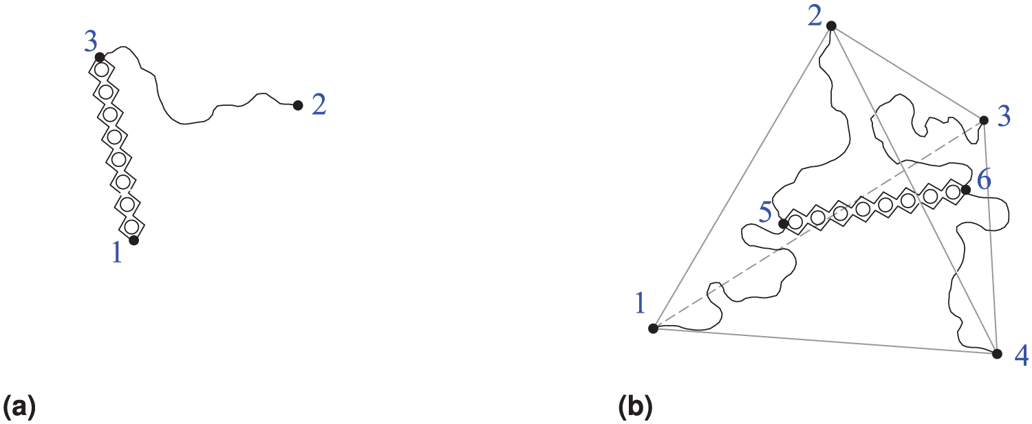
(a) The two-node coil-rod structure with nodes 1 and 2 attached to the macroscopic network and fluctuating node 3. The zigzag drawing is a schematic representation of the egg-box structure, with hollow circles indicating the gelling agents. Segment between 1 and 3 is modelled by a rigid rod and the coil between 2 and 3 is modelled by freely jointed chain. (b) The topology of the four-node coil-rod structure with nodes 1 to 4 attached to the macroscopic network and fluctuating nodes 5 and 6. The zigzag structure between 5 and 6 represents the rigid rod and the remaining four coils follow the freely jointed chain model.
In Section 2, the model of the two-node coil-rod structure is briefly reviewed, and a new four-node coil-rod structure is formulated within the framework of statistical mechanics in Section 2.1. Two formalisms for deriving the probability distribution are explained in Sections 2.2 and 2.3. Subsequently, the results are simplified by invoking Gaussian statistics for the coils in Section 2.4. It is shown that under this assumption, the four-node coil-rod structure can be decomposed into a collection of one two-node coil-rod structure and two pure coils. Section 3 integrates this finding into network models, and the results are compared with the eight-chain network model containing two-node coil-rod structures. Finally, Section 4 discusses the limitations and advantages of the proposed model for further applications.
2. Statistical mechanics of a four-node coil-rod structure
Prior to developing the four-node coil-rod structure, the formulation of a two-node coil-rod structure is reviewed. For a freely jointed chain with Kuhn length b and number of Kuhn segments n, if the end-to-end distance

where

where

The superscripts CR, R, and C, respectively, signifies the two-node coil-rod, rod, and coil structure. For
2.1. Four-node coil-rod structure
The simplest scenario illustrating the explicit interaction of coils and rods involves two coils sharing a single junction zone between them. Let us consider two coils, labeled 13 and 24 in Figure 1(b), which are laterally associated, thereby creating the junction zone 56 and regenerating four new coils 15, 25, 36, and 46. In three-dimensional space, the four nodes can form a cell as demonstrated by a tetrahedral in Figure 1(b). Hereafter, such a structure is referred to as the “four-node coil-rod structure”.
By defining

where ϱ is the chain density per unit reference volume,

where T is the absolute temperature. Depending on the geometry of four-node coil-rod structure, the dimensions

It can be seen that the constitutive equation directly depends on the probability distribution
2.2. Real space representation of the probability
Suppose the probability distribution for a coil with
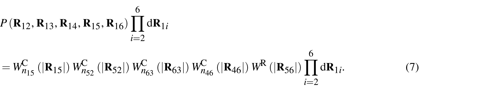
Now, the probability of finding nodes 2 to 4 within their own volume elements
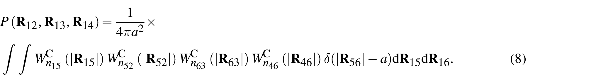
By employing the following change of variables


equation (8) is rephrased as
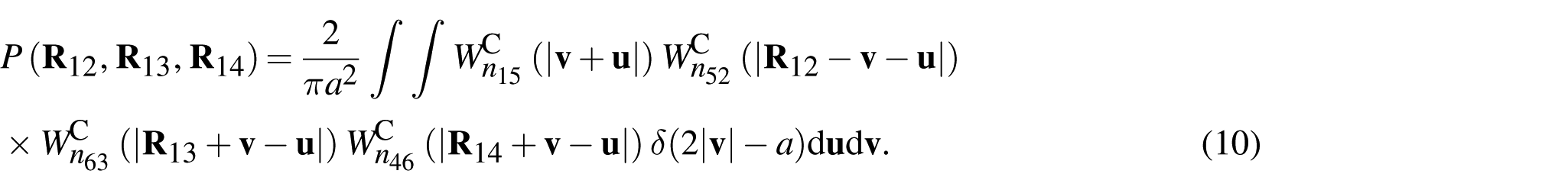
Utilizing
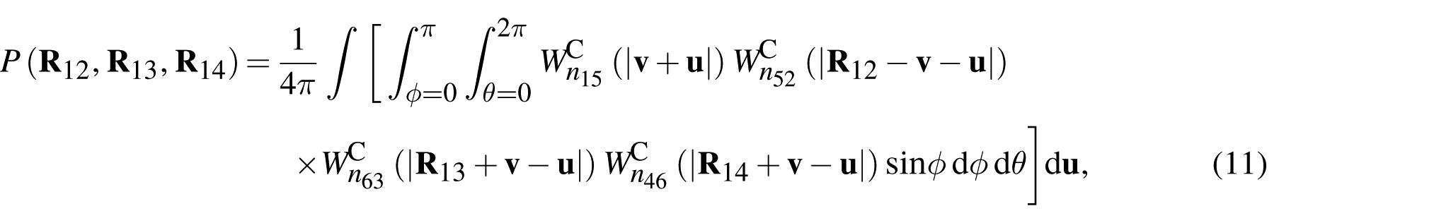
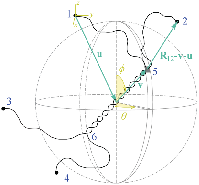
where

The schematics of the above variables are illustrated in Figure 2. It should be recalled that in freely jointed chain models, coils cannot extend beyond their fully extended state, where the associated probability is zero. Analogously, the maximum value of
The five layers of integration in equation (11) include three-dimensional integration over all possible vectors
In the context of more complex system of coils and rods, the number of integration layers is given by
2.3. Fourier space representation of the probability
Fourier space representation sometimes offers a simpler approach to calculating the probability distribution. Since nodes 1 to 4 are attached to the macroscopic element, the following constraints between the end-to-end vectors hold:


Now, the probability (8) is restated as follows:
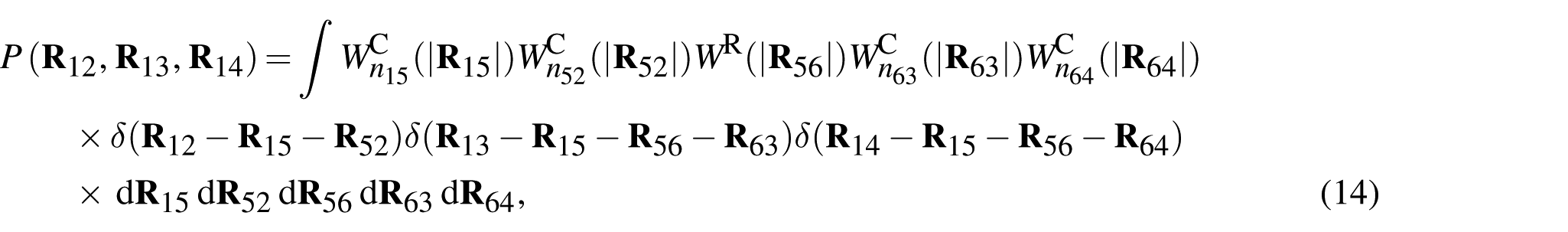
where the constraints (13) are enforced through three-dimensional Dirac delta functions

where
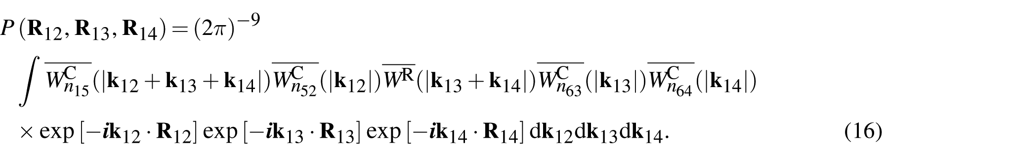
In (16), the bar over a symbol denotes the Fourier transform of the function defined as:

For the rigid rod with length a, the Fourier transform of equation (2) gives rise to

2.4. Gaussian coil approximation
Thus far, the probability distribution has been expressed in the form of multi-variable integrations, involving a substantial numerical burden. In this section, it will be shown that Gaussian approximation of coils can significantly simplify the calculations.
The probability distribution function of the Gaussian phantom network (with no rods) has been obtained by Flory [10] using real space representation. In Appendix 1, the same network is formulated with the aid of Fourier transform and it is shown that the result has an analytical closed form. Likewise, the integration described in (16) can be simplified by assuming a Gaussian distribution for coils 15, 52, 63, and 46. Suppose that

Let us represent the vectors


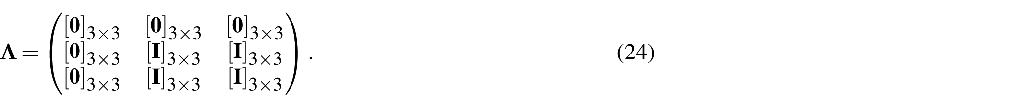
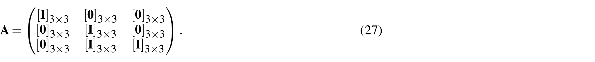
Now, by defining the matrices


with label T denotes the transpose of the matrix, the integration (16) is rephrased as the following compact form:

where
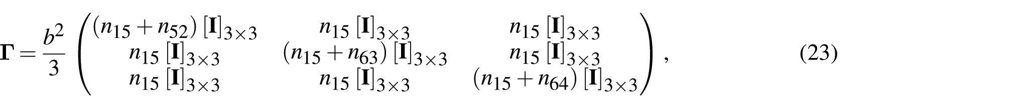
and
In the above relations,

where


and
Since

where

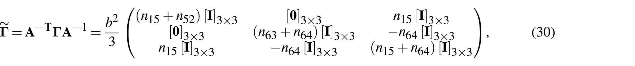
and

Label
in which


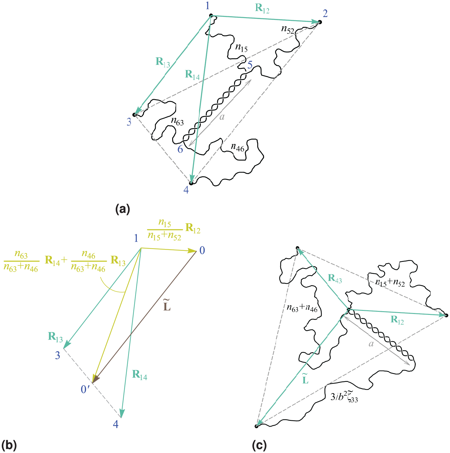
(a) The topology of the four-node coil-rod structure with rod length a and corresponding end-to-end vectors
The probability distribution of the four-node coil-rod structure can be generalized to (

The above representation not only makes the notation simpler but also lays the solid base for comparing the present models with models in the literature based on two-node coil-rod structure and pure coils. Now suppose that the chains 15 and 52, as well as chains 63 and 46 are identical such that


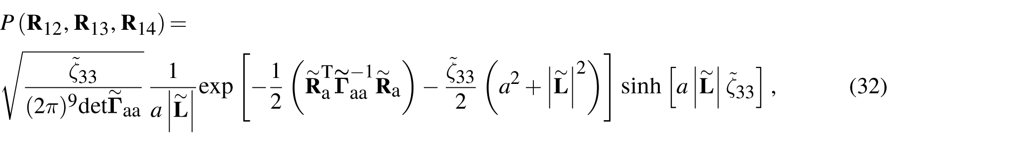
Therefore, equation (34) is rewritten as

3. Implementation into network
As mentioned earlier, once the probability distribution is established, the mechanical response of the gel can be determined by placing the four-node coil-rod structure within a macroscopic network with specific geometry. In this manner, the macroscopic deformation can be properly translated to the constituent structure. To examine the features of the four-node coil-rod structure, a simple scenario is first considered where the four nodes are placed in the same plane in the form of a rectangular cell as seen in Figure 4(a). It should be noted that while the nodes form a two-dimensional cell, the chains can occupy the three-dimensional space.
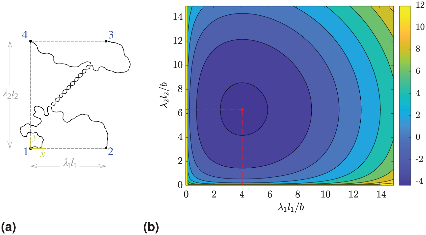
(a) A four-node coil-rod structure with the four nodes placed in the same plane in a rectangular manner with deformed dimensions
3.1. In-plane placement of four nodes
Referring to Figure 4(a), suppose the nodes 1 to 4 are initially positioned at the vertices of a rectangle with edge lengths of

where setting

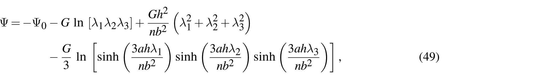
Now, by substitution of equation (38) into equations (4) and (5), the Helmholtz free energy can be calculated as follows:

in which


The distinct stress–stretch relationship in each principal direction demonstrates the intrinsic anisotropy of the four-node coil-rod structure shown in Figure 4(a). The above stress components can be set to zero for


Equation (42b) is an implicit function of a and typically requires numerical computations. However, for

In this case, as

holds for
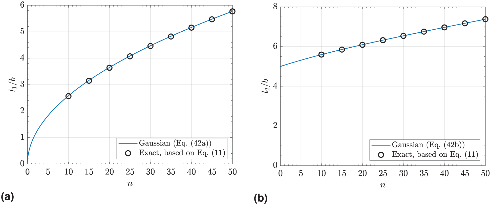
As it was alluded to, the applicability of Gaussian coils in the freely jointed chain model is constrained to small extensions of the coils and a large number of Kuhn segments. To assess the validity of such approximation in determining

with

and
(a)
Next, the accuracy of the constitutive relations (40) and (41) is validated against the exact result without the Gaussian approximation. As mentioned earlier, after calculation of the exact Helmholtz free energy via equations (11), (4), (5), and (45), the stress components can be determined through equation (6). Since the numerical burden of evaluating (11) is heavy, the biaxial test is preferred over the uniaxial test. In the biaxial test,
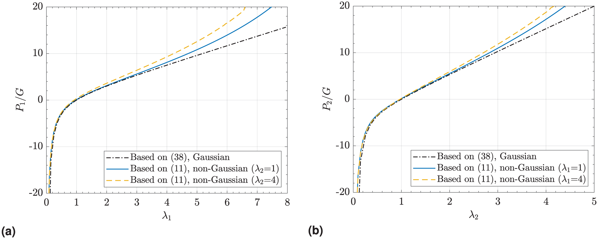
The normalized principal stress vs. the principal stretch for biaxial test and
3.2. Extension to 3D
Based on the formulation in Section 3.1, the four-node coil-rod structure shown in Figure 4(a) can be incorporated into the three-dimensional network to account for more general deformation states. One example is shown in Figure 7, where identical four-node coil-rod structures are placed, with different orientations, on three faces of the rectangular prism: 1234, 1265, and 1485. Suppose that the principal stretches are aligned with the prism edges. The arrangement of the four-node coil-rod structures is such that the prism has a cube shape with edge length h when

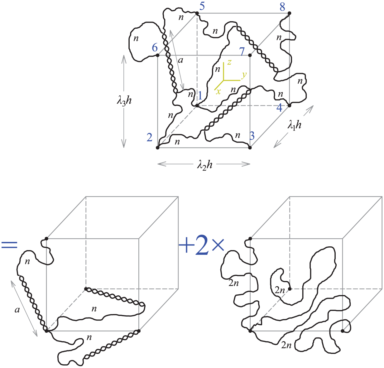
Under the Gaussian approximation, the topology of 3 four-node coil-rod structures in the faces of the rectangular prism is equivalent to combination of three three-chain networks.
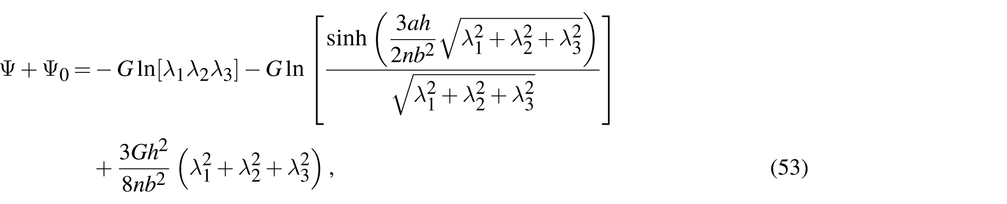
Similar to (4), the entropy of the deformed cell per unit reference volume can be written as
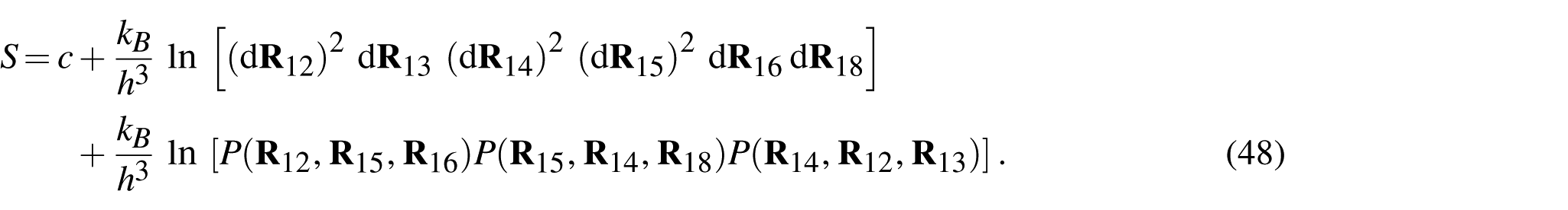
By defining
where

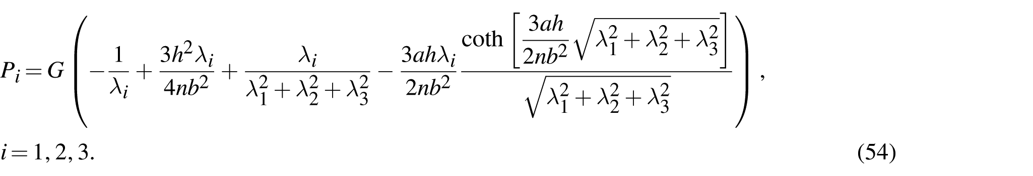
Analogous to the treatment in Section 3.1, the stress-free state at

By decomposing the four-node coil-rod structure positioned at each prism face into one two-node coil-rod and two coil structures, one can conclude that the three-dimensional network model is equivalent to the summation of three three-chain networks (Figure 7): one containing three two-node coil-rod structures on the prism edges, each having rod length a and n Kuhn segments in the coil; and two identical networks each containing three Gaussian coils with
In the literature, there is a correspondence between three-chain network models and a well-known type of material referred to as Valanis-Landel [22], where the strain energy is written as the sum of three scalar functions, each evaluated independently for three principal stretches. Due to the simplicity of this model, there are some generalizations for such network models, as shown by Ehret and Stracuzzi [23]. However, more involved network models, such as the eight-chain model, demonstrate superior performance in handling different types of experiments [7]. The comparison and relationship between the three-chain model and the eight-chain model are provided by Carroll [24] for pure coils without the presence of a junction zone. To examine the performance of the proposed network model (Figure 7), we formulate the eight-chain network model of the two-node coil-rod structure based on Moosavian and Tang [14], but with Gaussian approximation applied to the coil. Following the original model of Arruda and Boyce [7], eight two-node coil-rod structures are placed inside a diagonals of the cell with edges

where
where
Setting

Using the above relation, the initial stress-free state of the network with cube edge length h can be determined for given values of a and n.
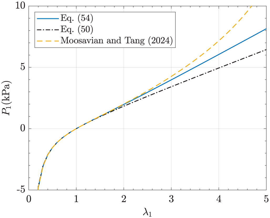
Figure 8 illustrates the difference between
4. Discussion
This study aimed to provide explicit modeling of interactions within junction zones, and it can be concluded that under the Gaussian statistics assumption, the two-node coil-rod structure network can be effectively applied. Based on the current framework, it is also possible to construct other three-dimensional network models, such as the symmetric eight-node structure with a rod, as elaborated in Appendix 3. However, a more detailed comparison between different networks requires testing them on real disordered biopolymer gels, where various mechanical tests are conducted on the samples.
It should be recalled that the phantom network model assumes that components can easily pass through each other. Therefore, the interaction between coils and rods can be extended by considering long-range interaction effects, such as excluded volume effects or entanglement between components [25–27], which would render the governing formulation more realistic but also computationally more challenging. In addition, the current work is based on the presence of a single rod within the unit cell. For a more comprehensive generalization, the inclusion of multiple rods and their associated configurations can be considered.
The unzipping behavior in disordered biopolymer gels is another intriguing topic that warrants future investigation. In this phenomenon, the rod can exchange segments with coils, resulting in a new configuration with longer coils and shorter rods. The conversion of the four-node coil-rod structure to a two-node coil-rod structure and two coils allows for the direct application of the previously developed unzipping formulation to the current framework [14]. Moreover, the Gaussian approximation for the coils is a more reasonable assumption in the presence of unzipping, as unzipping allows the system to adopt a new configuration to avoid high extension or entering the non-Gaussian regime. Finally, the current framework can incorporate different unzipping along different principal directions—an anisotropic feature that likely exists in reality but absent in the model developed by Moosavian and Tang [15].
5. Conclusion
This work provides preliminary insight into modeling junction zones and their explicit interactions with the amorphous regions in disordered biopolymer gels. The previous model of a two-node coil-rod structure is generalized to a four-node coil-rod structure, where two chains intertwine to form a common rod as a junction zone. The probability distribution function in the context of a phantom network is developed, which is mathematically more involved than the two-node coil-rod structure. Nevertheless, within the Gaussian statistics of the coils, the analytical probability distribution function can be derived with the aid of Fourier transform. It is demonstrated that, under this assumption, the four-node coil-rod structure is equivalent to a collection of two coils and one two-node coil-rod structure situated inside an affine network. This argument can also be generalized to multiple Gaussian coils sharing a single rod. To examine the characteristics of this structure, the four nodes are placed on the same plane to form a rectangular cell. The stress–stretch relationship of this network is derived, and the applicability of the Gaussian distribution is evaluated through comparison with the exact distribution. Finally, a three-dimensional network model is developed by arranging the four-node coil-rod structures on the faces of a rectangular prism. Results from this model is compared with the eight-chain network model combined with two-node coil-rod structure developed by Moosavian and Tang [14], which confirms that the network model with the two-node coil-rod structure is suitable for investigating the effects of more explicit interactions between coils and rods, as long as the Gaussian approximation for the coils remains valid. The proposed model provides a systematic framework for developing more complex networks that involve collections of coils connected by multiple rods.
Footnotes
Appendix 1
Appendix 2
Appendix 3
Declaration of conflicting interests
The authors declared no potential conflicts of interest with respect to the research, authorship, and/or publication of this article.
Funding
The authors disclosed receipt of the following financial support for the research, authorship, and/or publication of this article: TT acknowledges financial support from the Natural Sciences and Engineering Research Council of Canada (NSERC; Grant numbers: RGPIN-2018-04281, RGPAS-2018-522655) and Canada Research Chairs Program (Grant number: TIER1 2021-00023). HM acknowledges scholarship support from Alberta Innovates.