Comparison of the effects of a graded interphase and a homogeneous interphase on the macroscopic properties of a particulate composite

Abstract

Two conceptual models are reviewed for interphase zones that surround spherical inclusions in a particulate composite: a thin-shell layer within which the local conductivity of the interphase is uniform, and a graded interphase within which the local conductivity varies with radius according to a power law. The analysis is carried out in the context of thermal conductivity, but the analysis applies to all transport properties that are governed by a linear relation that is analogous to Fourier’s law, such as electrical conductivity (Ohm’s law), fluid flow through a permeable medium (Darcy’s law), and solute diffusion (Fick’s law). The question is posed as to whether a graded interphase can be replaced by a homogeneous-shell interphase, by some rational a priori choice of the shell thickness, so that the homogeneous-shell model leads to the same macroscopic effective conductivity as does the graded interphase model. Examination of some specific cases, as well as analysis of the analytical solution for the homogeneous interphase model, reveals that, in general, no single a priori choice of the shell thickness can yield an exact equivalence between the effects of the graded interphase and the homogeneous interphase, for all possible parameter ranges. However, for interphases in which the variation of the local conductivity is not too extreme, an expression is derived for the shell thickness that leads to approximate agreement between the graded interphase and homogeneous-shell interphase models.

Introduction

In many types of inclusion-in-matrix particulate (or fiber) composite materials, the inclusions are surrounded by a thin region in which the local physical properties (elastic moduli, thermal conductivity, etc.) are different from those of the pure matrix phase. One example is polymer fiber composites, in which a binding agent is sometimes applied to the fibers, to promote adhesion between the fiber and the matrix [1–3]. The binding agent diffuses into the matrix during the curing process, leading to a so-called “interphase zone” within which the local physical properties will vary with radius. Another example of a material containing an interphase zone is concrete, in which the porosity in the cement paste increases in the vicinity of the aggregate or sand inclusions, leading to a local radial variation of properties such as the elastic moduli and fluid permeability [4,5].

Two main types of models have been used to assess the effect of these interphase zones on the effective macroscopic properties. One approach is to assume that the interphase is a clearly delineated shell-like region surrounding the inclusion, within which the properties are locally uniform, but differ from those of the matrix [6,7]. Another type of model assumes that the local properties vary smoothly with radius. A convenient and versatile type of mathematical function for this variation is a power law [8,9].

The graded-interphase model is in many cases more physically realistic, but the homogeneous shell model permits a simpler mathematical analysis. In fact, the graded-interphase model has been shown to successfully account for the effect that the interphase zone in concrete (referred to in the concrete community as the interfacial transition zone) has on the elastic moduli [5] and on chloride ion diffusivity [10]. Although these two models have been used by many researchers to estimate the effect of the interphase on macroscopic properties, comparisons of the implications of the homogeneous-shell and graded-interphase models have been rare. Specifically, it would be interesting to know if a graded interphase can be replaced by some “equivalent” homogeneous-shell interphase. In the present paper, this issue will be investigated within the context of the effective conductivity problem for composites containing spherical inclusions.

The mathematical problem of calculating the effective conductivity is relevant to several transport-type processes that are governed by mathematically analogous sets of constitutive and balance equations, such as thermal conductivity, electrical conductivity, solute diffusivity, and the hydraulic permeability of a porous medium. Since heat conduction lends itself to a simple physical interpretation and very simple verbal discussion, the present problem will be presented within the context of thermal conductivity. But it should also be noted that, as proven by Lutz and Zimmerman [11], effective conductivity problems involving spherical inclusions are mathematically analogous to bulk modulus problems, for the special case in which all of the phases (matrix, inclusion, interphase) have zero Poisson ratio.

Single inclusion surrounded by a radially inhomogeneous interphase zone

Consider a spherical inclusion of radius a, in an infinite body that is subjected in the far-field to a uniform temperature gradient of magnitude G, aligned with the z–axis. If the thermal conductivity is a function of r, the steady-state temperature field is governed by the following equation [10,12]:

$$\frac{1}{r^2}\frac{\partial }{\partial r}\lfloor r^{2}k(r)\frac{\partial T}{\partial r}\rfloor +\frac{1}{r\sin \theta }\frac{\partial }{\partial \theta }\lfloor \sin \theta \frac{k(r)}{r}\frac{\partial T}{\partial \theta }\rfloor +\frac{1}{r\sin \theta }\frac{\partial }{\partial \varphi }\lfloor \frac{1}{\sin \theta }\frac{k(r)}{r}\frac{\partial T}{\partial \varphi }\rfloor =0,$$

(1)

where $(r,\theta ,\varphi )$ are the usual spherical coordinates. The far-field boundary conditions is

$$T=T_o+\mathrm{Gz}=T_o+\mathrm{Gr}\cos \theta ,\mathrm{as}r\to \mathrm{\infty },$$

(2)

where θ is the angle of rotation from the z-axis. Since the far-field temperature varies as $\cos \theta$ , and reduces to $T=T_o$ if the far-field gradient vanishes, the full temperature field will be of the form $T(r,\theta ,\varphi )=T_o+f(r)\cos \theta$ , where $f(r)\to \mathrm{Gr}$ as $r\to \mathrm{\infty }$ . Inserting this expression for $T(r,\theta ,\varphi )$ into equation (1) yields an ordinary differential equation for $f(r)$ :

$$k(r)[\frac{d^{2}f}{d{r}^2}+\frac{2}{r}\frac{\mathrm{df}}{\mathrm{dr}}-\frac{2}{r^2}f]+k\prime (r)\frac{\mathrm{df}}{\mathrm{dr}}=0.$$

(3)

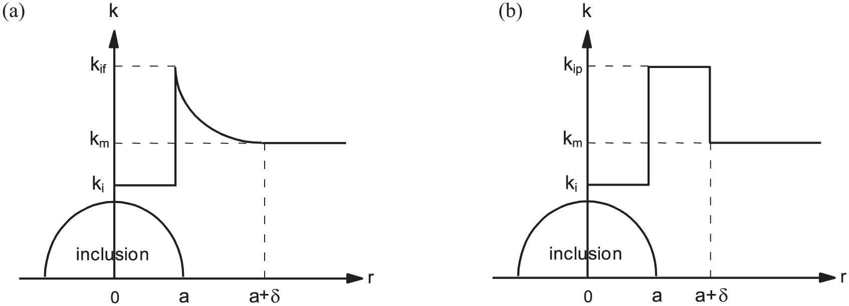
Several functional forms of the variation of local conductivity with radius have been investigated, such as linear, quadratic, exponential, and power law [13]. Following numerous authors [10,14–16], the conductivity in the interphase region surrounding the inclusion will be taken here to have a power-law variation as a function of radius (Figure 1(a)):

$$k(r)=k_m+(k_{\mathrm{if}}-k_m)(r/a{)}^{-\beta },$$

(4)

where subscript m denotes the “pure” matrix, and subscript if denotes the interface with the inclusion. The exponent β controls the “thickness” of the interphase zone. If the nominal thickness δ of the interphase zone is defined such that the conductivity perturbation $k(r)-k_m$ is 10% as large at $r=a+\delta$ as it is at $r=a$ , it would follow that $\beta \approx 2.3a/\delta$ [5]. If the nominal thickness of the interphase zone is defined by a 1% conductivity perturbation, then $\beta \approx 4.6a/\delta$ .

Figure 1.

(a) Inclusion of radius a, surrounded by an interphase zone in which the conductivity varies smoothly with radius. The nominal “thickness” of this interphase zone is δ. (b) Inclusion surrounded by a homogeneous-shell interphase zone, having a clearly defined thickness, δ.

Substitution of the conductivity variation given by equation (4) into equation (3) yields the following ordinary differential equation in the region $r>a$ outside of the inclusion:

$$[k_m+(k_{\mathrm{if}}-k_m)a^{\beta }{r}^{-\beta }][\frac{d^{2}f}{d{r}^2}+\frac{2}{r}\frac{\mathrm{df}}{\mathrm{dr}}-\frac{2}{r^2}f]-\beta a^{\beta }(k_{\mathrm{if}}-k_m)r^{-(\beta +1)}\frac{\mathrm{df}}{\mathrm{dr}}=0.$$

(5)

Theocaris [17] estimated values of β on the order of 100 for the interphase zone in a set of E-glass fiber / epoxy resin composites. Lutz et al. [5] found that values of β on the order of 20 were needed to fit the porosity gradient (and hence the property gradient) in the interfacial transition zone of concrete, based on SEM data from Crumbie [4]. On the other hand, nano-composites may often have interphase zone thicknesses that are on the same order of magnitude as the inclusion size, as pointed out by Sevostianov and Kachanov [18,19]. Although the analytical solutions presented below are valid for arbitrary interphase thicknesses, the discussion will focus on “thin” interphase zones, for which β can safely be taken to be a “large” integer.

If β is a positive integer greater than 3, the general solution of ODE equation (5) is [10]

$$f(r)=A_{1}r\sum _{n=0}^{\mathrm{\infty }}{\mathrm{\Gamma }}_{n\beta }(a/r{)}^{n\beta }+A_{2}r\sum _{n=0}^{\mathrm{\infty }}{\mathrm{\Gamma }}_{n\beta +3}(a/r{)}^{n\beta +3},$$

(6)

where $A_1$ and $A_2$ are arbitrary constants, ${\mathrm{\Gamma }}_0={\mathrm{\Gamma }}_3=1$ , and the subsequent non-zero ${\mathrm{\Gamma }}_n$ are obtained from the following recursion relationship:

$${\mathrm{\Gamma }}_{n+\beta }=-\left(\frac{k_{\mathrm{if}}-k_m}{k_m}\right)\frac{[n^2+(\beta -3)n-\beta ]}{(n+\beta )(n+\beta -3)}{\mathrm{\Gamma }}_n.$$

(7)

Sburlati and Cianci [15] have shown that, for the more general case in which β is not necessarily an integer, ODEs such as equation (5) can be solved in terms of hypergeometric functions. That approach, however, will not be pursued in the present paper.

The ratio test shows that the two series in equation (6) will both converge for all $r>a$ if $0<k_{\mathrm{if}}<2k_m$ , i.e., if the conductivity at the interface is either less than that of the pure matrix, or is no more than twice that of the pure matrix. For cases in which $k_{\mathrm{if}}>2k_m$ , the divergent series can be summed by applying an Euler transformation [20,21]. Another approach that could be taken when $k_{\mathrm{if}}>2k_m$ would be to reformulate the problem in terms of resistivity instead of conductivity, which leads to a convergent series for the function $f(r)$ when $k_{\mathrm{if}}>2k_m$ [10].

Inside the inclusion, which is assumed to be homogeneous with conductivity $k_i$ , the general solution to equation (3) is

$$f(r)=B_{1}r+B_2{r}^{-2}.$$

(8)

Boundedness of the temperature at the center of the inclusion requires that $B_2=0$ . The boundary condition at infinity, $f(r)\to \mathrm{Gr}$ , implies that $A_1=G$ . Continuity of the temperature at $r=a$ , as given by equation (6) outside the inclusion, and equation (8) inside the inclusion, leads to the condition

$$G\sum _{n=0}^{\mathrm{\infty }}{\mathrm{\Gamma }}_{n\beta }+A_2\sum _{n=0}^{\mathrm{\infty }}{\mathrm{\Gamma }}_{n\beta +3}=B_1.$$

(9)

Continuity of the radial component of the heat flux at $r=a$ implies continuity of $k(r)f\prime (r)$ , and leads to the condition

$$k_{\mathrm{if}}G\sum _{n=0}^{\mathrm{\infty }}{\mathrm{\Gamma }}_{n\beta }(1-n\beta )-k_{\mathrm{if}}{A}_2\sum _{n=0}^{\mathrm{\infty }}{\mathrm{\Gamma }}_{n\beta +3}(2+n\beta )=k_i{B}_1.$$

(10)

Equations (9) and (10) can be solved to yield

$$A_2=-G\lfloor \frac{(k_i-k_{\mathrm{if}})\sum _{n=0}^{\mathrm{\infty }}{\mathrm{\Gamma }}_{n\beta }+k_{\mathrm{if}}\sum _{n=0}^{\mathrm{\infty }}n\beta {\mathrm{\Gamma }}_{n\beta }}{(k_i-k_{\mathrm{if}})\sum _{n=0}^{\mathrm{\infty }}{\mathrm{\Gamma }}_{n\beta +3}+k_{\mathrm{if}}\sum _{n=0}^{\mathrm{\infty }}(n\beta +3){\mathrm{\Gamma }}_{n\beta +3}}\rfloor ,$$

(11)

with $B_1$ then given by equation (9).

Effective conductivity of a material containing inclusions surrounded by a power-law interphase zone

Many schemes have been devised to compute the effective conductivity of a particulate composite material, based solely on the solution to the single-inclusion problem. These approaches have been reviewed by, among others, Markov [22], Torquato [23], and Kachanov and Sevostianov [24]. One classical and simple method, which is known to be reasonably accurate, is the one originally proposed by Maxwell in the context of electrical conductivity [25–29]. Maxwell’s method leads to an effective conductivity of the form $k_{\mathrm{eff}}/k_m=(1+2\alpha c)/(1-\alpha c)$ , where c is the volume fraction of the inclusions, and α is a coefficient that depends on the inclusion geometry and the conductivities of the various phases. For small inclusion concentrations, the Maxwell prediction reduces to the dilute-concentration result, $k_{\mathrm{eff}}/k_m=1+3\alpha c$ . In the present paper, the comparison between the effect of a graded interphase, and the effect of a homogeneous thin-shell interphase, will be made based on comparison of the α factors. Hence, although the Maxwell formalism provides an elegant way to treat all microgeometries on equal footing, the main conclusions of this paper will not depend on accepting or assuming the accuracy of Maxwell’s homogenization method for large inclusion concentrations.

Maxwell’s approach considers a spherical region of radius R, containing N randomly located identical inclusions, where in the present case each inclusion is surrounded by its own interphase zone. Each inclusion causes a temperature perturbation in the far field, whose leading term is of order $r^{-2}$ . The total far-field perturbation due to all N inclusions is then assumed to simply be the sum of the perturbations due to each individual inclusion. This entire spherical region of radius R is then replaced with a homogeneous spherical region of radius R, having conductivity $k_{\mathrm{eff}}$ , and the temperature perturbation due to this hypothetical inclusion is calculated. Equating the leading far-field term of the temperature perturbation due to the “equivalent inclusion,” to the leading far-field term of the perturbation due to the collection of individual inclusions, then provides an implicit equation for $k_{\mathrm{eff}}$ .

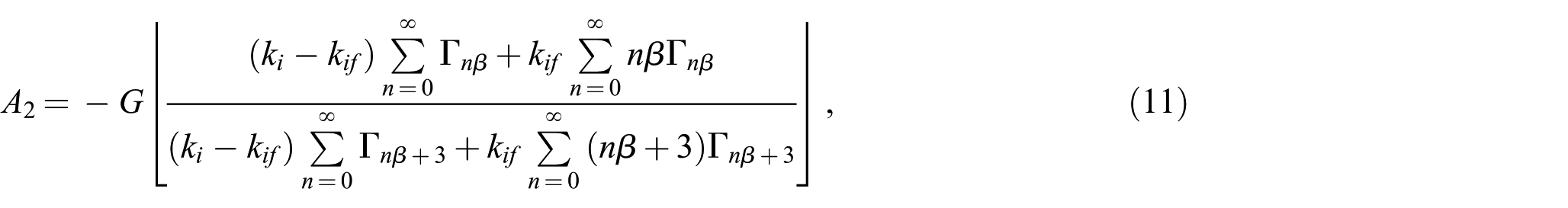
Each of the temperature perturbation terms varies as $\cos \theta$ , and so Maxwell’s method can be implemented by working with the function $f(r)$ . The two leading terms in the far-field behavior of $f(r)$ for a single inclusion are $f(r)=\mathrm{Gr}+A_2{a}^3{r}^{-2}$ , with $A_2$ given by equation (11). Since the term Gr corresponds to the temperature field that would exist in the absence of any inclusions, the perturbation due to the inclusion is $A_2{a}^3{r}^{-2}$ . If there are N inclusions within the spherical region of radius R, the total perturbation in $f(r)$ is $A_{2}N{a}^3{r}^{-2}$ . The perturbation caused by a single inclusion of radius R, having conductivity $k_{\mathrm{eff}}$ , is $G{R}^3{r}^{-2}(k_m-k_{\mathrm{eff}})/(2k_m+k_{\mathrm{eff}})$ [22]. Equating these two expressions, and noting that $N{a}^3{R}^{-3}$ is the volume fraction of inclusions, leads to [10]

$$\frac{k_{\mathrm{eff}}}{k_m}=\frac{1-(2A_2/G)c}{1+(A_2/G)c}.$$

(12)

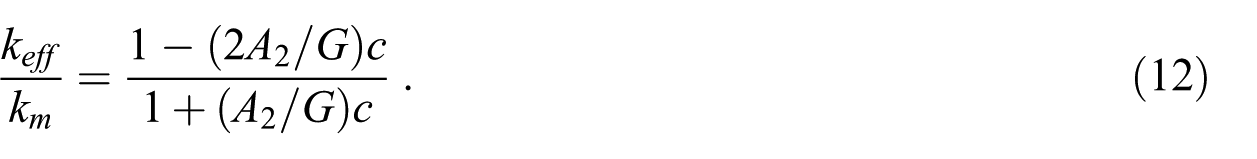
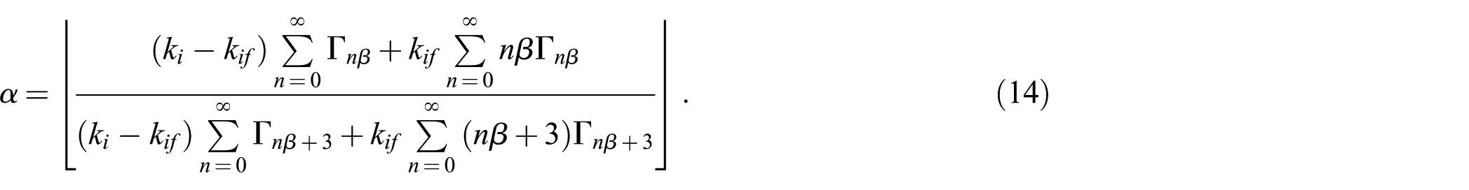
This result can be written in a simpler form by putting $-A_2/G=\alpha$ , which yields

$$\frac{k_{\mathrm{eff}}}{k_m}=\frac{1+2\alpha c}{1-\alpha c},$$

(13)

$$\alpha =\lfloor \frac{(k_i-k_{\mathrm{if}})\sum _{n=0}^{\mathrm{\infty }}{\mathrm{\Gamma }}_{n\beta }+k_{\mathrm{if}}\sum _{n=0}^{\mathrm{\infty }}n\beta {\mathrm{\Gamma }}_{n\beta }}{(k_i-k_{\mathrm{if}})\sum _{n=0}^{\mathrm{\infty }}{\mathrm{\Gamma }}_{n\beta +3}+k_{\mathrm{if}}\sum _{n=0}^{\mathrm{\infty }}(n\beta +3){\mathrm{\Gamma }}_{n\beta +3}}\rfloor .$$

(14)

The case of no interphase zone can be recovered by setting $k_{\mathrm{if}}=k_m$ in equation (14). Equations (7) and (14) then show that $\alpha =(k_i-k_m)/(k_i+2k_m)$ , from which it follows that equation (13) reduces to Maxwell’s famous result,

$$\frac{k_{\mathrm{eff}}}{k_m}=\frac{1+2[(k_i-k_m)/(k_i+2k_m)]c}{1-[(k_i-k_m)/(k_i+2k_m)]c}.$$

(15)

Single inclusion surrounded by a homogeneous thin-shell interphase zone

Another approach to modeling a particulate composite that contains inclusions that are surrounded by interphase zones is to assume that the interphase is a thin shell within which the conductivity is uniform (Figure 1(b)). Although this model has been discussed frequently in the literature [30–33], explicit expressions for the temperature profiles in the three regions (inclusion, interphase, matrix) do not seem to be readily available. Consider the geometry shown in Figure 1(b), in which the inclusion in the region $r<a$ has conductivity $k_i$ , the material in the interphase region $a<r<b$ has conductivity $k_{\mathrm{ip}}$ , and the matrix in the region $r>b$ has conductivity $k_m$ . In each of these three regions, the general solution for the function $f(r)$ will have the form given by equation (8). The constants in the inclusion will be denoted by $\{B_1,B_2\}$ , the constants in the interphase will be denoted by $\{C_1,C_2\}$ , and the constants in the matrix will be denoted by $\{A_1,A_2\}$ . Boundedness of the temperature at the center of the inclusion requires that $B_2=0$ , and the boundary condition at infinity implies that $A_1=G$ .

The other four constants are found by imposing continuity of the temperature and the radial component of the heat flux at $r=a$ and $r=b$ . These four conditions take the following forms:

$$\mathrm{Continuity}\mathrm{of}\mathrm{temperature}\mathrm{at}r=a:B_{1}a=C_{1}a+C_2{a}^{-2},$$

(16)

$$\mathrm{Continuity}\mathrm{of}\mathrm{temperature}\mathrm{at}r=b:C_{1}b+C_2{b}^{-2}=\mathrm{Gb}+A_2{b}^{-2},$$

(17)

$$\mathrm{Continuity}\mathrm{of}\mathrm{heat}\mathrm{flux}\mathrm{at}r=a:k_i{B}_1=k_{\mathrm{ip}}{C}_1-2k_{\mathrm{ip}}{C}_2{a}^{-3},$$

(18)

$$\mathrm{Continuity}\mathrm{of}\mathrm{heat}\mathrm{flux}\mathrm{at}r=b:k_{\mathrm{ip}}{C}_1-2k_{\mathrm{ip}}{C}_2{b}^{-3}=k_{m}G-2k_m{A}_2{b}^{-3}.$$

(19)

The values of these four constants can be found by solving equations (16)–(19). The full set of six constants can then be summarized as follows:

$$A_1=G,$$

(20)

$$A_2=\frac{(k_m-k_{\mathrm{ip}})(k_i+2k_{\mathrm{ip}})b^3+(k_{\mathrm{ip}}-k_i)(k_m+2k_{\mathrm{ip}})a^3}{(k_{\mathrm{ip}}+2k_m)(k_i+2k_{\mathrm{ip}})+2(k_{\mathrm{ip}}-k_i)(k_m-k_{\mathrm{ip}}){(a/b)}^3}G,$$

(21)

$$B_1=\frac{9k_m{k}_{\mathrm{ip}}G}{(k_{\mathrm{ip}}+2k_m)(k_i+2k_{\mathrm{ip}})+2(k_{\mathrm{ip}}-k_i)(k_m-k_{\mathrm{ip}}){(a/b)}^3},$$

(22)

$$B_2=0,$$

(23)

$$C_1=\frac{3k_m(k_i+2k_{\mathrm{ip}})G}{(k_{\mathrm{ip}}+2k_m)(k_i+2k_{\mathrm{ip}})+2(k_{\mathrm{ip}}-k_i)(k_m-k_{\mathrm{ip}}){(a/b)}^3},$$

(24)

$$C_2=\frac{3k_m(k_{\mathrm{ip}}-k_i)G{a}^3}{(k_{\mathrm{ip}}+2k_m)(k_i+2k_{\mathrm{ip}})+2(k_{\mathrm{ip}}-k_i)(k_m-k_{\mathrm{ip}}){(a/b)}^3}.$$

(25)

Effective conductivity of a material containing inclusions surrounded by a homogeneous thin-shell interphase zone

The effective conductivity for this microstructure can again be estimated using Maxwell’s formalism. The far-field perturbation of $f(r)$ for a single inclusion surrounded by a homogeneous thin-shell interphase zone is $A_2{r}^{-2}$ , with $A_2$ now given by equation (21). This expression differs slightly from the analogous expression for the case of a graded interphase, since the leading term in the second series in equation (6) contains a term $a^3$ , whereas in the present problem, the term $a^3$ has been implicitly absorbed into $A_2$ . If there are N inclusions contained within the spherical region of radius R, the total perturbation in $f(r)$ is $A_{2}N{r}^{-2}$ . The perturbation in $f(r)$ outside of the “equivalent” inclusion of radius R is again given by $G{R}^3{r}^{-2}(k_m-k_{\mathrm{eff}})/(2k_m+k_{\mathrm{eff}})$ . Equating these two expressions, and noting that $N{a}^3{R}^{-3}$ is the volume fraction of inclusions, leads to

$$\frac{k_{\mathrm{eff}}}{k_m}=\frac{1-(2A_2/G{a}^3)c}{1+(A_2/G{a}^3)c}.$$

(26)

This result can be written in the same form as equation (13) by defining $\alpha =-A_2/G{a}^3$ , thereby yielding

$$\alpha =-\frac{(k_{\mathrm{ip}}-k_i)(k_m+2k_{\mathrm{ip}})+(k_m-k_{\mathrm{ip}})(k_i+2k_{\mathrm{ip}}){(b/a)}^3}{(k_{\mathrm{ip}}+2k_m)(k_i+2k_{\mathrm{ip}})+2(k_m-k_{\mathrm{ip}})(k_{\mathrm{ip}}-k_i){(a/b)}^3}.$$

(27)

The correctness of the above results can be checked by examining various special cases. If $k_{\mathrm{ip}}=k_m$ , then equation (21) yields $A_2=-G{a}^3(k_i-k_m)/(k_i+2k_m)$ , and equation (27) yields $\alpha =(k_i-k_m)/(k_i+2k_m)$ , which is Maxwell’s result for the case of spherical inclusions without an interphase zone. If $k_{\mathrm{ip}}=k_i$ , then equation (21) yields $A_2=-G{b}^3(k_i-k_m)/(k_i+2k_m)$ , which is the same result as the previous case, except that the inclusions now have radius b instead of a. If $k_{\mathrm{ip}}=0$ , then the inclusion + interphase should act like a non-conducting inclusion of radius b, regardless of the value of $k_i$ . In this case, equation (21) shows that $A_2=0.5G{b}^3$ , which is indeed the classical Maxwell result for a non-conducting inclusion of radius b. If $k_{\mathrm{ip}}\to \mathrm{\infty }$ , then the inclusion + interphase should act like a super-conducting inclusion of radius b. In this case, equation (21) shows that $A_2=-G{b}^3$ , which is Maxwell’s result for a super-conducting inclusion of radius b. Finally, if $b=a$ , equation (27) again reduces to $\alpha =(k_i-k_m)/(k_i+2k_m)$ , Maxwell’s result for spherical inclusions without an interphase zone.

The complexity of expression (27) does not permit a simple understanding of the relative influences of the interphase conductivity $k_{\mathrm{ip}}$ and the interphase thickness $\delta =b-a$ . Some insight can be gained by focusing on the two cases of non-conducting and super-conducting inclusions. These two cases are not only end-members in some sense, but also have the advantage of permitting the effect of the interphase to be isolated from the effect of the inclusion. For non-conducting inclusions, $k_i=0$ , and thin interphase zones, i.e., $\delta =b-a<<a$ , equation (27) reduces, after some algebraic manipulation, to

$$\alpha =-\frac{1}{2}[1-3\frac{(k_{\mathrm{ip}}-k_m)}{k_m}\left(\frac{\delta }{a}\right)].$$

(28)

to first order in $\delta /a$ . Recalling that $\alpha =-0.5$ is the result for “non-conducting inclusions, no interphase,” it is seen that the relative conductivity increment in the interphase, $(k_{\mathrm{ip}}-k_m)/k_m$ , multiplied by the normalized interphase thickness $\delta /a$ , controls the influence of the interphase zone on the effective conductivity. The factor of 3 is a geometric factor that arises from the approximation $(b/a{)}^3=[1+(\delta /a{)]}^3\approx 1+3(\delta /a)$ .

In the other end-case of super-conducting inclusions, equation (27) reduces to

$$\alpha =1+3\left(\frac{k_{\mathrm{ip}}-k_m}{k_{\mathrm{ip}}}\right)\left(\frac{\delta }{a}\right)=1-3\left(\frac{{\rho }_{\mathrm{ip}}-{\rho }_m}{{\rho }_m}\right)\left(\frac{\delta }{a}\right),$$

(29)

where $\rho =1/k$ is the resistivity. (Note that whereas equation (27) applies for interphases having arbitrary thicknesses, equation (28) and equation (29) are valid only to first order in the normalized interphase thickness, $\delta /a$ ). Since $\alpha =1$ is the result for “super-conducting inclusions, no interphase,” in this case the effect of the interphase is controlled by the product of the relative resistivity increment multiplied by the normalized interphase thickness. The relative resistivity increment and relative conductivity increment will be numerically close for very weakly inhomogeneous interphases, but will differ substantially if either increment exceeds about 20%. Consequently, the example discussed above casts some doubt on whether a single inhomogeneity parameter can be found that controls the value of α, over the entire possible parameter space.

Homogeneous interphase that is “equivalent” to a graded interphase

An interesting question to ask, for the purposes of estimating the overall effective conductivity, is whether a power-law graded interphase can be replaced by some “equivalent” homogeneous thin-shell interphase [18]. Some thought soon reveals that, if both the interphase conductivity $k_{\mathrm{ip}}$ and the interphase thickness $b-a$ are allowed to be free parameters, there will always be many pairs of values of these parameters that cause equation (26) to agree with equation (13) for any given graded interphase. A comparison between the graded interphase and the uniform interphase could be made on the basis of assuming that the interphase thickness for the thin-shell model is identified with the region (in the graded-interphase model) in which the conductivity perturbation is greater than, say, 10% of its maximum value. However, this cut-off of a 10% conductivity variation is somewhat arbitrary, and quite different results would be obtained if this cut-off were set to 1%, for example [34]. A non-arbitrary basis on which to make the comparison is to ask the following question: if the conductivity $k_{\mathrm{ip}}$ in the thin-shell model is taken to equal the interface conductivity $k_{\mathrm{if}}$ in the graded-interphase model, what value should be chosen for the interphase thickness $b-a$ so as to cause the two interphases to have the same effect on the macroscopic effective conductivity?

This topic was investigated by Wang and Jasiuk [9], for the elastic moduli of a particulate composite. (Recall again that Lutz and Zimmerman [11] proved an exact mathematical correspondence between the effective conductivity and the effective bulk modulus, for the special case of zero Poisson ratio). Wang and Jasiuk assumed a power-law interphase, with a clearly defined thickness, so that, with reference to geometries such as shown in Figure 1(a), the conductivity of the interphase at $r=b$ exactly matches the conductivity of the matrix. However, they also assumed that the conductivity of the interphase at $r=a$ exactly matches the conductivity of the inclusion. Hence, their conductivity profiles were always continuous, and monotonic, throughout the inclusion, interphase, and matrix. This is clearly a very special sub-case of materials with interphase zones, and could not, for example, represent properties such as the diffusivity of concrete, for which $k_i=0$ , but $k_{\mathrm{ip}}>0$ , or the bulk modulus of concrete, for which $K_{\mathrm{ip}}<<K_i$ . With these caveats in mind, it is worth noting that Wang and Jasiuk [9] concluded that making the “obvious” identification of $K_{\mathrm{ip}}$ with the volumetrically-weighted mean value of $K(r)$ within the actual graded interphase leads to close agreement between the effective moduli for the case of a graded interphase and the case of a homogeneous interphase, each having the same thickness.

Another set of investigations that are closely related to the topic of the present paper are those that were conducted by Sevostianov and Kachanov [19] regarding the elastic moduli, and by Sevostianov [14] for the thermal pressure coefficient (the product of the bulk modulus and the thermal expansion coefficient). These researchers looked at various property profiles in the interphase zone around a spherical inclusion, and endeavored to “replace” the inclusion + interphase with an “equivalent” inclusion. They considered linear and power-law property variations within the interphase, but did not consider the homogeneous thin-shell model. Some qualitative trends were observed, but it was noted that these trends were not obeyed for a power-law interphase in which, in the present notation, $K_{\mathrm{if}}=0.1K_m$ , i.e., for cases in which there is a relatively large variation of the bulk modulus within the interphase zone.

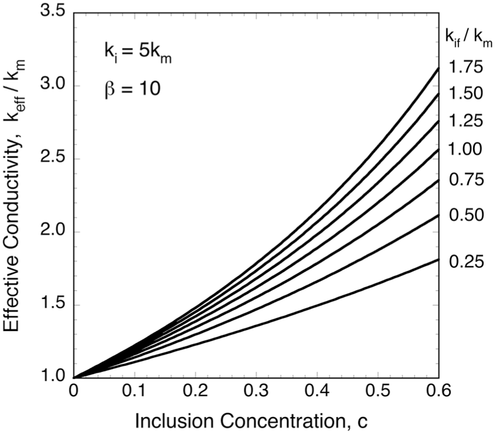
To investigate the question posed at the top of this section, consider a composite material containing spherical inclusions of radius a, having $k_i=5k_m$ . Each inclusion is surrounded by a power-law graded interphase, as described by equation (4), with $\beta =10$ , which corresponds to an interphase whose thickness is about 1/8th of the inclusion diameter. Figure 2 shows the normalized effective conductivity of this composite, as computed from equation (13), for a range of values of $k_{\mathrm{if}}/k_m$ . Table 1 also shows the α factor for each of these cases, as given by equation (14).

Figure 2.

Normalized effective conductivity of a material containing spherical inclusions that are five times more conductive than the pure matrix, each surrounded by a power-law interphase zone, with β = 10.

Table 1.

Data for spherical inclusions, with $k_i/k_m=5$ , and $\beta =10$ .

$\frac{k_{\mathrm{if}}-k_m}{k_m}$	$k_{\mathrm{if}}/k_m$	α equation (27)	$\delta /a$ estimated bymatching α	α estimated fromequations (30) and (31)	αestimated fromequations (32) and (33)
0.75	1.75	0.690	0.146	0.658	0.672
0.50	1.50	0.656	0.140	0.638	0.647
0.25	1.25	0.616	0.128	0.609	0.615
0.00	1.00	0.571	–	–	–
−0.25	0.75	0.518	0.104	0.514	0.507
−0.50	0.50	0.452	0.084	0.417	0.398
−0.75	0.25	0.355	0.046	0.205	0.167

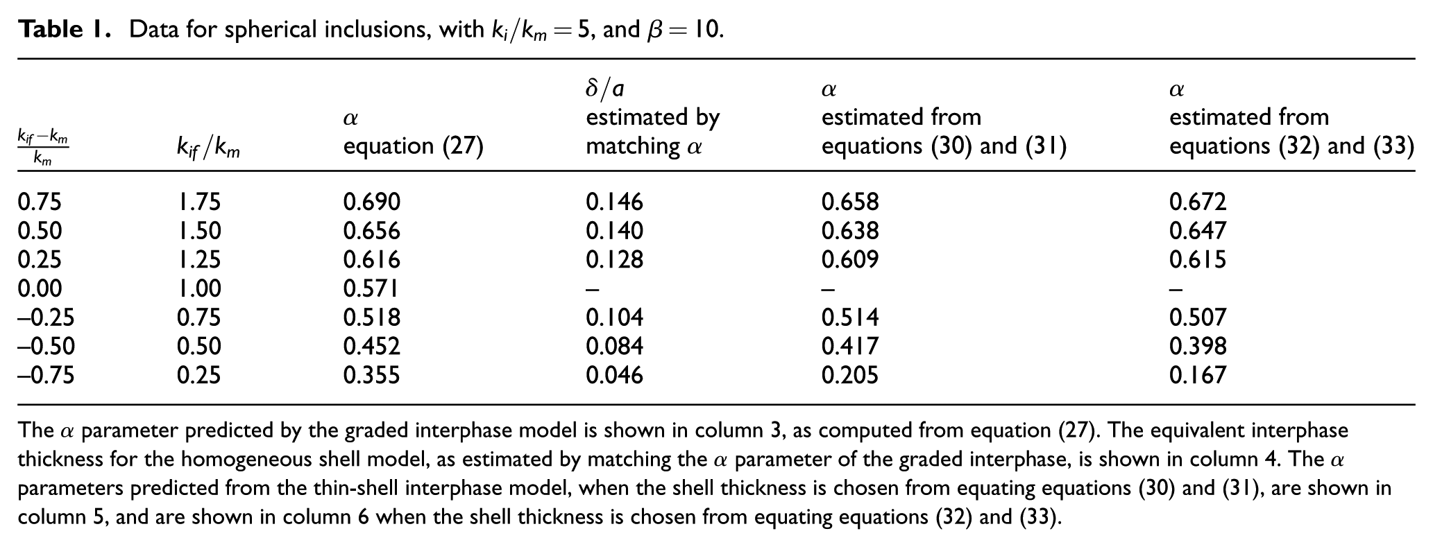
The α parameter predicted by the graded interphase model is shown in column 3, as computed from equation (27). The equivalent interphase thickness for the homogeneous shell model, as estimated by matching the α parameter of the graded interphase, is shown in column 4. The α parameters predicted from the thin-shell interphase model, when the shell thickness is chosen from equating equations (30) and (31), are shown in column 5, and are shown in column 6 when the shell thickness is chosen from equating equations (32) and (33).

If this interphase zone is modeled instead by a homogeneous shell of thickness δ, with $k_{\mathrm{ip}}$ chosen to equal $k_{\mathrm{if}}$ (cf. Figure 1), equation (27) can be inverted to yield the value of $(b/a)=1+(\delta /a)$ that will lead to the same α factor as does the graded interphase model. These values of $\delta /a$ are listed in column 4 of Table 1. As expected, these values are all somewhat smaller than the nominal “thickness” of the graded interphase, which is roughly given in this case by $\delta /a\approx 2.3/\beta =0.23$ . Very roughly, the effective thickness of the homogeneous interphase shell is about one-half of the nominal thickness of the graded interphase. However, even for this restricted family of cases, with a relatively moderate variation of conductivity within the interphase, the optimal homogeneous-shell thickness varies noticeably from case to case.

To proceed further, one can ask the following question: can the “effective thickness” of the hypothetical uniform interphase be related, in some rational manner, to the β parameter in the graded interphase model? One plausible way to do this might be to equate the “area under the curve” of the two $k(r)$ functions (again, see Figure 1). This could be done in two obvious ways, based either on a straightforward “linear” integration of $k(r)$ with respect to r, or a volumetric integral of $k(r)$ with respect to the volume increment, $4\pi r^2\mathrm{dr}$ [34]. A priori, it is not clear if either of these methods will yield accurate estimates of the effective interphase thickness. Wang and Jasiuk [9] found that both integration methods yielded similar results for the microstructures that they examined, which had spatial variation, but no discontinuities, in the local properties. The predictions of the two integration methods will of course coalesce for very thin interphases.

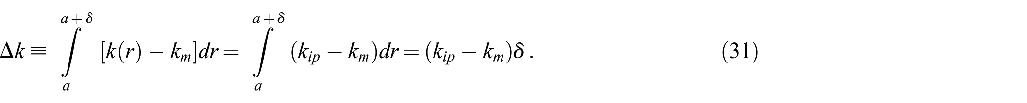
To avoid the fact that the integral of $k(r)$ from $r=a$ to $r=\mathrm{\infty }$ will diverge for the graded interphase, and guided by equation (28), it is convenient to work with the “excess conductivity”, $k(r)-k_m$ . According to equation (4), $k(r)-k_m=(k_{\mathrm{if}}-k_m)(r/a{)}^{-\beta }$ . Since it is necessarily the case that $\beta >1$ , the integral of the excess conductivity will always converge. Using the linear integration approach, the total excess conductivity of the graded interphase is given by

$$\mathrm{\Delta }k\equiv \underset{a}{\overset{\mathrm{\infty }}{\int }}[k(r)-k_m]\mathrm{dr}=(k_{\mathrm{if}}-k_m)\underset{a}{\overset{\mathrm{\infty }}{\int }}{(r/a)}^{-\beta }\mathrm{dr}=(k_{\mathrm{if}}-k_m)\frac{a}{\beta -1},$$

(30)

whereas the total excess conductivity of the homogeneous interphase is given by

$$\mathrm{\Delta }k\equiv \underset{a}{\overset{a+\delta }{\int }}[k(r)-k_m]\mathrm{dr}=\underset{a}{\overset{a+\delta }{\int }}(k_{\mathrm{ip}}-k_m)\mathrm{dr}=(k_{\mathrm{ip}}-k_m)\delta .$$

(31)

If the conductivity of the hypothetical homogeneous interphase, $k_{\mathrm{ip}}$ , is set equal to the interface conductivity of the graded interphase, $k_{\mathrm{if}}$ (see Figure 1), then equation (31) reduces to $\mathrm{\Delta }k=(k_{\mathrm{if}}-k_m)\delta$ . Equating the two expressions derived above for the excess conductivity then yields $\delta /a=1/(\beta -1)$ as an estimate of the effective interphase thickness. For the geometry considered I Table 1 and Figure 2, with $\beta =10$ , this model predicts $\delta /a=0.111$ .

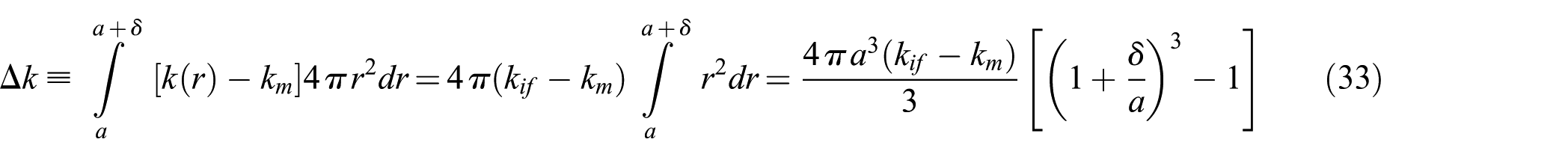
A similar calculation using the volumetric integration approach yields

$$\mathrm{\Delta }k\equiv \underset{a}{\overset{\mathrm{\infty }}{\int }}[k(r)-k_m]4\pi r^2\mathrm{dr}=4\pi (k_{\mathrm{if}}-k_m)\underset{a}{\overset{\mathrm{\infty }}{\int }}{(r/a)}^{-\beta }{r}^2\mathrm{dr}=\frac{4\pi a^3(k_{\mathrm{if}}-k_m)}{\beta -3}$$

(32)

for the graded interphase, and

$$\mathrm{\Delta }k\equiv \underset{a}{\overset{a+\delta }{\int }}[k(r)-k_m]4\pi r^2\mathrm{dr}=4\pi (k_{\mathrm{if}}-k_m)\underset{a}{\overset{a+\delta }{\int }}{r}^2\mathrm{dr}=\frac{4\pi a^3(k_{\mathrm{if}}-k_m)}{3}[{(1+\frac{\delta }{a})}^3-1]$$

(33)

for the homogeneous interphase. For thin interphases, i.e., $\delta /a<<1$ , the right side of equation (33) reduces to $4\pi a^3(k_{\mathrm{if}}-k_m)(\delta /a)$ , in which case equating expressions (32) and (33) yields $\delta /a=1/(\beta -3)$ . Since thin interphase zones correspond to large values of β, both the linear and the volumetric integration methods essentially lead to $\delta /a=1/\beta$ for very thin interphases. For the general case of an interphase zone of arbitrary thickness, equating expressions (32) and (33) leads to $\delta /a=[\beta /(\beta -3{)]}^{1/3}-1$ . For interphases with $\beta =10$ , this model predicts $\delta /a=0.126$ .

The two ways of estimating the effective interphase thickness yield reasonably close values in this example, with $\beta =10$ ; recall that the two methods coalesce for very thin interphases (very large values of β). These values are, as expected, roughly half of the nominal thickness of the graded interphase, as would be estimated based on the region over which the conductivity differs noticeably from that of the matrix.

However, the more pertinent question to ask is: if the interphase thickness is chosen using one of these two “area under the conductivity curve” approaches, will the value of α predicted by the thin-shell interphase model agree with that predicted by the graded interphase model? Columns 5 and 6 of Table 1 show that values of α predicted by these two approaches. For interphases that are only weakly inhomogeneous, both methods yield accurate values of α. This broadly agrees with the findings of Wang and Jasiuk [9], who only examined materials in which the local properties varied monotonically with radius. However, as can be seen in the bottom row of Table 1, the agreement deteriorates as the local conductivity variation within the interphase become more extreme, which is in qualitative agreement with the results of Sevostianov and Kachanov [19].

Summary and conclusions

Two conceptual models have been reviewed for interphase zones that surround spherical inclusions in a particulate composite. One model is that of a thin-shell layer within which the conductivity of the interphase is uniform. The other model assumes that the local conductivity outside of the inclusion varies radially, according to an $r^{-\beta }$ power law, asymptotically approaching the conductivity of the matrix phase as r increases. If Maxwell’s effective medium method is used to predict the effective conductivity, expressions are obtained having the form $k_{\mathrm{eff}}/k_m=(1+2\alpha c)/(1-\alpha c)$ , where c is the volume fraction of the inclusions, and α is a coefficient that depends on the inclusion and interphase geometry, and the conductivities of the various phases. For small inclusion concentrations, the Maxwell prediction reduces to the dilute-concentration result, $k_{\mathrm{eff}}/k_m=1+3\alpha c$ , which is “exact” for small value of c. Hence, the effect of different inclusions can be compared based on the α factors.

The question was then posed as to whether a graded interphase could be replaced by a homogeneous thin-shell interphase, by some rational, a priori, choice of the shell thickness. A specific case was examined of a material containing conductive inclusions $(k_i/k_m=5)$ , with a graded interphase zone that was either more or less conductive than the matrix. The nominal thickness of the graded interphase was about 1/8th of an inclusion diameter. Even for cases of only moderate variation of the conductivity within the interphase, it was found that no single choice of the shell thickness will yield a precise equivalence between the effect of the graded interphase and the homogeneous interphase. For interphases that are not “too inhomogeneous,” i.e., for $|k_{\mathrm{if}}-k_m|/k_m<0.5$ , an appropriate thin-shell thickness can be chosen by matching the areas under the “excess conductivity” curves, so that the thin-shell model yields effective conductivity values that agree closely with the graded interphase model. For interphases with more extreme conductivity variations, the two models will not closely agree.