A first-gradient approach to the remodeling and fluid flow in saturated porous media

Abstract

We rephrase Gurtin and Anand’s formulation of strain-gradient plasticity (“A theory of strain-gradient plasticity for isotropic, plastically irrotational materials. Part II: Finite deformations”. Int. J. Plasticity, 2005) to describe the isochoric structural transformations (remodeling) of multicellular aggregates in in silico compression tests. We consider solid–fluid biphasic media, thereby accounting for interactions that cannot arise in classical elasto-plastic materials. To gain insight into the behavior of the fluid, especially in the proximity of the aggregate’s boundary, we introduce a Darcy–Brinkman model, coupled with the deformation of the solid. This results in a constitutive framework of grade 1 in the fluid velocity (Darcy’s law is of grade 0), wherein the stress tensor of the fluid acquires a dissipative contribution. To obtain the equations determining the system’s evolution, we adopt the Principle of Virtual Power, which allows us to handle explicitly the internal constraints of incompressibility of the solid–fluid mixture and of isochoricity and null-spin of the remodeling rate tensor. Furthermore, we enforce the Principle of Maximum Dissipation to justify the generalized dissipative forces of our model. Finally, we discuss some relevant results of a numerical experiment, and we provide a brief computational background for the initial- and boundary-value problem representing our model.

1. Introduction

The mechanical behavior of soft and hydrated biological tissues is often studied by having recourse to the theory of mixtures [1–6]. Within a minimal modeling approach, a tissue of the aforementioned class may be described as a mixture comprehending a solid phase and a fluid phase [1,5,7,8]. The solid phase idealizes the complex of cells, extracellular matrix, protein links, and many other species. The fluid phase represents the tissue’s interstitial fluid, mostly consisting of water, macromolecules, nutrients, ions, and various chemical substances or compounds.

In this work, with the terminology “biological tissues,” we intend both true tissues (e.g., articular cartilage, muscles, blood vessels or skin) and cultures of cells. Such cultures are often referred to as multicellular aggregates and are important to study, through in vitro or in silico experiments, the mechanical behavior of tumor masses [9,10] before vascularization begins.

As is common for living matter, biological tissues experience changes of their material properties [11,12], which can be viewed as the result of the activation of some specific structural degrees of freedom. In general, such changes are dynamically coupled with transformations of morphology and shape, although being virtually independent of those. Given suitable time and length scales, the structural changes may be primarily related to genetics [12], physio-pathological events [13], aging [14], as well as to a variety of possibly concurring stimuli, which include mechanical, chemical, and electromagnetic interactions of the tissue with its surrounding environment.

The structural transformations experienced by a tissue are often conventionally classified on the basis of the phenomena by which they are predominantly characterized (see, e.g., Taber [12]): the uptake or loss of mass, and the structural rearrangements associated with these processes, constitute growth; the (usually mass-preserving) reorganization of the internal structure of a tissue is referred to as remodeling and pertains, for example, to the transformations of the extracellular matrix or to the breaking and reconstruction of the intercellular bonds [10,15]; the production of patterns, and the processes yielding the specific morphology and size of a tissue are the primary expressions of morphogenesis [16]. Other essential processes for the evolution of a tissue are cellular differentiation and migration.

Although the distinction among growth, remodeling, and morphogenesis is not sharp [12], it is possible to determine time scales and experimental settings in which each of these phenomena is preponderant with respect to the others. In the remainder of this work, we concentrate exclusively on remodeling, and we consider the specific case in which it occurs in multicellular aggregates undergoing compression tests [9,10].

The aforementioned tissutal transformations are often described by a second-order tensor field, termed remodeling tensor from here on, that is conceived with the property of being incompatible, i.e., not expressible as the Jacobian tensor field of a deformation (see, e.g., the seminal papers by Rodríguez et al. [17], Epstein and Maugin [18], and the works by Vandiver and Goriely [19], Yavari [20], Yavari and Goriely [21] and Goriely [22]). In fact, according to a somewhat standard praxis, the remodeling tensor is taken as one of the factors that decompose multiplicatively the deformation gradient tensor of a medium undergoing remodeling, which, instead, is by definition the Jacobian tensor field of the deformation. If such decomposition features two factors only, the first factor is usually identified with an accommodating tensor field, which is incompatible, too, and compensates for the incompatibility of the remodeling tensor. Often, the accommodating tensor is assumed to describe elastic distortions, whereas the remodeling tensor is attributed intrinsically inelastic nature and is thus said to describe anelastic distortions.

The studies on remodeling available in the literature which we are aware of are mainly developed upon theories of “grade zero” [23] in the remodeling tensor. Accordingly, the dependence of the remodeling tensor on the points of a medium is not resolved explicitly by accounting for its gradient, or higher-order derivatives, in the list of the basic variables with which the mathematical models are constructed and, in particular, the constitutive framework is established (see, e.g., [5,6,12,17,23–29]). However, theories of remodeling and growth of grade 1 or higher can also be found, and were proposed, e.g., by Epstein and Maugin [18], Epstein [30,31], Epstein and Elżanowski [32], Goriely [22] and, later, by Grillo et al. [33] and by Grillo and Di Stefano [34–36]. Still, to the best of our knowledge, they have not been given the attention that grade-0 theories have received.

Conversely, in plasticity, higher-order effects are well established and studied, since the inclusion of such effects is necessary for capturing size-related phenomena (see, e.g., the review of strain-gradient plasticity by Voyiadjis and Song [37]). Theories of plasticity that do not account for the gradients of their inelastic descriptors are unable to recover the stress–strain curves obtained, for example, in indentation, torsion, and bending tests for metals at low scales. In biomechanics, however, low-scale mechanical tests on biological tissues are rather common, and assessing the effectiveness of the grade-0 theories of remodeling may become an interesting topic, especially to evaluate when it is convenient to switch to theories of higher grade. Aside from that, the theories of higher order are interesting, at least, for other two reasons: they may unravel boundary effects due to the contact interactions between the tested tissues and the experimental apparatus, and they make it possible to blend the mere phenomenological aspects of remodeling with those pertaining to phase transitions and to the generation of patterns typical of morphogenesis [18]. These are, in fact, our main motivations for undertaking a strain-gradient formulation of remodeling, which we obtain by re-proposing the work by Gurtin and Anand [38] on plasticity in the biomechanical context of the compression tests of multicellular aggregates.

In conjunction with remodeling, another major role on the evolution of the aforementioned systems is played by the interactions between the interstitial fluid and the solid phase. The models of fluid mostly encountered in the literature assume Darcy’s law, which is often provided in the form of a linear relation between the velocity of the fluid relative to the solid and the pressure gradient of the fluid. The pressure gradient is multiplied from the left by the permeability tensor, which contains important pieces of information about the pore space and material symmetries of the porous medium under study, and is usually coupled with the deformation [1]. In our work, however, we abandon Darcy’s law in favor of an enriched description of the fluid known as Darcy–Brinkman model. Our motivation is twofold. First, in addition to the interactions resolved within the Darcian approach, the Darcy–Brinkman model accounts also for self-interactions of the fluid, resulting in a dissipative contribution to the overall stress tensor, usually taken linear in the fluid velocity gradient. Indeed, due to the presence of macromolecules, nutrients, and other substances dissolved in the fluid, the assumption of negligible viscosity may not hold, and the fluid flow may be non-Darcian. Second, at variance with Darcy’s law, the Darcy–Brinkman model allows for describing “boundary effects” [39,40]. We mention that, before us, other, pioneering, works employed an extension of Darcy’s law, named Brinkman equation [41], to study the interstitial flow in biological media [42,43].

This work is organized as follows: Section 2 presents the relevant modeling hypotheses for hydrated soft tissues, the kinematic framework (with all the considered constraints), and the mass balance laws; Section 3 summarizes all the force balances and the constraints, after formulating the Principle of Virtual Power [44,45] (PVP) for constrained systems, and for a grade-1 theory both in the remodeling tensor [38] and in the velocity field of the fluid phase (at variance with previous works of our group—see, e.g., Grillo and Di Stefano [34,35] and Giammarini et al. [46]—we provide some notions about the functional spaces involved in the formulation); Section 4 presents the constitutive framework; Section 5 shows the initial- and boundary-value problem to be solved and contains a discussion on some numerical results; Section 6 provides some concluding remarks.

2. Hydrated soft tissues as biphasic mixtures undergoing remodeling

We present the main hypotheses with which we describe the mechanics of fluid-saturated soft tissues undergoing remodeling of their internal structure. As “representative” for this kind of biological systems we refer to the so-called “multicellular aggregates” [10]. These are conglomerates of various types of cultured cells that are typically used in laboratory experiments on the mechanics of tumor spheroids [47]. The latter ones, in turn, inspire mechanical models of the evolution of in situ tumors in the stages of their growth that precede vascularization [48,49].

In the mechanics of multicellular aggregates, it is often assumed that remodeling is a volume-preserving process, thereby requiring the isochoricity of the remodeling tensor. In fact, this requirement defines a constraint [50]. In the remainder of this section, we shall discuss the kinematics of the mechanical system describing our representation of a multicellular aggregate. Attention will be given to the isochoricity constraint imposed on the remodeling tensor and to the implications of such constraint in the mass balance law of each constituent of the aggregate. In particular, the aggregate will be described as a biphasic mixture comprising a porous “solid” constituent—or phase—, represented by cells and extracellular matrix, and an interstitial fluid, which saturates the pores of the solid constituent. Since the theory presented hereafter models a fluid–solid biphasic system as a biphasic mixture resulting from a suitable volume-averaging technique [51,52], it is referred to as “Hybrid Mixture Theory” [2].

We remark that some parts of the model are unavoidably similar to previous works of our group on similar topics [34,35,46]. In particular, the multiplicative decomposition of the deformation gradient tensor, the kinematics of biphasic mixtures and of the essential mass balance laws, as well as the handling of the constraints in Section 2.3 and of Chetaev’s conditions in Section 2.4 expand the treatment of the same subjects outlined by Giammarini et al. [46]. However, in this work, we concentrate on quite a different type of remodeling (of grade 1) and consider a rather different dynamic regime for the fluid phase.

2.1. Biphasic mixtures undergoing remodeling: basic kinematics and notation

Like in previous works of our group [46,53], the description of the kinematics of the biphasic system under study is taken, with slight modifications, from the works by Quiligotti [54] and Quiligotti et al. [55]. Consistently with these approaches, we admit the existence of a reference placement for the system as a whole [10,25,49,56–58]. The reference placement is indicated with ℬ and is assumed to be a (smooth) differentiable manifold hosted in the three-dimensional Euclidean space $\mathcal{S}$ . Hence, it holds that $ℬ\subset \mathcal{S}$ . Moreover, we enforce the saturation condition, according to which the pore space of the solid phase is entirely filled with the interstitial fluid. This condition has to be respected at all points of ℬ and at all times of the time window $\mathcal{T}:=]0,t_{\mathrm{e}}[$ , with $t_{\mathrm{e}}$ being the final time of observation of the system. The region of $\mathcal{S}$ occupied by the system at an instant of time $t\in \mathcal{T}$ is denoted by $ℬ(t)\subset \mathcal{S}$ and is referred to as current placement. In our description, the fluid and the solid coexist in each spatial point $x\in ℬ(t)$ .

We denote by $\chi :ℬ\times \mathcal{T}\to \mathcal{S}$ the motion of the solid phase, so that $x=\chi (X,t)\in \mathcal{S}$ is the spatial point in which the point $X\in ℬ$ is mapped at time $t\in \mathcal{T}$ . For $t\in \mathcal{T}$ , the map ${\chi }_t\equiv \chi (\cdot ,t):ℬ\to \mathcal{S}$ defines a smooth embedding parameterized by time, and the current placement of the mixture is obtained as the image of ℬ through ${\chi }_t$ , i.e., $ℬ(t)={\chi }_t(ℬ)=\chi (ℬ,t)$ . We remark that, even though ℬ is originally associated with the solid constituent (Quiligotti [54] and Quiligotti et al. [55]), the fluid particle occupying a point $x\in ℬ(t)$ is mapped, at each time $t\in \mathcal{T}$ , into the point $X={\hat{\chi }}_t^{-1}(x)\in ℬ$ through the inverse map ${\hat{\chi }}_t^{-1}:{\chi }_t(ℬ)\to ℬ$ , where ${\hat{\chi }}_t$ is defined as ${\hat{\chi }}_t:ℬ\to {\chi }_t(ℬ)$ .

For a given $x\in \mathcal{S}$ , $T_x\mathcal{S}$ and ${(T_x\mathcal{S})}^{\ast }$ are the tangent space and the co-tangent space of $\mathcal{S}$ at x. Similarly, for a given point $X\in ℬ$ , $T_Xℬ$ and ${(T_Xℬ)}^{\ast }$ are the tangent space and the co-tangent space of ℬ at X. For completeness, we recall that $Tℬ:={\bigsqcup }_{X\in ℬ}{T}_Xℬ$ and ${(Tℬ)}^{\ast }:={\bigsqcup }_{X\in ℬ}{(T_Xℬ)}^{\ast }$ are the tangent bundle and the co-tangent bundle associated with ℬ, respectively. For any given vector space ${\mathcal{V}}_X$ attached to $X\in ℬ$ , “ ${\bigsqcup }_{X\in ℬ}{\mathcal{V}}_X$ ” indicates the “disjoint union” of all ${\mathcal{V}}_X$ , for X varying in ℬ [59]. The same notation is used for vector spaces ${\mathcal{V}}_x$ attached to $x\in \mathcal{S}$ , and we write $T\mathcal{S}={\bigsqcup }_{x\in \mathcal{S}}{T}_x\mathcal{S}$ and ${(T\mathcal{S})}^{\ast }={\bigsqcup }_{x\in \mathcal{S}}{(T_x\mathcal{S})}^{\ast }$ for the tangent and co-tangent bundles associated with $\mathcal{S}$ .

As for the tangent and co-tangent spaces and bundles, here and in the following we adopt the $\mathrm{\ast }$ -notation to indicate the dual space ${\mathcal{V}}^{\ast }$ of a generic space $\mathcal{V}$ , be it a vector, tensor or functional space. It is, indeed, to emphasize duality that, in this work, we denote the co-tangent spaces by ${(T_x\mathcal{S})}^{\ast }$ and ${(T_Xℬ)}^{\ast }$ instead of using the more standard notation $T_x^{\ast }\mathcal{S}$ and $T_X^{\ast }ℬ$ (see, e.g., Marsden and Hughes [59]).

We endow $\mathcal{S}$ and ℬ with the metric tensor fields g and G . For each $x\in \mathcal{S}$ and $X\in ℬ$ , $\mathit{g}(x)$ and $\mathit{G}(X)$ can be viewed as the linear maps $\mathit{g}(x)\equiv {\mathit{g}}_x:T_x\mathcal{S}\to {(T_x\mathcal{S})}^{\ast }$ and $\mathit{G}(X)\equiv {\mathit{G}}_X:T_Xℬ\to {(T_Xℬ)}^{\ast }$ , i.e., as the spatial and material musical isomorphisms that map univocally each vector $\mathit{u}\in T_x\mathcal{S}$ and each vector $\mathit{U}\in T_Xℬ$ into the co-vectors ${\mathit{g}}_x\mathit{u}\in {(T_x\mathcal{S})}^{\ast }$ and ${\mathit{G}}_X\mathit{U}\in {(T_Xℬ)}^{\ast }$ , respectively [59]. For instance, given the spatial musical isomorphism ${♭}_x:T_x\mathcal{S}\mapsto {(T_x\mathcal{S})}^{\ast }$ , it holds that ${\mathit{g}}_x\mathit{u}={♭}_x(\mathit{u})\in {(T_x\mathcal{S})}^{\ast }$ , for each $\mathit{u}\in T_x\mathcal{S}$ . By definition, $\mathit{g}(x)$ and $\mathit{G}(X)$ are invertible, and their inverse maps are given by ${\mathit{g}}^{-1}(x)\equiv {\mathit{g}}_x^{-1}:{(T_x\mathcal{S})}^{\ast }\to T_x\mathcal{S}$ and ${\mathit{G}}^{-1}(X)\equiv {\mathit{G}}_X^{-1}:{(T_Xℬ)}^{\ast }\to T_Xℬ$ , thereby corresponding to the spatial and material musical isomorphisms that map univocally each co-vector $\mathit{\omega }\in {(T_x\mathcal{S})}^{\ast }$ and each co-vector $\mathit{\Omega }\in {(T_Xℬ)}^{\ast }$ into ${\mathit{g}}_x^{-1}\mathit{\omega }\in T_x\mathcal{S}$ and ${\mathit{G}}_X^{-1}\mathit{\Omega }\in T_Xℬ$ , respectively [59]. Also in this case, given the spatial musical isomorphism ${♯}_x:{(T_x\mathcal{S})}^{\ast }\mapsto T_x\mathcal{S}$ , the identity ${\mathit{g}}_x^{-1}\mathit{\omega }={♯}_x(\mathit{\omega })\in T_x\mathcal{S}$ applies, for each $\mathit{\omega }\in {(T_x\mathcal{S})}^{\ast }$ . It is commonly praxis to say that ${♭}_x$ “lowers” indices and ${♯}_x$ “raises” indices.

Before going further, we recall that the metric tensors are often introduced as the tensor maps $\mathit{g}(x)\equiv {\mathit{g}}_x:T_x\mathcal{S}\times T_x\mathcal{S}\to \mathrm{ℝ}$ and $\mathit{G}(X)\equiv {\mathit{G}}_X:T_Xℬ\times T_Xℬ\to \mathrm{ℝ}$ , such that, for any pair of spatial vectors $(\mathit{u},\mathit{v})\in T_x\mathcal{S}\times T_x\mathcal{S}$ and for any pair of material vectors $(\mathit{U},\mathit{V})\in T_Xℬ\times T_Xℬ$ , the real numbers ${\mathit{g}}_x(\mathit{u},\mathit{v})$ and ${\mathit{G}}_X(\mathit{U},\mathit{V})$ are the scalar products between u and v and between U and V generated by the corresponding metrics. With this definition of the metric tensors, it makes no sense to speak of their inverse. When there is no room for confusion, in the remainder of this work we will use interchangeably both the latter definition and the one viewing metric tensors as linear maps between a tangent space and its associated co-tangent space.

Granted all the necessary regularity requirements for χ, we introduce the deformation gradient tensor $\mathit{F}(X,t):=T{\chi }_t(X)=D{\chi }_t(X)$ , which is defined as the tangent map of ${\chi }_t$ at X [59], or as the Jacobian tensor of ${\chi }_t$ at X. By construction, $\mathit{F}(X,t)$ is the two-point tensor map $\mathit{F}(X,t):T_Xℬ\to T_{\chi (X,t)}\mathcal{S}$ . Accordingly, $\mathit{F}(\cdot ,t):ℬ\to T\mathcal{S}\otimes {(Tℬ)}^{\ast }$ is, for t varying in $\mathcal{T}$ , the two-point tensor field that associates the deformation gradient tensor $\mathit{F}(X,t)$ with each $X\in ℬ$ . At each pair $(X,t)\in ℬ\times \mathcal{T}$ , the tensor $\mathit{F}(X,t)$ is non-singular, and its determinant $J(X,t):=\det \mathit{F}(X,t)$ is strictly positive.

The remodeling tensor, hereafter denoted by ${\mathit{F}}_{\gamma }(X,t)$ , is introduced by having recourse to the Bilby–Kröner–Lee (BKL) decomposition of the deformation gradient tensor $\mathit{F}(X,t)$ into an elastic (or accommodating) part and an anelastic (remodeling) part [60], i.e.,

$$\begin{array}{ccccc}\hfill & \mathit{F}(X,t)={\mathit{F}}_{\mathrm{e}}(X,t){\mathit{F}}_{\gamma }(X,t),\hfill & \hfill & (X,t)\in ℬ\times \mathcal{T}.\hfill & \hfill \end{array}$$

(1)

The tensor fields ${\mathit{F}}_{\mathrm{e}}$ and ${\mathit{F}}_{\gamma }$ have the property of being non-integrable, that is, none of them reduces, in general, to the Jacobian tensor field of a deformation map. Rather, ${\mathit{F}}_{\gamma }$ represents the distortions induced by the process of remodeling, while ${\mathit{F}}_{\mathrm{e}}$ is the accommodating tensor field that describes the elastic distortions necessary to restore the integrability of F . Both ${\mathit{F}}_{\mathrm{e}}$ and ${\mathit{F}}_{\gamma }$ are non-singular for all pairs $(X,t)\in ℬ\times \mathcal{T}$ and their determinants $J_{\mathrm{e}}:=\det {\mathit{F}}_{\mathrm{e}}$ and $J_{\gamma }:=\det {\mathit{F}}_{\gamma }$ are strictly positive. Moreover, the Cauchy–Binet formula yields $J=J_{\mathrm{e}}{J}_{\gamma }$ .

The remodeling tensor field ${\mathit{F}}_{\gamma }$ can be viewed as the tissue-scale descriptor of the structural reorganizations that occur at different scales of a tissue, including those characterizing intercellular interactions. Moreover, ${\mathit{F}}_{\gamma }$ relates the configurational changes of the microstructure of a medium that undergoes remodeling to the alterations in the medium’s mechanical and hydraulic properties. In the terminology of DiCarlo and Quiligotti [23], ${\mathit{F}}_{\gamma }(X,t)$ operates incompatible transformations on the “body element” $T_Xℬ$ in order to (virtually) mold it, at each instant of time $t\in \mathcal{T}$ , into a relaxed and stress-free state. The result of these transformations is referred to as the natural state of $T_Xℬ$ at $t\in \mathcal{T}$ , and can be identified with the image of $T_Xℬ$ through ${\mathit{F}}_{\gamma }(X,t)$ [22], i.e., ${\mathcal{N}}_X(t):={\mathit{F}}_{\gamma }(X,t)[T_Xℬ]$ (square brackets are used to emphasize that ${\mathit{F}}_{\gamma }(X,t)$ operates linearly on the vectors of $T_Xℬ$ ). Hence, we may write ${\mathit{F}}_{\gamma }(X,t):T_Xℬ\to {\mathcal{N}}_X(t)$ and, consequently, ${\mathit{F}}_{\mathrm{e}}(X,t):{\mathcal{N}}_X(t)\to T_{\chi (X,t)}ℬ(t)$ . Finally, the natural state at time $t\in \mathcal{T}$ of the body as a whole is obtained as the vector bundle collecting the natural states of all body elements, i.e., $\mathcal{N}(t):={\bigsqcup }_{X\in ℬ}{\mathcal{N}}_X(t)$ .

To simplify the mathematical formulation, we make the hypothesis that ${\mathcal{N}}_X(t)$ is “the relaxed version of $T_Xℬ$ ” [46]. It is, thus, possible to identify ${\mathit{F}}_{\gamma }$ with a mixed, but (formally) not two-point, tensor field. This way, the forthcoming calculations gain the notational advantage of avoiding the introduction of an additional family of indices pertaining solely to the natural state, and uppercase Latin indices, proper of the reference placement, can be used to denote the components of ${\mathit{F}}_{\gamma }$ , as we now proceed to describe.

Given a point $X\in ℬ$ , and by denoting by ${\{{\mathit{E}}_A(X)\}}_{A=1}^3$ a basis of $T_Xℬ$ and by ${\{{\mathit{E}}^B(X)\}}_{B=1}^3$ the dual basis of ${(T_Xℬ)}^{\ast }$ (thus, ${\mathit{E}}^B(X)[{\mathit{E}}_A(X)]={{\delta }^B}_A$ , with ${{\delta }^B}_A$ being the Kronecker delta), ${\mathit{F}}_{\gamma }(X,t)$ can be represented as ${\mathit{F}}_{\gamma }(X,t)={[{\mathit{F}}_{\gamma }(X,t){]}^A}_B{\mathit{E}}_{\mathrm{A}}(X)\otimes {\mathit{E}}^{\mathrm{B}}(X)$ and its time derivative ${\stackrel{·}{\mathit{F}}}_{\gamma }(X,t)$ is given by ${\stackrel{·}{\mathit{F}}}_{\gamma }(X,t)={[{\stackrel{·}{\mathit{F}}}_{\gamma }(X,t){]}^A}_B{\mathit{E}}_{\mathrm{A}}(X)\otimes {\mathit{E}}^{\mathrm{B}}(X)$ . Furthermore, the components of the material gradient $\mathrm{Grad}{\mathit{F}}_{\gamma }$ are identified with the components of the covariant derivative of ${\mathit{F}}_{\gamma }$ , i.e.,

$$\begin{array}{c}\hfill {{[\mathrm{Grad}{\mathit{F}}_{\gamma }]}^A}_{\mathrm{BC}}=\frac{\partial {{[{\mathit{F}}_{\gamma }]}^A}_B}{\partial X^C}+{{[{\mathit{F}}_{\gamma }]}^L}_B{{\mathrm{\Gamma }}^A}_{\mathrm{LC}}-{[{\mathit{F}}_{\gamma }{]}^A}_L{{\mathrm{\Gamma }}^L}_{\mathrm{BC}}.\end{array}$$

(2)

Here, ${{\mathrm{\Gamma }}^R}_{\mathrm{ST}}$ are the Christoffel symbols associated with the material connection induced by G [61]. Throughout this work, Christoffel symbols are symmetric in the second and third (lower) indices, so that ${{\mathrm{\Gamma }}^R}_{\mathrm{ST}}={{\mathrm{\Gamma }}^R}_{\mathrm{TS}}$ , for all $R,S,T\in \{1,2,3\}$ .

For the forthcoming discussions, also the material curl of ${\mathit{F}}_{\gamma }$ will be relevant, i.e.,

$$\begin{array}{ccc}\hfill {[\mathrm{Curl}{\mathit{F}}_{\gamma }]}^{\mathrm{DA}}:=\frac{1}{\sqrt{\det [\mathit{G}]}}{ϵ}^{\mathrm{DCB}}{{[\mathrm{Grad}{\mathit{F}}_{\gamma }]}^A}_{\mathrm{BC}},& \hfill & \hfill \end{array}$$

(3)

where ϵ is the Levi–Civita symbol and $\det [\mathit{G}]$ is the determinant of the matrix associated with the material metric tensor G (see, e.g., the work by Bîrsan and Neff [62]). Moreover, it is possible to introduce a kinematic quantity, constructed upon ${\mathit{F}}_{\gamma }$ and $\mathrm{Curl}{\mathit{F}}_{\gamma }$ , which is invariant under smooth changes of the reference placement. This quantity is referred to as Burgers tensor field [38,63] and reads

$$\begin{array}{ccc}\hfill \mathfrak{B}:=J_{\gamma }^{-1}{\mathit{F}}_{\gamma }\mathrm{Curl}{\mathit{F}}_{\gamma },& \hfill & \hfill {[\mathfrak{B}]}^{\mathrm{AB}}=J_{\gamma }^{-1}{[{\mathit{F}}_{\gamma }{]}^A}_C{[\mathrm{Curl}{\mathit{F}}_{\gamma }]}^{\mathrm{CB}}.\end{array}$$

(4)

Some considerations on the definition of ${\mathit{F}}_{\gamma }$ adopted in this work and on $\mathrm{Curl}{\mathit{F}}_{\gamma }$ are summarized in Appendix 1.

In accordance with the formulation of elasto-plasticity in finite deformations of Gurtin and Anand [38], we introduce the rate of the remodeling tensor field ${\mathit{L}}_{\gamma }:={\stackrel{·}{\mathit{F}}}_{\gamma }{\mathit{F}}_{\gamma }^{-1}$ , and we extract its symmetric and skew-symmetric parts with respect to the metric tensor field G , i.e., ${\mathit{D}}_{\gamma }=\mathrm{Sym}(\mathit{G}{\mathit{L}}_{\gamma })$ and ${\mathit{W}}_{\gamma }=\mathrm{Skew}(\mathit{G}{\mathit{L}}_{\gamma })$ . We refer to ${\mathit{D}}_{\gamma }$ and ${\mathit{W}}_{\gamma }$ as the remodeling stretch rate and the remodeling spin tensor fields. Finally, we introduce the anelastic Cauchy–Green deformation tensor field ${\mathit{C}}_{\gamma }:={\mathit{F}}_{\gamma }^{\mathrm{T}}\mathit{G}{\mathit{F}}_{\gamma }$ , its inverse ${\mathit{B}}_{\gamma }:={\mathit{C}}_{\gamma }^{-1}$ , and the elastic Cauchy–Green deformation tensor field ${\mathit{C}}_{\mathrm{e}}:={\mathit{F}}_{\mathrm{e}}^{\mathrm{T}}\mathit{g}{\mathit{F}}_{\mathrm{e}}$ .

In the remainder of this work, we will introduce spaces of tensor fields that, when expressed in components, may have contravariant, covariant, or mixed indices. By assuming that the spaces under consideration refer all to the tangent bundle $Tℬ$ and/or to the co-tangent bundle ${(Tℬ)}^{\ast }$ associated with the system’s reference placement, we denote by ${[Tℬ]}^n$ the space of tensor fields that, decomposed in a given tensor basis, have $n\in \mathbb{N}$ contravariant components, with $n\ge 1$ . Analogously, we write ${[Tℬ]}_n$ to indicate the space of tensor fields with n covariant components. For instance, the metric tensor field G can be understood as the map $\mathit{G}:X\in ℬ\mapsto \mathit{G}(X)\in {[T_Xℬ]}_2$ that associates each point X of ℬ with the second-order tensor $\mathit{G}(X)$ having covariant components and representing the metric at X. Analogously, it holds that ${\mathit{G}}^{-1}(X)\in {[T_Xℬ]}^2$ . In addition, the space of tensor fields having the first $n\ge 1$ indices of contravariant type and the second $m\ge 1$ indices of covariant type is given by ${[Tℬ{]}^n}_m$ , whereas ${[Tℬ{]}^m}_n$ represents the opposite situation in which the first $n\ge 1$ indices are covariant and the second $m\ge 1$ indices are contravariant. Examples are ${[Tℬ{]}^1}_2=Tℬ\otimes {(Tℬ)}^{\ast }\otimes {(Tℬ)}^{\ast }$ and ${[Tℬ{]}_1}^2={(Tℬ)}^{\ast }\otimes Tℬ\otimes Tℬ$ . A similar notation can be used for the spaces of tensor fields involving the tangent bundle $T\mathcal{S}$ and/or the co-tangent bundle ${(T\mathcal{S})}^{\ast }$ . The spatial metric tensor field, in fact, is represented by the map $\mathit{g}:x\in \mathcal{S}\mapsto \mathit{g}(x)\in {[T_x\mathcal{S}]}_2$ , so that, for each $x\in \mathcal{S}$ , $\mathit{g}(x)$ is the second-order tensor with covariant components denoting the metric at x. Moreover, as for the inverse of the material metric tensor, it holds that ${\mathit{g}}^{-1}(x)\in {[T_x\mathcal{S}]}^2$ . For two-point tensor fields, like the deformation gradient F or the first Piola–Kirchhoff stress tensor fields of the solid and of the fluid phase, i.e., ${\mathit{P}}_{\mathrm{s}}$ and ${\mathit{P}}_{\mathrm{f}}$ , we write $\mathit{F}\in T\mathcal{S}\otimes {(Tℬ)}^{\ast }$ and ${\mathit{P}}_{\mathrm{s}},{\mathit{P}}_{\mathrm{f}}\in {(T\mathcal{S})}^{\ast }\otimes Tℬ$ .

We emphasize that in our model, the remodeling tensor ${\mathit{F}}_{\gamma }$ is regarded as a configurational [64] kinematic descriptor taking into account the evolution of the medium’s microstructure. Specifically, we re-formulate the “first-neighbor” approach by Gurtin and Anand [38], used in finite plasticity, within the context of the remodeling of biological mixtures.

2.2. Mass balance laws and the constraint of incompressibility for mixtures

We model the multicellular aggregate under study as a biphasic mixture, comprising a soft solid phase and an interstitial fluid. To account for the mass balance of each phase, we introduce the intrinsic mass densities ${\varrho }_{\mathrm{s}}$ and ${\varrho }_{\mathrm{f}}$ , the volumetric fractions ${\varphi }_{\mathrm{s}}$ and ${\varphi }_{\mathrm{f}}$ , the apparent mass densities ${\rho }_{\mathrm{s}}:={\varphi }_{\mathrm{s}}{\varrho }_{\mathrm{s}}$ and ${\rho }_{\mathrm{f}}:={\varphi }_{\mathrm{f}}{\varrho }_{\mathrm{f}}$ , as well as the apparent density of the mixture $\rho ={\rho }_{\mathrm{s}}+{\rho }_{\mathrm{f}}$ . The volumetric fractions are regarded as real-valued, non-negative functions of the current placement fulfilling the saturation condition ${\varphi }_{\mathrm{s}}(x,t)+{\varphi }_{\mathrm{f}}(x,t)=1$ for all pairs $(x,t)\in ℬ(t)\times \mathcal{T}$ . Hence, we can write ${\varphi }_{\mathrm{s}}(\cdot ,t):ℬ(t)\to [0,1]$ and ${\varphi }_{\mathrm{f}}(\cdot ,t):ℬ(t)\to [0,1]$ . We require ${\varrho }_{\mathrm{s}}$ and ${\varrho }_{\mathrm{f}}$ to be constant, so that the evolution of the apparent mass densities ${\rho }_{\mathrm{s}}$ and ${\rho }_{\mathrm{f}}$ is entirely due to the variations of the volumetric fractions ${\varphi }_{\mathrm{s}}$ and ${\varphi }_{\mathrm{f}}=1-{\varphi }_{\mathrm{s}}$ .

In our model, we neglect growth, be it volumetric or appositional, and, in general, any phenomena representing mass exchanges between the phases. Under this assumption, and dropping the constant intrinsic mass densities, the mass balance equations for the biphasic mixture read

$$\begin{array}{ccccc}\hfill & {\partial }_t{\varphi }_{\mathrm{s}}+\mathrm{div}({\varphi }_{\mathrm{s}}{\mathit{v}}_{\mathrm{s}})=0,\hfill & \hfill & \mathrm{in}ℬ(t),\hfill & \hfill \end{array}$$

(5a)

$$\begin{array}{ccccc}\hfill & {\partial }_t{\varphi }_{\mathrm{f}}+\mathrm{div}({\varphi }_{\mathrm{f}}{\mathit{v}}_{\mathrm{f}})=0,\hfill & \hfill & \mathrm{in}ℬ(t),\hfill & \hfill \end{array}$$

(5b)

where ${\mathit{v}}_{\mathrm{s}}$ and ${\mathit{v}}_{\mathrm{f}}$ denote the velocity fields of the solid and fluid phases, respectively. Summing equations (5a) and (5b) yields the so-called “mixture incompressibility condition” [52], which is given by

$$\begin{array}{ccccc}\hfill \mathrm{div}({\varphi }_{\mathrm{s}}{\mathit{v}}_{\mathrm{s}}+{\varphi }_{\mathrm{f}}{\mathit{v}}_{\mathrm{f}})=0,& \hfill & \hfill \mathrm{in}ℬ(t).& \hfill & \hfill \end{array}$$

(6)

By introducing the substantial derivative operator with respect to the velocity of the solid phase, i.e., ${\mathrm{D}}_{\mathrm{s}}f:={\partial }_{t}f+(\mathrm{grad}f){\mathit{v}}_{\mathrm{s}}$ , with f being a differentiable scalar function, equation (5a) can be recast in the form ${\mathrm{D}}_{\mathrm{s}}{\varphi }_{\mathrm{s}}+{\varphi }_{\mathrm{s}}\mathrm{div}{\mathit{v}}_{\mathrm{s}}=0$ . Moreover, upon denoting by $\mathcal{T}:ℬ\times \mathcal{T}\to \mathcal{T}$ the time-projection map [59,65], defined such that $(X,t)\mapsto \mathcal{T}(X,t)=t$ , and recalling the identity $\stackrel{·}{J}=J[\mathrm{div}{\mathit{v}}_{\mathrm{s}}\circ (\chi ,\mathcal{T})]$ , we can compute the solid phase volumetric fractions associated with the natural state and with the reference placement as ${\mathrm{\Phi }}_{\mathrm{s\nu }}:=J_{\mathrm{e}}[{\varphi }_{\mathrm{s}}\circ (\chi ,\mathcal{T})]$ and ${\mathrm{\Phi }}_{\mathrm{sR}}:=J[{\varphi }_{\mathrm{s}}\circ (\chi ,\mathcal{T})]=J_{\gamma }{\mathrm{\Phi }}_{\mathrm{s\nu }}$ , respectively. The composition of functions, expressed by the symbol “ $\mathrm{\circ }$ ”, gives $f(X,t)=[\hat{f}\circ h](X,t)=\hat{f}(h(X,t))$ , for any triple of functions f, $\hat{f}$ , and h. Note that h can also be a collection of functions defined in $ℬ\times \mathcal{T}$ , as is the case for $(\chi ,\mathcal{T})$ . Then, we obtain

$$\begin{array}{ccc}\hfill {\stackrel{·}{\mathrm{\Phi }}}_{\mathrm{sR}}=\stackrel{·}{\overline{J_{\gamma }{\mathrm{\Phi }}_{\mathrm{s\nu }}}}=0⟹J_{\gamma }\{{\stackrel{·}{\mathrm{\Phi }}}_{\mathrm{s\nu }}+{\mathrm{\Phi }}_{\mathrm{s\nu }}\mathrm{tr}({\mathit{F}}_{\gamma }^{-1}{\stackrel{·}{\mathit{F}}}_{\gamma })\}=0,& \hfill & \hfill \end{array}$$

(7)

where ${\mathrm{\Phi }}_{\mathrm{s\nu }}$ and ${\mathrm{\Phi }}_{\mathrm{sR}}$ are the backward Piola transformations of ${\varphi }_{\mathrm{s}}$ to the natural state and to the reference placement of the medium, respectively. In particular, equation (7) prescribes that ${\mathrm{\Phi }}_{\mathrm{sR}}$ is constant in time, and that ${\mathrm{\Phi }}_{\mathrm{s\nu }}$ can be obtained as ${\mathrm{\Phi }}_{\mathrm{s\nu }}=J_{\gamma }^{-1}{\mathrm{\Phi }}_{\mathrm{sR}}$ . In fact, this expression of ${\mathrm{\Phi }}_{\mathrm{s\nu }}$ is the solution to equation (7). Moreover, if ${\mathrm{\Phi }}_{\mathrm{sR}}$ is regarded as given, e.g., in terms of the (initial) distribution of the solid phase in the medium’s reference placement, then ${\mathrm{\Phi }}_{\mathrm{s\nu }}$ describes how the volumetric fraction of the solid phase evolves in response to the volumetric anelastic distortions, modeled by $J_{\gamma }$ .

The condition of incompressibility (6) can be pulled back to ℬ and recast in the two equivalent forms

$$\begin{array}{ccccc}\hfill & \stackrel{·}{J}+\mathrm{Div}[{\mathrm{\Phi }}_{\mathrm{fR}}({\mathit{V}}_{\mathrm{f}}-{\mathit{V}}_{\mathrm{s}}){\mathit{F}}^{-\mathrm{T}}]=0,\hfill & \hfill & \mathrm{in}ℬ,\hfill & \hfill \end{array}$$

(8a)

$$\begin{array}{ccccc}\hfill & \mathrm{Div}[({\mathrm{\Phi }}_{\mathrm{sR}}{\mathit{V}}_{\mathrm{s}}+{\mathrm{\Phi }}_{\mathrm{fR}}{\mathit{V}}_{\mathrm{f}}){\mathit{F}}^{-\mathrm{T}}]=0,\hfill & \hfill & \mathrm{in}ℬ,\hfill & \hfill \end{array}$$

(8b)

where ${\mathrm{\Phi }}_{\mathrm{fR}}:=J-{\mathrm{\Phi }}_{\mathrm{sR}}$ is the volumetric fraction of the fluid phase per unit volume of ℬ, while ${\mathit{V}}_{\mathrm{s}}:={\mathit{v}}_{\mathrm{s}}\circ (\chi ,\mathcal{T})$ and ${\mathit{V}}_{\mathrm{f}}:={\mathit{v}}_{\mathrm{f}}\circ (\chi ,\mathcal{T})$ are the velocity fields of the solid and of the fluid phase defined over $ℬ\times \mathcal{T}$ . In spite of their being one equivalent to the other, equations (8a) and (8b) will be handled in a different way. Indeed, equation (8a) represents the condition of incompressibility as typically handled in the mechanics of porous media, whereas equation (8b) expresses how such condition constrains the velocities of the solid and of the fluid phase and, in the forthcoming sections, it will be used to perform the variations on these velocities. In this respect, equation (8b) is, in the biphasic setting, the counterpart of the condition that the velocity of an incompressible monophasic medium be divergence free. Indeed, in a monophasic continuum in which mass is locally conserved (e.g., in the absence of growth or similar phenomena), the condition of incompressibility is reflected by the kinematic constraint that the velocity of the medium have zero divergence. On the contrary, in a saturated biphasic medium, it is the so-called “composite velocity” [66], i.e., ${\varphi }_{\mathrm{s}}{\mathit{v}}_{\mathrm{s}}+{\varphi }_{\mathrm{f}}{\mathit{v}}_{\mathrm{f}}$ , that has to be divergence free when both phases are intrinsically incompressible. The composite velocity, pulled back to the medium’s reference placement, returns the argument of the divergence in equation (8b). This point of view has been exploited by Giammarini et al. [46].

2.3. Constraints on the rate of remodeling distortions

Following Gurtin and Anand [38], we hypothesize that the remodeling distortions represented by ${\mathit{F}}_{\gamma }$ are isochoric and yield vanishing spin. In our notation, these two conditions, holding at all points of ℬ and at all instants of $\mathcal{T}$ , read

$$\begin{array}{ccccc}\hfill J_{\gamma }\equiv \det {\mathit{F}}_{\gamma }=1,& \hfill & \hfill {\mathit{W}}_{\gamma }\equiv \frac{1}{2}[\mathit{G}{\stackrel{·}{\mathit{F}}}_{\gamma }{\mathit{F}}_{\gamma }^{-1}-{({\stackrel{·}{\mathit{F}}}_{\gamma }{\mathit{F}}_{\gamma }^{-1})}^{\mathrm{T}}\mathit{G}]=\mathit{O},& \hfill & \hfill \end{array}$$

(9)

where O is the null tensor field of the second order. Gurtin and Anand [38] handled these assumptions in strong form, thereby developing their theory on the kinematic descriptor ${\mathit{D}}_{\gamma }$ , naturally compliant with the condition (9)₂, and which they took deviatoric as a direct consequence of (9)₁. However, by adhering to the framework of the Analytical Mechanics of constrained systems [67–70], we view the conditions (9) as two independent constraints on ${\mathit{F}}_{\gamma }$ and ${\stackrel{·}{\mathit{F}}}_{\gamma }$ . This is a methodological alternative to that used by Gurtin and Anand [38], and is based on some recent works of our group [34,35,71–73] and on the references therein.

While the constraint of isochoric remodeling distortions is holonomic [67], meaning that, as stated in (9)₁, it is expressed as a function of ${\mathit{F}}_{\gamma }$ , the constraint of vanishing spin is in general nonholonomic [67], since it conveys a restriction on the admissible values of ${\stackrel{·}{\mathit{F}}}_{\gamma }$ . However, for the forthcoming formulation, it is convenient to express also equation (9)₁ in differential form, so that, in terms of ${\mathit{L}}_{\gamma }:={\stackrel{·}{\mathit{F}}}_{\gamma }{\mathit{F}}_{\gamma }^{-1}$ , we obtain:

$$\begin{array}{ccc}\hfill & {\mathcal{C}}_{\mathrm{dev}}={\hat{\mathcal{C}}}_{\mathrm{dev}}\circ {\mathit{L}}_{\gamma }:=⟨J_{\gamma }{\mathit{I}}^{\mathrm{T}}|{\mathit{L}}_{\gamma }⟩=⟨J_{\gamma }{\mathit{G}}^{-1}|\mathit{G}{\mathit{L}}_{\gamma }⟩=0,\hfill & \hfill \end{array}$$

(10a)

$$\begin{array}{ccc}\hfill & {\mathcal{C}}_{\mathrm{sym}}={\hat{\mathcal{C}}}_{\mathrm{sym}}\circ {\mathit{L}}_{\gamma }:=\frac{1}{2}[\mathit{G}{\mathit{L}}_{\gamma }-{(\mathit{G}{\mathit{L}}_{\gamma })}^{\mathrm{T}}]=\mathit{O},\hfill & \hfill \end{array}$$

(10b)

where $\mathit{I}:Tℬ\to Tℬ$ is the material identity tensor field. Here, the subscripts “ $\mathrm{dev}$ ” and “ $\mathrm{sym}$ ” indicate that ${\mathit{L}}_{\gamma }$ and $\mathit{G}{\mathit{L}}_{\gamma }$ have to be “deviatoric” (isochoric remodeling) and “symmetric”, respectively. Moreover, for a generic kinematic quantity f —be it a vector or a tensor field—and its dual β , the angular brackets $⟨\mathit{\beta }|\mathit{f}⟩$ denote the duality products between β and f .

Equations (7), (9)₁, and (10a) imply that ${\mathrm{\Phi }}_{\mathrm{s\nu }}$ is constant in time and that its numerical value coincides with that of the volumetric fraction of the solid phase in the reference placement, i.e., with ${\mathrm{\Phi }}_{\mathrm{sR}}$ .

To handle $\mathrm{Grad}{\mathit{L}}_{\gamma }$ with the restrictions placed on ${\mathit{L}}_{\gamma }$ , one could also take the gradient of equations (10a) and (10b), and regard the resulting expressions as additional constraints. This approach is followed, e.g., by Anderson et al. [74], Chen and Fried [75], and Pastore et al. [73] for uniaxial nematic elastomers, and by Bertram and Glüge [76] for incompressible second-gradient monophasic media. In the present work, however, we do not follow this path.

2.4. Chetaev’s conditions

The constraints (10a) and (10b) restrict the set of the admissible virtual velocities associated with ${\stackrel{·}{\mathit{F}}}_{\gamma }$ or ${\mathit{L}}_{\gamma }$ . Indeed, upon denoting by ${\mathit{L}}_{\gamma \mathrm{v}}$ , the virtual velocity associated with ${\mathit{L}}_{\gamma }$ , and introducing the hypothesis of “ideal constraints” [34,35,67,71,72,77], ${\mathit{L}}_{\gamma \mathrm{v}}$ must comply with so-called “Chetaev’s conditions” [71,77]:

$$\begin{array}{ccc}\hfill & {\mathcal{A}}_{\mathrm{dev}}:={\hat{\mathcal{A}}}_{\mathrm{dev}}\circ ({\mathit{L}}_{\gamma },{\mathit{L}}_{\gamma \mathrm{v}})=(\frac{\partial {\hat{\mathcal{C}}}_{\mathrm{dev}}}{\partial {\mathit{L}}_{\gamma }}\circ {\mathit{L}}_{\gamma })[{\mathit{L}}_{\gamma \mathrm{v}}]=⟨J_{\gamma }{\mathit{I}}^{\mathrm{T}}|{\mathit{L}}_{\gamma \mathrm{v}}⟩=⟨J_{\gamma }{\mathit{G}}^{-1}|\mathit{G}{\mathit{L}}_{\gamma \mathrm{v}}⟩=0,\hfill & \hfill \end{array}$$

(11a)

$$\begin{array}{ccc}\hfill & {\mathcal{A}}_{\mathrm{sym}}:={\hat{\mathcal{A}}}_{\mathrm{sym}}\circ ({\mathit{L}}_{\gamma },{\mathit{L}}_{\gamma \mathrm{v}})=(\frac{\partial {\hat{\mathcal{C}}}_{\mathrm{sym}}}{\partial {\mathit{L}}_{\gamma }}\circ {\mathit{L}}_{\gamma })[{\mathit{L}}_{\gamma \mathrm{v}}]=\frac{1}{2}[\mathit{G}{\mathit{L}}_{\gamma \mathrm{v}}-{(\mathit{G}{\mathit{L}}_{\gamma \mathrm{v}})}^{\mathrm{T}}]=\mathit{O},\hfill & \hfill \end{array}$$

(11b)

where $({\partial }_{{\mathit{L}}_{\gamma }}{\hat{\mathcal{C}}}_{\mathrm{dev}}\circ {\mathit{L}}_{\gamma })[{\mathit{L}}_{\gamma \mathrm{v}}]$ and $({\partial }_{{\mathit{L}}_{\gamma }}{\hat{\mathcal{C}}}_{\mathrm{sym}}\circ {\mathit{L}}_{\gamma })[{\mathit{L}}_{\gamma \mathrm{v}}]$ are the Gâteaux derivatives of ${\hat{\mathcal{C}}}_{\mathrm{dev}}$ and ${\hat{\mathcal{C}}}_{\mathrm{sym}}$ evaluated in ${\mathit{L}}_{\gamma }$ and along ${\mathit{L}}_{\gamma \mathrm{v}}$ . Accordingly, the virtual velocities ${\mathit{L}}_{\gamma \mathrm{v}}$ must be deviatoric and symmetric with respect to the metric tensor field G . Also, ${\mathit{L}}_{\gamma \mathrm{v}}$ can be expressed as ${\mathit{L}}_{\gamma \mathrm{v}}:={\mathcal{V}}_{\gamma \mathrm{v}}{\mathit{F}}_{\gamma }^{-1}$ , with ${\mathcal{V}}_{\gamma \mathrm{v}}$ being the virtual velocity field associated with the time derivative of the remodeling tensor.

Remark 1. (Chetaev’s conditions). In Analytical Mechanics (see, e.g., the work by Flannery [78]), Chetaev’s conditions are relations that indicate how to select generalized virtual fields and variations (represented, in our problem, by the components of the tensorial virtual velocity ${\mathit{L}}_{\gamma \mathrm{v}}$ ) in compliance with the imposed constraints. They generalize the selection criteria for the virtual displacements or velocities of holonomic systems to the case of nonholonomic constraints. In other words, Chetaev’s conditions identify the virtual variations that are physically admissible for the system at hand, and make it possible to extend the Principle of Virtual Power or the d’Alembert–Lagrange Principle to systems featuring nonholonomic constraints (see, e.g., the treatises by Pars [68], Neimark and Fufaev [70] and Gantmacher [69]). To briefly contextualize Chetaev’s conditions, let us consider a (discrete) mechanical system characterized by $n\ge 1$ , $n\in \mathbb{N}$ , generalized coordinates, collected in the array $q=(q^1,\dots ,q^n)$ , and by n generalized velocities, represented by $\stackrel{·}{q}$ (we recall that, at each time t, $\stackrel{·}{q}(t)$ is a tangent vector at the point $q(t)$ of the system’s configuration manifold). In addition, let us assume that the system is subjected to $m\le n$ , $m\in \mathbb{N}$ , constraints of the type ${\mathcal{C}}^k={\hat{\mathcal{C}}}^k\circ (q,\stackrel{·}{q},\tau )=0$ , which, for $k=1,\dots ,m$ , may be nonholonomic or holonomic, but all expressed in differential form. Here, q and $\stackrel{·}{q}$ are functions of time t, and τ is an auxiliary map such that $\tau (t)=t$ for each t. Note that, among these m constraints, the holonomic ones are either linear or, at the most, affine in the generalized velocities (indeed, if ${\mathcal{C}}^k$ , for some $k\in \{1,\dots ,m\}$ , is holonomic, it is obtained by taking the total time derivative of a condition of the type $f^k={\hat{f}}^k\circ (q,\tau )=0$ ; hence, the corresponding ${\hat{\mathcal{C}}}^k$ is linear in $\stackrel{·}{q}$ if ${\partial }_{\tau }\hat{f}=0$ , and affine in $\stackrel{·}{q}$ otherwise). However, the nonholonomic constraints can be linear or nonlinear in the generalized velocities, depending on the problem at hand. Then, given the tangent vector field of the generalized virtual velocities, here denoted by u , Chetaev’s conditions are defined as the Gâteaux derivatives of the given constraints, evaluated at $(q,\stackrel{·}{q},\tau )$ and along u , i.e.,

$$\begin{array}{ccc}\hfill & {\mathcal{A}}^k:={\hat{\mathcal{A}}}^k\circ (q,\stackrel{·}{q},\tau ;\mathit{u})=(\frac{\partial {\hat{\mathcal{C}}}^k}{\partial \stackrel{·}{q}}\circ (q,\stackrel{·}{q},\tau ))[\mathit{u}]=\sum _{i=1}^n(\frac{\partial {\hat{\mathcal{C}}}^k}{\partial {\stackrel{·}{q}}^i}\circ (q,\stackrel{·}{q},\tau ))[u^i]=0,\hfill & \hfill \end{array}$$

(12)

for $k=1,\dots ,m$ . Hence, Chetaev’s conditions are by construction linear in the generalized virtual velocities, even when the corresponding constraints are nonlinear in $\stackrel{·}{q}$ (e.g., when they are affine in $\stackrel{·}{q}$ ). Clearly, when the constraints ${\hat{\mathcal{C}}}^1,\dots ,{\hat{\mathcal{C}}}^m$ are all linear in the generalized velocities (as is the case for the constraints considered in this work), Chetaev’s conditions are obtained by replacing the generalized velocities with the virtual ones. Yet, it should be remarked that there also exist constraints for which Chetaev’s conditions are not applicable (see, e.g., the work by Borisov and Tsiganov [79] and the references therein). However, this is not the case for the constraints studied in our work.

Note that, since the constraint functions ${\hat{\mathcal{C}}}_{\mathrm{dev}}$ and ${\hat{\mathcal{C}}}_{\mathrm{sym}}$ are both linear in ${\mathit{L}}_{\gamma }$ , the corresponding functions ${\hat{\mathcal{A}}}_{\mathrm{dev}}$ and ${\hat{\mathcal{A}}}_{\mathrm{sym}}$ are independent of ${\mathit{L}}_{\gamma }$ and depend linearly on ${\mathit{L}}_{\gamma \mathrm{v}}$ . For this reason, to simplify the notation, we shall write ${\hat{\mathcal{A}}}_{\mathrm{dev}}\circ {\mathit{L}}_{\gamma \mathrm{v}}$ and ${\hat{\mathcal{A}}}_{\mathrm{sym}}\circ {\mathit{L}}_{\gamma \mathrm{v}}$ from here on.

Quite differently from equations (11a) and (11b), in which the Gâteaux derivatives are performed by direct differentiation of the constraints (10a) and (10b) with respect to ${\mathit{L}}_{\gamma }$ , Chetaev’s condition associated with the constraint (8b) is obtained as follows. First, we redefine equation (8b) through the functional

$$\begin{array}{ccc}\hfill {\mathcal{C}}_{\mathrm{inc}}:={\hat{\mathcal{C}}}_{\mathrm{inc}}\circ ({\mathit{V}}_{\mathrm{s}},{\mathit{V}}_{\mathrm{f}})=\mathrm{Div}[({\mathrm{\Phi }}_{\mathrm{sR}}{\mathit{V}}_{\mathrm{s}}+{\mathrm{\Phi }}_{\mathrm{fR}}{\mathit{V}}_{\mathrm{f}}){\mathit{F}}^{-\mathrm{T}}]=0,& \hfill & \hfill \end{array}$$

(13)

which is linear in the velocities ${\mathit{V}}_{\mathrm{s}}$ and ${\mathit{V}}_{\mathrm{f}}$ (we adopt this notation for convenience, but ${\hat{\mathcal{C}}}_{\mathrm{inc}}$ could also be defined as a function of ${\mathit{V}}_{\mathrm{s}}$ , ${\mathit{V}}_{\mathrm{f}}$ , $\mathrm{Grad}{\mathit{V}}_{\mathrm{s}}$ and $\mathrm{Grad}{\mathit{V}}_{\mathrm{f}}$ ). Then, we introduce the homotopies ${\mathit{V}}_{\mathrm{s}}\mapsto {\mathit{V}}_{\mathrm{s}}+\epsilon {\mathit{V}}_{\mathrm{sv}}$ and ${\mathit{V}}_{\mathrm{f}}\mapsto {\mathit{V}}_{\mathrm{f}}+\epsilon {\mathit{V}}_{\mathrm{fv}}$ , where ε is a non-dimensional smallness parameter, and we define the function

$$\begin{array}{cccc}\hfill {\tilde{\mathcal{C}}}_{\mathrm{inc}}(\epsilon ):=& {\hat{\mathcal{C}}}_{\mathrm{inc}}\circ ({\mathit{V}}_{\mathrm{s}}+\epsilon {\mathit{V}}_{\mathrm{sv}},{\mathit{V}}_{\mathrm{f}}+\epsilon {\mathit{V}}_{\mathrm{fv}})=\mathrm{Div}[({\mathrm{\Phi }}_{\mathrm{sR}}({\mathit{V}}_{\mathrm{s}}+\epsilon {\mathit{V}}_{\mathrm{sv}})+{\mathrm{\Phi }}_{\mathrm{fR}}({\mathit{V}}_{\mathrm{f}}+\epsilon {\mathit{V}}_{\mathrm{fv}})){\mathit{F}}^{-\mathrm{T}}]\hfill & \hfill & \hfill \\ \hfill =& \mathrm{Div}[({\mathrm{\Phi }}_{\mathrm{sR}}{\mathit{V}}_{\mathrm{s}}+{\mathrm{\Phi }}_{\mathrm{fR}}{\mathit{V}}_{\mathrm{f}}){\mathit{F}}^{-\mathrm{T}}]+\epsilon \mathrm{Div}[({\mathrm{\Phi }}_{\mathrm{sR}}{\mathit{V}}_{\mathrm{sv}}+{\mathrm{\Phi }}_{\mathrm{fR}}{\mathit{V}}_{\mathrm{fv}}){\mathit{F}}^{-\mathrm{T}}].\hfill & \hfill \end{array}$$

(14)

Thus, Chetaev’s condition is given by (see the work by Giammarini et al. [46] for an analogous expression)

$$\begin{array}{ccc}\hfill {\mathcal{A}}_{\mathrm{inc}}:=\frac{\mathrm{d}{\tilde{\mathcal{C}}}_{\mathrm{inc}}}{\mathrm{d}\epsilon }(0)=(D{\hat{\mathcal{C}}}_{\mathrm{inc}}\circ ({\mathit{V}}_{\mathrm{s}},{\mathit{V}}_{\mathrm{f}}))[{\mathit{V}}_{\mathrm{sv}},{\mathit{V}}_{\mathrm{fv}}]=\mathrm{Div}[({\mathrm{\Phi }}_{\mathrm{sR}}{\mathit{V}}_{\mathrm{sv}}+{\mathrm{\Phi }}_{\mathrm{fR}}{\mathit{V}}_{\mathrm{fv}}){\mathit{F}}^{-\mathrm{T}}]=0,& \hfill & \hfill \end{array}$$

(15)

where $(D{\hat{\mathcal{C}}}_{\mathrm{inc}}\circ ({\mathit{V}}_{\mathrm{s}},{\mathit{V}}_{\mathrm{f}}))[{\mathit{V}}_{\mathrm{sv}},{\mathit{V}}_{\mathrm{fv}}]$ is the Gâteaux derivative of ${\hat{\mathcal{C}}}_{\mathrm{inc}}$ , evaluated at $({\mathit{V}}_{\mathrm{s}},{\mathit{V}}_{\mathrm{f}})$ and along the virtual velocities ${\mathit{V}}_{\mathrm{sv}}$ and ${\mathit{V}}_{\mathrm{fv}}$ . For future use, we write ${\mathcal{A}}_{\mathrm{inc}}:={\hat{\mathcal{A}}}_{\mathrm{inc}}\circ ({\mathit{V}}_{\mathrm{sv}},{\mathit{V}}_{\mathrm{fv}})$ . Also for ${\hat{\mathcal{A}}}_{\mathrm{inc}}$ the same notational considerations hold that have been reported in the parentheses after equation (13), but in terms of the virtual fields.

3. Force balances in biphasic mixtures undergoing remodeling

We complete the kinematic picture of the system under study by defining, for each of the considered degrees of freedom, the generalized virtual velocity field chosen as descriptor. From here on, unless there is room for confusion, we use “virtual velocity field” and “virtual velocity” interchangeably.

Next, we introduce the generalized force fields acting on the system. We do this by identifying each of such fields with the entity that represents the virtual power expended on the corresponding virtual velocity. Each virtual power constructed this way is, by definition, a linear functional in the associated virtual velocity. This functional has the property of being bounded in this virtual velocity, and continuous. Also for the force fields, we shall simply speak of “forces” when there is no lack of clarity.

To define the generalized forces, we distinguish them between internal and external. Furthermore, we classify the external forces as bulk forces and surface forces, depending on how they act on the system.

For the framework of the Principle of Virtual Power (PVP), we refer to the foundational works by Germain [44] and Epstein and Segev [45].

3.1. PVP in the presence of constraints

Granted the kinematical setting outlined in Section 2, we consider the collections

$$\begin{array}{ccc}\hfill & ℳ:=\{{\mathit{V}}_{\mathrm{s}}\equiv \stackrel{·}{\chi },{\mathit{V}}_{\mathrm{f}},\mathrm{Grad}{\mathit{V}}_{\mathrm{s}},\mathrm{Grad}{\mathit{V}}_{\mathrm{f}},{\mathit{L}}_{\gamma },\mathrm{Grad}{\mathit{L}}_{\gamma }\},\hfill & \hfill \end{array}$$

(16a)

$$\begin{array}{ccc}\hfill & {ℳ}_{\mathrm{v}}:=\{{\mathit{V}}_{\mathrm{sv}},{\mathit{V}}_{\mathrm{fv}},\mathrm{Grad}{\mathit{V}}_{\mathrm{sv}},\mathrm{Grad}{\mathit{V}}_{\mathrm{fv}},{\mathit{L}}_{\gamma \mathrm{v}},\mathrm{Grad}{\mathit{L}}_{\gamma \mathrm{v}}\},\hfill & \hfill \end{array}$$

(16b)

comprising the generalized velocity fields of the system under study and the corresponding virtual fields, respectively, and in which ${\mathit{V}}_{\mathrm{s}}$ and ${\mathit{V}}_{\mathrm{f}}$ , as well as ${\mathit{V}}_{\mathrm{sv}}$ and ${\mathit{V}}_{\mathrm{fv}}$ , comply with the constraint (8b), while ${\mathit{L}}_{\gamma }$ and ${\mathit{L}}_{\gamma \mathrm{v}}$ comply with equations (10a) and (10b) (in fact, the virtual fields comply with Chetaev’s conditions (15), (11a) and (11b)). The subscript “ $\mathrm{v}$ ” stands for “virtual” in all the symbols in which it appears. The fields ${\mathit{V}}_{\mathrm{s}}$ , ${\mathit{V}}_{\mathrm{f}}$ and ${\mathit{L}}_{\gamma }$ , and their virtual counterparts ${\mathit{V}}_{\mathrm{sv}}$ , ${\mathit{V}}_{\mathrm{fv}}$ and ${\mathit{L}}_{\gamma \mathrm{v}}$ are defined on the topological closure of ℬ, i.e., on $\overline{ℬ}=ℬ\cup \mathrm{\partial ℬ}$ .

To define the virtual power, we introduce the functional spaces which ${\mathit{V}}_{\mathrm{sv}}$ , ${\mathit{V}}_{\mathrm{fv}}$ and ${\mathit{L}}_{\gamma \mathrm{v}}$ belong to, and we denote them by ${\mathcal{V}}_{\mathrm{sv}}$ , ${\mathcal{V}}_{\mathrm{fv}}$ and ${\mathcal{V}}_{\gamma \mathrm{v}}$ , respectively. For $\alpha =\mathrm{s}\mathrm{,}\mathrm{f}$ , ${\mathcal{V}}_{\alpha \mathrm{v}}$ is a subset of the Sobolev space $H^1(ℬ;T\mathcal{S})$ of functions valued in $T\mathcal{S}$ , characterized by the Dirichlet boundary conditions assigned to the motion of the solid and of the fluid phase. Analogously, ${\mathcal{V}}_{\gamma \mathrm{v}}$ is, in general, a subspace of $H^1(ℬ;{[Tℬ{]}^1}_1)$ of tensor functions valued in ${[Tℬ{]}^1}_1$ . We recall that, for a given scalar, vector, or tensor space $\mathbb{S}$ , $H^1(ℬ;\mathbb{S})$ is the Sobolev space of fields defined over $\overline{ℬ}$ , valued in $\mathbb{S}$ , square-integrable in ℬ, and with distributional gradient square-integrable in ℬ. Integrability is understood in the sense of Lebesgue, and the space of $\mathbb{S}$ -valued fields that are square-integrable in ℬ according to Lebesgue’s measure is denoted by $L^2(ℬ;\mathbb{S})$ [80].

To handle the values attained by ${\mathit{V}}_{\alpha }$ and ${\mathit{V}}_{\alpha \mathrm{v}}$ on the boundary of ℬ, we have recourse to the trace operators [80], which, in the present setting, map a given field of $H^1(ℬ;T\mathcal{S})$ into a field of $L^2(\mathrm{\partial ℬ};T\mathcal{S})$ . However, since it is known from Functional Analysis that the trace operators defined in this way are not surjective [80], they are re-defined as $\wp :H^1(ℬ;T\mathcal{S})\to H^{1∕2}(\mathrm{\partial ℬ};T\mathcal{S})$ , where $H^{1∕2}(\mathrm{\partial ℬ};T\mathcal{S})$ is given by $H^{1∕2}(\mathrm{\partial ℬ};T\mathcal{S}):=\{\wp (\mathit{W}):\mathit{W}\in H^1(ℬ;T\mathcal{S})\}\subset L^2(\mathrm{\partial ℬ};T\mathcal{S})$ , and $\wp (\mathit{W})$ is said to be the trace of W on $\mathrm{\partial ℬ}$ . To simplify the notation, we shall omit the symbol $\wp (\mathit{W})$ to indicate that W is evaluated on $\mathrm{\partial ℬ}$ , or on a portion of it. However, such evaluation will be understood in the sense of the trace of W . The same shall apply to the evaluation of a component of W in a given vector basis.

Since in this work we deal with second-order tensors for which their algebraic trace “ $\mathrm{tr}$ ” has to be evaluated, the operator “ $\mathrm{tr}$ ” should not be confused with the trace operator of Functional Analysis. However, it will be clear from the context which operator is meant.

For $d=1\mathrm{,}2\mathrm{,}3$ , let ${\mathrm{\Gamma }}_{\mathrm{sD}}^d$ and ${\mathrm{\Gamma }}_{\mathrm{fD}}^d$ be the portions of $\mathrm{\partial ℬ}$ on which, in a given local coordinate system and in the associated vector basis, the dth component of the solid phase motion χ and of the fluid velocity ${\mathit{V}}_{\mathrm{f}}$ are prescribed by means of Dirichlet boundary conditions. On ${\mathrm{\Gamma }}_{\mathrm{sD}}^d$ and ${\mathrm{\Gamma }}_{\mathrm{fD}}^d$ , the dth component of ${\mathit{V}}_{\mathrm{sv}}$ and ${\mathit{V}}_{\mathrm{fv}}$ , i.e., $V_{\mathrm{sv}}^d$ and $V_{\mathrm{fv}}^d$ , are identically null by construction. On the contrary, since we prescribe no Dirichlet conditions on ${\mathit{F}}_{\gamma }$ or on ${\mathit{L}}_{\gamma }$ , no restriction of this type is required for ${\mathit{L}}_{\gamma \mathrm{v}}$ . Hence, we set

$$\begin{array}{ccc}\hfill & {\mathcal{V}}_{\mathrm{sv}}=\{{\mathit{V}}_{\mathrm{sv}}\in H^1(ℬ;T\mathcal{S}):V_{\mathrm{sv}}^d=0\mathrm{on}{\mathrm{\Gamma }}_{\mathrm{sD}}^d,d\in \{1\mathrm{,}2\mathrm{,}3\}\},\hfill & \hfill \end{array}$$

(17a)

$$\begin{array}{ccc}\hfill & {\mathcal{V}}_{\mathrm{fv}}=\{{\mathit{V}}_{\mathrm{fv}}\in H^1(ℬ;T\mathcal{S}):V_{\mathrm{fv}}^d=0\mathrm{on}{\mathrm{\Gamma }}_{\mathrm{fD}}^d,d\in \{1\mathrm{,}2\mathrm{,}3\}\},\hfill & \hfill \end{array}$$

(17b)

$$\begin{array}{c}{\mathcal{V}}_{\gamma \mathrm{v}}\equiv H^1(ℬ;{[Tℬ{]}^1}_1).\hfill \end{array}$$

(17c)

3.1.1. Internal virtual power

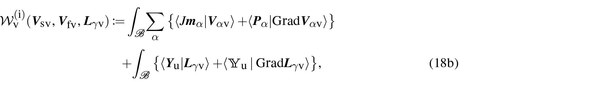
Given ${\mathcal{V}}_{\mathrm{sv}}$ , ${\mathcal{V}}_{\mathrm{fv}}$ and ${\mathcal{V}}_{\gamma \mathrm{v}}$ , we define the internal virtual power as

$$\begin{array}{ccc}\hfill & {\mathcal{W}}_{\mathrm{v}}^{(\mathrm{i})}:{\mathcal{V}}_{\mathrm{sv}}\times {\mathcal{V}}_{\mathrm{fv}}\times {\mathcal{V}}_{\gamma \mathrm{v}}\to \mathrm{ℝ},\hfill & \hfill \end{array}$$

(18a)

$$\begin{array}{cccc}\hfill & {\mathcal{W}}_{\mathrm{v}}^{(\mathrm{i})}({\mathit{V}}_{\mathrm{sv}},{\mathit{V}}_{\mathrm{fv}},{\mathit{L}}_{\gamma \mathrm{v}}):={\int }_{ℬ}\sum _{\alpha }\{⟨J{\mathit{m}}_{\alpha }|{\mathit{V}}_{\alpha \mathrm{v}}⟩+⟨{\mathit{P}}_{\alpha }|\mathrm{Grad}{\mathit{V}}_{\alpha \mathrm{v}}⟩\}\hfill & \hfill & \hfill \\ \hfill & +{\int }_{ℬ}\{⟨{\mathit{Y}}_{\mathrm{u}}|{\mathit{L}}_{\gamma \mathrm{v}}⟩+⟨{\mathbb{Y}}_{\mathrm{u}}|\mathrm{Grad}{\mathit{L}}_{\gamma \mathrm{v}}⟩\},\hfill & \hfill \end{array}$$

(18b)

where $J{\mathit{m}}_{\alpha }$ is the active part of the force, expressed per unit volume of the reference placement, that the αth phase, $\alpha \in \{\mathrm{s},\mathrm{f}\}$ , exchanges with the other one [55] (it is here referred to as “active” because it is not directly related to the constraints and, in the following, it will be expressed constitutively); ${\mathit{P}}_{\alpha }$ is the active part of the first Piola–Kirchhoff stress tensor associated with the αth phase; ${\mathit{Y}}_{\mathrm{u}}$ is the active stress-like generalized force dual to ${\mathit{L}}_{\gamma \mathrm{v}}$ ; finally, ${\mathbb{Y}}_{\mathrm{u}}$ is the tensor field of the third order that expresses the active generalized stress dual to $\mathrm{Grad}{\mathit{L}}_{\gamma \mathrm{v}}$ .

The generalized forces $J{\mathit{m}}_{\alpha }$ , ${\mathit{P}}_{\alpha }$ , ${\mathit{Y}}_{\mathrm{u}}$ and ${\mathbb{Y}}_{\mathrm{u}}$ must belong to functional spaces that guarantee the existence and finiteness of the integrals of equation (18b). Moreover, ${\mathcal{W}}_{\mathrm{v}}^{(\mathrm{i})}$ should be linear and bounded in each of its arguments.

3.1.2. Null reactive virtual power

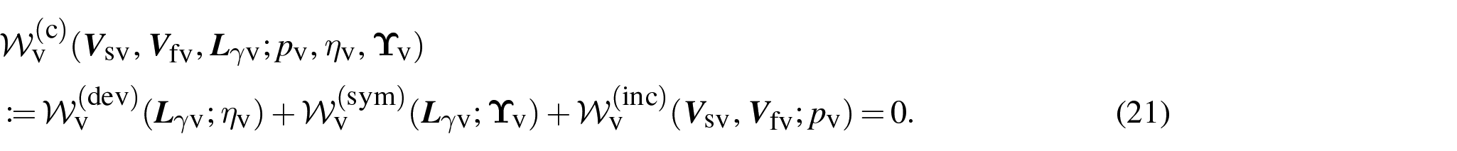
Since the constraints (10a) and (10b) are “ideal” [67,77], the reaction forces generated by them expend zero virtual power against any admissible virtual velocity field. We enforce this property weakly by employing the Lagrange multiplier technique. Hence, we introduce a scalar Lagrange multiplier η and a tensorial Lagrange multiplier Υ , their associated virtual fields ${\eta }_{\mathrm{v}}$ and ${\mathit{{\rm Y}}}_{\mathrm{v}}$ , and we conjugate ${\eta }_{\mathrm{v}}$ and ${\mathit{{\rm Y}}}_{\mathrm{v}}$ with equations (10a) and (10b), respectively, and η and Υ with Chetaev’s conditions (11a) and (11b). Note that η, ${\eta }_{\mathrm{v}}$ , Υ and ${\mathit{{\rm Y}}}_{\mathrm{v}}$ have physical units of mechanical stress.

Analogous considerations are made for the incompressibility constraint, expressed in the form (8b) and in Chetaev’s condition (15). The condition (15) is conjugated with a Lagrange multiplier p, acquiring the meaning of a pressure, while the constraint (8b) is conjugated with the virtual pressure $p_{\mathrm{v}}$ .

We denote by ${\mathcal{V}}_{\eta \mathrm{v}}$ , ${\mathcal{V}}_{\mathit{{\rm Y}}\mathrm{v}}$ , and ${\mathcal{V}}_{\mathrm{pv}}$ the functional spaces in which the virtual multipliers ${\eta }_{\mathrm{v}}$ , ${\mathit{{\rm Y}}}_{\mathrm{v}}$ , and $p_{\mathrm{v}}$ live, and we define them as

$$\begin{array}{ccccccc}\hfill & {\mathcal{V}}_{\eta \mathrm{v}}=L^2(ℬ;\mathrm{ℝ}),\hfill & \hfill & {\mathcal{V}}_{\mathit{{\rm Y}}\mathrm{v}}=L^2(ℬ;{[Tℬ]}^2),\hfill & \hfill & {\mathcal{V}}_{\mathrm{pv}}=H^1(ℬ;\mathrm{ℝ}).\hfill & \hfill \end{array}$$

(19)

Then, we write the null virtual powers expended by the reaction forces on the constraints as

$$\begin{array}{ccc}\hfill & {\mathcal{W}}_{\mathrm{v}}^{(\mathrm{dev})}:{\mathcal{V}}_{\gamma \mathrm{v}}\times {\mathcal{V}}_{\eta \mathrm{v}}\to \mathrm{ℝ},\hfill & \hfill \end{array}$$

(20a)

$$\begin{array}{ccc}\hfill & {\mathcal{W}}_{\mathrm{v}}^{(\mathrm{dev})}({\mathit{L}}_{\gamma \mathrm{v}};{\eta }_{\mathrm{v}}):={\int }_{ℬ}\eta [{\hat{\mathcal{A}}}_{\mathrm{dev}}\circ {\mathit{L}}_{\gamma \mathrm{v}}]+{\int }_{ℬ}{\eta }_{\mathrm{v}}[{\hat{\mathcal{C}}}_{\mathrm{dev}}\circ {\mathit{L}}_{\gamma }]=0,\hfill & \hfill \end{array}$$

(20b)

$$\begin{array}{ccc}\hfill & {\mathcal{W}}_{\mathrm{v}}^{(\mathrm{sym})}:{\mathcal{V}}_{\gamma \mathrm{v}}\times {\mathcal{V}}_{\mathit{{\rm Y}}\mathrm{v}}\to \mathrm{ℝ},\hfill & \hfill \end{array}$$

(20c)

$$\begin{array}{ccc}\hfill & {\mathcal{W}}_{\mathrm{v}}^{(\mathrm{sym})}({\mathit{L}}_{\gamma \mathrm{v}};{\mathit{{\rm Y}}}_{\mathrm{v}}):={\int }_{ℬ}⟨\mathit{{\rm Y}}|{\hat{\mathcal{A}}}_{\mathrm{sym}}\circ {\mathit{L}}_{\gamma \mathrm{v}}⟩+{\int }_{ℬ}⟨{\mathit{{\rm Y}}}_{\mathrm{v}}|{\hat{\mathcal{C}}}_{\mathrm{sym}}\circ {\mathit{L}}_{\gamma }⟩=0,\hfill & \hfill \end{array}$$

(20d)

$$\begin{array}{ccc}\hfill & {\mathcal{W}}_{\mathrm{v}}^{(\mathrm{inc})}:{\mathcal{V}}_{\mathrm{sv}}\times {\mathcal{V}}_{\mathrm{fv}}\times {\mathcal{V}}_{\mathrm{pv}}\to \mathrm{ℝ},\hfill & \hfill \end{array}$$

(20e)

$$\begin{array}{ccc}\hfill & {\mathcal{W}}_{\mathrm{v}}^{(\mathrm{inc})}({\mathit{V}}_{\mathrm{sv}},{\mathit{V}}_{\mathrm{fv}};p_{\mathrm{v}}):=-{\int }_{ℬ}p[{\hat{\mathcal{A}}}_{\mathrm{inc}}\circ ({\mathit{V}}_{\mathrm{sv}},{\mathit{V}}_{\mathrm{fv}})]-{\int }_{ℬ}{p}_{\mathrm{v}}[{\hat{\mathcal{C}}}_{\mathrm{inc}}\circ ({\mathit{V}}_{\mathrm{s}},{\mathit{V}}_{\mathrm{f}})]=0.\hfill & \hfill \end{array}$$

(20f)

As for ${\mathcal{W}}_{\mathrm{v}}^{(\mathrm{i})}$ , the functional spaces of the “true” Lagrange multipliers η, Υ and p, of the “true” velocity fields ${\mathit{V}}_{\mathrm{s}}$ and ${\mathit{V}}_{\mathrm{f}}$ , and of the motion χ must be such that the integrals in equations (20b), (20d) and (20f) exist and be finite. Moreover, the total (null) virtual power done by the reaction forces on the constraints is linear and bounded in its arguments and is given by

$$\begin{array}{cccc}\hfill & {\mathcal{W}}_{\mathrm{v}}^{(\mathrm{c})}({\mathit{V}}_{\mathrm{sv}},{\mathit{V}}_{\mathrm{fv}},{\mathit{L}}_{\gamma \mathrm{v}};p_{\mathrm{v}},{\eta }_{\mathrm{v}},{\mathit{{\rm Y}}}_{\mathrm{v}})\hfill & \hfill & \hfill \\ \hfill & :={\mathcal{W}}_{\mathrm{v}}^{(\mathrm{dev})}({\mathit{L}}_{\gamma \mathrm{v}};{\eta }_{\mathrm{v}})+{\mathcal{W}}_{\mathrm{v}}^{(\mathrm{sym})}({\mathit{L}}_{\gamma \mathrm{v}};{\mathit{{\rm Y}}}_{\mathrm{v}})+{\mathcal{W}}_{\mathrm{v}}^{(\mathrm{inc})}({\mathit{V}}_{\mathrm{sv}},{\mathit{V}}_{\mathrm{fv}};p_{\mathrm{v}})=0.\hfill & \hfill \end{array}$$

(21)

Although equations (20b) and (20d) state that the virtual power done by the reaction forces is zero, η and Υ are not the reaction forces, in general. They are, however, related to these forces, as will become clear in equations (22a) and (22b) below. Note also that, since ${\eta }_{\mathrm{v}}$ and ${\mathit{{\rm Y}}}_{\mathrm{v}}$ can be taken arbitrarily (see the forthcoming calculations), the last summands of equations (20b) and (20d) return the constraints (10a) and (10b) in strong form. Moreover, if the last integrals of equations (20b) and (20d) are evaluated for the “true” values of ${\mathit{L}}_{\gamma }$ , i.e., for the velocities solving the dynamic problem under study, which have to fulfill the constraints, then ${\hat{\mathcal{C}}}_{\mathrm{dev}}\circ {\mathit{L}}_{\gamma }$ and ${\hat{\mathcal{C}}}_{\mathrm{sym}}\circ {\mathit{L}}_{\gamma }$ vanish identically. The same holds true for the velocities ${\mathit{V}}_{\mathrm{s}}$ and ${\mathit{V}}_{\mathrm{f}}$ in the last integral of equation (20f).

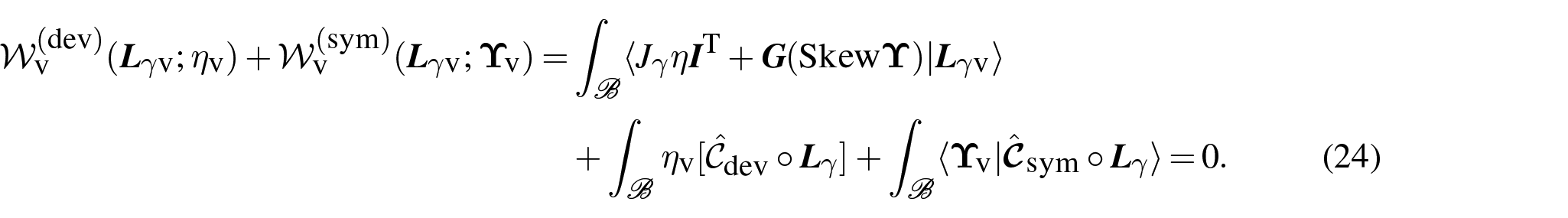
To identify explicitly the reaction forces associated with the constraints on ${\mathit{L}}_{\gamma }$ , let us rewrite the integrands $\eta [{\hat{\mathcal{A}}}_{\mathrm{dev}}\circ {\mathit{L}}_{\gamma \mathrm{v}}]$ and $⟨\mathit{{\rm Y}}|{\hat{\mathcal{A}}}_{\mathrm{sym}}\circ {\mathit{L}}_{\gamma \mathrm{v}}⟩$ in equations (20b) and (20d) as

$$\begin{array}{ccc}\hfill & \eta [{\hat{\mathcal{A}}}_{\mathrm{dev}}\circ {\mathit{L}}_{\gamma \mathrm{v}}]=⟨J_{\gamma }\eta {\mathit{I}}^{\mathrm{T}}|{\mathit{L}}_{\gamma \mathrm{v}}⟩=0,\hfill & \hfill \end{array}$$

(22a)

$$\begin{array}{ccc}\hfill & ⟨\mathit{{\rm Y}}|{\hat{\mathcal{A}}}_{\mathrm{sym}}\circ {\mathit{L}}_{\gamma \mathrm{v}}⟩=⟨\mathit{G}(\mathrm{Skew}\mathit{{\rm Y}})|{\mathit{L}}_{\gamma \mathrm{v}}⟩=0.\hfill & \hfill \end{array}$$

(22b)

These expressions make it clear that the reaction forces are dual to ${\mathit{L}}_{\gamma \mathrm{v}}$ and are represented by the tensor fields $J_{\gamma }\eta {\mathit{I}}^{\mathrm{T}}$ and $\mathit{G}(\mathrm{Skew}\mathit{{\rm Y}})$ . These quantities, in turn, viewed as real-valued linear maps acting on ${\mathcal{V}}_{\gamma \mathrm{v}}$ , read $⟨J_{\gamma }\eta {\mathit{I}}^{\mathrm{T}}|\cdot ⟩$ and $⟨\mathit{G}(\mathrm{Skew}\mathit{{\rm Y}})|\cdot ⟩$ . Consistently with this picture, the generalized virtual velocities ${\mathit{L}}_{\gamma \mathrm{v}}$ must belong to the intersection of the kernels of $⟨J_{\gamma }\eta {\mathit{I}}^{\mathrm{T}}|\cdot ⟩$ and $⟨\mathit{G}(\mathrm{Skew}\mathit{{\rm Y}})|\cdot ⟩$ . Hence, we write

$$\begin{array}{ccc}\hfill {\mathit{L}}_{\gamma \mathrm{v}}\in \mathrm{Ker}⟨J_{\gamma }\eta {\mathit{I}}^{\mathrm{T}}|\cdot ⟩\cap \mathrm{Ker}⟨\mathit{G}(\mathrm{Skew}\mathit{{\rm Y}})|\cdot ⟩,& \hfill & \hfill \end{array}$$

(23)

which implies that a generic ${\mathit{L}}_{\gamma \mathrm{v}}$ is admissible if it is deviatoric and symmetric with respect to the metric tensor field G . These conditions are prescribed on ${\mathit{L}}_{\gamma }$ by the constraints (10a) and (10b), and allow us to rewrite the first two summands on the right-hand side of equation (21) as

$$\begin{array}{cccc}\hfill {\mathcal{W}}_{\mathrm{v}}^{(\mathrm{dev})}({\mathit{L}}_{\gamma \mathrm{v}};{\eta }_{\mathrm{v}})+{\mathcal{W}}_{\mathrm{v}}^{(\mathrm{sym})}({\mathit{L}}_{\gamma \mathrm{v}};{\mathit{{\rm Y}}}_{\mathrm{v}})=& {\int }_{ℬ}⟨J_{\gamma }\eta {\mathit{I}}^{\mathrm{T}}+\mathit{G}(\mathrm{Skew}\mathit{{\rm Y}})|{\mathit{L}}_{\gamma \mathrm{v}}⟩\hfill & \hfill & \hfill \\ \hfill & +{\int }_{ℬ}{\eta }_{\mathrm{v}}[{\hat{\mathcal{C}}}_{\mathrm{dev}}\circ {\mathit{L}}_{\gamma }]+{\int }_{ℬ}⟨{\mathit{{\rm Y}}}_{\mathrm{v}}|{\hat{\mathcal{C}}}_{\mathrm{sym}}\circ {\mathit{L}}_{\gamma }⟩=0.\hfill & \hfill \end{array}$$

(24)

On the same footing, we can determine the reaction forces associated with the Lagrange multiplier p by working out the first integrand on the right-hand side of equation (20f). Indeed, by expanding the divergence in ${\hat{\mathcal{A}}}_{\mathrm{inc}}\circ ({\mathit{V}}_{\mathrm{sv}},{\mathit{V}}_{\mathrm{fv}})$ , and using the Piola identity, we obtain

$$\begin{array}{cccc}\hfill {\mathcal{W}}_{\mathrm{v}}^{(\mathrm{inc})}({\mathit{V}}_{\mathrm{sv}},{\mathit{V}}_{\mathrm{fv}};p_{\mathrm{v}})=& {\int }_{ℬ}\sum _{\alpha }\{⟨-\mathrm{Jp}{\mathit{F}}^{-\mathrm{T}}\mathrm{Grad}{\varphi }_{\alpha \mathrm{R}}|{\mathit{V}}_{\alpha \mathrm{v}}⟩+⟨-{\mathrm{\Phi }}_{\alpha \mathrm{R}}p{\mathit{F}}^{-\mathrm{T}}|\mathrm{Grad}{\mathit{V}}_{\alpha \mathrm{v}}⟩\}\hfill & \hfill & \hfill \end{array}$$

$$\begin{array}{ccc}\hfill & -{\int }_{ℬ}{p}_{\mathrm{v}}[{\hat{\mathcal{C}}}_{\mathrm{inc}}\circ ({\mathit{V}}_{\mathrm{s}},{\mathit{V}}_{\mathrm{f}})],\hfill & \hfill \end{array}$$

(25)

where ${\varphi }_{\alpha \mathrm{R}}\equiv {\varphi }_{\alpha }\circ (\chi ,\mathcal{T})={\mathrm{\Phi }}_{\alpha \mathrm{R}}∕J$ . Hence, for $\alpha =\mathrm{s}\mathrm{,}\mathrm{f}$ , we identify the reactive contributions

$$\begin{array}{ccccc}\hfill & -\mathrm{Jp}{\mathit{F}}^{-\mathrm{T}}\mathrm{Grad}{\varphi }_{\alpha \mathrm{R}}\equiv -\mathrm{Jp}[\mathrm{grad}{\varphi }_{\alpha }\circ (\chi ,\mathcal{T})],\hfill & \hfill & -{\mathrm{\Phi }}_{\alpha \mathrm{R}}p{\mathit{F}}^{-\mathrm{T}}.\hfill & \hfill \end{array}$$

(26)

The force in equation (26)₁ is the reaction part of the internal force due to the momentum exchange between the solid and the fluid phase of the considered medium. For $\alpha =\mathrm{s}\mathrm{,}\mathrm{f}$ , $-\mathrm{Jp}{\mathit{F}}^{-\mathrm{T}}\mathrm{Grad}{\varphi }_{\alpha \mathrm{R}}$ adds to $J{\mathit{m}}_{\alpha }$ to determine the overall internal force dual to ${\mathit{V}}_{\alpha \mathrm{v}}$ . Moreover, it satisfies the requirement that the sum over $\alpha =\mathrm{s}\mathrm{,}\mathrm{f}$ of the internal forces should be null. This follows from the saturation condition ${\mathrm{\sum }}_{\alpha }{\varphi }_{\alpha \mathrm{R}}=1$ , which yields $-{\mathrm{\sum }}_{\alpha }\mathrm{Jp}{\mathit{F}}^{-\mathrm{T}}\mathrm{Grad}{\varphi }_{\alpha \mathrm{R}}=-\mathrm{Jp}{\mathit{F}}^{-\mathrm{T}}\mathrm{Grad}({\sum }_{\alpha }{\varphi }_{\alpha \mathrm{R}})=\mathit{0}$ . Similarly, the stress contribution $-{\mathrm{\Phi }}_{\alpha \mathrm{R}}p{\mathit{F}}^{-\mathrm{T}}$ in equation (26)₂ identifies the reaction part of the first Piola–Kirchhoff stress tensor of the αth phase dual to the gradient $\mathrm{Grad}{\mathit{V}}_{\alpha \mathrm{v}}$ of the corresponding virtual velocity.

3.1.3. External virtual power

Next, we define the external virtual power as

$$\begin{array}{ccc}\hfill & {\mathcal{W}}_{\mathrm{v}}^{(\mathrm{e})}:{\mathcal{V}}_{\mathrm{sv}}\times {\mathcal{V}}_{\mathrm{fv}}\times {\mathcal{V}}_{\gamma \mathrm{v}}\to \mathrm{ℝ},\hfill & \hfill \end{array}$$

(27a)

$$\begin{array}{ccc}\hfill & {\mathcal{W}}_{\mathrm{v}}^{(\mathrm{e})}({\mathit{V}}_{\mathrm{sv}},{\mathit{V}}_{\mathrm{fv}},{\mathit{L}}_{\gamma \mathrm{v}}):={\int }_{ℬ}\sum _{\alpha }⟨{\mathit{f}}_{\alpha }|{\mathit{V}}_{\alpha \mathrm{v}}⟩+\sum _{\alpha }\sum _{d=1}^3{\int }_{\mathrm{\partial ℬ}\setminus {\mathrm{\Gamma }}_{\alpha \mathrm{D}}^d}{\tau }_{\mathrm{\alpha d}}{V}_{\alpha \mathrm{v}}^d+{\int }_{ℬ}⟨\mathit{Z}|{\mathit{L}}_{\gamma \mathrm{v}}⟩,\hfill & \hfill \end{array}$$

(27b)

where ${\mathit{f}}_{\alpha }:={\mathrm{\Phi }}_{\alpha \mathrm{R}}{\varrho }_{\alpha }\mathit{f}$ is the amount of the external force per unit mass f felt by the αth phase [55]; ${\tau }_{\mathrm{\alpha d}}$ is the dth component, in the given basis of co-vector fields ${\{{\mathit{e}}^c\}}_{c=1}^3\subset {(T\mathcal{S})}^{\ast }$ , of the contact force ${\mathit{\tau }}_{\alpha }$ , relative to the αth phase, that is assumed to act on the portion of $\mathrm{\partial ℬ}$ complementary to ${\mathrm{\Gamma }}_{\alpha \mathrm{D}}^d$ (see Hughes [81]); Z is the external force density associated with the remodeling process acting on the remodeling rate ${\mathit{L}}_{\gamma }$ . The forces ${\mathit{f}}_{\alpha }$ , ${\mathit{\tau }}_{\alpha }$ , and Z must guarantee the existence and finiteness of the integrals in equation (27b), and ${\mathcal{W}}_{\mathrm{v}}^{(\mathrm{e})}$ must be linear and bounded in each of its arguments. Moreover, we assume negligible inertial forces and no external forces dual to the functional trace of the virtual remodeling rate on $\mathrm{\partial ℬ}$ . It is worth emphasizing that, as evidenced by Gurtin and Anand [38], one could also account for an additional supply of external work manifested in the form of “remodeling” contact forces operating on the boundary $\mathrm{\partial ℬ}$ . However, we do not introduce these external agencies here and, consequently, we restrict our investigation to what Gurtin and Anand [38] call “microscopically free” boundaries.

3.1.4. Principle of Virtual Power (PVP)

The definition (21) of ${\mathcal{W}}_{\mathrm{v}}^{(\mathrm{c})}$ as a useful tool for studying constrained systems by means of the PVP is taken from the book by Bonet and Wood [82], in which the PVP is formulated for computational problems. Following this methodology, we employ a constrained form of the PVP, which requires the fulfillment of the condition

$$\begin{array}{ccc}\hfill {\mathcal{W}}_{\mathrm{v}}^{(\mathrm{i})}({\mathit{V}}_{\mathrm{sv}},{\mathit{V}}_{\mathrm{fv}},{\mathit{L}}_{\gamma \mathrm{v}})+{\mathcal{W}}_{\mathrm{v}}^{(\mathrm{c})}({\mathit{V}}_{\mathrm{sv}},{\mathit{V}}_{\mathrm{fv}},{\mathit{L}}_{\gamma \mathrm{v}};p_{\mathrm{v}},{\eta }_{\mathrm{v}},{\mathit{{\rm Y}}}_{\mathrm{v}})={\mathcal{W}}_{\mathrm{v}}^{(\mathrm{e})}({\mathit{V}}_{\mathrm{sv}},{\mathit{V}}_{\mathrm{fv}},{\mathit{L}}_{\gamma \mathrm{v}})& \hfill & \hfill \end{array}$$

(28)

for all the triples $({\mathit{V}}_{\mathrm{sv}},{\mathit{V}}_{\mathrm{fv}},{\mathit{L}}_{\gamma \mathrm{v}})\in {\mathcal{V}}_{\mathrm{sv}}\times {\mathcal{V}}_{\mathrm{fv}}\times {\mathcal{V}}_{\gamma \mathrm{v}}$ and $(p_{\mathrm{v}},{\eta }_{\mathrm{v}},{\mathit{{\rm Y}}}_{\mathrm{v}})\in {\mathcal{V}}_{\mathrm{pv}}\times {\mathcal{V}}_{\eta \mathrm{v}}\times {\mathcal{V}}_{\mathit{{\rm Y}}\mathrm{v}}$ . A similar treatment of the constraints of the mixture incompressibility and of the isochoricity of the remodeling tensor is given in the work of Giammarini et al. [46].

From here on, we introduce the notation

$$\begin{array}{ccccc}\hfill & {\mathbf{\Pi }}_{\alpha }:=-{\mathrm{\Phi }}_{\alpha \mathrm{R}}p{\mathit{F}}^{-\mathrm{T}}+{\mathit{P}}_{\alpha },\hfill & \hfill & \alpha =\mathrm{s}\mathrm{,}\mathrm{f},\hfill & \hfill \end{array}$$

(29)

and, by invoking Gauss’ Theorem and Leibniz rule of differentiation, and recalling that the dth component of the virtual velocity ${\mathit{V}}_{\alpha \mathrm{v}}$ vanishes identically on ${\mathrm{\Gamma }}_{\alpha \mathrm{D}}^d$ , we recast equation (28) in the form

$$\begin{array}{cccc}\hfill & {\int }_{ℬ}\sum _{\alpha }⟨J{\mathit{m}}_{\alpha }-\mathrm{Jp}{\mathit{F}}^{-\mathrm{T}}\mathrm{Grad}{\varphi }_{\alpha \mathrm{R}}-\mathrm{Div}{\mathbf{\Pi }}_{\alpha }-{\mathrm{\Phi }}_{\alpha \mathrm{R}}{\varrho }_{\alpha }\mathit{f}|{\mathit{V}}_{\alpha \mathrm{v}}⟩\hfill & \hfill & \hfill \\ \hfill & +{\int }_{ℬ}⟨{\mathit{Y}}_{\mathrm{u}}+\eta J_{\gamma }{\mathit{I}}^{\mathrm{T}}+\mathit{G}(\mathrm{Skew}\mathit{{\rm Y}})-\mathrm{Div}{\mathbb{Y}}_{\mathrm{u}}-\mathit{Z}|{\mathit{L}}_{\gamma \mathrm{v}}⟩\hfill & \hfill & \hfill \\ \hfill & +\sum _{\alpha }\sum _{d=1}^3{\int }_{\mathrm{\partial ℬ}\setminus {\mathrm{\Gamma }}_{\alpha \mathrm{D}}^d}\{{[{\mathbf{\Pi }}_{\alpha }\mathit{N}]}_d-{\tau }_{\mathrm{\alpha d}}\}{V}_{\alpha \mathrm{v}}^d+{\int }_{\mathrm{\partial ℬ}}⟨{\mathbb{Y}}_{\mathrm{u}}\mathit{N}|{\mathit{L}}_{\gamma \mathrm{v}}⟩\hfill & \hfill & \hfill \\ \hfill & -{\int }_{ℬ}{p}_{\mathrm{v}}[{\hat{\mathcal{C}}}_{\mathrm{inc}}\circ ({\mathit{V}}_{\mathrm{s}},{\mathit{V}}_{\mathrm{f}})]+{\int }_{ℬ}{\eta }_{\mathrm{v}}[{\hat{\mathcal{C}}}_{\mathrm{dev}}\circ {\mathit{L}}_{\gamma }]+{\int }_{ℬ}⟨{\mathit{{\rm Y}}}_{\mathrm{v}}|{\hat{\mathcal{C}}}_{\mathrm{sym}}\circ {\mathit{L}}_{\gamma }⟩=0,\hfill & \hfill \end{array}$$

(30)

with ${[{\mathbf{\Pi }}_{\alpha }\mathit{N}]}_d={[{\mathbf{\Pi }}_{\alpha }{]}_d}^B{N}_B$ , and N being the field of co-normals associated with $\mathrm{\partial ℬ}$ . Finally, as shown in equation (22b), only the skew-symmetric part of Υ is accounted for in equation (30) because the symmetric part, $\mathrm{Sym}\mathit{{\rm Y}}$ , is filtered out by the duality product with ${\hat{\mathcal{A}}}_{\mathrm{sym}}\circ {\mathit{L}}_{\gamma \mathrm{v}}$ , which is a skew-symmetric tensor field.

To deduce equation (30), we first apply Leibniz rule to $⟨{\mathit{P}}_{\alpha }|\mathrm{Grad}{\mathit{V}}_{\alpha \mathrm{v}}⟩$ and $⟨{\mathbb{Y}}_{\mathrm{u}}|\mathrm{Grad}{\mathit{L}}_{\gamma \mathrm{v}}⟩$ in equation (18b) and to $⟨-{\mathrm{\Phi }}_{\alpha \mathrm{R}}p{\mathit{F}}^{-\mathrm{T}}|\mathrm{Grad}{\mathit{V}}_{\alpha \mathrm{v}}⟩$ in equation (25), i.e.,

$$\begin{array}{ccc}\hfill & ⟨{\mathit{P}}_{\alpha }|\mathrm{Grad}{\mathit{V}}_{\alpha \mathrm{v}}⟩=\mathrm{Div}({\mathit{P}}_{\alpha }^{\mathrm{T}}{\mathit{V}}_{\alpha \mathrm{v}})-⟨\mathrm{Div}{\mathit{P}}_{\alpha }|{\mathit{V}}_{\alpha \mathrm{v}}⟩,\hfill & \hfill \end{array}$$

(31a)

$$\begin{array}{ccc}\hfill & ⟨{\mathbb{Y}}_{\mathrm{u}}|\mathrm{Grad}{\mathit{L}}_{\gamma \mathrm{v}}⟩=\mathrm{Div}({\mathbb{Y}}_{\mathrm{u}}^{\mathrm{T}}:{\mathit{L}}_{\gamma \mathrm{v}})-⟨\mathrm{Div}{\mathbb{Y}}_{\mathrm{u}}|{\mathit{L}}_{\gamma \mathrm{v}}⟩,\hfill & \hfill \end{array}$$

(31b)

$$\begin{array}{ccc}\hfill & ⟨-{\mathrm{\Phi }}_{\alpha \mathrm{R}}p{\mathit{F}}^{-\mathrm{T}}|\mathrm{Grad}{\mathit{V}}_{\alpha \mathrm{v}}⟩=\mathrm{Div}(-{\mathrm{\Phi }}_{\alpha \mathrm{R}}p{\mathit{F}}^{-1}{\mathit{V}}_{\alpha \mathrm{v}})-⟨\mathrm{Div}(-{\mathrm{\Phi }}_{\alpha \mathrm{R}}p{\mathit{F}}^{-\mathrm{T}})|{\mathit{V}}_{\alpha \mathrm{v}}⟩.\hfill & \hfill \end{array}$$

(31c)

The transposed tensor ${\mathbb{Y}}_{\mathrm{u}}^{\mathrm{T}}$ in equation (31b) has components $[{\mathbb{Y}}_{\mathrm{u}}^{\mathrm{T}}{]}^L{M}^N$ (instead, ${\mathbb{Y}}_{\mathrm{u}}$ has indices placed as in ${[{\mathbb{Y}}_{\mathrm{u}}{]}_M}^{\mathrm{NL}}$ ) and ${\mathbb{Y}}_{\mathrm{u}}^{\mathrm{T}}:{\mathit{L}}_{\gamma \mathrm{v}}$ represents a pseudo-vector field with components ${[{\mathbb{Y}}_{\mathrm{u}}^{\mathrm{T}}:{\mathit{L}}_{\gamma \mathrm{v}}]}^A=[{\mathbb{Y}}_{\mathrm{u}}^{\mathrm{T}}{]}^A{B}^C{[{\mathit{L}}_{\gamma \mathrm{v}}{]}^B}_C$ .

The products ${[{\mathbf{\Pi }}_{\alpha }\mathit{N}]}_d{V}_{\alpha \mathrm{v}}^d$ (no summation over $d=1\mathrm{,}2\mathrm{,}3$ ) and $⟨{\mathbb{Y}}_{\mathrm{u}}\mathit{N}|{\mathit{L}}_{\gamma \mathrm{v}}⟩$ in the surface integrals over $\mathrm{\partial ℬ}\setminus {\mathrm{\Gamma }}_{\alpha \mathrm{D}}^d$ and $\mathrm{\partial ℬ}$ of equation (30) descend from the application of Gauss’ Theorem to $\mathrm{Div}({\mathbf{\Pi }}_{\alpha }^{\mathrm{T}}{\mathit{V}}_{\alpha \mathrm{v}})$ and $\mathrm{Div}({\mathbb{Y}}_{\mathrm{u}}^{\mathrm{T}}:{\mathit{L}}_{\gamma \mathrm{v}})$ , which arise by working out equation (28) and adding equations (31a) and (31c) term by term. On $\mathrm{\partial ℬ}\setminus {\mathrm{\Gamma }}_{\alpha \mathrm{D}}^d$ , the components $V_{\alpha \mathrm{v}}^d$ of the generalized virtual velocities need not vanish identically. Hence, we find:

$$\begin{array}{ccc}\hfill & {\int }_{ℬ}\sum _{\alpha }\mathrm{Div}({\mathbf{\Pi }}_{\alpha }^{\mathrm{T}}{\mathit{V}}_{\alpha \mathrm{v}})={\int }_{\mathrm{\partial ℬ}}\sum _{\alpha }⟨{\mathbf{\Pi }}_{\alpha }^{\mathrm{T}}{\mathit{V}}_{\alpha \mathrm{v}}|\mathit{N}⟩=\sum _{\alpha }\sum _{d=1}^3{\int }_{\mathrm{\partial ℬ}\setminus {\mathrm{\Gamma }}_{\alpha \mathrm{D}}^d}{[{\mathbf{\Pi }}_{\alpha }\mathit{N}]}_d{V}_{\alpha \mathrm{v}}^d,\hfill & \hfill \end{array}$$

(32a)

$$\begin{array}{ccc}\hfill & {\int }_{ℬ}\mathrm{Div}({\mathbb{Y}}_{\mathrm{u}}^{\mathrm{T}}:{\mathit{L}}_{\gamma \mathrm{v}})={\int }_{\mathrm{\partial ℬ}}⟨{\mathbb{Y}}_{\mathrm{u}}^{\mathrm{T}}:{\mathit{L}}_{\gamma \mathrm{v}}|\mathit{N}⟩={\int }_{\mathrm{\partial ℬ}}⟨{\mathbb{Y}}_{\mathrm{u}}\mathit{N}|{\mathit{L}}_{\gamma \mathrm{v}}⟩,\hfill & \hfill \end{array}$$

(32b)

where we used the identities $⟨{\mathbf{\Pi }}_{\alpha }^{\mathrm{T}}{\mathit{V}}_{\alpha \mathrm{v}}|\mathit{N}⟩\equiv ⟨{\mathbf{\Pi }}_{\alpha }\mathit{N}|{\mathit{V}}_{\alpha \mathrm{v}}⟩$ and $⟨{\mathbb{Y}}_{\mathrm{u}}^{\mathrm{T}}:{\mathit{L}}_{\gamma \mathrm{v}}|\mathit{N}⟩\equiv ⟨{\mathbb{Y}}_{\mathrm{u}}\mathit{N}|{\mathit{L}}_{\gamma \mathrm{v}}⟩$ .

To obtain equations (30), (32a), and (32b), we have adapted a result of Functional Analysis (see Corollary 7.1, page 413 of the book by Salsa [80]), which requires ${\mathbf{\Pi }}_{\alpha }\in H^1(ℬ;{(T\mathcal{S})}^{\ast }\otimes Tℬ)$ and ${\mathbb{Y}}_{\mathrm{u}}\in H^1(ℬ;{[Tℬ{]}_1}^2)$ . This implies $-\mathrm{Div}{\mathbf{\Pi }}_{\alpha }\in L^2(ℬ;{(T\mathcal{S})}^{\ast })$ and $-\mathrm{Div}{\mathbb{Y}}_{\mathrm{u}}\in L^2(ℬ;{[Tℬ{]}_1}^1)$ .

3.2. Strong form of the problem of the remodeling of biphasic mixtures

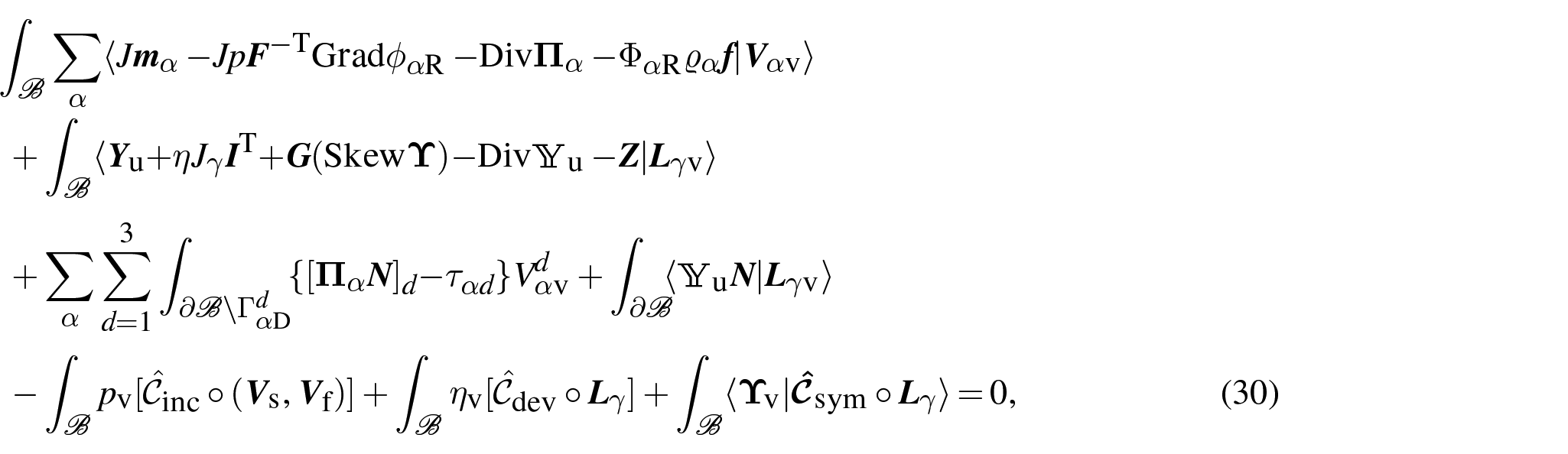
Starting from equation (30), classical localization procedures yield the force balances and the constraints of the system under consideration in local form, i.e.,

$$\begin{array}{ccccc}\hfill & J{\mathit{m}}_{\mathrm{s}}-\mathrm{Jp}{\mathit{F}}^{-\mathrm{T}}\mathrm{Grad}{\varphi }_{\mathrm{sR}}-\mathrm{Div}(-{\mathrm{\Phi }}_{\mathrm{sR}}p{\mathit{F}}^{-\mathrm{T}}+{\mathit{P}}_{\mathrm{s}})-{\mathit{f}}_{\mathrm{s}}=\mathbf{0},\hfill & \hfill & \mathrm{in}ℬ,\hfill & \hfill \end{array}$$

(33a)

$$\begin{array}{ccccc}\hfill & J{\mathit{m}}_{\mathrm{f}}-\mathrm{Jp}{\mathit{F}}^{-\mathrm{T}}\mathrm{Grad}{\varphi }_{\mathrm{fR}}-\mathrm{Div}(-{\mathrm{\Phi }}_{\mathrm{fR}}p{\mathit{F}}^{-\mathrm{T}}+{\mathit{P}}_{\mathrm{f}})-{\mathit{f}}_{\mathrm{f}}=\mathbf{0},\hfill & \hfill & \mathrm{in}ℬ,\hfill & \hfill \end{array}$$

(33b)

$$\begin{array}{ccccc}\hfill & {[(-{\mathrm{\Phi }}_{\mathrm{sR}}p{\mathit{F}}^{-\mathrm{T}}+{\mathit{P}}_{\mathrm{s}})\mathit{N}]}_d={\tau }_{\mathrm{s}d},\hfill & \hfill & \mathrm{on}\mathrm{\partial ℬ}\setminus {\mathrm{\Gamma }}_{\mathrm{sD}}^d,d=1,2,3,\hfill & \hfill \end{array}$$

(33c)

$$\begin{array}{ccccc}\hfill & {[(-{\mathrm{\Phi }}_{\mathrm{fR}}p{\mathit{F}}^{-\mathrm{T}}+{\mathit{P}}_{\mathrm{f}})\mathit{N}]}_d={\tau }_{\mathrm{f}d},\hfill & \hfill & \mathrm{on}\mathrm{\partial ℬ}\setminus {\mathrm{\Gamma }}_{\mathrm{fD}}^d,d=1,2,3,\hfill & \hfill \end{array}$$

(33d)

$$\begin{array}{ccccc}\hfill & {\mathit{Y}}_{\mathrm{u}}+\eta J_{\gamma }{\mathit{I}}^{\mathrm{T}}+\mathit{G}(\mathrm{Skew}\mathit{{\rm Y}})-\mathrm{Div}{\mathbb{Y}}_{\mathrm{u}}-\mathit{Z}=\mathit{O},\hfill & \hfill & \mathrm{in}ℬ,\hfill & \hfill \end{array}$$

(33e)

$$\begin{array}{ccccc}\hfill & {\mathbb{Y}}_{\mathrm{u}}\mathit{N}=\mathit{O},\hfill & \hfill & \mathrm{on}\mathrm{\partial ℬ},\hfill & \hfill \end{array}$$

(33f)

$$\begin{array}{ccccc}\hfill & {\hat{\mathcal{C}}}_{\mathrm{inc}}\circ ({\mathit{V}}_{\mathrm{s}},{\mathit{V}}_{\mathrm{f}})=\mathrm{Div}[({\mathrm{\Phi }}_{\mathrm{sR}}{\mathit{V}}_{\mathrm{s}}+{\mathrm{\Phi }}_{\mathrm{fR}}{\mathit{V}}_{\mathrm{f}}){\mathit{F}}^{-\mathrm{T}}]=0,\hfill & \hfill & \mathrm{in}ℬ,\hfill & \hfill \end{array}$$

(33g)

$$\begin{array}{ccccc}\hfill & {\hat{\mathcal{C}}}_{\mathrm{dev}}\circ {\mathit{L}}_{\gamma }=⟨J_{\gamma }{\mathit{I}}^{\mathrm{T}}|{\mathit{L}}_{\gamma }⟩=J_{\gamma }\mathrm{tr}{\mathit{L}}_{\gamma }=0,\hfill & \hfill & \mathrm{in}ℬ,\hfill & \hfill \end{array}$$

(33h)

$$\begin{array}{ccccc}\hfill & {\hat{\mathcal{C}}}_{\mathrm{sym}}\circ {\mathit{L}}_{\gamma }=\frac{1}{2}[\mathit{G}{\mathit{L}}_{\gamma }-{(\mathit{G}{\mathit{L}}_{\gamma })}^{\mathrm{T}}]=\mathit{O},\hfill & \hfill & \mathrm{in}ℬ.\hfill & \hfill \end{array}$$

(33i)

Aside from the natural boundary conditions (33c), (33d) and (33f), the system (33a)–(33i) yields 20 independent scalar equations and features 80 unknown scalars fields: 20 of these are given by the basic kinematic variables χ, ${\mathit{V}}_{\mathrm{f}}$ , and ${\mathit{F}}_{\gamma }$ (15 scalar unknowns) and by the Lagrange multipliers p, η, and $\mathrm{Skew}\mathit{{\rm Y}}$ (5 scalar unknowns), while the remaining 60 unknowns are the components of the fields ${\mathit{m}}_{\mathrm{s}}$ , ${\mathit{m}}_{\mathrm{f}}$ , ${\mathit{P}}_{\mathrm{s}}$ , ${\mathit{P}}_{\mathrm{f}}$ , ${\mathit{Y}}_{\mathrm{u}}$ , and ${\mathbb{Y}}_{\mathrm{u}}$ . We recall that ${\mathrm{\Phi }}_{\mathrm{sR}}$ is regarded as known, while ${\mathrm{\Phi }}_{\mathrm{fR}}=J-{\mathrm{\Phi }}_{\mathrm{sR}}$ , ${\varphi }_{\mathrm{sR}}={\mathrm{\Phi }}_{\mathrm{sR}}∕J$ , and ${\varphi }_{\mathrm{fR}}={\mathrm{\Phi }}_{\mathrm{fR}}∕J$ are expressed as functions of J, as per equation (7)₁. Similar considerations have recently been done in the work by Giammarini et al. [46]. Moreover, equation (33e) splits as

$$\begin{array}{ccc}\hfill & \eta =-\frac{1}{3}\mathrm{tr}[J_{\gamma }^{-1}({\mathit{Y}}_{\mathrm{u}}-\mathrm{Div}{\mathbb{Y}}_{\mathrm{u}}-\mathit{Z})],\hfill & \hfill \end{array}$$

(34a)

$$\begin{array}{ccc}\hfill & \mathrm{Skew}\mathit{{\rm Y}}=-\mathrm{Skew}[{\mathit{G}}^{-1}({\mathit{Y}}_{\mathrm{u}}-\mathrm{Div}{\mathbb{Y}}_{\mathrm{u}}-\mathit{Z})],\hfill & \hfill \end{array}$$

(34b)

$$\begin{array}{ccc}\hfill & {\mathrm{Dev}}_{\mathit{G}}\mathrm{Sym}[{\mathit{G}}^{-1}({\mathit{Y}}_{\mathrm{u}}-\mathrm{Div}{\mathbb{Y}}_{\mathrm{u}}-\mathit{Z})]=\mathit{O},\hfill & \hfill \end{array}$$

(34c)

with ${\mathrm{Dev}}_{\mathit{G}}\mathit{A}:=\mathit{A}-\frac{1}{3}⟨\mathit{G}|\mathit{A}⟩{\mathit{G}}^{-1}$ , for any $\mathit{A}=A^{\mathrm{MN}}{\mathit{E}}_M\otimes {\mathit{E}}_N$ , $\mathit{A}={\mathit{A}}^{\mathrm{T}}$ (see Grillo and Di Stefano [34,83] and Giammarini et al. [46]). Hence, η and $\mathrm{Skew}\mathit{{\rm Y}}$ can be computed separately, and the balance law (34c), which is equivalent to 5 scalar equations, replaces (33e) in the system (33a)–(33i). This reduces the number of coupled scalar equations to 16 and the number of effective unknowns to 76. However, granted the restrictions ${\mathit{m}}_{\mathrm{s}}+{\mathit{m}}_{\mathrm{f}}=\mathit{0}$ and ${\mathit{g}}^{-1}{\mathit{P}}_{\alpha }{\mathit{F}}^{\mathrm{T}}={({\mathit{g}}^{-1}{\mathit{P}}_{\alpha }{\mathit{F}}^{\mathrm{T}})}^{\mathrm{T}}$ , for $\alpha =\mathrm{s}\mathrm{,}\mathrm{f}$ , which originate from the invariance of the internal virtual power under the superposition of arbitrary translational and rotational rigid motions [44,55], the fields ${\mathit{m}}_{\mathrm{f}}$ , ${\mathit{P}}_{\mathrm{s}}$ , ${\mathit{P}}_{\mathrm{f}}$ , ${\mathit{Y}}_{\mathrm{u}}$ , and ${\mathbb{Y}}_{\mathrm{u}}$ will be assigned constitutively, thereby providing 60 scalar constitutive functions.

4. Constitutive assignments

For brevity, we concentrate on the consistency of the constitutive relations with objectivity and with the dissipation inequality of the system under study, while we give for granted all the other axioms of the general theory of constitutive laws [84]. Following Cermelli and Gurtin [63] and Gurtin and Anand [38], some constitutive functions depend solely on the remodeling descriptors ${\mathit{F}}_{\gamma }$ and $\mathrm{Curl}{\mathit{F}}_{\gamma }$ , and are defined so as to be invariant under smooth transformations of the reference placement of the system.

4.1. Dissipation inequality

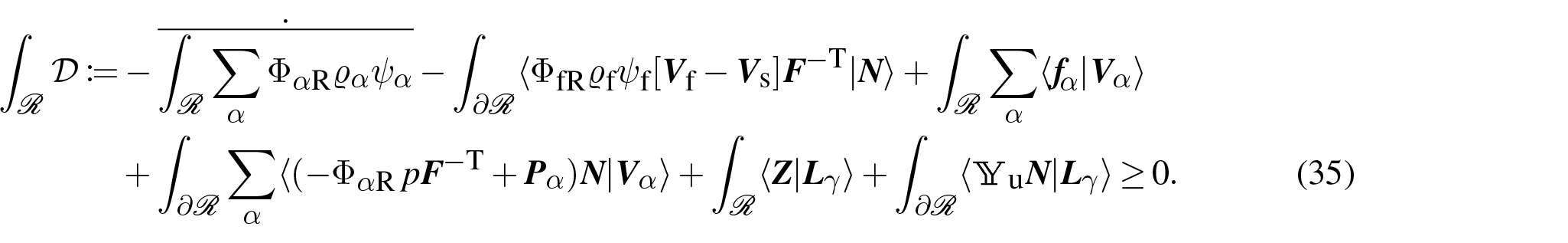
By adapting the approaches of Cermelli and Gurtin [63], Cermelli et al. [85], and Gurtin and Anand [38] to biphasic mixtures, we consider a fixed region $ℛ\subset ℬ$ and the Helmholtz free energy density ${\psi }_{\alpha }$ of the αth phase, with $\alpha =\mathrm{s}\mathrm{,}\mathrm{f}$ , per unit mass of the same phase. Then, we write the dissipation inequality:

$$\begin{array}{cccc}\hfill {\int }_{ℛ}\mathcal{D}:=& -\stackrel{·}{\overline{{\int }_{ℛ}\sum _{\alpha }{\mathrm{\Phi }}_{\alpha \mathrm{R}}{\varrho }_{\alpha }{\psi }_{\alpha }}}-{\int }_{\mathrm{\partial ℛ}}⟨{\mathrm{\Phi }}_{\mathrm{fR}}{\varrho }_{\mathrm{f}}{\psi }_{\mathrm{f}}[{\mathit{V}}_{\mathrm{f}}-{\mathit{V}}_{\mathrm{s}}]{\mathit{F}}^{-\mathrm{T}}|\mathit{N}⟩+{\int }_{ℛ}\sum _{\alpha }⟨{\mathit{f}}_{\alpha }|{\mathit{V}}_{\alpha }⟩\hfill & \hfill & \hfill \\ \hfill & +{\int }_{\mathrm{\partial ℛ}}\sum _{\alpha }⟨(-{\mathrm{\Phi }}_{\alpha \mathrm{R}}p{\mathit{F}}^{-\mathrm{T}}+{\mathit{P}}_{\alpha })\mathit{N}|{\mathit{V}}_{\alpha }⟩+{\int }_{ℛ}⟨\mathit{Z}|{\mathit{L}}_{\gamma }⟩+{\int }_{\mathrm{\partial ℛ}}⟨{\mathbb{Y}}_{\mathrm{u}}\mathit{N}|{\mathit{L}}_{\gamma }⟩\ge 0.\hfill & \hfill \end{array}$$

(35)

Given a region $ℛ(t)\subset ℬ(t)$ contained in the current placement of the system, and the spatial (or Eulerian) representation of an $\mathbb{S}$ -valued field ${}^{e}f:ℛ(t)\times \mathcal{T}\to \mathbb{S}$ , where $\mathbb{S}$ is ℝ or any vector or tensor space, we define $f:={}^{e}f\circ (\chi ,\mathcal{T}):ℛ\times \mathcal{T}\to \mathbb{S}$ , with $ℛ={[\hat{\chi }(\cdot ,t)]}^{-1}(ℛ(t))\subset ℬ$ and ${[\hat{\chi }(\cdot ,t)]}^{-1}\equiv {\hat{\chi }}_t^{-1}$ . Hence, the time derivative of the integral of f over ℛ reads

$$\begin{array}{ccccc}\hfill & \stackrel{·}{\overline{{\int }_{ℛ}f}}={\int }_{ℛ}ḟ,\hfill & \hfill & \mathrm{with}ḟ=(D_{\mathrm{s}}{}^{e}f)\circ (\chi ,\mathcal{T})\equiv [{\partial }_t{}^{e}f+(\mathrm{grad}{}^{e}f){\mathit{v}}_{\mathrm{s}}]\circ (\chi ,\mathcal{T}).\hfill & \hfill \end{array}$$

(36)

The quantity $ḟ=(D_{\mathrm{s}}{}^{e}f)\circ (\chi ,\mathcal{T})$ is the time derivative of ${}^{e}f$ with respect to the solid phase motion.

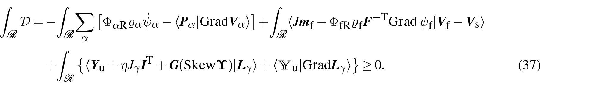
The second term on the right-hand side of equation (35) compensates for the fact that, in the first term, the derivative of ${\mathrm{\Phi }}_{\alpha \mathrm{R}}{\varrho }_{\alpha }{\psi }_{\alpha }$ is taken with respect to the velocity of the solid phase even for $\alpha =\mathrm{f}$ . Then, by working out the time derivatives, and invoking Gauss’ Theorem, the mass balances, ¹ the incompressibility constraint (8b), the force balances (33a) and (33b), and the condition ${\mathit{m}}_{\mathrm{s}}+{\mathit{m}}_{\mathrm{f}}=\mathbf{0}$ , we obtain

$$\begin{array}{cccc}\hfill {\int }_{ℛ}\mathcal{D}=& -{\int }_{ℛ}\sum _{\alpha }[{\mathrm{\Phi }}_{\alpha \mathrm{R}}{\varrho }_{\alpha }{\stackrel{·}{\psi }}_{\alpha }-⟨{\mathit{P}}_{\alpha }|\mathrm{Grad}{\mathit{V}}_{\alpha }⟩]+{\int }_{ℛ}⟨J{\mathit{m}}_{\mathrm{f}}-{\mathrm{\Phi }}_{\mathrm{fR}}{\varrho }_{\mathrm{f}}{\mathit{F}}^{-\mathrm{T}}\mathrm{Grad}{\psi }_{\mathrm{f}}|{\mathit{V}}_{\mathrm{f}}-{\mathit{V}}_{\mathrm{s}}⟩\hfill & \hfill & \hfill \\ \hfill & +{\int }_{ℛ}\{⟨{\mathit{Y}}_{\mathrm{u}}+\eta J_{\gamma }{\mathit{I}}^{\mathrm{T}}+\mathit{G}(\mathrm{Skew}\mathit{{\rm Y}})|{\mathit{L}}_{\gamma }⟩+⟨{\mathbb{Y}}_{\mathrm{u}}|\mathrm{Grad}{\mathit{L}}_{\gamma }⟩\}\ge 0.\hfill & \hfill \end{array}$$

(37)

Moreover, by neglecting the variability of ${\psi }_{\mathrm{f}}$ in space and time, localizing equation (37), and recalling that the constraints (10a) and (10b) imply the identity

$$\begin{array}{ccc}\hfill ⟨\eta J_{\gamma }{\mathit{I}}^{\mathrm{T}}+\mathit{G}(\mathrm{Skew}\mathit{{\rm Y}})|{\mathit{L}}_{\gamma }⟩=\eta J_{\gamma }\underset{=0}{\underbrace{\mathrm{tr}{\mathit{L}}_{\gamma }}}+⟨\mathrm{Skew}\mathit{{\rm Y}}|\underset{=\mathit{O}}{\underbrace{\mathrm{Skew}(\mathit{G}{\mathit{L}}_{\gamma })}}⟩=0,& \hfill & \hfill \end{array}$$

(38)

we obtain the following local form of the dissipation inequality [2,6,52]:

$$\begin{array}{cccc}\hfill \mathcal{D}=& -{\mathrm{\Phi }}_{\mathrm{sR}}{\varrho }_{\mathrm{s}}{\stackrel{·}{\psi }}_{\mathrm{s}}+⟨J{\mathit{m}}_{\mathrm{f}}|{\mathit{V}}_{\mathrm{f}}-{\mathit{V}}_{\mathrm{s}}⟩+⟨{\mathit{P}}_{\mathrm{s}}|\mathrm{Grad}{\mathit{V}}_{\mathrm{s}}⟩+⟨{\mathit{P}}_{\mathrm{f}}|\mathrm{Grad}{\mathit{V}}_{\mathrm{f}}⟩\hfill & \hfill & \hfill \\ \hfill & +⟨{\mathit{Y}}_{\mathrm{u}}|{\mathit{L}}_{\gamma }⟩+⟨{\mathbb{Y}}_{\mathrm{u}}|\mathrm{Grad}{\mathit{L}}_{\gamma }⟩\ge 0.\hfill & \hfill \end{array}$$

(39)

4.2. Constitutive descriptors and residual dissipation

From here on, we make three fundamental hypotheses:

• Hp. 1 The stress response of the solid phase is hyperelastic.

• Hp. 2 Aside from the exchange interactions with the fluid, the solid phase dissipates energy because of the remodeling of its internal structure.

• Hp. 3 The fluid phase features two sources of dissipation: one is due to the exchange interactions with the solid phase, while the other one is due to the viscosity of the fluid, and results into a dissipative stress tensor, here identified with ${\mathit{P}}_{\mathrm{f}}$ .

To deal with these hypotheses, we choose the following collection of independent constitutive variables:

$$\begin{array}{ccccc}\hfill \mathcal{U}:=(\mathit{F},{\mathit{F}}_{\gamma },\mathfrak{B},{\mathit{L}}_{\gamma },\mathrm{Grad}{\mathit{L}}_{\gamma },\mathrm{Grad}{\mathit{V}}_{\mathrm{f}},{\mathit{V}}_{\mathrm{fs}}),& \hfill & \hfill \mathrm{with}{\mathit{V}}_{\mathrm{fs}}:={\mathit{V}}_{\mathrm{f}}-{\mathit{V}}_{\mathrm{s}}.& \hfill & \hfill \end{array}$$

(40)

The tensor fields F and ${\mathit{F}}_{\gamma }$ account for the fact that the solid phase is hyperelastic (Hp. 1) and undergoes remodeling (Hp. 2). In fact, the elastic distortions and those due to the remodeling are described by ${\mathit{F}}_{\mathrm{e}}$ and ${\mathit{F}}_{\gamma }$ , respectively, with ${\mathit{F}}_{\mathrm{e}}=\mathit{F}{\mathit{F}}_{\gamma }^{-1}$ . Thus, ${\mathit{F}}_{\mathrm{e}}$ could be selected in lieu of F in the collection (40). However, since F is directly related to the motion of the solid phase, we find it more intuitive to use F .

The Burgers tensor $\mathfrak{B}$ resolves the spatial variability of ${\mathit{F}}_{\gamma }$ in a way that is unaffected by changes of the system’s reference placement [86], while ${\mathit{L}}_{\gamma }$ and $\mathrm{Grad}{\mathit{L}}_{\gamma }$ account for the dissipation induced by the remodeling within a first-grade theory in ${\mathit{L}}_{\gamma }$ . Both $\mathfrak{B}$ and $\mathrm{Grad}{\mathit{L}}_{\gamma }$ have their own length scale [38].

The relative velocity ${\mathit{V}}_{\mathrm{fs}}$ is power-conjugate to the dissipative exchange interactions between the solid and the fluid phase, whereas $\mathrm{Grad}{\mathit{V}}_{\mathrm{f}}$ is introduced because, at variance with the Darcian regime, the overall stress tensor of the fluid phase, ${\mathbf{\Pi }}_{\mathrm{f}}$ , features the dissipative contribution ${\mathit{P}}_{\mathrm{f}}$ in addition to the non-dissipative and hydrostatic term $-{\mathrm{\Phi }}_{\mathrm{fR}}p{\mathit{F}}^{-\mathrm{T}}$ (Hp. 3). This generalization captures also more complex behaviors of the fluid flow, such as boundary effects, and yields the Darcy–Brinkman model of the flow [41].

The fields ${\psi }_{\mathrm{s}}$ , ${\mathit{m}}_{\mathrm{f}}$ , ${\mathit{P}}_{\mathrm{s}}$ , ${\mathit{P}}_{\mathrm{f}}$ , ${\mathit{Y}}_{\mathrm{u}}$ , and ${\mathbb{Y}}_{\mathrm{u}}$ in the inequality (39) are the dependent constitutive variables of the present framework, and are assumed to be representable as functions of the collection $\mathcal{U}$ , i.e.,

$$\begin{array}{ccccccccc}\hfill & {\psi }_{\mathrm{s}}={\hat{\psi }}_{\mathrm{s}}\circ \mathcal{U},\hfill & \hfill & {\mathit{P}}_{\mathrm{s}}={\hat{\mathit{P}}}_{\mathrm{s}}\circ \mathcal{U},\hfill & \hfill & {\mathit{Y}}_{\mathrm{u}}={\hat{\mathit{Y}}}_{\mathrm{u}}\circ \mathcal{U},\hfill & \hfill & {\mathbb{Y}}_{\mathrm{u}}={\hat{\mathbb{Y}}}_{\mathrm{u}}\circ \mathcal{U},\hfill & \hfill \end{array}$$

(41a)

$$\begin{array}{ccccccccc}\hfill & {\mathit{P}}_{\mathrm{f}}={\hat{\mathit{P}}}_{\mathrm{f}}\circ \mathcal{U},\hfill & \hfill & {\mathit{m}}_{\mathrm{f}}={\hat{\mathit{m}}}_{\mathrm{f}}\circ \mathcal{U}.\hfill & \hfill & \hfill & \hfill & \hfill & \hfill \end{array}$$

(41b)

Since the dissipation of the system depends on $\mathcal{U}$ through the quantities (41a) and (41b), and since ${\stackrel{·}{\psi }}_{\mathrm{s}}$ can be formally written as ${\stackrel{·}{\psi }}_{\mathrm{s}}=⟨{\partial }_{\mathcal{U}}{\hat{\psi }}_{\mathrm{s}}\circ \mathcal{U}|\stackrel{·}{\mathcal{U}}⟩$ , $\mathcal{D}$ admits the representation $\mathcal{D}=\hat{\mathcal{D}}\circ (\mathcal{U},\stackrel{·}{\mathcal{U}})$ .

Computing ${\stackrel{·}{\psi }}_{\mathrm{s}}$ permits to combine the partial derivatives ${\partial }_{\mathit{F}}{\hat{\psi }}_{\mathrm{s}}$ , ${\partial }_{{\mathit{F}}_{\gamma }}{\hat{\psi }}_{\mathrm{s}}$ , and ${\partial }_{\mathfrak{B}}{\hat{\psi }}_{\mathrm{s}}$ with ${\hat{\mathit{P}}}_{\mathrm{s}}$ , ${\hat{\mathit{Y}}}_{\mathrm{u}}$ , and ${\hat{\mathbb{Y}}}_{\mathrm{u}}$ , respectively, as can be proven by recalling the identities $\stackrel{·}{\mathit{F}}\equiv \mathrm{Grad}{\mathit{V}}_{\mathrm{s}}$ and ${\stackrel{·}{\mathit{F}}}_{\gamma }\equiv {\mathit{L}}_{\gamma }{\mathit{F}}_{\gamma }$ , and noticing that $\stackrel{·}{\mathfrak{B}}$ can be written as (cf. equation (6.8) of Gurtin and Anand [38])

$$\begin{array}{ccc}\hfill \stackrel{·}{\mathfrak{B}}={\mathit{L}}_{\gamma }\mathfrak{B}+\mathfrak{B}{\mathit{L}}_{\gamma }^{\mathrm{T}}-J_{\gamma }^{-1}{({\mathit{F}}_{\gamma }\times {\mathit{F}}_{\gamma })}^{\mathrm{t}}:{(\mathrm{Grad}{\mathit{L}}_{\gamma })}^{\mathrm{t}},& \hfill & \hfill \end{array}$$

(42)

in which the condition $\mathrm{tr}{\mathit{L}}_{\gamma }=0$ has been enforced explicitly, and the cross product between two second-order tensors A and B of ${[Tℬ{]}^1}_1$ is defined as (cf. with Gurtin and Anand [38])

$$\begin{array}{ccccc}\hfill {[\mathit{A}\times \mathit{B}]}^{\mathrm{ABC}}=\frac{1}{\sqrt{\det [\mathit{G}]}}{ϵ}^{\mathrm{ADE}}{[\mathit{A}{]}^B}_D{[\mathit{B}{]}^C}_E,& \hfill & \hfill \mathrm{and}{[{(\mathit{A}\times \mathit{B})}^{\mathrm{t}}]}^{\mathrm{LMN}}:={(\mathit{A}\times \mathit{B})}^{\mathrm{NLM}}.& \hfill & \hfill \end{array}$$

(43)

The relation (42) can be recast in the form ${\mathcal{O}}_{\gamma }\mathfrak{B}=-J_{\gamma }^{-1}{({\mathit{F}}_{\gamma }\times {\mathit{F}}_{\gamma })}^{\mathrm{t}}:{(\mathrm{Grad}{\mathit{L}}_{\gamma })}^{\mathrm{t}}$ , where ${\mathcal{O}}_{\gamma }\mathfrak{B}$ is the Oldroyd derivative of $\mathfrak{B}$ with respect to ${\mathit{F}}_{\gamma }$ , defined as ${\mathcal{O}}_{\gamma }\mathfrak{B}:=\stackrel{·}{\mathfrak{B}}-{\mathit{L}}_{\gamma }\mathfrak{B}-\mathfrak{B}{\mathit{L}}_{\gamma }^{\mathrm{T}}$ .

On the contrary, the summands of ${\stackrel{·}{\psi }}_{\mathrm{s}}$ given by

$$\begin{array}{ccccc}\hfill & ⟨{\partial }_{{\mathit{L}}_{\gamma }}{\hat{\psi }}_{\mathrm{s}}\circ \mathcal{U}|{\stackrel{·}{\mathit{L}}}_{\gamma }⟩,\hfill & \hfill & ⟨{\partial }_{\mathrm{Grad}{\mathit{L}}_{\gamma }}{\hat{\psi }}_{\mathrm{s}}\circ \mathcal{U}|\stackrel{·}{\overline{\mathrm{Grad}{\mathit{L}}_{\gamma }}}⟩,\hfill & \hfill \end{array}$$

(44a)

$$\begin{array}{ccccc}\hfill & ⟨{\partial }_{\mathrm{Grad}{\mathit{V}}_{\mathrm{f}}}{\hat{\psi }}_{\mathrm{s}}\circ \mathcal{U}|\stackrel{·}{\overline{\mathrm{Grad}{\mathit{V}}_{\mathrm{f}}}}⟩,\hfill & \hfill & ⟨{\partial }_{{\mathit{V}}_{\mathrm{fs}}}{\hat{\psi }}_{\mathrm{s}}\circ \mathcal{U}|\stackrel{·}{\overline{{\mathit{V}}_{\mathrm{fs}}}}⟩\hfill & \hfill \end{array}$$

(44b)

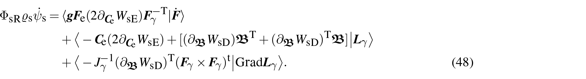
cannot be combined with any other term of the inequality (39), and, since $\hat{\mathcal{D}}$ is affine in the rates ${\stackrel{·}{\mathit{L}}}_{\gamma }$ , $\stackrel{·}{\overline{\mathrm{Grad}{\mathit{L}}_{\gamma }}}$ , $\stackrel{·}{\overline{\mathrm{Grad}{\mathit{V}}_{\mathrm{f}}}}$ , and $\stackrel{·}{\overline{{\mathit{V}}_{\mathrm{fs}}}}$ , which can be varied arbitrarily, the duality products in equations (44a) and (44b) could take on any real value and violate the non-negativity of $\hat{\mathcal{D}}$ . Thus, to prevent this occurrence, we require the partial derivatives ${\partial }_{{\mathit{L}}_{\gamma }}{\hat{\psi }}_{\mathrm{s}}$ , ${\partial }_{\mathrm{Grad}{\mathit{L}}_{\gamma }}{\hat{\psi }}_{\mathrm{s}}$ , ${\partial }_{\mathrm{Grad}{\mathit{V}}_{\mathrm{f}}}{\hat{\psi }}_{\mathrm{s}}$ , and ${\partial }_{{\mathit{V}}_{\mathrm{fs}}}{\hat{\psi }}_{\mathrm{s}}$ to vanish identically. This can be achieved by redefining the constitutive expression of ${\psi }_{\mathrm{s}}$ as a function of F , ${\mathit{F}}_{\gamma }$ , and $\mathfrak{B}$ , only. To this end, we find it convenient to introduce the solid phase Helmholtz free energy density per unit volume of ℬ, i.e., $W_{\mathrm{sR}}:={\mathrm{\Phi }}_{\mathrm{sR}}{\varrho }_{\mathrm{s}}{\psi }_{\mathrm{s}}$ , for which it holds that ${Ẇ}_{\mathrm{sR}}={\mathrm{\Phi }}_{\mathrm{sR}}{\varrho }_{\mathrm{s}}{\stackrel{·}{\psi }}_{\mathrm{s}}$ , since ${\varrho }_{\mathrm{s}}$ is assumed to be constant, while ${\mathrm{\Phi }}_{\mathrm{sR}}$ is constant by virtue of equation (7). Then, following Gurtin and Anand [38], we write

$$\begin{array}{ccc}\hfill W_{\mathrm{sR}}& ={Ŵ}_{\mathrm{sR}}\circ (\mathit{F},{\mathit{F}}_{\gamma },\mathfrak{B})={Ŵ}_{\mathrm{se}}\circ (\mathit{F},{\mathit{F}}_{\gamma })+{Ŵ}_{\mathrm{sD}}\circ \mathfrak{B},\hfill & \hfill \end{array}$$

(45)

where ${Ŵ}_{\mathrm{se}}$ is a hyperelastic free energy density of the solid phase, while ${Ŵ}_{\mathrm{sD}}$ is referred to as a “defect” free energy [38] and resolves explicitly the spatial variability of ${\mathit{F}}_{\gamma }$ within a first-order theory in the remodeling tensor (accounted for through $\mathfrak{B}$ ). In our work, this is done to account also for the influence of boundary effects on remodeling. Yet, the formalism from which we are departing adopts $\mathrm{Grad}{\mathit{F}}_{\gamma }$ to describe geometric incompatibilities that, for example, arise in metals at the scale of the lattice due to concentrated defects such as dislocations and disclinations [63,86–91].

To ensure objectivity, ${Ŵ}_{\mathrm{se}}$ depends on F and ${\mathit{F}}_{\gamma }$ through the elastic Cauchy–Green deformation tensor ${\mathit{C}}_{\mathrm{e}}={\mathit{F}}_{\mathrm{e}}^{\mathrm{T}}\mathit{g}{\mathit{F}}_{\mathrm{e}}$ . Hence, we set ${Ŵ}_{\mathrm{se}}\circ (\mathit{F},{\mathit{F}}_{\gamma })\equiv {Ŵ}_{\mathrm{sE}}\circ {\mathit{C}}_{\mathrm{e}}$ , and we reformulate ${Ŵ}_{\mathrm{sR}}$ as

$$\begin{array}{ccc}\hfill W_{\mathrm{sR}}={Ŵ}_{\mathrm{sR}}\circ (\mathit{F},{\mathit{F}}_{\gamma },\mathfrak{B})={Ŵ}_{\mathrm{sE}}\circ {\mathit{C}}_{\mathrm{e}}+{Ŵ}_{\mathrm{sD}}\circ \mathfrak{B},& \hfill & \hfill \end{array}$$

(46)

where ${Ŵ}_{\mathrm{sE}}$ and ${Ŵ}_{\mathrm{sD}}$ are to be assigned. Hence, upon introducing the short-hand notation

$$\begin{array}{ccccc}\hfill & {\partial }_{{\mathit{C}}_{\mathrm{e}}}{W}_{\mathrm{sE}}\equiv {\partial }_{{\mathit{C}}_{\mathrm{e}}}{Ŵ}_{\mathrm{sE}}\circ {\mathit{C}}_{\mathrm{e}},\hfill & \hfill & {\partial }_{\mathfrak{B}}{W}_{\mathrm{sD}}\equiv {\partial }_{\mathfrak{B}}{Ŵ}_{\mathrm{sD}}\circ \mathfrak{B},\hfill & \hfill \end{array}$$

(47)

the term ${\mathrm{\Phi }}_{\mathrm{sR}}{\varrho }_{\mathrm{s}}{\stackrel{·}{\psi }}_{\mathrm{s}}\equiv {Ẇ}_{\mathrm{sR}}$ in the inequality (39) admits the following representation [38]:

$$\begin{array}{cccc}\hfill {\mathrm{\Phi }}_{\mathrm{sR}}{\varrho }_{\mathrm{s}}{\stackrel{·}{\psi }}_{\mathrm{s}}=& ⟨\mathit{g}{\mathit{F}}_{\mathrm{e}}(2{\partial }_{{\mathit{C}}_{\mathrm{e}}}{W}_{\mathrm{sE}}){\mathit{F}}_{\gamma }^{-\mathrm{T}}|\stackrel{·}{\mathit{F}}⟩\hfill & \hfill & \hfill \\ \hfill & +⟨-{\mathit{C}}_{\mathrm{e}}(2{\partial }_{{\mathit{C}}_{\mathrm{e}}}{W}_{\mathrm{sE}})+[({\partial }_{\mathfrak{B}}{W}_{\mathrm{sD}}){\mathfrak{B}}^{\mathrm{T}}+{({\partial }_{\mathfrak{B}}{W}_{\mathrm{sD}})}^{\mathrm{T}}\mathfrak{B}]|{\mathit{L}}_{\gamma }⟩\hfill & \hfill & \hfill \\ \hfill & +⟨-J_{\gamma }^{-1}{({\partial }_{\mathfrak{B}}{W}_{\mathrm{sD}})}^{\mathrm{T}}{({\mathit{F}}_{\gamma }\times {\mathit{F}}_{\gamma })}^{\mathrm{t}}|\mathrm{Grad}{\mathit{L}}_{\gamma }⟩.\hfill & \hfill \end{array}$$

(48)

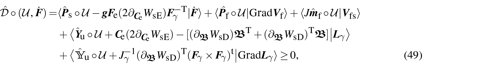
By plugging the derivative (48) into equation (39), the dissipation inequality becomes

$$\begin{array}{cccc}\hfill \hat{\mathcal{D}}\circ (\mathcal{U},\stackrel{·}{\mathit{F}})=& ⟨{\hat{\mathit{P}}}_{\mathrm{s}}\circ \mathcal{U}-\mathit{g}{\mathit{F}}_{\mathrm{e}}(2{\partial }_{{\mathit{C}}_{\mathrm{e}}}{W}_{\mathrm{sE}}){\mathit{F}}_{\gamma }^{-\mathrm{T}}|\stackrel{·}{\mathit{F}}⟩+⟨\widehat{{\mathit{P}}_{\mathrm{f}}}\circ \mathcal{U}|\mathrm{Grad}{\mathit{V}}_{\mathrm{f}}⟩+⟨J{\hat{\mathit{m}}}_{\mathrm{f}}\circ \mathcal{U}|{\mathit{V}}_{\mathrm{fs}}⟩\hfill & \hfill & \hfill \\ \hfill & +⟨{\hat{\mathit{Y}}}_{\mathrm{u}}\circ \mathcal{U}+{\mathit{C}}_{\mathrm{e}}(2{\partial }_{{\mathit{C}}_{\mathrm{e}}}{W}_{\mathrm{sE}})-[({\partial }_{\mathfrak{B}}{W}_{\mathrm{sD}}){\mathfrak{B}}^{\mathrm{T}}+{({\partial }_{\mathfrak{B}}{W}_{\mathrm{sD}})}^{\mathrm{T}}\mathfrak{B}]|{\mathit{L}}_{\gamma }⟩\hfill & \hfill & \hfill \\ \hfill & +⟨{\hat{\mathbb{Y}}}_{\mathrm{u}}\circ \mathcal{U}+J_{\gamma }^{-1}{({\partial }_{\mathfrak{B}}{W}_{\mathrm{sD}})}^{\mathrm{T}}{({\mathit{F}}_{\gamma }\times {\mathit{F}}_{\gamma })}^{\mathrm{t}}|\mathrm{Grad}{\mathit{L}}_{\gamma }⟩\ge 0,\hfill & \hfill \end{array}$$

(49)

where, with a slight abuse of notation, we have reformulated $\hat{\mathcal{D}}$ as a function of $\mathcal{U}$ and $\stackrel{·}{\mathit{F}}$ , only. However, $\hat{\mathcal{D}}$ is affine in $\stackrel{·}{\mathit{F}}$ . Hence, following the same reasoning that has conducted to equation (45), the entity dual to $\stackrel{·}{\mathit{F}}$ in the inequality (49) must vanish, and the active stress tensor ${\mathit{P}}_{\mathrm{s}}$ is represented by

$$\begin{array}{ccc}\hfill {\mathit{P}}_{\mathrm{s}}={\hat{\mathit{P}}}_{\mathrm{s}}\circ (\mathit{F},{\mathit{F}}_{\gamma })=\mathit{g}\mathit{F}{\mathit{F}}_{\gamma }^{-1}(2{\partial }_{{\mathit{C}}_{\mathrm{e}}}{W}_{\mathrm{se}}){\mathit{F}}_{\gamma }^{-\mathrm{T}}.& \hfill & \hfill \end{array}$$

(50)

Now, we particularize the hypotheses Hp. 2 and Hp. 3 by requiring each summand on the right-hand side of the inequality (49) to be non-negative independently of the other ones (the first summand satisfies trivially this requirement, since it is zero by virtue of equation (50)). Moreover, as for the fluid, for which ${\mathit{P}}_{\mathrm{f}}$ and ${\mathit{m}}_{\mathrm{f}}$ are a dissipative stress and a dissipative force density, we define the dissipative stress-like quantities

$$\begin{array}{ccc}\hfill {\mathit{Y}}_{\mathrm{ud}}={\hat{\mathit{Y}}}_{\mathrm{ud}}\circ \mathcal{U}& :={\hat{\mathit{Y}}}_{\mathrm{u}}\circ \mathcal{U}+{\mathit{C}}_{\mathrm{e}}(2{\partial }_{{\mathit{C}}_{\mathrm{e}}}{W}_{\mathrm{sE}})-[({\partial }_{\mathfrak{B}}{W}_{\mathrm{sD}}){\mathfrak{B}}^{\mathrm{T}}+{({\partial }_{\mathfrak{B}}{W}_{\mathrm{sD}})}^{\mathrm{T}}\mathfrak{B}],\hfill & \hfill \end{array}$$

(51a)

$$\begin{array}{ccc}\hfill {\mathbb{Y}}_{\mathrm{ud}}={\hat{\mathbb{Y}}}_{\mathrm{ud}}\circ \mathcal{U}& :={\hat{\mathbb{Y}}}_{\mathrm{u}}\circ \mathcal{U}+J_{\gamma }^{-1}{({\partial }_{\mathfrak{B}}{W}_{\mathrm{sD}})}^{\mathrm{T}}{({\mathit{F}}_{\gamma }\times {\mathit{F}}_{\gamma })}^{\mathrm{t}},\hfill & \hfill \end{array}$$

(51b)

and, by recalling the result (50), we write the residual dissipation inequality as

$$\begin{array}{ccc}\hfill \hat{\mathcal{D}}\circ \mathcal{U}=& ⟨{\hat{\mathit{P}}}_{\mathrm{f}}\circ \mathcal{U}|\mathrm{Grad}{\mathit{V}}_{\mathrm{f}}⟩+⟨J{\hat{\mathit{m}}}_{\mathrm{f}}\circ \mathcal{U}|{\mathit{V}}_{\mathrm{fs}}⟩+⟨{\hat{\mathit{Y}}}_{\mathrm{ud}}\circ \mathcal{U}|{\mathit{L}}_{\gamma }⟩+⟨{\hat{\mathbb{Y}}}_{\mathrm{ud}}\circ \mathcal{U}|\mathrm{Grad}{\mathit{L}}_{\gamma }⟩\ge 0.\hfill & \hfill \end{array}$$

(52)

In the inequality (52), we split $\mathcal{U}$ into the two sub-collections of variables $\mathcal{E}:=(\mathit{F},{\mathit{F}}_{\gamma },\mathfrak{B})$ and $\mathcal{R}:=({\mathit{L}}_{\gamma },\mathrm{Grad}{\mathit{L}}_{\gamma },\mathrm{Grad}{\mathit{V}}_{\mathrm{f}},{\mathit{V}}_{\mathrm{fs}})$ , with the latter comprising all the rates considered in the model, and we require $\hat{\mathcal{D}}\circ \mathcal{U}\equiv \hat{\mathcal{D}}\circ (\mathcal{E};\mathcal{R})$ to be non-negative for all $\mathcal{E}$ and $\mathcal{R}$ , null for $\mathcal{R}=0$ independently of $\mathcal{E}$ (i.e., $\hat{\mathcal{D}}\circ (\mathcal{E};0)=0$ uniformly with respect to $\mathcal{E}$ ), continuous and differentiable in $\mathcal{E}$ , and at least continuous in $\mathcal{R}$ . The continuity of $\hat{\mathcal{D}}$ in $\mathcal{R}$ is needed to ensure that $\hat{\mathcal{D}}\circ (\mathcal{E};\mathcal{R})$ tends to zero for indefinitely small rates $\mathcal{R}$ . We refer to the work by Cermelli et al. [85] for the reasoning reported so far.

In the following, we further assume $\hat{\mathcal{D}}$ to be quadratic in the rates $\mathcal{R}$ , as specified by the law

$$\begin{array}{cccc}\hfill \hat{\mathcal{D}}\circ (\mathcal{E};\mathcal{R})=& {\mathrm{\Phi }}_{\mathrm{fR}}⟨\mathbb{V}:\mathrm{Grad}{\mathit{V}}_{\mathrm{f}}|\mathrm{Grad}{\mathit{V}}_{\mathrm{f}}⟩+{\mathrm{\Phi }}_{\mathrm{fR}}⟨\mathit{r}{\mathit{V}}_{\mathrm{fs}}|{\mathit{V}}_{\mathrm{fs}}⟩\hfill & \hfill & \hfill \\ \hfill & +{\mathrm{\Phi }}_{\mathrm{sR}}{S}_{\mathrm{y}}\parallel {\mathit{L}}_{\gamma }{\mathrm{\parallel }}^2+{\mathrm{\Phi }}_{\mathrm{sR}}{S}_{\mathrm{y}}{\ell }^2\parallel \mathrm{Grad}{\mathit{L}}_{\gamma }{\mathrm{\parallel }}^2\ge 0,\hfill & \hfill \end{array}$$

(53)

where ${\mathrm{\Phi }}_{\mathrm{fR}}=J-{\mathrm{\Phi }}_{\mathrm{sR}}\ge 0$ depends on F through J; $\mathbb{V}:=\hat{\mathbb{V}}\circ \mathcal{E}$ and $\mathit{r}=\hat{\mathit{r}}\circ \mathcal{E}$ are a fourth-order and a second-order tensor field, both positive semi-definite; $S_{\mathrm{y}}>0$ and $\ell >0$ are constants representing a characteristic mechanical stress of the solid phase and the characteristic length of ${\mathit{L}}_{\gamma }$ , respectively [38]; the squared norms $\parallel {\mathit{L}}_{\gamma }{\mathrm{\parallel }}^2$ and $\parallel \mathrm{Grad}{\mathit{L}}_{\gamma }{\mathrm{\parallel }}^2$ are defined by

$$\begin{array}{ccc}\hfill \parallel {\mathit{L}}_{\gamma }{\mathrm{\parallel }}^2& =⟨{\mathit{L}}_{\gamma }^{\ast }|{\mathit{L}}_{\gamma }⟩=G_{\mathrm{AB}}{[{\mathit{L}}_{\gamma }{]}^B}_C{G}^{\mathrm{CD}}{[{\mathit{L}}_{\gamma }{]}^A}_D=\mathrm{tr}[{\mathit{L}}_{\gamma }^{\ast \mathrm{T}}{\mathit{L}}_{\gamma }],\hfill & \hfill \end{array}$$

(54a)

$$\begin{array}{cc}\hfill \parallel \mathrm{Grad}{\mathit{L}}_{\gamma }{\mathrm{\parallel }}^2& =⟨{(\mathrm{Grad}{\mathit{L}}_{\gamma })}^{\ast }|\mathrm{Grad}{\mathit{L}}_{\gamma }⟩=G_{\mathrm{AH}}{[\mathrm{Grad}{\mathit{L}}_{\gamma }{]}^H}_{\mathrm{MN}}{G}^{\mathrm{MB}}{G}^{\mathrm{NC}}{[\mathrm{Grad}{\mathit{L}}_{\gamma }{]}^A}_{\mathrm{BC}},\hfill \end{array}$$

(54b)

where ${\mathit{L}}_{\gamma }^{\ast }:=\mathit{G}{\mathit{L}}_{\gamma }{\mathit{G}}^{-1}$ and ${(\mathrm{Grad}{\mathit{L}}_{\gamma })}^{\ast }$ are the tensor fields dual to ${\mathit{L}}_{\gamma }$ and $\mathrm{Grad}{\mathit{L}}_{\gamma }$ . The components of ${(\mathrm{Grad}{\mathit{L}}_{\gamma })}^{\ast }$ are given by the product of the first four factors on the right-hand side of equation (54b).

Since in this work we need the stronger condition that $\hat{\mathcal{D}}\circ (\mathcal{E};\mathcal{R})$ be zero if, and only if, all the rates are null, i.e., $\mathcal{R}=0$ , we consider only positive definite tensor-valued functions $\hat{\mathbb{V}}\circ \mathcal{E}$ and $\hat{\mathit{r}}\circ \mathcal{E}$ . Analogously, although ${\mathrm{\Phi }}_{\mathrm{fR}}$ is non-negative in general, we assume ${\mathrm{\Phi }}_{\mathrm{fR}}>0$ , meaning no compaction. Moreover, since the duality products in equation (53) symmetrize $\mathbb{V}$ and r , we shall assume from here on that $\mathbb{V}$ possesses major symmetry and that r is symmetric. Hence, in components, we have ${{{\mathbb{V}}_a}^A}_{b^B}={{{\mathbb{V}}_a}^B}_{b^A}$ and $r_{\mathrm{ab}}=r_{\mathrm{ba}}$ .

Starting from the inequality (53), we retrieve the Darcy–Brinkman model of the flow and a strain-gradient theory of remodeling à la Gurtin and Anand [38] by invoking the Principle of Maximum Dissipation (see, e.g., Hackl and Fischer [92]).

4.3. Elastic energy and “defect” energy

To supply constitutive expressions for ${\mathit{P}}_{\mathrm{s}}$ , ${\mathit{Y}}_{\mathrm{u}}$ , and ${\mathbb{Y}}_{\mathrm{u}}$ , we prescribe a Neo-Hookean strain energy density for the hyperelastic behavior of the solid phase and, following Gurtin and Anand [38], a “defect” energy density quadratic in the Burgers tensor, i.e.,

$$\begin{array}{ccc}\hfill & {Ŵ}_{\mathrm{sE}}\circ {\mathit{C}}_{\mathrm{e}}=\frac{1}{2}{\mathrm{\Phi }}_{\mathrm{sR}}{\mu }_{\mathrm{s}}[\mathrm{tr}({\mathit{G}}^{-1}{\mathit{C}}_{\mathrm{e}})-3]-{\mathrm{\Phi }}_{\mathrm{sR}}{\mu }_{\mathrm{s}}\log J_{\mathrm{e}}+\frac{1}{2}{\mathrm{\Phi }}_{\mathrm{sR}}{\lambda }_{\mathrm{s}}{[\log J_{\mathrm{e}}]}^2,\hfill & \hfill \end{array}$$

(55a)

$$\begin{array}{ccc}\hfill & {Ŵ}_{\mathrm{sD}}\circ \mathfrak{B}=\frac{1}{2}{\mathrm{\Phi }}_{\mathrm{sR}}{\mu }_{\mathrm{s}}{L}^2\parallel \mathfrak{B}{\mathrm{\parallel }}^2,\mathrm{with}\parallel \mathfrak{B}{\mathrm{\parallel }}^2=⟨{\mathfrak{B}}^{\ast }|\mathfrak{B}⟩=\mathrm{tr}({\mathfrak{B}}^{\ast \mathrm{T}}\mathfrak{B}),\hfill & \hfill \end{array}$$

(55b)

where ${\mathfrak{B}}^{\ast }:=\mathit{G}\mathfrak{B}\mathit{G}$ is the dual of the Burgers tensor, ${\mu }_{\mathrm{s}}$ and ${\lambda }_{\mathrm{s}}$ are the first and the second Lamé parameters, and L is a phenomenological length scale that, as remarked by Gurtin and Anand [38], should be determined experimentally. Then, with $J_{\gamma }=1$ , the relations (50), (51a), and (51b) take on the form

$$\begin{array}{ccc}\hfill & {\mathit{P}}_{\mathrm{s}}={\hat{\mathit{P}}}_{\mathrm{s}}\circ (\mathit{F},{\mathit{F}}_{\gamma })={\mathrm{\Phi }}_{\mathrm{sR}}{\mu }_{\mathrm{s}}[\mathit{g}\mathit{F}{\mathit{B}}_{\gamma }-{\mathit{F}}^{-\mathrm{T}}]+({\mathrm{\Phi }}_{\mathrm{sR}}{\lambda }_{\mathrm{s}}\log J){\mathit{F}}^{-\mathrm{T}},\hfill & \hfill \end{array}$$

(56a)

$$\begin{array}{ccc}\hfill & {\mathit{Y}}_{\mathrm{u}}={\hat{\mathit{Y}}}_{\mathrm{u}}\circ \mathcal{U}={\hat{\mathit{Y}}}_{\mathrm{ud}}\circ \mathcal{U}-{\mathit{F}}_{\gamma }^{-\mathrm{T}}[{\mathit{F}}^{\mathrm{T}}{\mathit{P}}_{\mathrm{s}}]{\mathit{F}}_{\gamma }^{\mathrm{T}}+{\mathrm{\Phi }}_{\mathrm{sR}}{\mu }_{\mathrm{s}}{L}^2[{\mathfrak{B}}^{\ast }{\mathfrak{B}}^{\mathrm{T}}+{\mathfrak{B}}^{\ast \mathrm{T}}\mathfrak{B}],\hfill & \hfill \end{array}$$

(56b)

$$\begin{array}{ccc}\hfill & {\mathbb{Y}}_{\mathrm{u}}={\hat{\mathbb{Y}}}_{\mathrm{u}}\circ \mathcal{U}={\hat{\mathbb{Y}}}_{\mathrm{ud}}\circ \mathcal{U}-{\mathrm{\Phi }}_{\mathrm{sR}}{\mu }_{\mathrm{s}}{L}^2{\mathfrak{B}}^{\ast \mathrm{T}}{({\mathit{F}}_{\gamma }\times {\mathit{F}}_{\gamma })}^{\mathrm{t}},\hfill & \hfill \end{array}$$

(56c)

with ${\mathit{F}}^{\mathrm{T}}{\mathit{P}}_{\mathrm{s}}$ being the Mandel stress tensor of the solid phase, associated with the reference placement.

4.4. Constitutive relations for the generalized internal forces that drive remodeling

Applying the Principle of Maximum Dissipation [92] to the summands of the dissipation inequality (53) associated with the remodeling yields

$$\begin{array}{ccc}\hfill & {\mathit{Y}}_{\mathrm{ud}}={\hat{\mathit{Y}}}_{\mathrm{ud}}\circ {\mathit{L}}_{\gamma }:=\frac{1}{2}(\frac{\partial \hat{\mathcal{D}}}{\partial {\mathit{L}}_{\gamma }}\circ (\mathcal{E};\mathcal{R}))={\mathrm{\Phi }}_{\mathrm{sR}}{S}_{\mathrm{y}}{\mathit{L}}_{\gamma }^{\ast },\hfill & \hfill \end{array}$$

(57a)

$$\begin{array}{ccc}\hfill & {\mathbb{Y}}_{\mathrm{ud}}={\hat{\mathbb{Y}}}_{\mathrm{ud}}\circ \mathrm{Grad}{\mathit{L}}_{\gamma }:=\frac{1}{2}(\frac{\partial \hat{\mathcal{D}}}{\partial \mathrm{Grad}{\mathit{L}}_{\gamma }}\circ (\mathcal{E};\mathcal{R}))={\mathrm{\Phi }}_{\mathrm{sR}}{S}_{\mathrm{y}}{\ell }^2{(\mathrm{Grad}{\mathit{L}}_{\gamma })}^{\ast }.\hfill & \hfill \end{array}$$

(57b)

The relations (57a) and (57b) are a rewriting, in covariant formalism, and up to the rescaling of $S_{\mathrm{y}}$ through ${\mathrm{\Phi }}_{\mathrm{sR}}$ and the choice of some model parameters, of the constitutive laws proposed in equation (6.17) of the work by Gurtin and Anand [38]. Indeed, in Cartesian coordinates, they read ${\mathit{Y}}_{\mathrm{ud}}={\mathrm{\Phi }}_{\mathrm{sR}}{S}_{\mathrm{y}}{\mathit{L}}_{\gamma }$ and ${\mathbb{Y}}_{\mathrm{ud}}={\mathrm{\Phi }}_{\mathrm{sR}}{S}_{\mathrm{y}}{\ell }^2\mathrm{Grad}{\mathit{L}}_{\gamma }$ , which are identical to the laws reported in the work by Gurtin and Anand [38] upon taking an identically null “hardening (softening) function” and unitary “rate-sensitivity parameter” [38]. Moreover, if the constraint (10b) is enforced explicitly, as done by Gurtin and Anand [38], then ${\mathit{L}}_{\gamma }$ and $\mathrm{Grad}{\mathit{L}}_{\gamma }$ can be substituted with ${\mathit{D}}_{\gamma }$ and $\mathrm{Grad}{\mathit{D}}_{\gamma }$ in the relations (57a) and (57b).

Within their theory of strain-gradient plasticity, Gurtin and Anand [38] call $S_{\mathrm{y}}>0$ “coarse grain yield strength” of the material, and introduce the length scale $\ell >0$ to characterize the dissipation associated with the spatial inhomogeneity of ${\mathit{L}}_{\gamma }$ .

In our framework, we neglect any hardening or softening effects as well as any nonlinear relations similar to the “nearly rate-independent behavior” accounted for by Gurtin and Anand [38]. Indeed, the functional forms (57a) and (57b) are linear in ${\mathit{L}}_{\gamma }$ and $\mathrm{Grad}{\mathit{L}}_{\gamma }$ , respectively, and have been obtained by requiring $\hat{\mathcal{D}}$ to be quadratic in each of these variables. Hence, they may fail to capture some particular physical aspects of remodeling. However, a more general picture can be obtained by hypothesizing ${\mathit{Y}}_{\mathrm{ud}}$ and ${\mathbb{Y}}_{\mathrm{ud}}$ to be nonlinear in ${\mathit{L}}_{\gamma }$ and $\mathrm{Grad}{\mathit{L}}_{\gamma }$ [38], and showing that the resulting dissipation is non-negative.

Substituting the relations (57a) and (57b) into the expressions (56b) and (56c) for ${\mathit{Y}}_{\mathrm{u}}$ and ${\mathbb{Y}}_{\mathrm{u}}$ , and defining the apparent material parameters ${\overline{S}}_{\mathrm{y}}:={\mathrm{\Phi }}_{\mathrm{sR}}{S}_{\mathrm{y}}$ , ${\overline{\mu }}_{\mathrm{s}}:={\mathrm{\Phi }}_{\mathrm{sR}}{\mu }_{\mathrm{s}}$ and ${\overline{\lambda }}_{\mathrm{s}}={\mathrm{\Phi }}_{\mathrm{sR}}{\lambda }_{\mathrm{s}}$ lead to

$$\begin{array}{ccc}\hfill {\mathit{Y}}_{\mathrm{u}}& ={\hat{\mathit{Y}}}_{\mathrm{u}}\circ (\mathcal{E};{\mathit{L}}_{\gamma })={\overline{S}}_{\mathrm{y}}{\mathit{L}}_{\gamma }^{\ast }-{\mathit{F}}_{\gamma }^{-\mathrm{T}}[{\mathit{F}}^{\mathrm{T}}{\mathit{P}}_{\mathrm{s}}]{\mathit{F}}_{\gamma }^{\mathrm{T}}+{\overline{\mu }}_{\mathrm{s}}{L}^2[{\mathfrak{B}}^{\ast }{\mathfrak{B}}^{\mathrm{T}}+{\mathfrak{B}}^{\ast \mathrm{T}}\mathfrak{B}],\hfill & \hfill \end{array}$$

(58a)

$$\begin{array}{ccc}\hfill {\mathbb{Y}}_{\mathrm{u}}& ={\hat{\mathbb{Y}}}_{\mathrm{u}}\circ (\mathcal{E};\mathrm{Grad}{\mathit{L}}_{\gamma })={\overline{S}}_{\mathrm{y}}{\ell }^2{(\mathrm{Grad}{\mathit{L}}_{\gamma })}^{\ast }-{\overline{\mu }}_{\mathrm{s}}{L}^2{\mathfrak{B}}^{\ast \mathrm{T}}{({\mathit{F}}_{\gamma }\times {\mathit{F}}_{\gamma })}^{\mathrm{t}},\hfill & \hfill \end{array}$$

(58b)

where we have set $J_{\gamma }=1$ and, with a slight abuse of notation, we have retained the sole dependence on ${\mathit{L}}_{\gamma }$ and $\mathrm{Grad}{\mathit{L}}_{\gamma }$ . Finally, by using the results (58a) and (58b), equation (33e) becomes

$$\begin{array}{cccc}\hfill & {\overline{S}}_{\mathrm{y}}{\mathit{L}}_{\gamma }^{\ast }-{\mathit{F}}_{\gamma }^{-\mathrm{T}}[{\mathit{F}}^{\mathrm{T}}{\mathit{P}}_{\mathrm{s}}]{\mathit{F}}_{\gamma }^{\mathrm{T}}+{\overline{\mu }}_{\mathrm{s}}{L}^2[{\mathfrak{B}}^{\ast }{\mathfrak{B}}^{\mathrm{T}}+{\mathfrak{B}}^{\ast \mathrm{T}}\mathfrak{B}]+\eta {\mathit{I}}^{\mathrm{T}}+\mathit{G}(\mathrm{Skew}\mathit{{\rm Y}})\hfill & \hfill & \hfill \\ \hfill & -\mathrm{Div}\{{\overline{S}}_{\mathrm{y}}{\ell }^2{(\mathrm{Grad}{\mathit{L}}_{\gamma })}^{\ast }-{\overline{\mu }}_{\mathrm{s}}{L}^2{\mathfrak{B}}^{\ast \mathrm{T}}{({\mathit{F}}_{\gamma }\times {\mathit{F}}_{\gamma })}^{\mathrm{t}}\}-\mathit{Z}=\mathit{O}.\hfill & \hfill \end{array}$$

(59)

The partial differential equation (59) and the constraints (33h) and (33i) rephrase, for remodeling, one of the main results of the theory of strain-gradient plasticity of Gurtin and Anand [38], formulated for ${\mathit{D}}_{\gamma }$ . In our derivation, we develop the model for ${\mathit{L}}_{\gamma }$ and enforce the constraints on it via the Lagrange multiplier technique (see Section 2.3), which generates the reaction force $\eta {\mathit{I}}^{\mathrm{T}}+\mathit{G}(\mathrm{Skew}\mathit{{\rm Y}})$ in equation (59). This can be eliminated by projecting equation (59) onto the space of deviatoric and symmetric second-order tensor fields, as shown in equation (34c), thereby retrieving Gurtin and Anand’s strain-gradient “micro-force balance” [38]. Moreover, in our work, this result is framed within the context of solid-fluid mixtures. However, the coupling with the fluid is indirect and occurs through the influence that the fields associated with the fluid (i.e., pressure p and velocity field ${\mathit{V}}_{\mathrm{f}}$ ) exert on F (and, thus, on ${\mathit{P}}_{\mathrm{s}}$ ). Another generalization is the presence of Z , unaccounted for in the work by Gurtin and Anand [38], but relevant in the certain biological contexts, as is the case for growth [23,83].

4.5. Darcy–Brinkman model for the flow of the interstitial fluid

The Darcy–Brinkman model [41] of the flow accounts for two independent types of dissipation, both related to the fluid (see Hp. 3). One is intrinsic to the fluid and hypothesizes a macroscopically viscous behavior, described by the dissipative stress tensor ${\mathit{P}}_{\mathrm{f}}$ . The other one, instead, stems from the dissipative character of the interactions between the solid and the fluid, described by ${\mathit{m}}_{\mathrm{f}}$ . By applying the formulation of the Principle of Maximum Dissipation presented by Hackl and Fischer [92] to the terms in the dissipation inequality (53) associated with the fluid flow, we find

$$\begin{array}{ccc}\hfill & {\mathit{P}}_{\mathrm{f}}={\hat{\mathit{P}}}_{\mathrm{f}}\circ (\mathcal{E};\mathcal{R}):=\frac{1}{2}(\frac{\partial \hat{\mathcal{D}}}{\partial \mathrm{Grad}{\mathit{V}}_{\mathrm{f}}}\circ (\mathcal{E};\mathcal{R}))={\mathrm{\Phi }}_{\mathrm{fR}}[\hat{\mathbb{V}}\circ \mathcal{E}]:\mathrm{Grad}{\mathit{V}}_{\mathrm{f}},\hfill & \hfill \end{array}$$

(60a)

$$\begin{array}{ccc}\hfill & J{\mathit{m}}_{\mathrm{f}}=J[{\hat{\mathit{m}}}_{\mathrm{f}}\circ (\mathcal{E};\mathcal{R})]:=\frac{1}{2}(\frac{\partial \hat{\mathcal{D}}}{\partial {\mathit{V}}_{\mathrm{fs}}}\circ (\mathcal{E};\mathcal{R}))={\mathrm{\Phi }}_{\mathrm{fR}}[\hat{\mathit{r}}\circ \mathcal{E}]{\mathit{V}}_{\mathrm{fs}},\hfill & \hfill \end{array}$$

(60b)

where $\mathbb{V}=\hat{\mathbb{V}}\circ \mathcal{E}$ is a fourth-order tensor field of generalized Brinkman viscosities and $\mathit{r}=\hat{\mathit{r}}\circ \mathcal{E}$ is the (spatial) resistivity tensor field of the porous medium (as specified above, $\mathbb{V}$ enjoys major symmetry and r is symmetric). Since r is positive definite, it is invertible, and we identify its inverse with the expression

$$\begin{array}{ccc}\hfill & {\mathit{r}}^{-1}={\varphi }_{\mathrm{fR}}^{-1}\mathit{k},\hfill & \hfill \end{array}$$

(61)

where k is the tensor field of the hydraulic conductivity of the medium (i.e., the permeability tensor field divided by the fluid dynamic viscosity). The tensor field k is symmetric and positive definite, too. We prescribe it to be a function of F only, and, since we are modeling biological tissues, we express it as suggested by Holmes and Mow [1], i.e.,

$$\begin{array}{ccc}\hfill \mathit{k}=\hat{\mathit{k}}\circ \mathit{F}=k_0[\frac{J-{\mathrm{\Phi }}_{\mathrm{sR}}}{1-{\mathrm{\Phi }}_{\mathrm{sR}}}{]}^{\kappa }\exp (\frac{1}{2}{m}_0[J^2-1]){\mathit{g}}^{-1},& \hfill & \hfill \end{array}$$

(62)

where $k_0$ , κ, and $m_0$ are positive material parameters (see Table 1).

Table 1.

Values of the material parameters used for the numerical simulations.

Parameter	Symbol	Numerical value	Unit of measure	Reference
Initial radius	R	$5.0$	$\mathrm{mm}$	-
Initial height	H	$10.0$	$\mathrm{mm}$	-
Referential solidity	${\mathrm{\Phi }}_{\mathrm{sR}}$	$0.6$	-	-
Referential hydraulic conductivity	$k_0$	$2.557\cdot 10^{-2}$	${\mathrm{mm}}^4∕(\mathrm{N}\cdot \mathrm{s})$	-
Material parameter	$m_0$	0.0848	-	Holmes [96]
Material parameter	κ	4.6380	-	Holmes [96]
First Lamé’s constant	${\lambda }_{\mathrm{s}}$	$1.3\cdot 10^4$	$\mathrm{Pa}$	-
Second Lamé’s constant	${\mu }_{\mathrm{s}}$	$2.0\cdot 10^4$	$\mathrm{Pa}$	-
Coarse grain yield strength	$S_{\mathrm{y}}$	$1.0\cdot 10^3$	$\mathrm{Pa}\cdot \mathrm{s}$	-
Dissipative length [38]	ℓ	$1.0$	$\mathrm{mm}$	-
Energetic length [38]	L	$1.0$	$\mathrm{mm}$	-
Volumetric fluid viscosity coefficient	$\mathfrak{a}$	$0.0^a$	$\mathrm{Pa}\cdot \mathrm{s}$	-
Shear fluid viscosity coefficient	$\mathfrak{b}$	$1.0\cdot 10^{-3}$	$\mathrm{Pa}\cdot \mathrm{s}$	-
Prescribed displacement	$f_{\max }$	2.0	$\mathrm{mm}$	-
Loading time	$t_{\mathrm{r}}$	10.0	$\mathrm{s}$	-
End time	$t_{\mathrm{e}}$	20.0	$\mathrm{s}$	-

a

Note that, in some simulations, the value $\mathfrak{a}=100.0\mathrm{Pa}\cdot \mathrm{s}$ is assigned to obtain the Brinkman viscosity $\mathfrak{a}∕3$ .

To assign $\mathbb{V}=\hat{\mathbb{V}}\circ \mathcal{E}$ , we start from the constitutive expression of the Cauchy stress tensor of the fluid phase, i.e., ${\mathit{\sigma }}_{\mathrm{f}}=J^{-1}{\mathit{P}}_{\mathrm{f}}{\mathit{F}}^{\mathrm{T}}$ , which, under the hypothesis of Newtonian-like behavior, can be written as

$$\begin{array}{ccc}\hfill & {\mathit{\sigma }}_{\mathrm{f}}=\frac{1}{3}{\varphi }_{\mathrm{f}}\mathfrak{a}(\mathrm{div}{\mathit{v}}_{\mathrm{f}}){\mathit{ı}}^{\mathrm{T}}+2{\varphi }_{\mathrm{f}}\mathfrak{b}\mathrm{sym}(\mathit{g}\mathrm{grad}{\mathit{v}}_{\mathrm{f}}){\mathit{g}}^{-1},\hfill & \hfill \end{array}$$

(63)

where $\mathfrak{a}∕3$ and $\mathfrak{b}$ are the Brinkman viscosity coefficients, fulfilling the inequalities $\mathfrak{a}+2\mathfrak{b}>0$ and $\mathfrak{b}>0$ , and $\mathit{ı}:T\mathcal{S}\to T\mathcal{S}$ is the spatial identity tensor field (note that, for simplicity, in these calculations we are omitting the composition of the involved fields with the maps χ and $\mathcal{T}$ ). Then, by computing ${\mathit{P}}_{\mathrm{f}}=J{\mathit{\sigma }}_{\mathrm{f}}{\mathit{F}}^{-\mathrm{T}}$ , we obtain the expression (60a) with

$$\begin{array}{ccc}\hfill & \mathbb{V}=\hat{\mathbb{V}}\circ \mathit{F}:=\frac{1}{3}\mathfrak{a}{\mathit{F}}^{-\mathrm{T}}\otimes {\mathit{F}}^{-\mathrm{T}}+\mathfrak{b}(\mathit{g}\underline{\otimes }{\mathit{C}}^{-1}+{\mathit{F}}^{-\mathrm{T}}\overline{\otimes }{\mathit{F}}^{-1}),\hfill & \hfill \end{array}$$

(64a)

$$\begin{array}{cc}\hfill & \mathbb{V}{a}^A{b}^B=\frac{1}{3}\mathfrak{a}{[{\mathit{F}}^{-\mathrm{T}}{]}_a}^A{[{\mathit{F}}^{-\mathrm{T}}{]}_b}^B+\mathfrak{b}(g_{\mathrm{ab}}{[{\mathit{C}}^{-1}]}^{\mathrm{AB}}+{[{\mathit{F}}^{-\mathrm{T}}{]}_a}^B{[{\mathit{F}}^{-1}{]}^A}_b),\hfill \end{array}$$

(64b)

where $\hat{\mathbb{V}}$ has been redefined as a function of F alone, and the notation introduced by Curnier et al. [93] has been adopted for the tensor products $\underline{\otimes }$ and $\overline{\mathrm{\otimes }}$ . Note that, by virtue of equation (64a), and recalling that ${\mathrm{\Phi }}_{\mathrm{fR}}=J-{\mathrm{\Phi }}_{\mathrm{sR}}$ , the constitutive representation of ${\mathit{P}}_{\mathrm{f}}$ can be reformulated as

$$\begin{array}{ccc}\hfill & {\mathit{P}}_{\mathrm{f}}={\hat{\mathit{P}}}_{\mathrm{f}}\circ (\mathit{F},\mathrm{Grad}{\mathit{V}}_{\mathrm{f}})=(J-{\mathrm{\Phi }}_{\mathrm{sR}})(\hat{\mathbb{V}}\circ \mathit{F}):\mathrm{Grad}{\mathit{V}}_{\mathrm{f}}.\hfill & \hfill \end{array}$$

(65)

The quantity $\frac{1}{3}\mathfrak{a}$ corresponds to the so-called “second viscosity”, also known as “bulk viscosity” or “volume viscosity”, that, within the monophasic framework, features in the compressible Navier–Stokes equation. However, in spite of this formal correspondence, $\frac{1}{3}\mathfrak{a}$ is physically distinct from the second viscosity of a compressible fluid (see Remark 2 below). From here on, we refer to $\frac{1}{3}\mathfrak{a}$ and $\mathfrak{b}$ as Brinkman second viscosity and Brinkman dynamic viscosity, respectively. Often, $\mathfrak{b}$ is also referred to as effective viscosity and is assumed to be different from the “true” viscosity of the fluid. Bear and Bachmat [94] express $\mathfrak{b}$ as proportional to the fluid true shear viscosity, with the proportionality factor being the ratio between the (scalar) tortuosity and the porosity of the porous medium in which the flow takes place.

Differently from the Darcian model, in which the Cauchy stress tensor of the fluid phase is the hydrostatic term $-{\varphi }_{\mathrm{f}}p{\mathit{ı}}^{\mathrm{T}}$ , the Darcy–Brinkman model distinguishes the pressure contribution due to the Lagrange multiplier p from the viscous one. In other words, the fluid pressure is given by

$$\begin{array}{ccc}\hfill & p_{\mathrm{f}}:=-\frac{1}{3}\mathrm{tr}(-{\varphi }_{\mathrm{f}}p{\mathit{ı}}^{\mathrm{T}}+{\mathit{\sigma }}_{\mathrm{f}})={\varphi }_{\mathrm{f}}p-{\varphi }_{\mathrm{f}}\frac{\mathfrak{a}+2\mathfrak{b}}{3}\mathrm{div}{\mathit{v}}_{\mathrm{f}}.\hfill & \hfill \end{array}$$

(66)

Although the fluid phase is assumed to be incompressible, the divergence of ${\mathit{v}}_{\mathrm{f}}$ is not zero. Rather, the hypothesis of incompressibility, enforced also for the solid phase, is expressed by equation (6), and the model of flow features the Brinkman bulk viscosity $(\mathfrak{a}+2\mathfrak{b})∕3$ . However, if the velocity field of the solid phase is null and the volumetric fraction of the fluid phase is constant in space, equation (6) reduces to $\mathrm{div}{\mathit{v}}_{\mathrm{f}}=0$ and, thus, ${\mathit{\sigma }}_{\mathrm{f}}$ features only the contribution due to the Brinkman dynamic viscosity $\mathfrak{b}$ . This approximation is often used in hydro-geological problems based on the Darcy–Brinkman flow model.

By substituting the relations (60a) and (60b) into (33b), and using (61), we obtain

$$\begin{array}{ccc}\hfill & \mathrm{Div}({\mathrm{\Phi }}_{\mathrm{fR}}\mathbb{V}:\mathrm{Grad}{\mathit{V}}_{\mathrm{f}})-{\mathrm{\Phi }}_{\mathrm{fR}}[({\mathit{F}}^{-\mathrm{T}}\mathrm{Grad}p-{\varrho }_{\mathrm{f}}\mathit{f})+{\varphi }_{\mathrm{fR}}{\mathit{k}}^{-1}({\mathit{V}}_{\mathrm{f}}-{\mathit{V}}_{\mathrm{s}})]=\mathbf{0}.\hfill & \hfill \end{array}$$

(67)

Equation (67) is a partial differential equation for the fluid velocity field ${\mathit{V}}_{\mathrm{f}}$ , coupled with the pressure field p and with the velocity field ${\mathit{V}}_{\mathrm{s}}$ and deformation of the solid phase. Since $\mathbb{V}$ is positive definite and ${\mathrm{\Phi }}_{\mathrm{fR}}>0$ , equation (67) is elliptic in ${\mathit{V}}_{\mathrm{f}}$ .

Remark 2. (Comparison with the stress tensor of a compressible fluid in the monophasic framework). Within the monophasic framework, the dissipative part of the stress tensor of a compressible fluid features the volumetric contribution $\zeta (\mathrm{div}\mathit{v}){\mathit{ı}}^{\mathrm{T}}$ , in which v is the velocity field of the fluid and ζ is a positive quantity termed volume viscosity coefficient (in the Newtonian case, ζ is independent of the velocity gradient). Yet, ζ is not necessarily equal to $(\mathfrak{a}+2\mathfrak{b})∕3$ . There are two main reasons for this. First, ζ pertains to the description of a compressible fluid in the monophasic framework, whereas the bulk Brinkman viscosity $(\mathfrak{a}+2\mathfrak{b})∕3$ is defined also for an incompressible fluid phase in a fluid-solid biphasic mixture. Second, the Brinkman viscosities need not be equal to the viscosities that the same fluid would have if it were considered alone, i.e., decontextualized from the framework of mixture theory [41], although the two types of viscosities take values that become increasingly closer to each other for relatively small volumetric fractions of the solid phase.

5. Boundary-value problem, “effective” weak form, and numerical results

By substituting the constitutive relations (50), (58a), (58b), (60a), and (60b) into the system (33a)–(33i), and applying Dirichlet boundary conditions and initial conditions, we state an initial- and boundary-value problem (IBVP) for χ, ${\mathit{F}}_{\gamma }$ , ${\mathit{V}}_{\mathrm{f}}$ and p. However, the boundary condition (33f), i.e.,

$$\begin{array}{ccccc}\hfill {\mathbb{Y}}_{\mathrm{u}}\mathit{N}& ={\overline{S}}_{\mathrm{y}}{\ell }^2{(\mathrm{Grad}{\mathit{L}}_{\gamma })}^{\ast }\mathit{N}-{\overline{\mu }}_{\mathrm{s}}{L}^2{\mathfrak{B}}^{\ast \mathrm{T}}{({\mathit{F}}_{\gamma }\times {\mathit{F}}_{\gamma })}^{\mathrm{t}}\mathit{N}=\mathit{O},\hfill & \hfill & \mathrm{on}\partial ℬ,\hfill & \hfill \end{array}$$

(68)

does not have the expression of a classical Neumann boundary condition in ${\mathit{F}}_{\gamma }$ , since it involves also ${\stackrel{·}{\mathit{F}}}_{\gamma }$ , $\mathrm{Grad}{\stackrel{·}{\mathit{F}}}_{\gamma }$ , and $\mathrm{Curl}{\mathit{F}}_{\gamma }$ , as can be recognized by writing it explicitly.

To overcome this difficulty, we reformulate the IBVP by regarding ${\mathit{L}}_{\gamma }$ as a primary unknown, rather than as a derived quantity, and we regard the relation ${\stackrel{·}{\mathit{F}}}_{\gamma }={\mathit{L}}_{\gamma }{\mathit{F}}_{\gamma }$ as the additional equation for determining ${\mathit{F}}_{\gamma }$ . By doing so, equation (59) can be recast in the form of a (linear) modified Helmholtz equation [95] in ${\mathit{L}}_{\gamma }$ , with a right-hand side that is highly nonlinear in F and ${\mathit{F}}_{\gamma }$ , and equation (68) can be interpreted as a linear, nonhomogeneous, Neumann boundary condition for ${\mathit{L}}_{\gamma }$ , in which the non-homogeneity term depends on ${\mathit{F}}_{\gamma }$ through ${\mathit{F}}_{\gamma }\times {\mathit{F}}_{\gamma }$ and the Burgers tensor $\mathfrak{B}$ . Moreover, the constraints (33h) and (33i) become algebraic equations for ${\mathit{L}}_{\gamma }$ . This fact permits us to resolve them explicitly and, thus, to replace the nine unknown components of ${\mathit{L}}_{\gamma }$ with the five unknown components of the symmetric and deviatoric tensor ${\tilde{\mathit{D}}}_{\gamma }$ , which satisfies identically the conditions ${\tilde{\mathit{D}}}_{\gamma }={\tilde{\mathit{D}}}_{\gamma }^{\mathrm{T}}$ and $⟨{\mathit{G}}^{-1}|{\tilde{\mathit{D}}}_{\gamma }⟩=0$ . Moreover, the reaction force $\eta {\mathit{I}}^{\mathrm{T}}+\mathit{G}(\mathrm{Skew}\mathit{{\rm Y}})$ can be eliminated from equation (59) by projecting it onto the space of symmetric and deviatoric second-order tensors, as done in equation (34c).

From here on, we neglect the external force densities ${\mathrm{\Phi }}_{\mathrm{sR}}{\varrho }_{\mathrm{s}}\mathit{f}$ and ${\mathrm{\Phi }}_{\mathrm{fR}}{\varrho }_{\mathrm{f}}\mathit{f}$ , and, to visualize the reformulated IBVP, we rewrite equations (33a), (33b), (33e) and (33g)–(33i) as

$$\begin{array}{ccc}\hfill & -\mathrm{Div}({\hat{\mathit{P}}}_{\mathrm{s}}\circ (\mathit{F},{\mathit{F}}_{\gamma }))+J{\varphi }_{\mathrm{fR}}^2{\mathit{k}}^{-1}[{\mathit{V}}_{\mathrm{s}}-{\mathit{V}}_{\mathrm{f}}]+{\mathrm{\Phi }}_{\mathrm{sR}}{\mathit{F}}^{-\mathrm{T}}\mathrm{Grad}p=\mathbf{0},\hfill & \hfill \end{array}$$

(69a)

$$\begin{array}{ccc}\hfill & -\mathrm{Div}({\mathrm{\Phi }}_{\mathrm{fR}}\mathbb{V}:\mathrm{Grad}{\mathit{V}}_{\mathrm{f}})+J{\varphi }_{\mathrm{fR}}^2{\mathit{k}}^{-1}[{\mathit{V}}_{\mathrm{f}}-{\mathit{V}}_{\mathrm{s}}]+{\mathrm{\Phi }}_{\mathrm{fR}}{\mathit{F}}^{-\mathrm{T}}\mathrm{Grad}p=\mathbf{0},\hfill & \hfill \end{array}$$

(69b)

$$\begin{array}{ccc}\hfill & -\mathrm{Div}\{{\overline{S}}_{\mathrm{y}}{\ell }^2{(\mathrm{Grad}{\tilde{\mathit{D}}}_{\gamma })}^{\ast }-{\tilde{\mathfrak{S}}}^{♯}\}+{\overline{S}}_{\mathrm{y}}{\tilde{\mathit{D}}}_{\gamma }^{\ast }={\tilde{\mathit{A}}}^{♯}+{\tilde{\mathit{Z}}}^{♯},\hfill & \hfill \end{array}$$

(69c)

$$\begin{array}{ccc}\hfill & -\mathrm{Div}[{\mathrm{\Phi }}_{\mathrm{sR}}{\mathit{V}}_{\mathrm{s}}{\mathit{F}}^{-\mathrm{T}}+{\mathrm{\Phi }}_{\mathrm{fR}}{\mathit{V}}_{\mathrm{f}}{\mathit{F}}^{-\mathrm{T}}]=0,\hfill & \hfill \end{array}$$

(69d)

$$\begin{array}{ccc}\hfill & \stackrel{·}{\chi }={\mathit{V}}_{\mathrm{s}},\hfill & \hfill \end{array}$$

(69e)

$$\begin{array}{ccc}\hfill & {\stackrel{·}{\mathit{F}}}_{\gamma }={\mathit{G}}^{-1}{\tilde{\mathit{D}}}_{\gamma }{\mathit{F}}_{\gamma },\hfill & \hfill \end{array}$$

(69f)

where we have introduced the auxiliary terms

$$\begin{array}{ccccc}\hfill {\tilde{\mathit{D}}}_{\gamma }^{\ast }:=& {\mathit{G}}^{-1}{\tilde{\mathit{D}}}_{\gamma }{\mathit{G}}^{-1},\hfill & \hfill & \hfill & \hfill \end{array}$$

(70a)

$$\begin{array}{ccccc}\hfill \mathfrak{S}:=& {\overline{\mu }}_{\mathrm{s}}{L}^2{\mathfrak{B}}^{\ast \mathrm{T}}{({\mathit{F}}_{\gamma }\times {\mathit{F}}_{\gamma })}^{\mathrm{t}},\hfill & \hfill & \hfill & \hfill \end{array}$$

(70b)

$$\begin{array}{cccc}\hfill {\tilde{\mathfrak{S}}}^{♯}:=& \frac{1}{2}[{\mathit{G}}^{-1}\mathfrak{S}+{({\mathit{G}}^{-1}\mathfrak{S})}^{(\mathrm{t},\cdot )}]-\frac{1}{3}{\mathit{G}}^{-1}\otimes \mathfrak{s},\hfill & \hfill & {\mathfrak{s}}^C={{\mathfrak{S}}_N}^{\mathrm{NC}},\hfill \end{array}$$

(70c)

$$\begin{array}{ccccc}\hfill \mathit{A}:=& {\mathit{F}}_{\gamma }^{-\mathrm{T}}[{\mathit{F}}^{\mathrm{T}}{\mathit{P}}_{\mathrm{s}}]{\mathit{F}}_{\gamma }^{\mathrm{T}}-{\overline{\mu }}_{\mathrm{s}}{L}^2[{\mathfrak{B}}^{\ast }{\mathfrak{B}}^{\mathrm{T}}+{\mathfrak{B}}^{\ast \mathrm{T}}\mathfrak{B}],\hfill & \hfill & \hfill & \hfill \end{array}$$

(70d)

$$\begin{array}{ccccc}\hfill {\tilde{\mathit{A}}}^{♯}:=& {\mathrm{Dev}}_{\mathit{G}}\mathrm{Sym}({\mathit{G}}^{-1}\mathit{A}),\hfill & \hfill & {\tilde{\mathit{Z}}}^{♯}:={\mathrm{Dev}}_{\mathit{G}}\mathrm{Sym}({\mathit{G}}^{-1}\mathit{Z}),\hfill & \hfill \end{array}$$

(70e)

and ${\mathit{V}}_{\mathrm{s}}$ is viewed as an additional unknown, related to the solid phase motion χ through equation (69e).

The components of ${(\mathrm{Grad}{\tilde{\mathit{D}}}_{\gamma })}^{\ast }$ , i.e., of the third-order tensor field dual to $\mathrm{Grad}{\tilde{\mathit{D}}}_{\gamma }$ , are given by ${[{(\mathrm{Grad}{\tilde{\mathit{D}}}_{\gamma })}^{\ast }]}^{\mathrm{ABC}}=G^{\mathrm{AM}}{[\mathrm{Grad}{\mathit{D}}_{\gamma }]}_{\mathrm{MNP}}{G}^{\mathrm{NB}}{G}^{\mathrm{PC}}$ . Moreover, for an arbitrary third-order tensor field $\mathfrak{T}$ of ${[Tℬ]}^3$ , the transpose ${\mathfrak{T}}^{(\mathrm{t},\cdot )}$ means, in components, ${[{\mathfrak{T}}^{(\mathrm{t},\cdot )}]}^{\mathrm{ABC}}={\mathfrak{T}}^{\mathrm{BAC}}$ .

The system (69a)–(69f) consists of 24 scalar equations in the 24 scalar unknowns supplied by the components of χ, ${\mathit{F}}_{\gamma }$ , ${\mathit{V}}_{\mathrm{s}}$ , ${\mathit{V}}_{\mathrm{f}}$ , ${\tilde{\mathit{D}}}_{\gamma }$ and by p, and is endowed with the boundary conditions

$$\begin{array}{ccccccc}\hfill & {[({\hat{\mathit{P}}}_{\mathrm{s}}\circ (\mathit{F},{\mathit{F}}_{\gamma })-{\mathrm{\Phi }}_{\mathrm{sR}}p{\mathit{F}}^{-\mathrm{T}})\mathit{N}]}_d={\tau }_{\mathrm{s}d},\hfill & \hfill & \mathrm{on}\mathrm{\partial ℬ}\setminus {\mathrm{\Gamma }}_{\mathrm{sD}}^d,\hfill & \hfill & d\in \{1\mathrm{,}2\mathrm{,}3\},\hfill & \hfill \end{array}$$

(71a)

$$\begin{array}{ccccccc}\hfill & {[({\mathrm{\Phi }}_{\mathrm{fR}}\mathbb{V}:\mathrm{Grad}{\mathit{V}}_{\mathrm{f}}-{\mathrm{\Phi }}_{\mathrm{fR}}p{\mathit{F}}^{-\mathrm{T}})\mathit{N}]}_d={\tau }_{\mathrm{f}d},\hfill & \hfill & \mathrm{on}\mathrm{\partial ℬ}\setminus {\mathrm{\Gamma }}_{\mathrm{fD}}^d,\hfill & \hfill & d\in \{1\mathrm{,}2\mathrm{,}3\},\hfill & \hfill \end{array}$$

(71b)

$$\begin{array}{ccccccc}\hfill & {\chi }^d={\chi }_{\mathrm{b}}^d,\hfill & \hfill & \mathrm{on}{\mathrm{\Gamma }}_{\mathrm{sD}}^d,\hfill & \hfill & d\in \{1\mathrm{,}2\mathrm{,}3\},\hfill & \hfill \end{array}$$

(71c)

$$\begin{array}{ccccccc}\hfill & V_{\mathrm{f}}^d=V_{\mathrm{fb}}^d,\hfill & \hfill & \mathrm{on}{\mathrm{\Gamma }}_{\mathrm{fD}}^d,\hfill & \hfill & d\in \{1\mathrm{,}2\mathrm{,}3\},\hfill & \hfill \end{array}$$

(71d)

$$\begin{array}{ccccccc}\hfill & \{{\overline{S}}_{\mathrm{y}}{\ell }^2{(\mathrm{Grad}{\tilde{\mathit{D}}}_{\gamma })}^{\ast }-{\tilde{\mathfrak{S}}}^{♯}\}\mathit{N}=\mathit{O},\hfill & \hfill & \mathrm{on}\partial ℬ,\hfill & \hfill & \hfill & \hfill \end{array}$$

(71e)

where ${\chi }_{\mathrm{b}}^d$ and $V_{\mathrm{fb}}^d$ are known boundary data on the solid phase motion and fluid velocity.

5.1. Initial- and boundary-value problem (IBVP)

The typical experimental apparatus for the compression test of multicellular aggregates consists of a chamber filled with water, kept at the temperature of $20^{\circ }\mathrm{C}$ , and two rigid and impermeable plates, usually made of resin or steel, placed within the chamber, parallel to each other, and oriented horizontally.

We consider a cylindrical specimen of a multicellular aggregate inserted between the plates and we study the case in which its bottom and upper surfaces are glued to the plates.

For the experiment under study, we assume the specimen’s reference placement, i.e., ℬ, to coincide with its just described initial placement, and we partition the boundary of ℬ as $\mathrm{\partial ℬ}={\mathrm{\Gamma }}_{\mathrm{B}}\cup {\mathrm{\Gamma }}_{\mathrm{L}}\cup {\mathrm{\Gamma }}_{\mathrm{U}}$ , with ${\mathrm{\Gamma }}_{\mathrm{B}}$ , ${\mathrm{\Gamma }}_{\mathrm{L}}$ , and ${\mathrm{\Gamma }}_{\mathrm{U}}$ denoting the bottom, lateral, and upper surface of the specimen, respectively.

The test is carried out in displacement control: a displacement ramp is applied uniformly to all the points of the upper plate (which, thus, remains parallel to its initial position) and, because of the hypothesis of rigidity, it is perfectly transmitted to ${\mathrm{\Gamma }}_{\mathrm{U}}$ . The lower plate is kept fixed.

Since the aggregate and the plates are glued together in the contact areas, and since the entity of the imposed displacement is relatively low (although large enough to generate finite deformations), the contact areas do not change in time.

The motion of the solid phase on the points of ${\mathrm{\Gamma }}_{\mathrm{U}}$ and ${\mathrm{\Gamma }}_{\mathrm{B}}$ is fully determined by the prescribed displacements: only the imposed vertical motion is allowed on ${\mathrm{\Gamma }}_{\mathrm{U}}$ , while no motions are permitted on ${\mathrm{\Gamma }}_{\mathrm{B}}$ . For the fluid phase, we prescribe no-slip conditions on ${\mathrm{\Gamma }}_{\mathrm{U}}$ and ${\mathrm{\Gamma }}_{\mathrm{B}}$ , so that the fluid velocity on the points of ${\mathrm{\Gamma }}_{\mathrm{U}}$ equals the (vertical) velocity of the upper plate and is null on ${\mathrm{\Gamma }}_{\mathrm{B}}$ . We assume ${\mathrm{\Gamma }}_{\mathrm{L}}$ to be traction-free. For the remodeling, we assume that $\mathrm{\partial ℬ}={\mathrm{\Gamma }}_{\mathrm{U}}\cup {\mathrm{\Gamma }}_{\mathrm{B}}\cup {\mathrm{\Gamma }}_{\mathrm{L}}$ is “microscopically free”, to use the words of Gurtin and Anand [38].

By gathering the items of information collected so far, we obtain

$\begin{array}{cccccccccccc}\hfill & \mathrm{BCs}\mathrm{on}{\mathrm{\Gamma }}_{\mathrm{U}}:\hfill & \hfill & \mathrm{BCs}\mathrm{on}{\mathrm{\Gamma }}_{\mathrm{B}}:\hfill & \hfill & \mathrm{BCs}\mathrm{on}{\mathrm{\Gamma }}_{\mathrm{L}}:\hfill & \hfill & \hfill & \hfill & \hfill & \hfill & \hfill \end{array}$

$$\begin{array}{ccccccc}\hfill & \chi (X,t)-\chi (X,0)=-f(t){\mathit{e}}_3,\hfill & \hfill & \chi (X,t)-\chi (X,0)=\mathbf{0},\hfill & \hfill & ({\mathit{P}}_{\mathrm{s}}-{\mathrm{\Phi }}_{\mathrm{sR}}p{\mathit{F}}^{-\mathrm{T}})\mathit{N}=\mathbf{0},\hfill & \hfill \end{array}$$

(72a)

$$\begin{array}{ccccccc}\hfill & {\mathit{V}}_{\mathrm{f}}(X,t)=-ḟ(t){\mathit{e}}_3,\hfill & \hfill & {\mathit{V}}_{\mathrm{f}}(X,t)=\mathbf{0},\hfill & \hfill & ({\mathit{P}}_{\mathrm{f}}-{\mathrm{\Phi }}_{\mathrm{fR}}p{\mathit{F}}^{-\mathrm{T}})\mathit{N}=\mathbf{0},\hfill & \hfill \end{array}$$

(72b)

$$\begin{array}{ccccccc}\hfill & {\mathbb{Y}}_{\mathrm{u}}(X,t)\mathit{N}=\mathit{O},\hfill & \hfill & {\mathbb{Y}}_{\mathrm{u}}(X,t)\mathit{N}=\mathit{O},\hfill & \hfill & {\mathbb{Y}}_{\mathrm{u}}(X,t)\mathit{N}=\mathit{O},\hfill & \hfill \end{array}$$

(72c)

with $f(t)=[H(t)H(t_{\mathrm{r}}-t)t∕t_{\mathrm{r}}]f_{\max }+[H(t_{\mathrm{e}}-t)H(t-t_{\mathrm{r}})]f_{\max }$ , $f_{\max }$ specified in Table 1, and $H(s)$ being the Heaviside function, i.e., $H(s)=1$ for $s>0$ , $H(s)=0$ for $s<0$ , and $H(s)=1∕2$ for $s=0$ . Here, $t_{\mathrm{r}}$ is the instant of time at which the loading ramp ceases, while $t_{\mathrm{e}}$ is the final time of the simulation. Note that the solid phase velocity field on ${\mathrm{\Gamma }}_{\mathrm{U}}$ is undefined for $t=t_{\mathrm{r}}$ , and we obtain ${\mathit{V}}_{\mathrm{s}}(X,t)={\mathit{V}}_{\mathrm{sb}}(X,t)\equiv -(f_{\max }∕t_{\mathrm{r}}){\mathit{e}}_3$ for $t\in ]0,t_{\mathrm{r}}[$ , and ${\mathit{V}}_{\mathrm{s}}(X,t)={\mathit{V}}_{\mathrm{sb}}(X,t)\equiv 0{\mathit{e}}_3$ for $t\in ]t_{\mathrm{r}},t_{\mathrm{e}}[$ . The same applies to the velocity of the fluid phase on ${\mathrm{\Gamma }}_{\mathrm{U}}$ .

The prescribed initial conditions for the IBVP are

$$\begin{array}{ccccccc}\hfill & \chi (X,0)={\chi }_{\mathrm{in}}(X),\hfill & \hfill & {\mathit{V}}_{\mathrm{f}}(X,0)=\mathbf{0},\hfill & \hfill & {\mathit{F}}_{\gamma }(X,0)=\mathit{I},\hfill & \hfill \end{array}$$

(73)

with ${\chi }_{\mathrm{in}}(X)=(X^1,X^2,X^3)$ for all $X\in ℬ$ , and $\mathit{I}:T_Xℬ\to T_Xℬ$ the “material” identity tensor.

Although our IBVP is inspired by an experiment, our simulations do not aim to recover experimental curves, at this stage. To do so, indeed, one necessitates a careful calibration of the model parameters.

5.2. The weak form of the IBVP used in this work

The boundary conditions (72a)–(72c) suggest a weak formulation of the problem, based on equations (69a)–(69f), that is customary when Darcy’s regime is assumed, and consists of three main steps: (i) adding together the force balances (69a) and (69b); (ii) rewriting (69b) in a form in which the overall fluid stress tensor, i.e., ${\mathbf{\Pi }}_{\mathrm{f}}=-{\mathrm{\Phi }}_{\mathrm{fR}}p{\mathit{F}}^{-\mathrm{T}}+{\mathrm{\Phi }}_{\mathrm{fR}}\mathbb{V}:\mathrm{Grad}{\mathit{V}}_{\mathrm{f}}$ , features under the divergence operator; (iii) recasting the condition (69d) as $\mathrm{Div}[{\mathrm{\Phi }}_{\mathrm{fR}}({\mathit{V}}_{\mathrm{f}}-{\mathit{V}}_{\mathrm{s}}){\mathit{F}}^{-\mathrm{T}}]+\stackrel{·}{J}=0$ . Accordingly, we obtain:

$$\begin{array}{ccc}\hfill & {\int }_{ℬ}⟨\widehat{{\mathit{P}}_{\mathrm{s}}}\circ (\mathit{F},{\mathit{F}}_{\gamma })+\widehat{{\mathit{P}}_{\mathrm{f}}}\circ (\mathit{F},\mathrm{Grad}{\mathit{V}}_{\mathrm{f}})|\mathrm{Grad}{\mathit{V}}_{\mathrm{sv}}⟩+{\int }_{ℬ}⟨-\mathrm{Jp}{\mathit{F}}^{-\mathrm{T}}|\mathrm{Grad}{\mathit{V}}_{\mathrm{sv}}⟩=0,\hfill & \hfill \end{array}$$

(74a)

$$\begin{array}{ccc}\hfill & {\int }_{ℬ}⟨\widehat{{\mathit{P}}_{\mathrm{f}}}\circ (\mathit{F},\mathrm{Grad}{\mathit{V}}_{\mathrm{f}})-{\mathrm{\Phi }}_{\mathrm{fR}}p{\mathit{F}}^{-\mathrm{T}}|\mathrm{Grad}{\mathit{V}}_{\mathrm{fv}}⟩+{\int }_{ℬ}⟨J{\varphi }_{\mathrm{fR}}^2{\mathit{k}}^{-1}[{\mathit{V}}_{\mathrm{f}}-{\mathit{V}}_{\mathrm{s}}]-p\mathrm{Div}({\mathrm{\Phi }}_{\mathrm{fR}}{\mathit{F}}^{-\mathrm{T}})|{\mathit{V}}_{\mathrm{fv}}⟩=0,\hfill & \hfill \end{array}$$

(74b)

$$\begin{array}{ccc}\hfill & {\int }_{ℬ}⟨{\mathrm{\Phi }}_{\mathrm{fR}}[{\mathit{V}}_{\mathrm{f}}-{\mathit{V}}_{\mathrm{s}}]{\mathit{F}}^{-\mathrm{T}}|\mathrm{Grad}{p}_{\mathrm{v}}⟩-{\int }_{{\mathrm{\Gamma }}_{\mathrm{L}}}⟨{\mathrm{\Phi }}_{\mathrm{fR}}[{\mathit{V}}_{\mathrm{f}}-{\mathit{V}}_{\mathrm{s}}]{\mathit{F}}^{-\mathrm{T}}\mathit{N}|p_{\mathrm{v}}⟩-{\int }_{ℬ}\stackrel{·}{J}{p}_{\mathrm{v}}=0,\hfill & \hfill \end{array}$$

(74c)

$$\begin{array}{ccc}\hfill & {\int }_{ℬ}\{⟨{\overline{S}}_{\mathrm{y}}{\ell }^2{(\mathrm{Grad}{\tilde{\mathit{D}}}_{\gamma })}^{\ast }|\mathrm{Grad}{\tilde{\mathit{D}}}_{\gamma \mathrm{v}}⟩+⟨{\overline{S}}_{\mathrm{y}}{\tilde{\mathit{D}}}_{\gamma }^{\ast }|{\tilde{\mathit{D}}}_{\gamma \mathrm{v}}⟩\}={\int }_{ℬ}\{⟨{\tilde{\mathit{A}}}^{♯}+{\tilde{\mathit{Z}}}^{♯}|{\tilde{\mathit{D}}}_{\gamma \mathrm{v}}⟩+⟨{\tilde{\mathfrak{S}}}^{♯}|\mathrm{Grad}{\tilde{\mathit{D}}}_{\gamma \mathrm{v}}⟩\}.\hfill & \hfill \end{array}$$

(74d)

The absence of surface integrals in equations (74a) and (74b) is due to the fact that ${\mathrm{\Gamma }}_{\mathrm{L}}$ is a traction-free boundary both for the overall stress tensor and for the fluid stress tensor, while ${\mathrm{\Gamma }}_{\mathrm{U}}$ and ${\mathrm{\Gamma }}_{\mathrm{B}}$ are Dirichlet boundaries for each of the three components of ${\mathit{V}}_{\mathrm{s}}$ and ${\mathit{V}}_{\mathrm{f}}$ . In what follows, we assume $\mathit{Z}=\mathit{O}$ .

A more detailed presentation of the weak form of the considered problem, written for more general boundary conditions, is provided in Appendix 2.

5.3. Discussion of the numerical results

In this section, we depart from the IBVP described in Section 5.1 and we simulate two benchmarks.

For the first benchmark we disregard remodeling and we compare the generalized Darcy–Brinkman model with the “classical” poroelastic model based on Darcy’s law.

In the second benchmark, we consider also remodeling and we study two scenarios:

• The “Grade-0” case, or model, characterized by Darcy’s law for the fluid and by ${\mathit{F}}_{\gamma }$ for remodeling (we refer to this type of remodeling as “grade-0 remodeling”), with no spatial derivatives of ${\mathit{F}}_{\gamma }$ explicitly featuring in the constitutive framework (at a glance, the Brinkman viscosities are set equal to zero, i.e., $\mathfrak{a}=0\mathrm{Pa}\cdot \mathrm{s}$ and $\mathfrak{b}=0\mathrm{Pa}\cdot \mathrm{s}$ , and the remodeling lengths ℓ and L are null, i.e., $\ell =0\mathrm{m}$ and $L=0\mathrm{m}$ );

• The “Grade-1” case, or model, characterized by the Darcy–Brinkman model for the fluid flow and by ${\mathit{F}}_{\gamma }$ and $\mathrm{Grad}{\mathit{F}}_{\gamma }$ for remodeling, as presented above (we refer to this type of remodeling as “grade-1 remodeling”).

For the second benchmark, we compare the results predicted by the Grade-1 and the Grade-0 cases. The latter model can be retrieved by reverting to Darcy’s regime, neglecting the terms associated with the Burgers tensor $\mathfrak{B}$ and $\mathrm{Grad}{\mathit{L}}_{\gamma }$ , or $\mathrm{Grad}{\tilde{\mathit{D}}}_{\gamma }$ (by virtue of the constraints put on ${\mathit{L}}_{\gamma }$ ), and disregarding the boundary conditions prescribed on ${\mathit{L}}_{\gamma }$ .

We use COMSOL Multiphysics® v5.3 to solve numerically the two benchmarks. In particular, for both problems, we generate a mesh consisting of 7656 volume elements, 1576 surface elements and 168 line elements. For the simulations of the Grade-1 model, we use quadratic Lagrange elements for the deformation χ, linear Lagrange elements for the fluid velocity ${\mathit{V}}_{\mathrm{f}}$ , linear Lagrange elements for the pressure field p, and, when remodeling is considered, linear discontinuous Lagrange elements for the remodeling tensor ${\mathit{F}}_{\gamma }$ and linear Lagrange elements for the remodeling rate ${\tilde{\mathit{D}}}_{\gamma }$ . For the simulations of the Grade-0 model, we employ linear Lagrange elements for χ, linear Lagrange elements for p and, when remodeling is considered, linear discontinuous Lagrange elements for ${\mathit{F}}_{\gamma }$ . We did not carry out convergence tests with mesh refinement.

To reach convergence in the simulations of equations (74a)–(74d), we adopt one strategy, provided directly by COMSOL Multiphysics® v5.3. Namely, we regularize the imposed displacement on the upper surface of the specimen by slightly modifying the slope of the displacement ramp $f(t)$ . In particular, we smooth the edges of the ramp at $t=0\mathrm{s}$ and $t=t_{\mathrm{r}}=10\mathrm{s}$ , and we make it steeper over the time window $[0.5\mathrm{s},t_{\mathrm{r}}-1\mathrm{s}]$ . Hence, in some simulations, the end of the increasing part of the non-regularized compressive ramp, i.e., $t_{\mathrm{r}}=10\mathrm{s}$ , does not coincide with the instant of time at which the registered value of quantities such as fluid pressure and mechanical stress acquire their highest values. Rather, these quantities reach their maxima before $t_{\mathrm{r}}=10\mathrm{s}$ .

5.3.1. First benchmark: Poroelastic Darcy–Brinkman model (no remodeling)

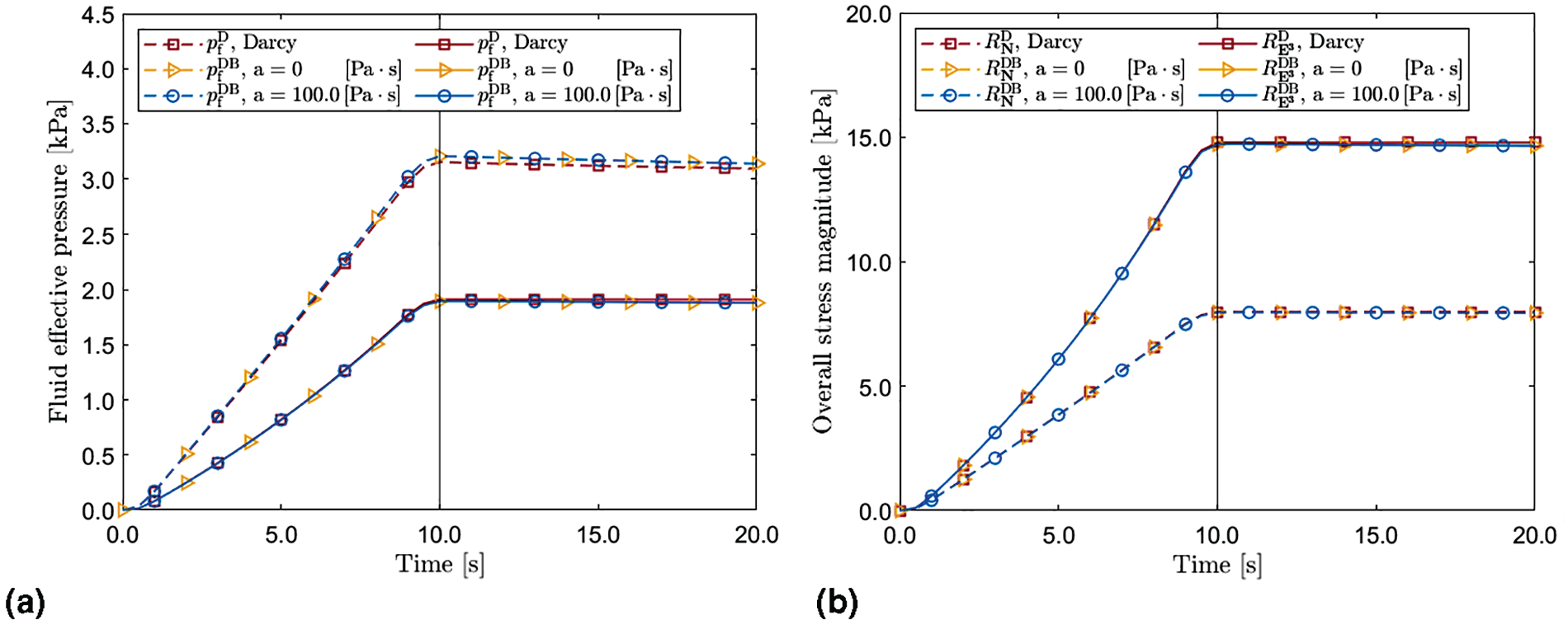
The purpose of this benchmark is to evaluate how switching from Darcy’s model to the Darcy–Brinkman model presented in our work influences the fluid pressure and the overall stress in the considered specimen. To this end, we select some representative points of the specimen. In particular, we discuss the role of the Brinkman second viscosity $\mathfrak{a}$ (referred to as the “volumetric fluid viscosity coefficient” in Table 1), since, in our model, the stress associated with it is nonzero in spite of the incompressibility of the fluid phase. This is a major difference with respect to the Darcy–Brinkman models of porous media that do not account for the deformation of the solid matrix and for the spatial variability of the porosity. Indeed, in these models, the fluid phase velocity field turns out to be divergence-free and the fluid Cauchy stress tensor becomes ${\mathit{\sigma }}_{\mathrm{f}}=2{\varphi }_{\mathrm{f}}\mathfrak{b}\mathrm{sym}(\mathit{g}\mathrm{grad}{\mathit{v}}_{\mathrm{f}}){\mathit{g}}^{-1}$ , where $\mathrm{grad}{\mathit{v}}_{\mathrm{f}}$ is deviatoric. In our framework, instead, ${\mathit{\sigma }}_{\mathrm{f}}$ is given by equation (63), since $\mathrm{div}{\mathit{v}}_{\mathrm{f}}$ is nonzero as a consequence of the deformation of the solid phase and variability of the medium’s porosity.

Figure 1. In Figure 1(a), we plot the fluid effective pressure field $p_{\mathrm{f}}$ (in Darcy’s case, $p_{\mathrm{f}}\equiv {\varphi }_{\mathrm{f}}p$ ) versus time, evaluated both at the middle point $X_{\mathrm{U}}$ of the upper interface ${\mathrm{\Gamma }}_{\mathrm{U}}$ between the specimen and the upper plate (dashed lines) and at the center of the specimen, $X_{\mathrm{C}}$ (solid lines).

Figure 1.

Left panel: fluid effective pressure $p_{\mathrm{f}}$ (see equation (66)) evaluated at the middle point $X_{\mathrm{U}}$ of the upper surface ${\mathrm{\Gamma }}_{\mathrm{U}}$ of the specimen (dashed lines), and at the center of the specimen $X_{\mathrm{C}}$ (solid lines). Right panel: overall stress magnitudes $R_{\mathit{N}}$ (see equation (75a)), evaluated at the middle point $X_{\mathrm{U}}$ of the upper surface ${\mathrm{\Gamma }}_{\mathrm{U}}$ of the specimen (dashed lines), and $R_{{\mathit{E}}^3}$ (see equation (75b)), evaluated at the center of the specimen $X_{\mathrm{C}}$ (solid lines). We consider three cases for the fluid flow: Darcian regime (“D”); Darcy–Brinkman model (“DB”) with $\mathfrak{a}=0\mathrm{Pa}\cdot \mathrm{s}$ ; and Darcy–Brinkman model (“DB”) with $\mathfrak{a}=100.0\mathrm{Pa}\cdot \mathrm{s}$ . (a) Fluid effective pressure $p_{\mathrm{f}}$ at $X_{\mathrm{U}}\in {\mathrm{\Gamma }}_{\mathrm{U}}$ and at $X_{\mathrm{C}}$ (no remodeling). (b) Overall stress magnitudes $R_{\mathit{N}}$ at $X_{\mathrm{U}}\in {\mathrm{\Gamma }}_{\mathrm{U}}$ and $R_{{\mathit{E}}^3}$ at $X_{\mathrm{C}}$ (no remodeling).

In Figure 1(b), we plot the time trend of the following overall stress magnitudes:

$$\begin{array}{ccccc}\hfill & R_{\mathit{N}}:=\parallel \{-\mathrm{Jp}{\mathit{F}}^{-\mathrm{T}}+{\hat{\mathit{P}}}_{\mathrm{s}}\circ (\mathit{F},{\mathit{F}}_{\gamma })+(J-{\mathrm{\Phi }}_{\mathrm{sR}})(\hat{\mathbb{V}}\circ \mathit{F}):\mathrm{Grad}{\mathit{V}}_{\mathrm{f}}\}\mathit{N}\parallel ,\hfill & \hfill & \mathrm{on}{\mathrm{\Gamma }}_{\mathrm{U}},\hfill & \hfill \end{array}$$

(75a)

$$\begin{array}{ccccc}\hfill & R_{{\mathit{E}}^3}:=\parallel \{-\mathrm{Jp}{\mathit{F}}^{-\mathrm{T}}+{\hat{\mathit{P}}}_{\mathrm{s}}\circ (\mathit{F},{\mathit{F}}_{\gamma })+(J-{\mathrm{\Phi }}_{\mathrm{sR}})(\hat{\mathbb{V}}\circ \mathit{F}):\mathrm{Grad}{\mathit{V}}_{\mathrm{f}}\}{\mathit{E}}^3\parallel ,\hfill & \hfill & \mathrm{on}{\mathrm{\Gamma }}_{\mathrm{C}},\hfill & \hfill \end{array}$$

(75b)

where N is the field of co-normals associated with ${\mathrm{\Gamma }}_{\mathrm{U}}$ and ${\mathit{E}}^3$ is the unit co-vector field of the basis ${\{{\mathit{E}}^A\}}_{A=1}^3$ , taken as the field of co-normals associated with the surface ${\mathrm{\Gamma }}_{\mathrm{C}}$ passing through $X_{\mathrm{C}}$ and orthogonal to the specimen’s symmetry axis. We evaluate $R_{\mathit{N}}$ at $X_{\mathrm{U}}$ and $R_{{\mathit{E}}^3}$ at $X_{\mathrm{C}}$ .

For the simulations that involve the Darcy–Brinkman model, we observe the response of the system for $\mathfrak{a}=0\mathrm{Pa}\cdot \mathrm{s}$ and for $\mathfrak{a}=100.0\mathrm{Pa}\cdot \mathrm{s}$ . The reason for choosing these values, which, to our knowledge, are not supported by experimental data, is to estimate the impact of the parameter $\mathfrak{a}$ on $p_{\mathrm{f}}$ , $R_{\mathit{N}}$ , and $R_{{\mathit{E}}^3}$ . For this purpose, we consider both $\mathfrak{a}=0\mathrm{Pa}\cdot \mathrm{s}$ and $\mathfrak{a}=100.0\mathrm{Pa}\cdot \mathrm{s}$ , which is five orders of magnitude greater than $\mathfrak{b}$ and much bigger than the volume viscosity coefficient of fluids that are often regarded as incompressible in biological media (about four orders of magnitude greater than water volume viscosity at $25^{\circ }\mathrm{C}$ ).

We denote by $p_{\mathrm{f}}^{\mathrm{D}}$ , $R_{\mathit{N}}^{\mathrm{D}}$ and $R_{{\mathit{E}}^3}^{\mathrm{D}}$ the curves obtained by using Darcy’s model, and by $p_{\mathrm{f}}^{\mathrm{DB}}$ , $R_{\mathit{N}}^{\mathrm{DB}}$ and $R_{{\mathit{E}}^3}^{\mathrm{DB}}$ those obtained by switching to the Darcy–Brinkman model.

Figure 1(a) and (b) compare the time trends of $p_{\mathrm{f}}^{\mathrm{D}}$ , $R_{\mathit{N}}^{\mathrm{D}}$ and $R_{{\mathit{E}}^3}^{\mathrm{D}}$ (squares) with those of $p_{\mathrm{f}}^{\mathrm{DB}}$ , $R_{\mathit{N}}^{\mathrm{DB}}$ and $R_{{\mathit{E}}^3}^{\mathrm{DB}}$ for $\mathfrak{a}=0\mathrm{Pa}\cdot s$ (triangles) and $\mathfrak{a}=100.0\mathrm{Pa}\cdot s$ (circles). In Figure 1(a), the transition from the Darcian model to the Darcy–Brinkman model produces, for both values of $\mathfrak{a}$ , appreciable changes in the values of $p_{\mathrm{f}}$ only at $X_{\mathrm{U}}$ (dashed lines) and for $t\in ]t_{\mathrm{r}},t_{\mathrm{e}}[$ , while it yields very modest differences at $X_{\mathrm{C}}$ and over the same time window (solid lines). In Figure 1(b), instead, no remarkably appreciable differences are observed in the time trends of $R_{\mathit{N}}$ and $R_{{\mathit{E}}^3}$ , regardless of the values attributed to $\mathfrak{a}$ . These results could be related to the simple geometry of the contact zones between the specimen and the plates, which do not give rise to particularly noticeable boundary effects (at least, as long as remodeling is deactivated). Hence, for the next simulations we take $\mathfrak{a}=0\mathrm{Pa}\cdot \mathrm{s}$ .

5.3.2. Second benchmark: Darcy–Brinkman model with strain-gradient remodeling

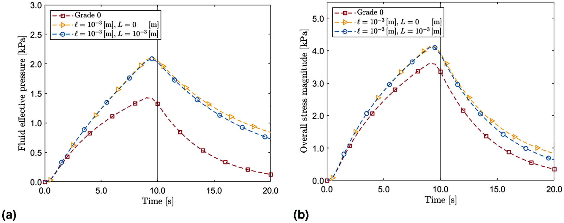
We discuss the evolution of the system with remodeling. We compare three cases: (i) the flow is in Darcian regime and the remodeling distortions evolve according to a grade-0 theory in ${\mathit{F}}_{\gamma }$ , i.e., with $\mathrm{Grad}{\tilde{\mathit{D}}}_{\gamma }$ and $\mathfrak{B}$ absent from equation (69c), which thus reduces to ${\overline{S}}_{\mathrm{y}}{\tilde{\mathit{D}}}_{\gamma }^{\ast }={\tilde{\mathit{A}}}^{♯}$ , with $\mathit{A}={\mathit{F}}_{\gamma }^{-\mathrm{T}}[{\mathit{F}}^{\mathrm{T}}{\mathit{P}}_{\mathrm{s}}]{\mathit{F}}_{\gamma }^{\mathrm{T}}$ ; (ii) the fluid obeys the Darcy–Brinkman model, but the non-dissipative effects of remodeling associated with $W_{\mathrm{sD}}$ are neglected, which amounts to prescribe $L=0\mathrm{m}$ ; (iii) the full IBVP of Section 5 is solved.

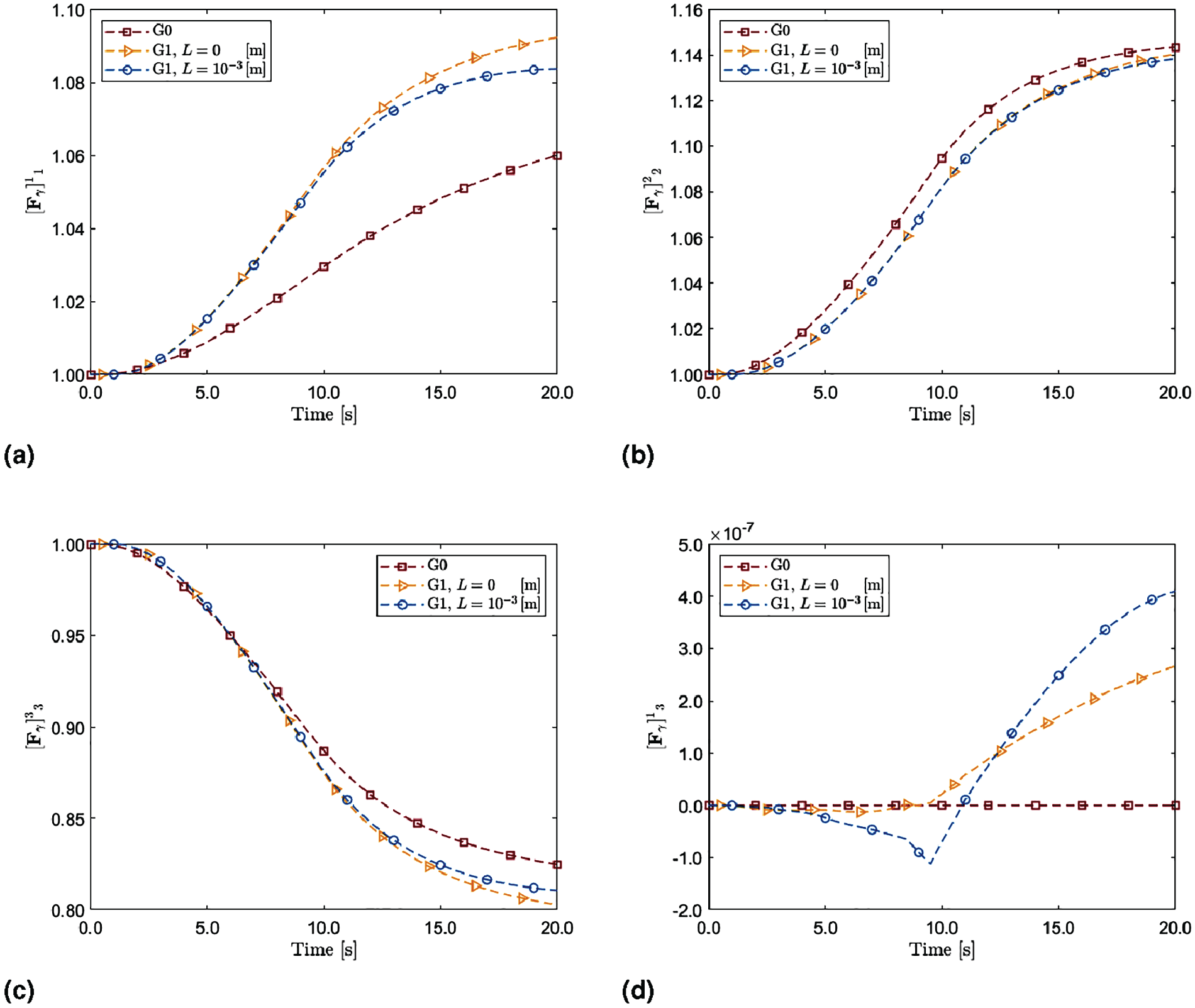
Figure 2. In Figure 2(a) we report the evaluation of the fluid effective pressure $p_{\mathrm{f}}$ in the middle point $X_{\mathrm{U}}$ of the specimen’s upper surface ${\mathrm{\Gamma }}_{\mathrm{U}}$ , and over the time interval $[0\mathrm{s},t_{\mathrm{e}}=20\mathrm{s}]$ . In Figure 2(b) we show the evaluation of $R_{\mathit{N}}$ at the same point and over the same time interval. In both figures, we observe changes in the time trend when we pass from Darcy’s model and grade-0 remodeling, i.e., the “Grade-0” case, to the Darcy–Brinkman model and grade-1 remodeling, i.e., the “Grade-1” case (identified by the values given to the length scales ℓ and L). For conciseness, we denote by $p_{\mathrm{f}}^{\mathrm{G}0}$ and $R_{\mathit{N}}^{\mathrm{G}0}$ the curves referring to the Grade-0 case (squares) and by $p_{\mathrm{f}}^{\mathrm{G}1}$ and $R_{\mathit{N}}^{\mathrm{G}1}$ those referring to the Grade-1 case (triangles and circles). Note that, for all these simulations, the Brinkman viscosity $\mathfrak{a}$ is set equal to zero, while $\mathfrak{b}$ is given the value reported in Table 1.

Figure 2.

Left panel: fluid effective pressure $p_{\mathrm{f}}$ (see equation (66)) evaluated at the middle point $X_{\mathrm{U}}$ of the upper surface ${\mathrm{\Gamma }}_{\mathrm{U}}$ of the specimen. Right panel: overall stress magnitude $R_{\mathit{N}}$ (see equation (75a)) evaluated at the middle point $X_{\mathrm{U}}$ of the upper surface ${\mathrm{\Gamma }}_{\mathrm{U}}$ of the specimen. The solid vertical line at $t=t_{\mathrm{r}}=10\mathrm{s}$ indicates the instant of time in which the compressive ramp exerts the maximum displacement. Because of the regularization of the compressive ramp, the maxima of all the plotted curves are attained at time $t_{\max }=t_{\mathrm{r}}-1=9\mathrm{s}$ . (a) Fluid effective pressure $p_{\mathrm{f}}$ at $X_{\mathrm{U}}\in {\mathrm{\Gamma }}_{\mathrm{U}}$ (case with remodeling). (b) Overall stress magnitudes $R_{\mathit{N}}$ at $X_{\mathrm{U}}\in {\mathrm{\Gamma }}_{\mathrm{U}}$ (case with remodeling).

A noticeable result is that, when remodeling is activated, the values of both $p_{\mathrm{f}}$ and $R_{\mathit{N}}$ are appreciably smaller than those appearing in the case in which remodeling is switched off. This behavior is expected as a consequence of the mitigating effect that remodeling has on the distribution of the stresses in a medium. Moreover, the presence of remodeling accelerates the relaxation of all the curves plotted in Figure 2(a) and (b) towards a state of lower pressure and stress.

Aside from the considerations made above, to us one result is noteworthy: the curves of $p_{\mathrm{f}}^{\mathrm{G}1}$ and $R_{\mathit{N}}^{\mathrm{G}1}$ , obtained for $L=0\mathrm{m}$ and $L=10^{-3}\mathrm{m}$ , share a time trend qualitatively similar to those of $p_{\mathrm{f}}^{\mathrm{G}0}$ and $R_{\mathit{N}}^{\mathrm{G}0}$ , although there is an appreciable difference after a certain instant of time greater than the instant $t_{\max }$ at which all the curves attain their maxima. In fact, for $L=0\mathrm{m}$ , the values of $p_{\mathrm{f}}^{\mathrm{G}1}$ and of $R_{\mathit{N}}^{\mathrm{G}1}$ (triangles) are higher than the corresponding ones obtained for $L=10^{-3}\mathrm{m}$ (circles). This means that, although the Grade-1 curves are all above the Grade-0 ones, the activation of the length scale L, related to the non-dissipative parts of ${\mathit{Y}}_{\mathrm{u}}$ and ${\mathbb{Y}}_{\mathrm{u}}$ , plays a mitigating role both on the pressure and on the overall stress, thereby accelerating their relaxation.

Figure 3. In Figure 3(a)–(d) we plot the time trends of the radial, circumferential, and axial components of ${\mathit{F}}_{\gamma }$ as well as of the radial-axial (13-)component of ${\mathit{F}}_{\gamma }$ . All these evaluations are taken at the point $X_{\mathrm{L}}\in {\mathrm{\Gamma }}_{\mathrm{L}}$ of coordinates $(5.0,0.0,5.0)\mathrm{mm}$ , lying at half of the height of the specimen’s lateral boundary, ${\mathrm{\Gamma }}_{\mathrm{L}}$ . We indicate with ${\mathit{F}}_{\gamma }^{\mathrm{G}0}$ the remodeling tensor related to the Grade-0 case (squares), and with ${\mathit{F}}_{\gamma }^{\mathrm{G}1}$ the same quantity obtained within the Grade-1 case (circles for non-vanishing “defect” free energy density $W_{\mathrm{sD}}$ , i.e., $L=10^{-3}\mathrm{m}$ , and triangles for vanishing $W_{\mathrm{sD}}$ , i.e., $L=0\mathrm{m}$ ).

Figure 3.

Evolution of the radial (a), circumferential (b), axial (c), and radial-axial shear component of ${\mathit{F}}_{\gamma }$ (d) at the point $X_{\mathrm{L}}$ of coordinates $(5.0,0.0,5.0)\mathrm{mm}$ of the specimen’s lateral surface ${\mathrm{\Gamma }}_{\mathrm{L}}$ . (a) 11-component of ${\mathit{F}}_{\gamma }$ at $X_{\mathrm{L}}\in {\mathrm{\Gamma }}_{\mathrm{L}}$ , (b) 22-component of ${\mathit{F}}_{\gamma }$ at $X_{\mathrm{L}}\in {\mathrm{\Gamma }}_{\mathrm{L}}$ , (c) 33-component of ${\mathit{F}}_{\gamma }$ at $X_{\mathrm{L}}\in {\mathrm{\Gamma }}_{\mathrm{L}}$ and (d) 13-component of ${\mathit{F}}_{\gamma }$ at $X_{\mathrm{L}}\in {\mathrm{\Gamma }}_{\mathrm{L}}$ .

A relevant feature of Figure 3 is that, after a certain instant of time in the interval $[0\mathrm{s},5\mathrm{s}]$ , ${[{\mathit{F}}_{\gamma }^{\mathrm{G}1}{]}^1}_1$ becomes larger than ${[{\mathit{F}}_{\gamma }^{\mathrm{G}0}{]}^1}_1$ both for $L=0\mathrm{m}$ and for $L=10^{-3}\mathrm{m}$ (see Figure 3(a)), while ${[{\mathit{F}}_{\gamma }^{\mathrm{G}1}{]}^2}_2$ remains smaller than ${[{\mathit{F}}_{\gamma }^{\mathrm{G}0}{]}^2}_2$ for almost the entire duration of the simulation (see Figure 3(b)), although, at $t=t_{\mathrm{e}}$ , ${[{\mathit{F}}_{\gamma }^{\mathrm{G}1}{]}^2}_2$ for $L=0\mathrm{m}$ (triangles) comes closer to the value attained by ${[{\mathit{F}}_{\gamma }^{\mathrm{G}0}{]}^2}_2$ at $t_{\mathrm{e}}$ (squares). Moreover, both for $L=0\mathrm{m}$ and for $L=10^{-3}\mathrm{m}$ (triangles and circles), the curves of ${[{\mathit{F}}_{\gamma }^{\mathrm{G}1}{]}^3}_3$ intersect the curve of ${[{\mathit{F}}_{\gamma }^{\mathrm{G}0}{]}^3}_3$ (squares) at an instant of time $t_{\ast }$ in the interval $]5\mathrm{s},t_{\mathrm{r}}-1[$ , and, in particular, they attain smaller values after $t_{\ast }$ (see Figure 3(c)). Finally, both for the Grade-0 case and for the Grade-1 case, the values of ${[{\mathit{F}}_{\gamma }{]}^1}_3$ are negligibly small with respect to the diagonal components of the remodeling tensor (see Figure 3(d)). Although we expect this result, due to the symmetries of the problem under investigation, we notice that, while ${[{\mathit{F}}_{\gamma }^{\mathrm{G}0}{]}^1}_3$ is zero (in fact, its simulated values are of the order of $10^{-16}$ ), ${[{\mathit{F}}_{\gamma }^{\mathrm{G}1}{]}^1}_3$ is of the order of $10^{-7}$ .

We remark that, in Figure 3(a), (c) and (d), switching from $L=0\mathrm{m}$ to $L=10^{-3}\mathrm{m}$ yields appreciable differences in the examined components of the remodeling tensor, while these differences are less marked in Figure 3(b). In particular, in the Grade-1 model, and during the relaxation phase, the presence of the energetic contributions to ${\mathit{Y}}_{\mathrm{u}}$ and ${\mathbb{Y}}_{\mathrm{u}}$ due to $L=10^{-3}\mathrm{m}$ (circles) tend to decrease ${[{\mathit{F}}_{\gamma }^{\mathrm{G}1}{]}^1}_1$ and ${[{\mathit{F}}_{\gamma }^{\mathrm{G}1}{]}^2}_2$ and to increase ${[{\mathit{F}}_{\gamma }^{\mathrm{G}1}{]}^3}_3$ with respect to the case $L=0\mathrm{m}$ . Hence, we conclude that these energetic contributions tend to hinder these components of the remodeling tensor near the lateral boundary.

Figure 4. In Figure 4(a), we report the 33-component of ${\mathit{F}}_{\gamma }^{\mathrm{G}1}$ and ${\mathit{F}}_{\gamma }^{\mathrm{G}0}$ at $t=t_{\mathrm{r}}=10\mathrm{s}$ and at $t=t_{\mathrm{e}}=20\mathrm{s}$ (final time of observation). The curves of ${[{\mathit{F}}_{\gamma }^{\mathrm{G}0}{]}^3}_3$ (squares) take on unitary values at the extrema of the spatial interval $[0\mathrm{mm},10\mathrm{mm}]$ , corresponding to the middle points of the bottom and upper surfaces, denoted by $X_{\mathrm{B}}=(0,0,0)\mathrm{mm}$ and $X_{\mathrm{U}}=(0,0,10)\mathrm{mm}$ , respectively. The evolution of the remodeling is testified by the fact that, at the end of the simulation, i.e., for $t=t_{\mathrm{e}}$ , the curve of ${[{\mathit{F}}_{\gamma }^{\mathrm{G}0}{]}^3}_3$ (solid line marked by squares) is below the one obtained for $t=t_{\mathrm{r}}$ (dashed line marked by squares). We notice that the derivative of ${[{\mathit{F}}_{\gamma }^{\mathrm{G}0}{]}^3}_3$ along the axial direction, and evaluated at the points $X_{\mathrm{B}}$ and $X_{\mathrm{U}}$ , is nonzero.

Figure 4.

Left panel: comparison of the components ${[{\mathit{F}}_{\gamma }{]}^3}_3$ computed within the Grade-0 model, i.e., ${[{\mathit{F}}_{\gamma }^{\mathrm{G}0}{]}^3}_3$ , with the same quantities computed within the Grade-1 model, i.e., ${[{\mathit{F}}_{\gamma }^{\mathrm{G}1}{]}^3}_3$ ; the evaluation is done along the symmetry axis of the specimen. Right panel: comparison of the components ${[{\mathit{F}}_{\gamma }{]}^1}_1$ computed within the Grade-0 model, i.e., ${[{\mathit{F}}_{\gamma }^{\mathrm{G}0}{]}^1}_1$ , with the same quantities computed within the Grade-1 model, i.e., ${[{\mathit{F}}_{\gamma }^{\mathrm{G}1}{]}^1}_1$ ; the evaluation is done along the radial segment comprised between the points $(0.0,0.0,5.0)\mathrm{mm}$ and $(5.0,0.0,5.0)\mathrm{mm}$ . In both panels, the cases $L=0\mathrm{m}$ and $L=10^{-3}\mathrm{m}$ characterize the Grade-1 model. (a) Symmetry axis, 33-component of ${\mathit{F}}_{\gamma }$ . (b) Radial segment, 11-component of ${\mathit{F}}_{\gamma }$ .

A quite different behavior can be observed for ${[{\mathit{F}}_{\gamma }^{\mathrm{G}1}{]}^3}_3$ . In this case, indeed, although the curves plotted for $t=t_{\mathrm{r}}=10\mathrm{s}$ (dashed lines marked with triangles and circles) and for $t=t_{\mathrm{e}}=20\mathrm{s}$ (solid lines marked with triangles and circles) are symmetric with respect to the straight line of equation $X^3=5\mathrm{mm}$ (corresponding to transverse plane passing through $X_{\mathrm{C}}$ ), the derivatives of ${[{\mathit{F}}_{\gamma }^{\mathrm{G}1}{]}^3}_3$ along the axial direction, and evaluated at the points $X_{\mathrm{B}}$ and $X_{\mathrm{U}}$ , are (almost) zero, in accordance with the boundary conditions ${\mathbb{Y}}_{\mathrm{u}}\mathit{N}=\mathit{O}$ (see equation (68)). This is, in fact, an effect of the boundary that is not visible for the Grade-0 model.

In Figure 4(b) we show the radial component ${[{\mathit{F}}_{\gamma }^{\mathrm{G}1}{]}^1}_1$ and ${[{\mathit{F}}_{\gamma }^{\mathrm{G}0}{]}^1}_1$ . As one expects, for each curve, the maximum is attained at the symmetry axis.

It is worth mentioning that, as shown in Figure 4(a) and (b), in the inner region of the specimen the components ${[{\mathit{F}}_{\gamma }^{\mathrm{G}1}{]}^3}_3$ and ${[{\mathit{F}}_{\gamma }^{\mathrm{G}1}{]}^1}_1$ for $t=t_{\mathrm{r}}=10\mathrm{s}$ (dashed lines marked with triangles and circles) assume values closer to unity than their Grade-0 counterparts do. However, for $t=t_{\mathrm{e}}=20\mathrm{s}$ , the values of ${[{\mathit{F}}_{\gamma }^{\mathrm{G}1}{]}^3}_3$ and ${[{\mathit{F}}_{\gamma }^{\mathrm{G}1}{]}^1}_1$ (solid lines marked with triangles and circles) become very similar to the ones predicted by the Grade-0 theory. This suggests that ${[{\mathit{F}}_{\gamma }^{\mathrm{G}1}{]}^3}_3$ and ${[{\mathit{F}}_{\gamma }^{\mathrm{G}1}{]}^1}_1$ distance themselves from unity on the interval $[t_{\mathrm{r}},t_{\mathrm{e}}]$ a little bit more than their Grade-0 counterparts.

6. Concluding remarks

We have studied the mechanics of a multicellular aggregate within a strain-gradient theory of remodeling (re-proposed from the work by Gurtin and Anand [38]) and a Darcy–Brinkman model for the interstitial fluid. This framework has been obtained by selecting the motion of the solid phase, the velocity field of the fluid phase and the remodeling tensor as basic kinematic fields for the system under consideration.

Our results show that, in the absence of remodeling, the Darcy–Brinkman model for simulating the compression test of a homogeneous and isotropic cylindrical specimen leads to rather modest variations of the fluid effective pressure and to almost no appreciable changes in the stress distribution as compared with the same quantities predicted by standard Darcy’s law. As discussed in the presentation of the figures, this could be partially imputable to the simple geometry of the specimen’s boundary and to the loading conditions, which do not alter such geometry, thereby not giving room to strong boundary effects. In this respect, the benchmark test that we have simulated may seem to be inappropriate for justifying the Brinkman correction. However, the fact that there appear differences in the fluid effective pressure already in the simple situation analyzed in our work suggests that the Darcy–Brinkman model could become important in situations generating strong gradients of the fluid velocity field. These could involve, for instance, twist tests or indentation tests, in which the original geometry of the specimen is remarkably modified, or transport problems in which the fluid is injected into the tested medium.

A different consideration concerns the role of the bulk viscosity parameter $\mathfrak{a}$ . For the values considered in our work, $\mathfrak{a}$ does not alter significantly the evolution of the system, but we have not assessed yet whether, from the point of view of computing, $\mathfrak{a}$ could stabilize the numerical solution.

These considerations notwithstanding, appreciable differences in the fluid effective pressure, stress distribution within the specimen, and in the components of the remodeling tensor emerge when the Grade-0 model is compared with the Grade-1 model. In this respect, we remark that, while strain-gradient theories in the anelastic descriptor have been historically introduced to account for size effects in crystalline solids, and their importance cannot be understated (see e.g. the review by Voyiadjis and Song [37]), the determination of the phenomenological length scales ℓ and L in biological media is still an open problem. To the authors’ knowledge, there is a lack of experimental protocols for the identification of size effects in biological tissues, with a notable exception being the study of the mechanics of trabecular bone [97,98]. In fact, following the opening of a crack, the neighboring region of the bone undergoes a remodeling process by developing plastic-like distortions and forming the so called “plastic zone” [97], which can be regarded as a size effect encompassing various elementary cells of a bone [97,98] and determines a dissipative phenomenological length scale that can be estimated [97].

We conclude this discussion on the Darcy–Brinkman model with a remark. Auriault [99] obtains the Darcy–Brinkman model starting from Stokes’ equation as a result of an up-scaling procedure that involves the asymptotic expansion of the fields of fluid pressure and velocity in a non-deforming porous medium made of “swarms of fixed particles or fixed beds of fibers at very low concentration, only, and under precise conditions” [99]. In this case, Auriault [99] finds that the so-called Brinkman viscosity equals the true viscosity of the fluid. However, he also warns that “for isotropic and macroscopically homogeneous porous media […] Brinkman’s equation has no physical background” [99]. While bearing this criticism in mind, we are aware of studies suggesting the usefulness of the Darcy–Brinkman model in addressing biomechanical problems [40]. Since biological porous media, especially when subjected to remodeling, have an internal structure that evolves and may deviate somewhat from the one of “macroscopically homogeneous porous media” [99], examining the influence of Brinkman’s correction on the flow and its interaction with remodeling could deserve investigations. This has indeed motivated the present work and some results have been discussed in the previous section. Another case worthy of attention is provided by fiber-reinforced composites, which, besides the remodeling of the matrix, undergo also the reorientation of the fibers. Although the Darcy–Brinkman model in fiber-reinforced media is present in the literature (see, e.g., Hwang and Advani [100]), it could be useful to investigate how the non-spherical and dissipative stress tensor predicted by the Brinkman model couples with the fibers’ distribution in the medium and whether it plays a role in the reorientation of the fibers themselves [46]. Clearly, all these considerations are at the moment conjectures and await experimental verification.