Major symmetry of the induced tangent stiffness tensor for the Zaremba–Jaumann rate and Kirchhoff stress in hyperelasticity: Two different approaches

Abstract

We recall in this note that the induced tangent stiffness tensor ${\mathbb{H}}_{\mathrm{\tau }}^{\mathrm{ZJ}}\left(\tau \right)$ appearing in a hypoelastic formulation based on the Zaremba–Jaumann corotational derivative and the rate constitutive equation for the Kirchhoff stress tensor τ is minor and major symmetric if the Kirchhoff stress τ is derived from an elastic potential $W\left(F\right)$ . This result is vaguely known in the literature. Here, we expose two different notational approaches which highlight the full symmetry of the tangent stiffness tensor ${\mathbb{H}}_{\mathrm{\tau }}^{\mathrm{ZJ}}\left(\tau \right)$ . The first approach is based on the direct use of the definition of each symmetry (minor and major), i.e., via contractions of the tensor with the deformation rate tensor D. The second approach aims at finding an absolute expression of the tensor ${\mathbb{H}}_{\mathrm{\tau }}^{\mathrm{ZJ}}\left(\tau \right)$ , by means of special tensor products and their symmetrisations. In some past works, the major symmetry of ${\mathbb{H}}_{\mathrm{\tau }}^{\mathrm{ZJ}}\left(\tau \right)$ has been missed because not all necessary symmetrisations were applied. The analogous tangent stiffness tensor ${\mathbb{H}}^{\mathrm{ZJ}}\left(\sigma \right)$ , relating the Cauchy stress tensor σ to the Zaremba–Jaumann corotational derivative is also obtained, with both methods used for ${\mathbb{H}}_{\mathrm{\tau }}^{\mathrm{ZJ}}\left(\tau \right)$ . The approach is exemplified for the isotropic Hencky energy. Corresponding stability checks of software packages are shortly discussed.

1. Introduction

1.1. Recap on rate-formulations for nonlinear elasticity

Nonlinear elasticity is today an integral part of continuum mechanical modelling. The basic framework is definitely established [1–9]. Here, we are interested in a question occurring when implementing a finite element model (FEM)-code for nonlinear elasticity.

While the overwhelming current trend is to use a totally Lagrangean approach, providing the direct discretization of the equilibrium equation

$$\mathrm{Div}{S}_1\left(F\right)=f$$

(1)

on the reference configuration $\mathrm{\Omega }\subset {\mathbb{R}}^3$ where $\phi :\mathrm{\Omega }\subset {\mathbb{R}}^3\to {\mathbb{R}}^3$ is the deformation, $F=\mathrm{D}\phi \in \mathrm{G}{\mathrm{L}}^{+}\left(3\right)$ is the deformation gradient (the Fréchet-derivative of φ) and $S_1\left(F\right)$ is the (non-symmetric) first Piola–Kirchhoff stress, many established software packages like Abaqus™, Ansys™ ¹ , LS-DYNA, and so on discretise a rate-type formulation on the current configuration $\phi \left(\mathrm{\Omega }\right)$ , and the constitutive law is accordingly an expression relating increments of spatial stress to increments of spatial strain. For example, Abaqus™ in its UMAT subroutine requires the rate-formulation for the Kirchhoff stress τ expressed with the Zaremba–Jaumann rate.

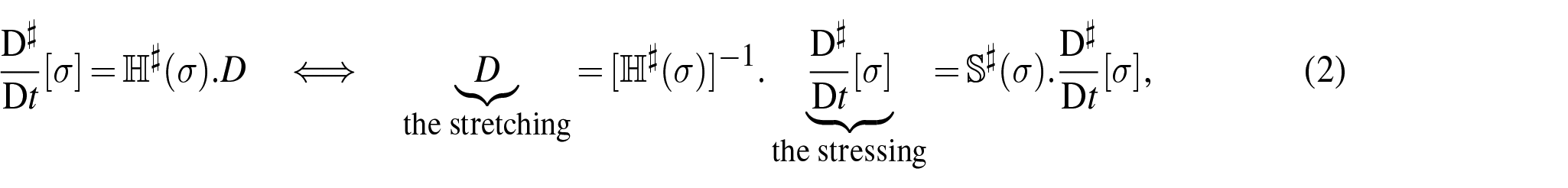
Here, it has to be remarked that any hyper- or Cauchy-elastic law on the reference configuration can be equivalently expressed in a rate-type or hypoelastic format. More precisely, a hypo-elastic material, in the sense of Truesdell [10] and Noll [11], obeys a constitutive law of the form

$$\frac{{\mathrm{D}}^{♯}}{\mathrm{D}t}[\sigma ]={\mathbb{H}}^{♯}\left(\sigma \right).D\iff \underset{\mathrm{the}\mathrm{stretching}}{\underbrace{D}}=[{\mathbb{H}}^{♯}\left(\sigma \right){]}^{-1}.\underset{\mathrm{the}\mathrm{stressing}}{\underbrace{\frac{{\mathrm{D}}^{♯}}{\mathrm{D}t}[\sigma ]}}={\mathbb{S}}^{♯}\left(\sigma \right).\frac{{\mathrm{D}}^{♯}}{\mathrm{D}t}[\sigma ],$$

(2)

where

• $\frac{{\mathrm{D}}^{♯}}{\mathrm{D}t}[\sigma ]$ is an appropriate objective rate of the Cauchy stress tensor σ,

• ${\mathbb{H}}^{♯}\left(\sigma \right)$ is a constitutive fourth-order tangent stiffness tensor,

• ${\mathbb{S}}^{♯}\left(\sigma \right)$ = $[{\mathbb{H}}^{♯}\left(\sigma \right){]}^{-1}$ is a constitutive fourth-order tangent compliance tensor and

• D = sym D_ξv = sym L is the Eulerian strain rate tensor, measuring the spatial rate of deformation or “stretching”, where v describes the spatial velocity at a point ξ in the current configuration, and $L={\mathrm{D}}_{\xi }v=\stackrel{·}{F}{F}^{-1}$ is the velocity gradient.

Hence, the elastic stretching D depends only on the current stress level σ and the rate of stress $\frac{{\mathrm{D}}^{♯}}{\mathrm{D}t}[\sigma ]$ as seen by the objective derivative.

As for time derivatives $\frac{{\mathrm{D}}^{♯}}{\mathrm{D}t}[\sigma ]$ of the Cauchy stress tensor σ, there are many different possible choices (see, e.g., also the related works by Xiao et al. [12, 13], Bonet and Wood [14], Aubram [15], Bellini and Federico [16], Palizi et al. [17], Fiala [18, 19]), Govindjee [20], Korobeynikov [21, 22], Pinsky et al. [23], and the book by Ogden [6]).

This framework admits usually two basic choices. We can express the rate-form constitutive law in terms of the Cauchy stress σ, or alternatively in terms of the Kirchhoff stress (the weighted Cauchy stress)

$$\tau =\det F·\sigma =J·\sigma .$$

(3)

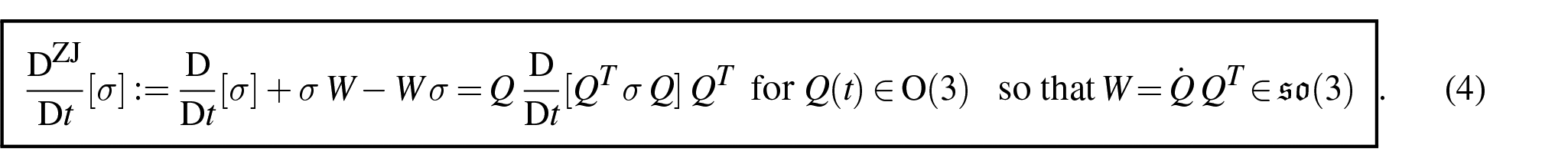
On the contrary, we are free to choose the objective derivatives [24–26]. Provided the induced tangent stiffness tensor ${\mathbb{H}}^{♯}$ in equation (2) is adjusted properly, all formulations are fully equivalent. Here, we consider primarily the combination of the Kirchhoff-stress τ with the corotational Zaremba–Jaumann rate [24, 27, 28], using the vorticity tensor (or spin tensor) $W=\mathrm{skew}L,L=\stackrel{·}{F}{F}^{-1}$ ,

$$\frac{{\mathrm{D}}^{\mathrm{Z}\mathrm{J}}}{\mathrm{D}t}[\sigma ]:=\frac{\mathrm{D}}{\mathrm{D}t}[\sigma ]+\sigma W-W\sigma =Q\frac{\mathrm{D}}{\mathrm{D}t}[Q^T\sigma Q]Q^T\mathrm{for}Q\left(t\right)\in O\left(3\right)\mathrm{so}\mathrm{that}W=\stackrel{.}{Q}{Q}^T\in \mathfrak{s}\mathfrak{o}\left(3\right).$$

(4)

Neff et al. [26] have shown how to obtain the corresponding induced stiffness tensor ${\mathbb{H}}^{\mathrm{ZJ}}\left(\sigma \right)$ if $\sigma =\sigma \left(B\right)$ is given as an isotropic Cauchy elastic law. Indeed, for $\sigma \left(B\right)=\hat{\sigma }\left(\log B\right)$ , it holds

$${\mathbb{H}}^{\mathrm{ZJ}}\left(\sigma \right).D:={\mathrm{D}}_B\sigma \left(B\right).[\mathrm{BD}+\mathrm{DB}]={\mathrm{D}}_{\log B}\hat{\sigma }\left(\log B\right).{\mathrm{D}}_B\log B.\frac{{\mathrm{D}}^{\mathrm{ZJ}}}{\mathrm{D}t}[B]$$

(5)

together with

$$\frac{{\mathrm{D}}^{\mathrm{ZJ}}}{\mathrm{D}t}[\sigma ]={\mathbb{H}}^{\mathrm{ZJ}}\left(\sigma \right).D.$$

(6)

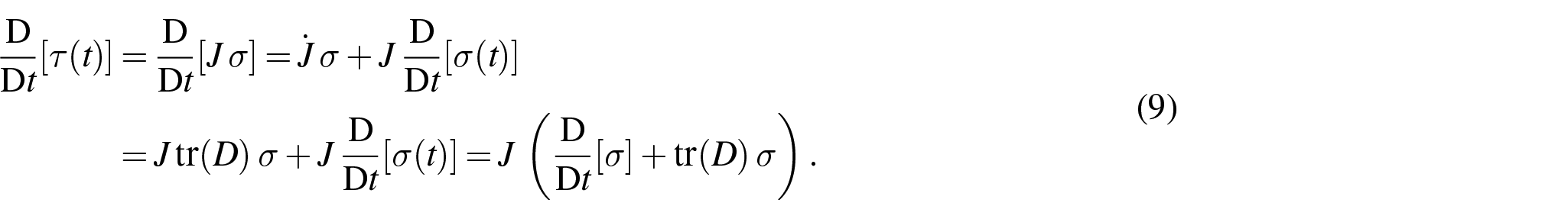
The constitutive law (6) can be converted into a rate-formulation for the Kirchhoff stress τ:

$$\frac{{\mathrm{D}}^{\mathrm{ZJ}}}{\mathrm{D}t}[\tau ]={\mathbb{H}}_{\tau }^{\mathrm{ZJ}}\left(\tau \right).D.$$

(7)

This will be recalled in the next section 1.2. It is then an observation, which while the fourth-order tensor ${\mathbb{H}}^{\mathrm{ZJ}}\left(\sigma \right)$ is in general not major-symmetric (but always minor symmetric), the corresponding induced stiffness tensor ${\mathbb{H}}_{\tau }^{\mathrm{ZJ}}\left(\tau \right)$ for the Kirchhoff stress will be major-symmetric provided $\tau =\tau \left(B\right)$ derives from hyperelasticity.

This will be shown by two different and complementing approaches, and this constitutes the major result of this contribution. Demonstrating all symmetries of the stiffness tensor ${\mathbb{H}}^{\mathrm{ZJ}}\left(\sigma \right)$ is important for two reasons. First, from the epistemological point of view, if a symmetry exists, it must be studied and accounted for. Second, from the computational point of view, a fourth-order tensor with major and both minor symmetries has 21 independent components, as opposed to the 36 of a fourth-order tensor with only the minor symmetries, and this reduces the memory allocation, which can be advantageous in large FEMs.

In addition, we will give an explicit example for the calculation of ${\mathbb{H}}^{\mathrm{ZJ}}\left(\sigma \right)$ and ${\mathbb{H}}_{\tau }^{\mathrm{ZJ}}\left(\tau \right)$ for the Hencky energy in section 2. Finally, we shortly discuss a customary stability check of Abaqus™ and Ansys™ in relation to the Hencky model.

1.2. Converting the hypoelastic formulation with Zaremba–Jaumann rate and Cauchy stress σ into an equivalent hypoelastic formulation for the Kirchhoff stress τ

Assume we know how to express the rate-formulation for the Cauchy stress σ and the Zaremba–Jaumann rate, i.e., we have

$$\frac{{\mathrm{D}}^{\mathrm{ZJ}}}{\mathrm{D}t}[\sigma ]={\mathbb{H}}^{\mathrm{ZJ}}\left(\sigma \right).D$$

(8)

and we know the fourth-order tensor ${\mathbb{H}}^{\mathrm{ZJ}}\left(\sigma \right)$ . Then it is easy to obtain the rate-formulation for the Kirchhoff stress τ, as is shown next.

We recall that $\tau =detF·\sigma =J·\sigma =F{S}_2{F}^T$ . Then

$$\begin{array}{c}\multicolumn{1}{c}{\frac{\mathrm{D}}{\mathrm{D}t}[\tau \left(t\right)]=\frac{\mathrm{D}}{\mathrm{D}t}[J\sigma ]=\stackrel{·}{J}\sigma +J\frac{\mathrm{D}}{\mathrm{D}t}[\sigma \left(t\right)]}\\ \multicolumn{1}{c}{=J\mathrm{tr}\left(D\right)\sigma +J\frac{\mathrm{D}}{\mathrm{D}t}[\sigma \left(t\right)]=J(\frac{\mathrm{D}}{\mathrm{D}t}[\sigma ]+\mathrm{tr}\left(\mathrm{D}\right)\sigma ).}\end{array}$$

(9)

Moreover

$$\frac{{\mathrm{D}}^{\mathrm{ZJ}}}{\mathrm{D}t}[\sigma ]=\frac{\mathrm{D}}{\mathrm{D}t}[\sigma ]+\sigma W-W\sigma \mathrm{and}\frac{{\mathrm{D}}^{\mathrm{ZJ}}}{\mathrm{D}t}[\sigma ]={\mathbb{H}}^{\mathrm{ZJ}}\left(\sigma \right).D$$

(10)

and ²

$$\begin{array}{c}\multicolumn{1}{c}{\frac{{\mathrm{D}}^{\mathrm{ZJ}}}{\mathrm{D}t}[\tau ]=\frac{{\mathrm{D}}^{\mathrm{ZJ}}}{\mathrm{D}t}[J\sigma ]=\frac{\mathrm{D}}{\mathrm{D}t}[J\sigma ]+\left(J\sigma \right)W-W\left(J\sigma \right)=J\frac{\mathrm{D}}{\mathrm{D}t}[\sigma ]+\stackrel{·}{J}\sigma +J\sigma W-JW\sigma }\\ \multicolumn{1}{c}{=J[\frac{\mathrm{D}}{\mathrm{D}t}[\sigma ]+\mathrm{tr}\left(\mathrm{D}\right)\sigma ]+J\sigma W-WJ\sigma =J[\frac{\mathrm{D}}{\mathrm{D}t}[\sigma ]+\sigma W-W\sigma ]+\mathrm{tr}\left(D\right)\tau }\\ \multicolumn{1}{c}{=J{\mathbb{H}}^{\mathrm{ZJ}}\left(\sigma \right).D+\mathrm{tr}\left(D\right)\tau =J\underset{=:\mathbb{D}.D}{\underbrace{[{\mathbb{H}}^{\mathrm{ZJ}}\left(\frac{1}{J}\tau \right).D+\frac{1}{J}\mathrm{tr}\left(D\right)\tau ]}}=:{\mathbb{H}}_{\tau }^{\mathrm{ZJ}}(\tau ;J).D}\\ \multicolumn{1}{c}{=J(\frac{\mathrm{D}}{\mathrm{D}t}[\sigma ]+\sigma W-W\sigma +\mathrm{tr}\left(\mathrm{D}\right)\sigma )=J\frac{{\mathrm{D}}^{\mathrm{Hencky}}}{\mathrm{D}t}[\sigma ]}\\ \multicolumn{1}{c}{=J\frac{{\mathrm{D}}^{\mathrm{Hencky}}}{\mathrm{D}t}\left[\frac{1}{J}\tau \right],(\mathrm{cf}.\mathrm{Korobeynikov}[22,\mathrm{p}.3879]).}\end{array}$$

(11)

It is engineering folklore that ${\mathbb{H}}_{\tau }^{\mathrm{ZJ}}\left(\tau \right)$ is a symmetric matrix viewed as a (self-adjoint) mapping from ${\mathbb{R}}^6\cong \mathrm{Sym}\left(3\right)\to \mathrm{Sym}\left(3\right)$ , i.e., it has major symmetry if τ derives from an elastic potential (see e.g., Ji et al. [29] [equation (33)], Brannon [30]). In this respect, we formulate

Lemma 1.1 (Major symmetry for ${\mathbb{H}}_{\tau }^{\mathrm{ZJ}}$ in the hyperelastic case). For hyperelasticity, the induced Kirchhoff tangent stiffness tensor ${\mathbb{H}}_{\tau }^{\mathrm{ZJ}}\left(\tau \right)$ is major symmetric and $\mathbb{D}:=\frac{1}{J}{\mathbb{H}}_{\tau }^{\mathrm{ZJ}}\left(\tau \right)\in \mathrm{Sy}{\mathrm{m}}_4\left(6\right)$ .

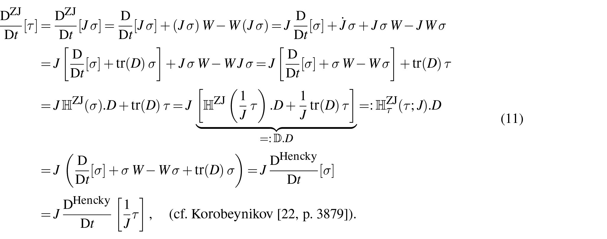
Proof. Starting with the Zaremba–Jaumann derivative of the Kirchhoff stress τ we obtain

$$\begin{array}{lll}\frac{{\mathrm{D}}^{\mathrm{ZJ}}}{\mathrm{D}t}[\tau ]\hfill & =\frac{\mathrm{D}}{\mathrm{D}t}[\tau ]+[\tau W-W\tau ]=\frac{\mathrm{D}}{\mathrm{D}t}[F{S}_2{F}^T]+[\tau W-W\tau ]\hfill & \hfill \\ \hfill & =\stackrel{.}{F}{S}_2{F}^T+F{\stackrel{.}{S}}_2{F}^T+F{S}_2{\stackrel{.}{F}}^T+[\tau W-W\tau ]\hfill & \hfill \\ \hfill & =F{\stackrel{.}{S}}_2{F}^T+\underset{L}{\underbrace{\stackrel{.}{F}{F}^{-1}}}\underset{\tau }{\underbrace{F{S}_2{F}^T}}+\underset{\tau }{\underbrace{F{S}_2{F}^T}}\underset{L^T}{\underbrace{F^{-T}{\stackrel{.}{F}}^T}}+[\tau W-W\tau ]\hfill & \hfill \\ \hfill & =F{\stackrel{.}{S}}_2{F}^T+L\tau +\tau L^T+\tau W-W\tau =F{\stackrel{.}{S}}_2{F}^T+D\tau +\tau D,L=D+W\hfill & \hfill \\ \hfill & =F{\mathrm{D}}_E{S}_2\left(E\right).[Ė]F^T+D\tau +\tau D\hfill & \hfill \\ \hfill & =F{\mathrm{D}}_E{S}_2\left(E\right).[F^{T}DF]F^T+D\tau +\tau D=:{ℍ}_{\tau }^{\mathrm{Z}\mathrm{J}}\left(\tau \right).D.\hfill \end{array}$$

(12)

In the second-last equation of (12) we used that by writing $S_2=S_2\left(E\right)$ with $E=\frac{1}{2}(F^{T}F-\mathbb{1})$ , we obtain ${\stackrel{.}{S}}_2\left(E\right)=D_E{S}_2\left(E\right).Ė,$ , where

$$Ė=\frac{1}{2}\left({\stackrel{.}{F}}^{T}F+F^T\stackrel{.}{F}\right)=\frac{1}{2}\left(F^T{F}^{-T}{\stackrel{.}{F}}^{T}F+F^T\stackrel{.}{F}{F}^{-1}F\right)=\frac{1}{2}\left(F^T{L}^{T}F+F^{T}LF\right)=F^{T}DF.$$

(13)

Since major symmetry of ${\mathbb{H}}_{\tau }^{\mathrm{ZJ}}\left(\tau \right)$ amounts to $〈{\mathbb{H}}_{\tau }^{\mathrm{ZJ}}\left(\tau \right).D_1,D_2〉=〈{\mathbb{H}}_{\tau }^{\mathrm{ZJ}}\left(\tau \right).D_2,D_1〉$ and the mapping $\mathrm{Sym}\left(3\right)\to \mathrm{Sym}\left(3\right),D\to \tau D+D\tau$ is already major symmetric, since with ${\tau }^T=\tau$

$$〈\tau D_1+D_1\tau ,D_2〉=〈D_1,{\tau }^T{D}_2+D_2{\tau }^T〉=〈D_1,\tau D_2+D_2\tau 〉.$$

(14)

It therefore remains to prove that the mapping $\mathrm{Sym}\left(3\right)\to \mathrm{Sym}\left(3\right),D\to F{\stackrel{·}{S}}_2{F}^T=F{\mathrm{D}}_E{S}_2\left(E\right).[F^{T}DF]$ is major symmetric, too. By assumption, the formulation is hyperelastic, which means that

$$S_2\left(E\right)={\mathrm{D}}_{E}W\left(E\right),$$

(15)

where W is the elastic energy. Thus it follows that ${\mathrm{D}}_E{S}_2\left(E\right)={\mathrm{D}}_E^{2}W\left(E\right)$ is itself self-adjoint, i.e., ${\left({\mathrm{D}}_E{S}_2\left(E\right)\right)}^T={\mathrm{D}}_E{S}_2\left(E\right)$ , meaning that

$$〈{\mathrm{D}}_E{S}_2\left(E\right).H_1,H_2〉=〈{\mathrm{D}}_E{S}_2\left(E\right).H_2,H_1〉\forall H_1,H_2\in \mathrm{Sym}\left(3\right).$$

(16)

Therefore, we obtain for the mapping $\mathrm{Sym}\left(3\right)\to \mathrm{Sym}\left(3\right),D\to F{D}_E{S}_2\left(E\right).[F^{T}DF]F^T$

$$\begin{array}{cc}\multicolumn{1}{c}{}& 〈F{\mathrm{D}}_E{S}_2\left(E\right).[F^T{D}_{1}F]F^T,D_2〉=〈{\mathrm{D}}_E{S}_2\left(E\right).[F^T{D}_{1}F],F^T{D}_{2}F〉\hfill \\ \multicolumn{1}{c}{}& =〈F^T{D}_{1}F,{\left({\mathrm{D}}_E{S}_2\left(E\right)\right)}^T.[F^T{D}_{2}F]〉\hfill \\ \multicolumn{1}{c}{}& =〈F^T{D}_{1}F,D_E{S}_2\left(E\right).[F^T{D}_{2}F]〉=〈D_1,F{D}_E{S}_2\left(E\right).[F^T{D}_{2}F]F^T〉,\hfill \end{array}$$

(17)

which is the required major symmetry. □

Remark 1.2. Minor symmetry of ${\mathbb{H}}_{\tau }^{\mathrm{ZJ}}\left(\tau \right)$ is clear from equation (12) since ${\mathbb{H}}_{\tau }^{\mathrm{ZJ}}\left(\tau \right).D\in \mathrm{Sym}\left(3\right),\forall D\in \mathrm{Sym}\left(3\right)$ . Moreover, minor and major symmetry of ${\mathbb{H}}_{\tau }^{\mathrm{ZJ}}\left(\tau \right)$ are independent of assuming isotropy.

Looking at equation $(\mathrm{11}{)}_3$ , it is clear that major symmetry of ${\mathbb{H}}_{\tau }^{\mathrm{ZJ}}\left(\tau \right)$ does not imply that ${\mathbb{H}}^{\mathrm{ZJ}}\left(\sigma \right)$ is major symmetric, apart from the incompressible case in which $\mathrm{tr}\left(D\right)=0$ .

We observe that in the incompressible case, we have $J=1$ and $\mathrm{tr}\left(D\right)=0$ and therefore

$${\mathbb{H}}_{\tau }^{\mathrm{ZJ}}(\tau ;1)={\mathbb{H}}^{\mathrm{ZJ}}\left(\tau \right)\mathrm{together}\mathrm{with}\frac{{\mathrm{D}}^{\mathrm{ZJ}}}{\mathrm{D}t}[\tau ]={\mathbb{H}}^{\mathrm{ZJ}}\left(\tau \right).D$$

(18)

so that the latter rate formulation for τ coincides with the Cauchy stress rate-formulation, as it should be for the incompressible case in which $\sigma =\tau$ .

There is also a more direct way to obtain the rate-formulation in terms of the Zaremba–Jaumann rate and the Kirchhoff stress τ in the case of isotropy. Indeed, for isotropy, the Kirchhoff stress satisfies

$$Q\tau \left(B\right)Q^T=\tau \left(QB{Q}^T\right)\forall Q\in O\left(3\right).$$

(19)

Therefore, we obtain (cf. Neff et al. [24, 26])

$$\begin{array}{lll}\frac{{\mathrm{D}}^{\mathrm{ZJ}}}{\mathrm{D}t}[\tau ]=D_B\tau \left(B\right).[BD+DB]\hfill & =:{ℍ}_{\tau }^{\mathrm{Z}\mathrm{J}}\left(\tau \right).DifB\mapsto \tau \left(B\right)\mathrm{is}\mathrm{invertible}\hfill & \hfill \\ \hfill & =J\mathbb{D}\left(\tau \right).D(\mathrm{Abaqus}\mathrm{™}-\mathrm{format}).\hfill & \hfill \end{array}$$

(20)

According to the Abaqus™ user manual, for three-dimensional (3D) continuum elements Abaqus™ uses the elasticity tensor associated with the Zaremba–Jaumann rate for the Kirchhoff stress τ, i.e., the positive definiteness of ${\mathbb{H}}_{\tau }^{\mathrm{ZJ}}$ (i.e. $\mathbb{D}\left(\tau \right)$ ) is checked for material stability.

1.3. Alternative approach and absolute expression of ${\mathbb{H}}_{\tau }^{\mathrm{ZJ}}\left(\tau \right)$

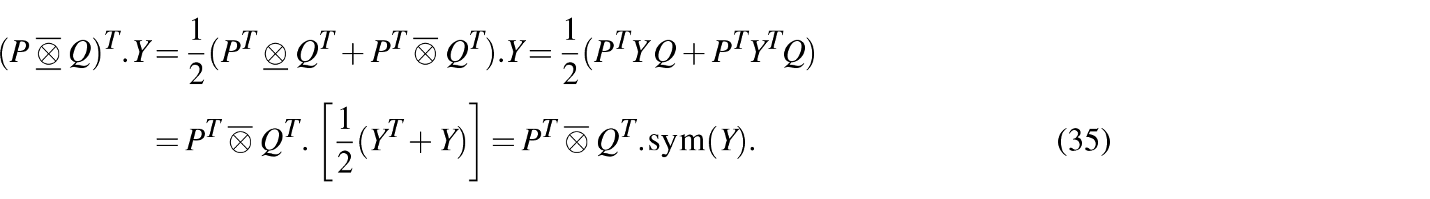
An absolute expression of the Zaremba–Jaumann elasticity tensor ${\mathbb{H}}_{\tau }^{\mathrm{ZJ}}\left(\tau \right)$ , i.e., an expression not involving the double contraction with the deformation rate D, can be obtained using the special tensor products $\underset{¯}{\mathrm{\otimes }}$ and $\overline{\mathrm{\otimes }}$ and, specifically, their symmetrisation $\overline{\underset{¯}{\otimes }}$ , as defined in the work by Curnier et al. [31]. We shall define these tensors for the case of Cartesian coordinates, but general covariant expressions can be found in studies by Bellini and Federico [16], Federico and Grillo [32] and Federico [33]. As in the remainder of this work, $\mathbb{T}.Z$ means that the fourth-order tensor $\mathbb{T}$ acts as a linear map on the second-order tensor Z. The transpose of the fourth-order tensor $\mathbb{T}$ is defined as the tensor ${\mathbb{T}}^T$ such that, for every second-order tensors Y and Z,

$$〈Y,\mathbb{T}.Z〉=〈Z,{\mathbb{T}}^T.Y〉,Y_{\mathrm{ij}}{\mathbb{T}}_{\mathrm{ijkl}}{Z}_{\mathrm{kl}}=Z_{\mathrm{kl}}{\left({\mathbb{T}}^T\right)}_{\mathrm{klij}}{Y}_{\mathrm{ij}}.$$

(21)

In the literature on the special tensor products $\underset{¯}{\otimes }$ and $\overline{\mathrm{\otimes }}$ [16, 17, 31–35], the action $\mathbb{T}.Z$ of $\mathbb{T}$ on Z is usually denoted with the double contraction symbol, i.e., the colon “:”, as $\mathbb{T}:Z$ . In the same literature, the colon “:” is also used for the double contraction of two second-order tensors, $Y:Z$ , which here is denoted by the scalar product $〈Y,Z〉$ .

1.3.1. Standard and special tensor products

The standard tensor product ⊗ maps two second-order tensors P and Q into the fourth-order tensor $P\otimes Q$ , defined by

$$\begin{array}{cc}\left(P\otimes Q\right).Z=〈Q,Z〉P& {\left(P\otimes Q\right)}_{ijkl}{Z}_{kl}=\left(Q_{kl}{Z}_{kl}\right)P_{ij},\end{array}$$

(22)

for every second-order tensor Z. Therefore, the component expression of $P\otimes Q$ is the familiar

$${(P\otimes Q)}_{\mathrm{ijkl}}=P_{\mathrm{ij}}{Q}_{\mathrm{kl}}{P}_{\mathrm{ij}}.$$

(23)

It is easy to verify, in components or with the definition (22) of tensor product and the definition (21) of transpose of a fourth-order tensor, that

$${(P\otimes Q)}^T=Q\otimes P.$$

(24)

Indeed, using, e.g., equations (22) and (21), we have

$$\begin{array}{c}\multicolumn{1}{c}{〈Y,(P\otimes Q).Z〉=〈Y,〈Q,Z〉P〉=〈Y,P〉〈Q,Z〉=〈Z,Q〉〈P,Y〉}\\ \multicolumn{1}{c}{=〈Z,〈P,Y〉Q〉=〈Z,(Q\otimes P)Y〉=〈Z,{(P\otimes Q)}^{T}Y〉,}\end{array}$$

(25)

which, for the arbitrariness of Y and Z, implies equation (24).

The special tensor product $\underset{¯}{\otimes }$ (denoted ⊠ by some authors, e.g., Korobeynikov [21, 22], Del Piero [36], Lucchesi [37], and Jog [38]) maps two second-order tensors P and Q into the fourth-order tensor $P\underset{¯}{\otimes }Q$ defined by

$$\begin{array}{cc}\left(P\underset{¯}{\otimes }Q\right).Z=PZ{Q}^T& {\left(P\underset{¯}{\otimes }Q\right)}_{ijkl}{Z}_{kl}=P_{ik}{Z}_{kl}{Q}_{jl},\end{array}$$

(26)

for every second-order tensor Z. The component expression of $P\underset{¯}{\otimes }Q$ is thus

$${\left(P\underset{¯}{\otimes }Q\right)}_{\mathrm{ijkl}}=P_{\mathrm{ik}}{Q}_{\mathrm{jl}}.$$

(27)

For the case of the special tensor product $\underset{¯}{\otimes }$ , the transpose is

$${\left(P\underset{¯}{\otimes }Q\right)}^T=P^T\underset{¯}{\otimes }{Q}^T,$$

(28)

which can be verified in components or by the definition (26) of $\underset{¯}{\otimes }$ and the general definition (21) of transpose of a fourth-order tensor.

The special tensor product $\overline{\mathrm{\otimes }}$ maps two second-order tensors P and Q into the fourth-order tensor $P\overline{\otimes }Q$ defined by

$$\begin{array}{cc}\left(P\overline{\otimes }Q\right).Z=P{Z}^T{Q}^T,& {\left(P\overline{\otimes }Q\right)}_{ijkl}{Z}_{kl}=P_{il}{Z}_{kl}{Q}_{jk},\end{array}$$

(29)

for every second-order tensor Z. The component expression of $P\overline{\otimes }Q$ is thus

$${\left(P\overline{\otimes }Q\right)}_{\mathrm{ijkl}}=P_{\mathrm{il}}{Q}_{\mathrm{jk}}.$$

(30)

For the case of the special tensor product $\overline{\mathrm{\otimes }}$ , the transpose is

$${\left(P\overline{\otimes }Q\right)}^T=Q^T\overline{\otimes }{P}^T,$$

(31)

which, again, can be verified in components or by the definition (29) of $\overline{\mathrm{\otimes }}$ and the general definition (21).

1.3.2. Symmetrisation of the special tensor products

In general, the special tensor products $\underset{¯}{\otimes }$ and $\overline{\mathrm{\otimes }}$ possess neither the major symmetry nor the minor symmetries. However, symmetrisations exist that turn out to be very useful.

The tensor product $\underset{¯}{\overline{\otimes }}$ (denoted ⊙ by some authors, e.g., Holzapfel [39]) is defined by

$$\begin{array}{cc}P\underset{¯}{\overline{\otimes }}Q=\frac{1}{2}\left(P\underset{¯}{\otimes }Q+Q\overline{\otimes }P\right),& {(P\underset{¯}{\overline{\otimes }}Q)}_{ijkl}=\frac{1}{2}\left(P_{ik}{Q}_{jl}+Q_{il}{P}_{jk}\right).\end{array}$$

(32)

The transpose of the fourth-order $P\underset{¯}{\overline{\otimes }}Q$ is not obtainable via $\underset{¯}{\overline{\otimes }}$ . Indeed, using equations (28) and (31), we have

$${\left(P\underset{¯}{\overline{\otimes }}Q\right)}^T=\frac{1}{2}(P^T\underset{¯}{\otimes }{Q}^T+P^T\overline{\otimes }{Q}^T).$$

(33)

The tensor $P\underset{¯}{\overline{\otimes }}Q$ possesses the left minor symmetry [16], i.e., the minor symmetry on the first pair of indices. This can be verified easily in components, or by studying the action of $P\underset{¯}{\overline{\otimes }}Q$ on an arbitrary second-order tensor Z:

$$\begin{array}{c}\multicolumn{1}{c}{\left(P\underset{¯}{\overline{\otimes }}Q\right).Z=\frac{1}{2}(PZ{Q}^T+Q{Z}^T{P}^T)=\frac{1}{2}(PZ{Q}^T+{\left(PZ{Q}^T\right)}^T)=\mathrm{sym}\left(PZ{Q}^T\right)}\\ \multicolumn{1}{c}{=\mathrm{sym}[\left(P\underset{¯}{\otimes }Q\right).Z].}\end{array}$$

(34)

In contrast, $P\underset{¯}{\overline{\otimes }}Q$ does not possess the right minor symmetry and, again, this can be verified in components, or by studying the action of its transpose ${\left(P\underset{¯}{\overline{\otimes }}Q\right)}^T$ on an arbitrary second-order tensor Y:

$$\begin{array}{c}\multicolumn{1}{c}{{\left(P\underset{¯}{\overline{\otimes }}Q\right)}^T.Y=\frac{1}{2}(P^T\underset{¯}{\otimes }{Q}^T+P^T\overline{\otimes }{Q}^T).Y=\frac{1}{2}(P^{T}YQ+P^T{Y}^{T}Q)}\\ \multicolumn{1}{c}{=P^T\overline{\otimes }{Q}^T.\left[\frac{1}{2}(Y^T+Y)\right]=P^T\overline{\otimes }{Q}^T.\mathrm{sym}\left(Y\right).}\end{array}$$

(35)

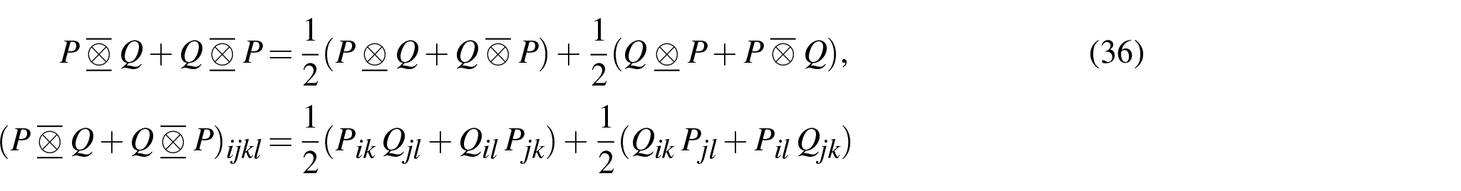
The further symmetrisation

$$\begin{array}{c}\multicolumn{1}{c}{P\underset{¯}{\overline{\otimes }}Q+Q\underset{¯}{\overline{\otimes }}P=\frac{1}{2}(P\underset{¯}{\otimes }Q+Q\overline{\otimes }P)+\frac{1}{2}(Q\underset{¯}{\otimes }P+P\overline{\otimes }Q),}\\ \multicolumn{1}{c}{{(P\underset{¯}{\overline{\otimes }}Q+Q\underset{¯}{\overline{\otimes }}P)}_{\mathrm{ijkl}}=\frac{1}{2}(P_{\mathrm{ik}}{Q}_{\mathrm{jl}}+Q_{\mathrm{il}}{P}_{\mathrm{jk}})+\frac{1}{2}(Q_{\mathrm{ik}}{P}_{\mathrm{jl}}+P_{\mathrm{il}}{Q}_{\mathrm{jk}})}\end{array}$$

(36)

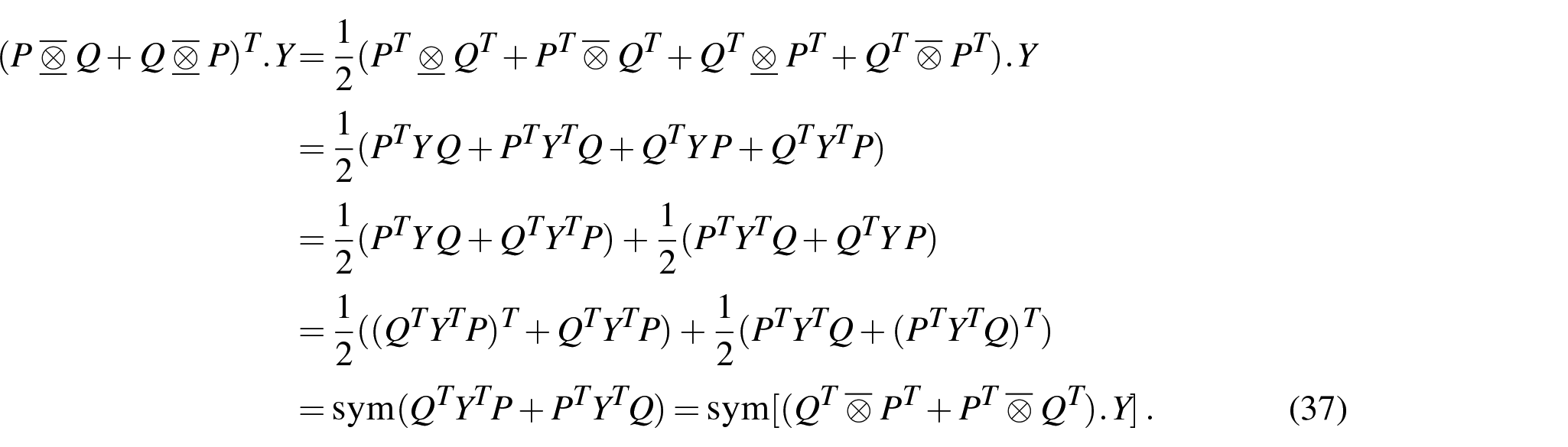
possesses both minor symmetries. Indeed, the left minor symmetry follows from the fact that each of $P\underset{¯}{\overline{\otimes }}Q$ and $Q\underset{¯}{\overline{\otimes }}P$ possesses the minor symmetry, by virtue of equation (34), and the right minor symmetry can be verified easily in components or, as above, by studying the action of the transpose ${(P\underset{¯}{\overline{\otimes }}Q+Q\underset{¯}{\overline{\otimes }}P)}^T$ , which is easily obtainable from equation (33), on an arbitrary second-order tensor Y:

$$\begin{array}{c}\multicolumn{1}{c}{{(P\underset{¯}{\overline{\otimes }}Q+Q\underset{¯}{\overline{\otimes }}P)}^T.Y=\frac{1}{2}(P^T\underset{¯}{\otimes }{Q}^T+P^T\overline{\otimes }{Q}^T+Q^T\underset{¯}{\otimes }{P}^T+Q^T\overline{\otimes }{P}^T).Y}\\ \multicolumn{1}{c}{=\frac{1}{2}(P^{T}YQ+P^T{Y}^{T}Q+Q^{T}YP+Q^T{Y}^{T}P)}\\ \multicolumn{1}{c}{=\frac{1}{2}(P^{T}YQ+Q^T{Y}^{T}P)+\frac{1}{2}(P^T{Y}^{T}Q+Q^{T}YP)}\\ \multicolumn{1}{c}{=\frac{1}{2}({\left(Q^T{Y}^{T}P\right)}^T+Q^T{Y}^{T}P)+\frac{1}{2}(P^T{Y}^{T}Q+{\left(P^T{Y}^{T}Q\right)}^T)}\\ \multicolumn{1}{c}{=\mathrm{sym}(Q^T{Y}^{T}P+P^T{Y}^{T}Q)=\mathrm{sym}[(Q^T\overline{\otimes }{P}^T+P^T\overline{\otimes }{Q}^T).Y].}\end{array}$$

(37)

Finally, if both P and Q are symmetric, then $P\underset{¯}{\overline{\otimes }}Q+Q\underset{¯}{\overline{\otimes }}P$ also possesses the major symmetry, i.e., for every second-order tensors Y and Z,

$$〈Y,(P\underset{¯}{\overline{\otimes }}Q+Q\underset{¯}{\overline{\otimes }}P).Z〉=〈Z,(P\underset{¯}{\overline{\otimes }}Q+Q\underset{¯}{\overline{\otimes }}P).Y〉.$$

(38)

As usual, this can be verified in components, or by working out the (double) contractions.

1.3.3. Lie derivative of the Kirchhoff stress and spatial elasticity tensor

The Lie derivative of the Kirchhoff stress τ is related directly to the material elasticity tensor

$$\mathbb{C}:=D_E{S}_2\left(E\right)$$

(39)

as already seen in equation (12). Indeed, the material elasticity tensor (39) features in the rate expression of the second Piola–Kirchhoff stress,

$${\stackrel{.}{S}}_2=D_E{S}_2\left(E\right).Ė=\mathbb{C}.Ė$$

(40)

and, since the second Piola–Kirchhoff stress $S_2$ is the pull-back of the Kirchhoff stress τ, i.e.,

$$S_2=F^{-1}\tau F^{-T},$$

(41)

the push-forward of the time derivative (40) of $S_2$ is, by definition, the Lie derivative of the Kirchhoff stress τ, as per equation (100). Therefore,

$$\begin{array}{l}{ℒ}_v\tau =F\left[\frac{\mathrm{D}}{\mathrm{D}t}[F^{-1}\tau F^{-T}]\right]F^T=F{\stackrel{.}{S}}_2{F}^T=F[\mathbb{C}.Ė]F^T.\hfill \end{array}$$

(42)

We aim at expressing the Lie derivative (42) as a function of the spatial elasticity tensor,

$$\mathbb{C}=J^{-1}\left(F\underset{¯}{\otimes }F\right).[\mathbb{C}.\left(F^T\underset{¯}{\otimes }{F}^T\right)],{\mathbb{C}}_{\mathrm{ijkl}}=J^{-1}{F}_{\mathrm{iI}}{F}_{\mathrm{jJ}}{\mathbb{C}}_{\mathrm{IJKL}}{F}_{\mathrm{kK}}{F}_{\mathrm{lL}},$$

(43)

which is the full backward Piola transform of the material elasticity tensor $\mathbb{C}$ , and relates the Truesdell rate (cf. Appendix 1) of the Cauchy stress σ to the deformation rate D [8, 14, 32, 33]. Note how the use of the special tensor product $\underset{¯}{\otimes }$ allows to write the backward Piola transformation equation (43) in component-free formalism, via the tensor $F\underset{¯}{\otimes }F$ and its transpose ${\left(F\underset{¯}{\otimes }F\right)}^T=F^T\underset{¯}{\otimes }{F}^T$ [33, 40]. The inverse relation of equation (43) is

$$\mathbb{C}=J\left(F^{-1}\underset{¯}{\otimes }{F}^{-1}\right).[\mathbb{C}.\left(F^{-T}\underset{¯}{\otimes }{F}^{-T}\right)],{\mathbb{C}}_{\mathrm{IJKL}}=J{F}_{\mathrm{Ii}}^{-1}{F}_{\mathrm{Jj}}^{-1}{\mathbb{C}}_{\mathrm{ijkl}}{F}_{\mathrm{Kk}}^{-1}{F}_{\mathrm{Ll}}^{-1}.$$

(44)

It is easy to show (for instance, in components), that substitution of equation (44) into equation (42) yields

$${\mathcal{L}}_v\tau =J\mathbb{C}.D,$$

(45)

where we exploited the fact that the rate of deformation D is the push-forward of the time derivative E:

$$D=F^{-T}ĖF^{-1}.$$

(46)

1.3.4. Zaremba–Jaumann rate of the Kirchhoff stress and its conjugated elasticity tensor

Here, we use the Cartesian expressions of some results from Appendix 1, which were obtained in covariant formalism. Substitution of the expression (45) of the Lie derivative of τ into the Zaremba–Jaumann rate (118) of τ yields

$$\frac{{\mathrm{D}}^{\mathrm{ZJ}}}{\mathrm{D}t}[\tau ]=J\mathbb{C}.D+D\tau +\tau D.$$

(47)

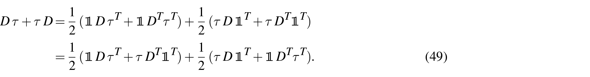
In order to find an absolute expression of the elasticity tensor ${\mathbb{H}}_{\tau }^{\mathrm{ZJ}}\left(\tau \right)$ relating the Zaremba–Jaumann rate of τ to the deformation rate D, we need to express the term $D\tau +\tau D$ as a fourth-order tensor double-contracted with D. We note that, by definition of identity tensor $\mathbb{1}$ (which, in this case, means the spatial identity tensor and, rigorously speaking, would be the inverse metric tensor $g^{-1}$ , which has contravariant components $g^{\mathrm{ij}}$ , similarly to the Kirchhoff stress τ, which has contravariant components ${\tau }^{\mathrm{ij}}$ ), we have the identity

$$D\tau +\tau D=\mathbb{1}D\tau +\tau D\mathbb{1}.$$

(48)

By virtue of the symmetry all the tensors involved, i.e., ${\mathbb{1}}^T=\mathbb{1}$ , $D^T=D$ , ${\tau }^T=\tau$ , this can be written

$$\begin{array}{c}\multicolumn{1}{c}{D\tau +\tau D=\frac{1}{2}(\mathbb{1}D{\tau }^T+\mathbb{1}{D}^T{\tau }^T)+\frac{1}{2}(\tau D{\mathbb{1}}^T+\tau D^T{\mathbb{1}}^T)}\\ \multicolumn{1}{c}{=\frac{1}{2}(\mathbb{1}D{\tau }^T+\tau D^T{\mathbb{1}}^T)+\frac{1}{2}(\tau D{\mathbb{1}}^T+\mathbb{1}{D}^T{\tau }^T).}\end{array}$$

(49)

In equation (49), we recognise the symmetrised special tensor product $\mathbb{1}\underset{¯}{\overline{\otimes }}\tau +\tau \underset{¯}{\overline{\otimes }}\mathbb{1}$ defined in equation (36), i.e., we can write equation (49) as

$$D\tau +\tau D=[\mathbb{1}\underset{¯}{\overline{\otimes }}\tau +\tau \underset{¯}{\overline{\otimes }}\mathbb{1}].D.$$

(50)

Substitution of equation (50) into equation (47) yields

$$\frac{{\mathrm{D}}^{\mathrm{ZJ}}}{\mathrm{D}t}[\tau ]=[J\mathbb{C}+\mathbb{1}\underset{¯}{\overline{\otimes }}\tau +\tau \underset{¯}{\overline{\otimes }}\mathbb{1}].D,$$

(51)

which compared with equation (12), finally gives the sought absolute expression of ${\mathbb{H}}_{\tau }^{\mathrm{ZJ}}\left(\tau \right)$ , as

$${\mathbb{H}}_{\tau }^{\mathrm{ZJ}}\left(\tau \right)=J\mathbb{C}+\mathbb{1}\underset{¯}{\overline{\otimes }}\tau +\tau \underset{¯}{\overline{\otimes }}\mathbb{1},$$

(52)

or, in components:

$$[{\mathbb{H}}_{\tau }^{\mathrm{ZJ}}\left(\tau \right){]}_{\mathrm{ijkl}}=J{\mathbb{C}}_{\mathrm{ijkl}}+\frac{1}{2}({\delta }_{\mathrm{ik}}{\tau }_{\mathrm{jl}}+{\tau }_{\mathrm{il}}{\delta }_{\mathrm{jk}})+\frac{1}{2}({\tau }_{\mathrm{ik}}{\delta }_{\mathrm{jl}}+{\delta }_{\mathrm{il}}{\tau }_{\mathrm{jk}}).$$

(53)

The elasticity tensor ${\mathbb{H}}_{\tau }^{\mathrm{ZJ}}\left(\tau \right)$ defined in equation (52) possesses the major symmetry and both minor symmetries, which follow from those of $\mathbb{C}$ and $\mathbb{1}\underset{¯}{\overline{\otimes }}\tau +\tau \underset{¯}{\overline{\otimes }}\mathbb{1}$ (the major symmetry of $\mathbb{1}\underset{¯}{\overline{\otimes }}\tau +\tau \underset{¯}{\overline{\otimes }}\mathbb{1}$ descends from the symmetry of τ and $\mathbb{1}$ ).

The spatial elasticity tensor $\mathbb{C}$ inherits the major symmetry and both minor symmetries from the material elasticity tensor $\mathbb{C}$ , which, in turn, enjoys the major symmetry because of the smoothness of the elastic potential (Schwarz’ theorem on the symmetry of the second partial derivatives), and both minor symmetries because of the symmetry of the Green-Lagrange strain E. The symmetrised special tensor product $\mathbb{1}\underset{¯}{\overline{\otimes }}\tau +\tau \underset{¯}{\overline{\otimes }}\mathbb{1}$ possesses both minor symmetries, as shown in equations (34) and (37), and, by virtue of the symmetry of τ and 1, it also possesses the major symmetry, as shown in equation (38). In a past work Palizi et al. [17], the major symmetry was missed because, in place of the symmetrised contribution $\mathbb{1}\underset{¯}{\overline{\otimes }}\tau +\tau \underset{¯}{\overline{\otimes }}\mathbb{1}$ , the contribution $\tau \underset{¯}{\otimes }\mathbb{1}+\mathbb{1}\overline{\otimes }\tau =2\left(\tau \underset{¯}{\overline{\otimes }}\mathbb{1}\right)$ was used. This was the result of not accounting explicitly for the symmetry of τ and 1.

We remark that the component expression (53) is particularly convenient for the numerical implementation of ${\mathbb{H}}_{\tau }^{\mathrm{ZJ}}\left(\tau \right)$ , regardless of the specific software package at hand. As mentioned in Section 1.2, the programming of Abaqus™ UMAT user-defined material subroutines requires the elasticity tensor

$$\mathbb{D}\left(\tau \right)=J^{-1}{\mathbb{H}}_{\tau }^{\mathrm{ZJ}}\left(\tau \right)=\mathbb{C}+J^{-1}(\mathbb{1}\underset{¯}{\overline{\otimes }}\tau +\tau \underset{¯}{\overline{\otimes }}\mathbb{1}).$$

(54)

Last, we note again that, in covariant formalism, the identity 1 must be replaced by the inverse metric tensor $g^{-1}$ .

1.3.5. Truesdell rate of the Cauchy stress and spatial elasticity tensor

Similarly to the case of the Lie derivative of the Kirchhoff stress τ, the Truesdell rate of the Cauchy stress is related directly to the material elasticity tensor $\mathbb{C}$ of equation (39). Indeed, the second Piola–Kirchhoff stress $S_2$ is the backward Piola transform of the Cauchy stress σ, i.e.,

$$S_2=J{F}^{-1}\sigma F^{-T},$$

(55)

and the forward Piola transform of the time derivative (40) of $S_2$ is, by definition, the Truesdell rate of the Cauchy stress σ, as per equation (116). Therefore,

$$\frac{D^{TR}}{\mathrm{D}t}[\sigma ]=J^{-1}F\left[\frac{\mathrm{D}}{\mathrm{D}t}[J{F}^{-1}\sigma F^{-T}]\right]F^T=J^{-1}F{\stackrel{.}{S}}_2{F}^T=J^{-1}F[\mathbb{C}.Ė]F^T.$$

(56)

With the same procedure seen above for the Lie derivative ${\mathcal{L}}_v\tau$ of the Kirchhoff stress τ, we can show that the Truesdell rate equation (56) of the Cauchy stress σ is related to the spatial elasticity tensor $\mathbb{C}$ of equation (43) via

$$\frac{{\mathrm{D}}^{\mathrm{TR}}}{\mathrm{D}t}[\sigma ]=\mathbb{C}.D.$$

(57)

1.3.6. Zaremba–Jaumann rate of the Cauchy stress and its conjugated elasticity tensor

We refer again to Appendix 1. Substitution of the expression (57) of the Truesdell rate of σ into the Zaremba–Jaumann rate equation (119) of σ yields

$$\frac{{\mathrm{D}}^{\mathrm{ZJ}}}{\mathrm{D}t}[\sigma ]=\mathbb{C}.D+D\sigma +\sigma D-\mathrm{tr}\left(D\right)\sigma .$$

(58)

The term $D\sigma +\sigma D$ is obtained by simply dividing equation (50) by J, as

$$D\sigma +\sigma D=[\mathbb{1}\underset{¯}{\overline{\otimes }}\sigma +\sigma \underset{¯}{\overline{\otimes }}\mathbb{1}].D,$$

(59)

and the term $\mathrm{tr}\left(D\right)\sigma$ is obtained via the definitions of the trace and (standard) tensor product, as

$$\mathrm{tr}\left(D\right)\sigma =〈\mathbb{1},D〉\sigma =(\sigma \otimes \mathbb{1}).D.$$

(60)

Substitution of equations (59) and (60) into equation (58) yields

$$\frac{{\mathrm{D}}^{\mathrm{ZJ}}}{\mathrm{D}t}[\sigma ]=[\mathbb{C}+\mathbb{1}\underset{¯}{\overline{\otimes }}\sigma +\sigma \underset{¯}{\overline{\otimes }}\mathbb{1}-(\sigma \otimes \mathbb{1})].D,$$

(61)

which, compared with equations (5) and (65) yields the absolute expression of ${\mathbb{H}}^{\mathrm{ZJ}}\left(\sigma \right)$ as

$${\mathbb{H}}^{\mathrm{ZJ}}\left(\sigma \right)=\mathbb{C}+\mathbb{1}\underset{¯}{\overline{\otimes }}\sigma +\sigma \underset{¯}{\overline{\otimes }}\mathbb{1}-\sigma \otimes \mathbb{1},$$

(62)

or, in components,

$$[{\mathbb{H}}^{\mathrm{ZJ}}\left(\sigma \right){]}_{\mathrm{ijkl}}={\mathbb{C}}_{\mathrm{ijkl}}+\frac{1}{2}({\delta }_{\mathrm{ik}}{\sigma }_{\mathrm{jl}}+{\sigma }_{\mathrm{il}}{\delta }_{\mathrm{jk}})+\frac{1}{2}({\sigma }_{\mathrm{ik}}{\delta }_{\mathrm{jl}}+{\delta }_{\mathrm{il}}{\sigma }_{\mathrm{jk}})-{\sigma }_{\mathrm{ij}}{\delta }_{\mathrm{kl}}.$$

(63)

All considerations made for ${\mathbb{H}}_{\tau }^{\mathrm{ZJ}}\left(\tau \right)$ hold for ${\mathbb{H}}_{\sigma }^{\mathrm{ZJ}}\left(\sigma \right)$ , except for the fact that ${\mathbb{H}}_{\sigma }^{\mathrm{ZJ}}\left(\sigma \right)$ does not posses major symmetry, due to the presence of the term $\sigma \otimes \mathbb{1}$ which can only be major symmetric when the Cauchy stress σ is hydrostatic: not a very interesting scenario, and certainly not a general scenario. Finally, we note again that, in covariant formalism, the identity 1 must be replaced by the inverse metric tensor $g^{-1}$ .

As for the relevance of the representation equation (63), we observe that indeed, in the works by by Li and Wang [41, equation (6)], by Wang et al. [42, equation (2.22)], and by Morris and Krenn [43, equation (22)], the following (largely ad hoc) constitutive stiffness tensor is analysed for stability of the elastic law,

$${\mathbb{H}}_{\mathrm{ijkl}}\left(\sigma \right)={\mathbb{C}}_{\mathrm{ijkl}}+\frac{1}{2}({\delta }_{\mathrm{ik}}{\sigma }_{\mathrm{jl}}+{\sigma }_{\mathrm{il}}{\delta }_{\mathrm{jk}}+{\sigma }_{\mathrm{ik}}{\delta }_{\mathrm{jl}}+{\delta }_{\mathrm{il}}{\sigma }_{\mathrm{jk}}-2{\delta }_{\mathrm{kl}}{\sigma }_{\mathrm{ij}}),$$

(64)

where $\mathbb{C}$ is interpreted by us as the spatial elasticity tensor occurring in equation (57) ([42, equation (2.22)]) and the authors define [material] instability to be present at $\mathbb{H}\left(\sigma \right)=0$ . Taking into account equation (63), it occurs therefore that the above ${\mathbb{H}}_{\mathrm{ijkl}}$ coincides with the induced tangent stiffness matrix appearing in the rate-formulation for the Cauchy stress σ and the Zaremba–Jaumann rate [26]

$$\begin{array}{cc}\frac{{\mathrm{D}}^{\mathrm{ZJ}}}{\mathrm{D}t}[\sigma ]={\mathbb{H}}^{\mathrm{Z}\mathrm{J}}\left(\sigma \right).D,& {\mathbb{H}}^{\mathrm{ZJ}}\left(\sigma \right).D:={\mathrm{D}}_B\sigma \left(B\right).[BD+DB].\end{array}$$

(65)

The condition ${\mathbb{H}}^{\mathrm{ZJ}}\left(\sigma \right)=0$ is, in fact, equivalent to checking (cf. Neff et al. [26]) the local invertibility of $B\to \sigma \left(B\right)$ , i.e.

$$det{\mathrm{D}}_B\sigma \left(B\right)=0.$$

(66)

In the paper [42], the authors check, in this interpretation,

$$det\left(\mathrm{sym}{\mathbb{H}}^{\mathrm{ZJ}}\left(\sigma \right)\right)=0$$

(67)

being aware that ${\mathbb{H}}^{\mathrm{ZJ}}\left(\sigma \right)$ is, in general, not major symmetric and we note that [25, 44, 45]

$$〈\mathrm{sym}{\mathbb{H}}^{\mathrm{ZJ}}\left(\sigma \right).D,D〉>0\iff {\mathrm{D}}_{\log V}\sigma \left(\log V\right)\in {\mathrm{Sym}}_4^{++}\left(6\right)\stackrel{(\mathrm{Def})}{\iff }\mathrm{TSTS}-{\mathrm{M}}^{++}.$$

(68)

Moreover by the Bendixson Theorem [46], equation (68) implies ${\mathbb{H}}^{\mathrm{ZJ}}\left(\sigma \right)>0$ , hence excluding equation (66).

2. The induced tangent stiffness tensor ${\mathbb{H}}_{\tau }^{\mathrm{ZJ}}\left(\tau \right)$ for the Hencky energy

2.1. The compressible Hencky energy

Let us now present as an example of the foregoing development the Hencky model. The Hencky energy (see Neff et al. [47–49] and Xiao et al. [12, 13, 50, 51] for related literature) reads

$${\mathrm{W}}_{\mathrm{Hencky}}\left(V\right)={\hat{\mathrm{W}}}_{\mathrm{Hencky}}\left(\log V\right)=\mu \Vert \log V{\Vert }^2+\frac{\mathrm{\lambda }}{2}\mathrm{t}{\mathrm{r}}^2\left(\log V\right)=\frac{\mu }{2}\Vert \log B{\Vert }^2+\frac{\mathrm{\lambda }}{4}{(\log detB)}^2.$$

(69)

The corresponding Kirchhoff stress τ can be calculated using the Richter representation [52–59]

$$\tau ={\mathrm{D}}_{\log V}\hat{\mathrm{W}}\left(\log V\right)=2\mu \log V+\mathrm{\lambda }\mathrm{tr}\left(\log V\right)1=\mu B+\frac{\mathrm{\lambda }}{2}\mathrm{tr}\left(\log B\right)\mathbb{1}.$$

(70)

For $\mu ,2\mu +3\mathrm{\lambda }>0$ , Hill’s inequality is satisfied (cf. Hill [60–62] and Sidoroff [63])

$$〈\tau \left(\log V_1\right)-\tau \left(\log V_2\right),\log V_1-\log V_2〉>0\forall V_1,V_2\in \mathrm{Sy}{\mathrm{m}}^{++}\left(3\right),V_1\ne V_2$$

(71)

and we even have

$${\mathrm{D}}_{\log V}\tau \left(\log V\right)={\mathrm{D}}_{\log V}^2{\hat{\mathrm{W}}}_{\mathrm{Hencky}}\left(\log V\right)\in {\mathrm{Sym}}_4^{++}\left(6\right),$$

(72)

since

$$〈{\mathrm{D}}_{\log V}\tau \left(\log V\right).H,H〉=〈2\mu H+\mathrm{\lambda }\mathrm{tr}\left(H\right)\mathbb{1},H〉=2\mu \parallel H{\parallel }^2+\mathrm{\lambda }\mathrm{t}{\mathrm{r}}^2\left(H\right)>0$$

(73)

and ${\hat{\mathrm{W}}}_{\mathrm{Hencky}}\left(\log V\right)$ is convex in $\log V$ .

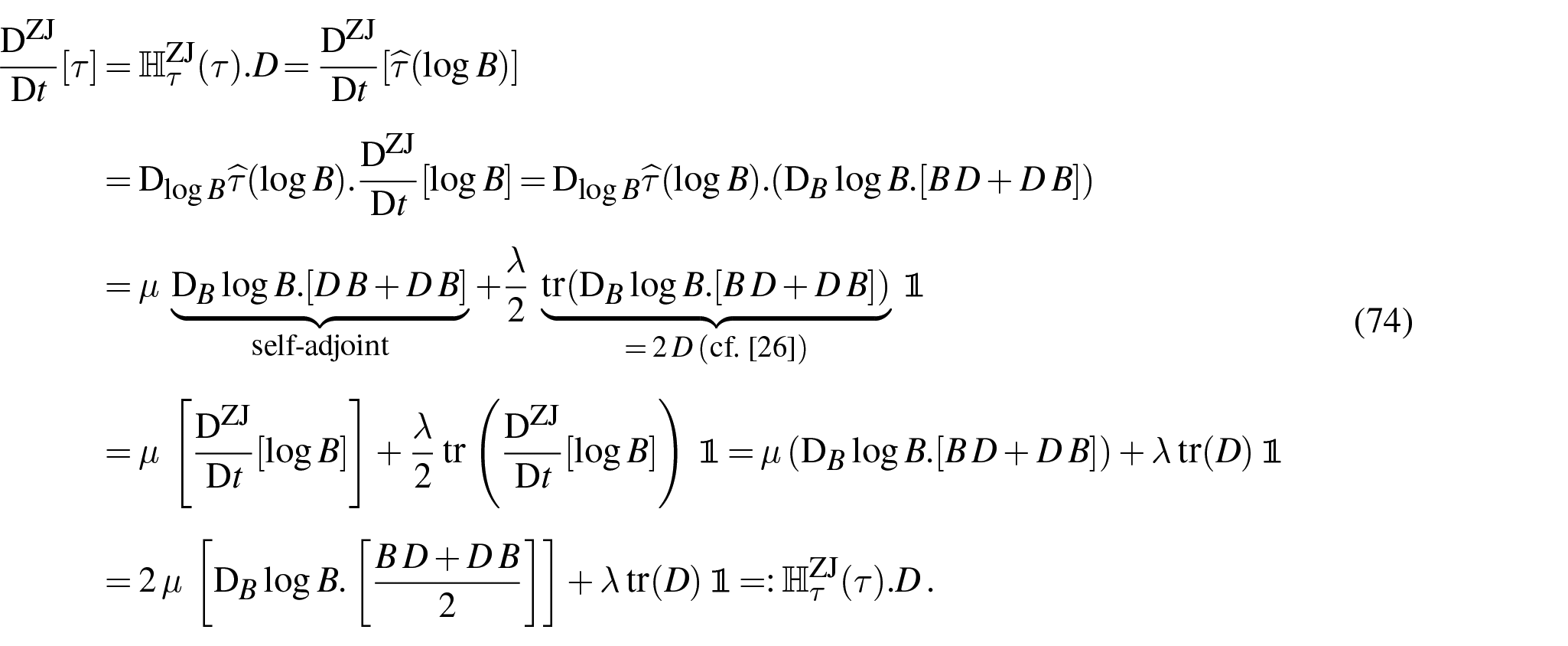
We wish to directly determine the rate-formulation for the Kirchhoff stress τ with the Zaremba–Jaumann rate. From d’Agostino et al. [44] and Neff et al. [24, 26], we have

$$\begin{array}{c}\multicolumn{1}{c}{}\\ \multicolumn{1}{c}{\frac{{\mathrm{D}}^{\mathrm{ZJ}}}{\mathrm{D}t}[\tau ]={\mathbb{H}}_{\tau }^{\mathrm{ZJ}}\left(\tau \right).D=\frac{{\mathrm{D}}^{\mathrm{ZJ}}}{\mathrm{D}t}[\hat{\tau }\left(\log B\right)]}\\ \multicolumn{1}{c}{={\mathrm{D}}_{\log B}\hat{\tau }\left(\log B\right).\frac{{\mathrm{D}}^{\mathrm{ZJ}}}{\mathrm{D}t}[\log B]={\mathrm{D}}_{\log B}\hat{\tau }\left(\log B\right).({\mathrm{D}}_B\log B.[BD+DB])}\\ \multicolumn{1}{c}{=\mu \underset{\mathrm{self}-\mathrm{adjoint}}{\underbrace{{\mathrm{D}}_B\log B.[DB+DB]}}+\frac{\mathrm{\lambda }}{2}\underset{=2D(\mathrm{cf}.[26])}{\underbrace{\mathrm{tr}({\mathrm{D}}_B\log B.[BD+DB])}}\mathbb{1}}\\ \multicolumn{1}{c}{=\mu [\frac{{\mathrm{D}}^{\mathrm{ZJ}}}{\mathrm{D}t}[\log B]]+\frac{\mathrm{\lambda }}{2}\mathrm{tr}(\frac{{\mathrm{D}}^{\mathrm{ZJ}}}{\mathrm{D}t}[\log B])\mathbb{1}=\mu ({\mathrm{D}}_B\log B.[BD+DB])+\mathrm{\lambda }\mathrm{tr}\left(D\right)\mathbb{1}}\\ \multicolumn{1}{c}{=2\mu [{\mathrm{D}}_B\log B.\left[\frac{BD+DB}{2}\right]]+\mathrm{\lambda }\mathrm{tr}\left(D\right)\mathbb{1}=:{\mathbb{H}}_{\tau }^{\mathrm{ZJ}}\left(\tau \right).D.}\end{array}$$

(74)

It is easy to see directly that ${\mathbb{H}}_{\tau }^{\mathrm{ZJ}}\left(\tau \right)$ is self-adjoint since the first part in equation $(74{)}_3$ is, and ${\mathbb{H}}_{\tau }^{\mathrm{ZJ}}\left(\tau \right)$ is obviously minor symmetric. Moreover, ${\mathbb{H}}_{\tau }^{\mathrm{ZJ}}\left(\tau \right)$ is positive-definite for $\mu ,2\mu +3\lambda >0$ since (cf. Neff et al. [26], Appendix 1)

$$〈{\mathrm{D}}_B\log B.[BD+DB],D〉\ge c^{+}·\parallel D{\parallel }^2.$$

(75)

Looking back at equation (20), we see that the tangent stiffness tensor $\mathbb{D}\left(\tau \right)$ of the Abaqus™ input format given by

$$\mathbb{D}\left(\tau \right):=\frac{1}{J}{\mathbb{H}}_{\tau }^{\mathrm{ZJ}}\left(\tau \right)$$

(76)

is major symmetric and throughout positive definite, such that the Abaqus™ and Ansys™“stability check” is satisfied globally while the Hencky elasticity model shows unphysical response (e.g. for purely volumetric response). Thus, the Abaqus™ and Ansys™“stability check” must be used with great care when applied to the compressible case. It does neither imply that the elasticity model is physically sound nor that the FEM-calculations are stable and yielding a mesh-independent result.

2.2. The incompressible Hencky energy

In the incompressible case, $F=1$ , and we observe that due to

$$0=\log 1=\log detF=\log detV=\mathrm{tr}\left(\log V\right)=\frac{1}{2}\mathrm{tr}\left(\log B\right)$$

(77)

we have the “linear incompressibility contraint” in the logarithmic strain $\mathrm{tr}\left(\log V\right)=0$ .

The energy now reads

$${\mathrm{W}}_{\mathrm{Hencky}}^{\mathrm{inc}}\left(F\right)={\hat{\mathrm{W}}}_{\mathrm{Hencky}}^{\mathrm{inc}}\left(\log V\right)=\mu \Vert \log V{\Vert }^2.$$

(78)

Repeating the calculations for the compressible case, we obtain

$${\mathbb{D}}_{\mathrm{Hencky}}^{\mathrm{inc}}\left(\tau \right)={\mathbb{H}}_{\tau }^{\mathrm{ZJ}}\left(\tau \right)$$

(79)

with

$${\mathbb{H}}_{\tau }^{\mathrm{ZJ}}\left(\tau \right).D=\mu {\mathrm{D}}_B\log B.[\mathrm{BD}+\mathrm{DB}]\mathrm{for}\mathrm{tr}\left(D\right)=0$$

(80)

such that ${\mathbb{D}}_{\mathrm{Hencky}}^{\mathrm{inc}}\left(\tau \right)$ is positive definite. ³