New mountain ridge modes in a film/substrate bilayer

Abstract

This article is concerned with the buckling of a film-substrate bilayer in a state of plane strain when it is subjected to a uni-axial compression along its free surface. Previous numerical simulations have indicated that pre-stretching the substrate in such a bilayer may lead to the formation of a mountain ridge mode as a secondary bifurcation. We present a scenario in which such a localized mode is also possible as a first bifurcation. It is first shown through a linear bifurcation analysis that by applying a pre-compression to the substrate, the stretch $\lambda$ versus wavenumber $k$ may develop a local minimum in addition to the local maximum that already exists in the absence of a pre-compression when the film is stiffer than the substrate. As a result, the $\lambda$ at $k=0$ may become larger than the local maximum if the pre-compression exceeds a threshold value, and hence becomes the critical stretch for bifurcation. This case is considered in this article, and it is shown through a weakly nonlinear analysis that multiple long wavelength modes may bifurcate subcritically from the uniform solution and quickly localize in the form of a mountain ridge. The solutions thus found are probably unstable, but form an essential part in the understanding of the global bifurcation behavior. It is hoped that our analytical results will guide future numerical simulations and experimental studies.

1. Introduction

Pattern formation on a film/substrate bilayer has been much studied in recent decades, especially after the experimental work by Bowden et al. [1, 2] that opened the possibility to use such buckling-induced patterns to achieve a variety of useful purposes. Under the framework of nonlinear elasticity, both linear [3–13] and weakly nonlinear [14–18] analyses have been conducted. With the modulus ratio $r$ defined by $r={\mu }_{\mathrm{s}}/{\mu }_{\mathrm{f}}$ where ${\mu }_{\mathrm{s}}$ and ${\mu }_{\mathrm{f}}$ denote the shear moduli of the substrate and film, respectively, there are three distinct parameter regimes to consider: $0<r<r_{\mathrm{s}},r_{\mathrm{s}}<r<1$ , and $r>1$ , where $r_s$ is a constant dependent on the material models used and the prestretches in the substrate and film. The first two regimes correspond to super-critical and sub-critical bifurcations into periodic modes, respectively. In the third regime, linear analysis does not predict a finite critical wave number, and as a result, the associated buckling behavior is least understood. There is, however, experimental evidence showing that in this regime observable patterns are creases, rather similar to creases in a single compressed substrate [19]; see, for example, Sun et al. [20]. The regime $0<r<r_{\mathrm{s}}$ , that includes the case when the film is much stiffer than the substrate, is most understood due to the fact that the first bifurcated state is stable and its evolutions can be traced into the fully nonlinear regime. A well-known feature is that secondary bifurcations such as period-doubling may occur [21–31]. In the parameter regime $r_{\mathrm{s}}<r<1$ , although a periodic mode can bifurcate from the uniform state according to the linear analysis, it is unstable and hence unobservable. The observable pattern is likely to be associated with the stable branch that is connected to the unstable branch initiating from the trivial state; see, for example, Pandurangi et al. [32].

One aspect of the parameter regime $0<r<r_{\mathrm{s}}$ that has attracted particular attention is the appearance of a mountain ridge mode due to a pre-tension in the substrate. Abaqus simulations carried out by Cao and Hutchinson [22] showed that in the case when $r$ is small, if the substrate is subjected to a prestretch ${\lambda }_0>1$ before the bilayer is compressed together, then a stable well-defined periodic pattern appears as a first bifurcation as predicted by the theory, but as the bilayer is compressed further, the periodic pattern would give way to a localized ridge profile at sufficiently large compression. This is in contrast with the case when ${\lambda }_0=1$ whereby the periodic pattern in general gives way to a period-doubling secondary bifurcation. Attempts have been made to reproduce this numerical prediction experimentally and explain it analytically; see, e.g., Auguste et al. [33], Zang et al. [34] and Jin et al. [35]. However, these studies are confined to the sub-regime where $r$ is very small (typically $r<1/100$ ).

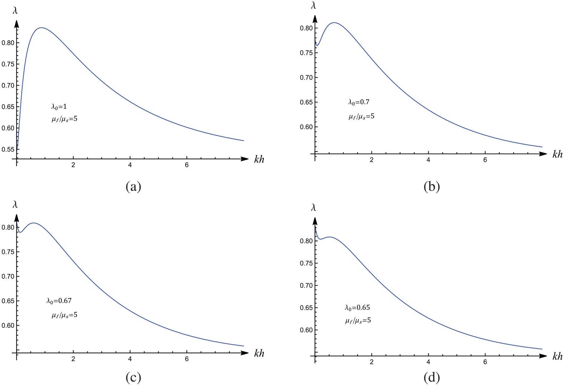
This study is concerned with the regime where $r$ is around $1/5$ which is relevant in biological applications [36]. It is found that in this regime there exists the possibility that with a prestretch ${\lambda }_0<1$ , the critical wavenumber becomes 0; see Figure 2(d). The rest of this article is divided into five sections as follows. After formulating the problem in the following section, we present the necessary linear analysis in Section 3 and show how bifurcation with zero wavenumber arises. In Section 4, we carry out a weakly nonlinear post-buckling analysis and discuss solutions of the resulting amplitude equations. This article is concluded in Section 5 with a summary and some further discussions.

2. Problem formulation

We first summarize the governing equations for a general homogeneous elastic body $B$ which is composed of a non-heat-conducting incompressible elastic material. The elastic body $B$ is assumed to possess an initial unstressed state $B_0$ . A static finite deformation brings $B_0$ to an equilibrium configuration denoted by $B_e$ . To study the stability properties of $B_e$ , we superimpose on $B_e$ a small amplitude perturbation, and the resulting configuration, termed the current configuration, is denoted by $B_t$ . The position vectors of a representative material particle relative to a common rectangular coordinate system are denoted by $\mathit{X}$ (with components $X_A$ ), $\mathit{x}$ (with components $x_i$ ) and $\tilde{\mathit{x}}$ (with components ${\tilde{x}}_i$ ) in $B_0,B_e$ and $B_t$ , respectively. We write

$$\tilde{\mathit{x}}(\mathit{X})=\mathit{x}(\mathit{X})+\mathit{u}(\mathit{x}),$$

(1)

where $\mathit{u}(\mathit{x})$ is the small-amplitude incremental displacement associated with the deformation $B_e\to B_t$ .

The deformation gradients arising from the deformations $B_0\to B_t$ and $B_0\to B_e$ are denoted by $\tilde{\mathit{F}}$ and $\overline{\mathit{F}}$ respectively, and are defined by $d\tilde{\mathit{x}}=\tilde{\mathit{F}}d\mathit{X}$ and $d\mathit{x}=\overline{\mathit{F}}d\mathit{X}$ . It then follows that

$${\tilde{F}}_{\mathrm{iA}}={\overline{F}}_{\mathrm{iA}}+u_{i,A}={\overline{F}}_{\mathrm{iA}}+u_{i,j}{\overline{F}}_{\mathrm{jA}},$$

(2)

where here and henceforth $u_{i,A}=\partial u_i/\partial X_A$ and $u_{i,j}=\partial u_i/\partial x_j$ .

We assume that the material is hyperelastic with a strain energy function given by

$$W=\frac{\mu }{2}(I_1-2-2\log (J))+\frac{\mu \nu }{1-2\nu }(J-1{)}^2,$$

(3)

where $J=\det \mathit{F}$ , $I_1=\mathrm{tr}({\mathit{F}}^T\mathit{F})$ with $\mathit{F}$ denoting the general deformation gradient. The $\mu$ and $\nu$ denote the ground state shear modulus and Poisson’s ratio, respectively. The neo-Hookean material model is recovered by taking the limit $\nu \to 0.5$ . We take $\nu =0.4999$ in all of our numerical examples, and so we will effectively be considering an incompressible hyperelastic material.

The general nominal stress tensor $(S_{\mathrm{Ai}})$ and its two specializations are computed according to

$$S_{\mathrm{Ai}}=\frac{\partial W}{\partial F_{\mathrm{iA}}},{\overline{S}}_{\mathrm{Ai}}={\frac{\partial W}{\partial F_{\mathrm{iA}}}|}_{\mathit{F}=\overline{\mathit{F}}},{\tilde{S}}_{\mathrm{Ai}}={\frac{\partial W}{\partial F_{\mathrm{iA}}}|}_{\mathit{F}=\tilde{\mathit{F}}}.$$

(4)

Define an incremental stress tensor $\chi$ through

$${\chi }_{\mathrm{ij}}={\overline{J}}^{-1}{\overline{F}}_{\mathrm{jA}}({\tilde{S}}_{\mathrm{Ai}}-{\overline{S}}_{\mathrm{Ai}}).$$

(5)

It then follows from the identify $({\overline{J}}^{-1}{\overline{F}}_{\mathrm{jA}}{)}_{,j}=0$ and the equilibrium equations ${\tilde{S}}_{\mathrm{Ai},A}=0$ and ${\overline{S}}_{\mathrm{Ai},A}=0$ that

$${\chi }_{\mathrm{ij},j}=0.$$

(6)

Expanding $\tilde{S}$ around $F=\overline{F}$ , we obtain

$${\chi }_{\mathrm{ij}}={\mathcal{A}}_{\mathrm{jilk}}^{(1)}{u}_{k,l}+\frac{1}{2}{\mathcal{A}}_{\mathrm{jilknm}}^{(2)}{u}_{k,l}{u}_{m,n}+\cdots ,$$

(7)

where ${\mathcal{A}}_{\mathrm{jilk}}^{(1)}$ and ${\mathcal{A}}_{\mathrm{jilknm}}^{(2)}$ are the first-order and second-order instantaneous elastic moduli defined by

$${\mathcal{A}}_{\mathrm{jilk}}^{(1)}={\overline{J}}^{-1}{\overline{F}}_{\mathrm{jA}}{\overline{F}}_{\mathrm{lB}}{\frac{{\partial }^{2}W}{\partial F_{\mathrm{iA}}\partial F_{\mathrm{kB}}}|}_{\mathbf{F}=\overline{\mathbf{F}}},{\mathcal{A}}_{\mathrm{jilknm}}^{(2)}={\overline{J}}^{-1}{\overline{F}}_{\mathrm{jA}}{\overline{F}}_{\mathrm{lB}}{\overline{F}}_{\mathrm{nC}}{\frac{{\partial }^{3}W}{\partial F_{\mathrm{iA}}\partial F_{\mathrm{kB}}\partial F_{\mathrm{mC}}}|}_{\mathbf{F}=\overline{\mathbf{F}}}.$$

(8)

Now consider an infinitesimal surface area $\mathrm{da}$ in $B_e$ with unit normal $\mathit{n}$ , and denote the image of $(\mathit{n},\mathrm{da})$ in $B_0$ by $(\mathit{N},\mathrm{dA})$ . With the use of Nanson’s formula $\mathit{n}\mathrm{da}=\overline{J}{\overline{F}}^{-T}\mathit{N}\mathrm{dA}$ , we have

$${\tilde{S}}^T\mathit{N}\mathrm{dA}={\overline{J}}^{-1}{\tilde{S}}^T{\overline{F}}^T\mathit{n}\mathrm{da}.$$

(9)

Thus, ${\overline{J}}^{-1}{\tilde{S}}^T{\overline{F}}^T\mathit{n}$ denotes the force per unit area on the surface $\mathit{n}\mathrm{da}$ and it must be continuous on any interface. It is also true when $\mathit{u}\equiv 0$ , that is if $\tilde{S}$ is replaced by $\overline{S}$ . Thus, ${\overline{J}}^{-1}({\tilde{S}}^T-{\overline{S}}^T){\overline{F}}^T\mathit{n}$ must be continuous on any interface. This, of course, is simply $\chi \mathit{n}$ . Note that the continuity of $\chi \mathit{n}$ across an interface is independent of how $\overline{F}$ on each side is produced. This fact is convenient for the current study where even the in-plane stretches on the two sides of the interface are allowed to be different.

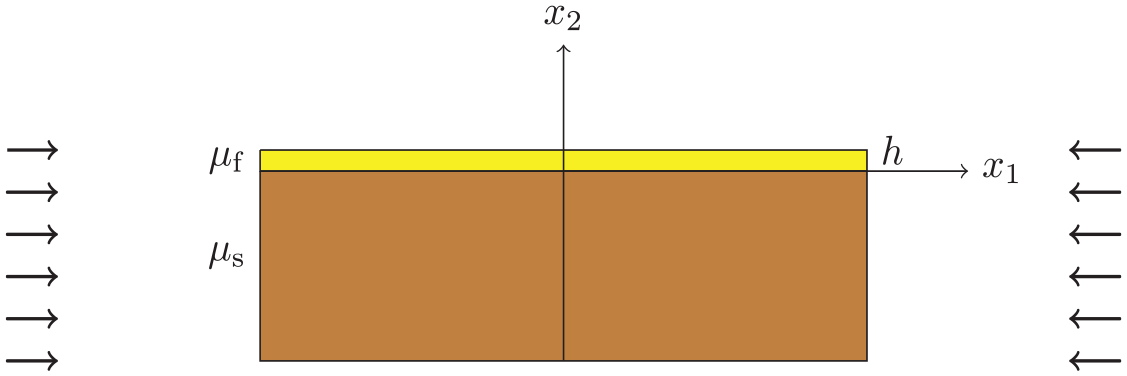
The above governing equations will now be applied to a film/substrate bilayer structure defined by $-\infty <x_2<h$ with $x_2=0$ corresponding to the interface and $h$ denoting the film thickness in $B_e$ ; see Figure 1. The substrate is assumed to have experienced a prestretch denoted by ${\lambda }_0$ in the $x_1-\mathrm{direction}$ before it is bonded to the film and subjected to a further stretch $\lambda$ together with the film. Thus, in the finitely deformed configuration $B_e$ , the stretches in the film and substrate are given by $\lambda$ and ${\lambda }_0\lambda$ , respectively. The relative stiffness of the film and substrate is characterized by the modulus ratio $r$ defined by

$$r={\mu }_{\mathrm{s}}/{\mu }_{\mathrm{f}},$$

(10)

where ${\mu }_{\mathrm{s}}$ and ${\mu }_{\mathrm{f}}$ denote the ground state shear moduli of the substrate and film, respectively.

Figure 1.

A film/substrate bilayer with the film and substrate occupying the regions $0<x_2<h$ and $-\infty <x_2<0$ , respectively. A uniaxial compression is applied to induce surface wrinkling.

3. Linear analysis

The linearized problem consists of solving the equilibrium equations

$${\tilde{\mathcal{A}}}_{\mathrm{jilk}}^{(1)}{\tilde{u}}_{k,\mathrm{lj}}=0,0<x_2<h,$$

(11)

$${\mathcal{A}}_{\mathrm{jilk}}^{(1)}{u}_{k,\mathrm{lj}}=0,-\infty <x_2<0,$$

(12)

subject to the traction-free boundary conditions

$${\tilde{\mathcal{A}}}_{2\mathrm{ilk}}^{(1)}{\tilde{u}}_{k,l}=0,x_2=h,$$

(13)

the continuity conditions

$${\tilde{\mathcal{A}}}_{2\mathrm{ilk}}^{(1)}{\tilde{u}}_{k,l}={\mathcal{A}}_{2\mathrm{ilk}}^{(1)}{u}_{k,l},{\tilde{u}}_i=u_i,x_2=0,$$

(14)

and the decay conditions

$$u_i\to 0,\mathrm{a}s{X}_2\to -\infty .$$

(15)

In the above expressions and hereafter, we use a superimposed tilde (e.g. ${\tilde{\mathcal{A}}}_{\mathrm{jilk}}^{(1)}$ ) to signify association with the film.

We look for a normal mode solution of the form

$$\{\tilde{\mathit{u}},\mathit{u}\}=\{\tilde{\mathit{v}}(x_2),\mathit{v}(x_2)\}{\mathrm{e}}^{\mathrm{i}k{x}_1}+\mathrm{c}.\mathrm{c},$$

(16)

where $k$ is the wavenumber, $\tilde{\mathit{v}}(x_2)$ and $\mathit{v}(x_2)$ are vector functions to be determined, and “c.c." denotes the complex conjugate of the preceding term. The reduced eigenvalue problem for $\tilde{\mathit{v}}(x_2)$ and $v(x_2)$ can easily be solved with the aid of Mathematica [37]. The resulting bifurcation condition is given by the determinant of a $6\times 6$ matrix equal to zero, and is of the form

$$f(\lambda ,{\lambda }_0,r,\mathrm{kh})=0,$$

(17)

where $f$ has an explicit expression but is not written out for the sake of brevity. A typical set of solutions of the above equation is presented in Figure 2(a)–(d) for different values of ${\lambda }_0$ with $r$ fixed at $1/5$ . We observe that $\mathrm{kh}=0$ corresponds to the absence of the film and so the corresponding stretch value is the critical value for the Biot problem, which is equal to $0.5437/{\lambda }_0$ in the current case, where $0.5437$ is the critical stretch when ${\lambda }_0=1$ . Thus, the bifurcation curves in the four plots cut the vertical axis at $\lambda =0.5437,0.7767,0.8115$ , and $0.8364$ , respectively. In the other extreme $\mathrm{kh}\to \infty$ , the film behaves like a half-space and so the associated limiting value of $\lambda$ is the critical value for the Biot problem associated with the film. Since the film and substrate have the same Poisson’s ratio, this value is again $0.5437$ , as can be seen in Figure 2(a). Note that there is another branch that cuts the $\mathrm{kh}-\mathrm{axis}$ at a finite value and tends to the critical stretch value for the interface mode in the limit $\mathrm{kh}\to \infty$ [5]. Since this branch is always below the branch shown, it is of no interest as far as determination of the stretch maximum is concerned.

Figure 2.

Evolution of the bifurcation curve with respect to the prestretch ${\lambda }_0$ in the substrate.

A novel feature can be seen in Figure 2 that does not seem to have been noted in previous investigations. As ${\lambda }_0$ is reduced gradually, the cut-off point of the bifurcation curve at $\mathrm{kh}=0$ keeps moving up (since $\lambda {|}_{\mathrm{kh}=0}=0.5437/{\lambda }_0$ ). This moving-up first creates an additional stretch minimum (see Figure 2(b)) and eventually the cut-off point becomes even higher than the local stretch maximum (see Figure 2(d)). There exists a threshold value of ${\lambda }_0$ at which the stretch value at $\mathrm{kh}=0$ is equal to its local maximum. The post-buckling behavior at this particular value of ${\lambda }_0$ is likely to be extremely interesting due to mode interaction, but the interest in the current study will be focused on the case when ${\lambda }_0$ is less than the above-mentioned threshold value so that the global stretch maximum occurs at $\mathrm{kh}=0$ . In other words, the critical mode has zero mode number, or equivalently infinite wavelength. Our interest in the next section will be in the characterization of the post-bifurcation solutions.

It is natural to ask if the mode-switching observed above occurs for all values of the modulus ratio. In view of the fact that creases will form on the surface of the substrate when ${\lambda }_0$ reaches $0.6422$ [38], we restrict ${\lambda }_0$ to the interval $(0.6422,1)$ . At the lower end ${\lambda }_0=0.6422$ , the bifurcation curve will cut the vertical axis at $\lambda =0.5437/0.6422=0.8466$ . Since the critical stretch in the limit $r\to 0$ behaves like $1-(1+{\lambda }_0^2{)}^{2/3}(3r/2{)}^{2/3}/4$ [29], it is clear that this stretch would be larger than $0.8466$ if $r$ were sufficiently small. As a crude estimation, equating this expression to 0.8466 yields $r=0.2269$ . A more precise calculation yields $r=0.1427$ or $r\approx 1/7$ . It can then be concluded that the stretch value at $\mathrm{kh}=0$ can be larger than the local maximum only if $r>1/7$ , that is ${\mu }_{\mathrm{f}}/{\mu }_{\mathrm{s}}<7$ .

4. Weakly nonlinear analysis

It was seen in the previous section that when ${\lambda }_0$ is decreased below a certain value that depends on the modulus ratio $r$ , the global maximum of $\lambda$ is attained at $\mathrm{kh}=0$ . It can be shown that around $\mathrm{kh}=0$ the behavior of $\lambda$ is linear, that is

$$\lambda ={\lambda }_{\mathrm{cr}}+d_1(\mathrm{kh})+O((\mathrm{kh}{)}^2),d_1<0,$$

(18)

where ${\lambda }_{\mathrm{cr}}=0.5437/{\lambda }_0$ when Poisson’s ratio is $0.4999$ , and the coefficient $d_1$ has an explicit expression that will be derived later. This means that if we take

$$\lambda ={\lambda }_{\mathrm{cr}}+\epsilon \hat{\lambda },$$

(19)

where $\epsilon$ is a small parameter characterizing the order of derivation of $\lambda$ from the critical value ${\lambda }_{\mathrm{cr}}$ , then $\mathrm{kh}$ will be of order $\epsilon$ . Without loss of generality, we may use $1/k$ as the lengthscale to non-dimensionalize all the length variables and parameters. As a result, we may take $k=1$ and write $h=\epsilon h_0$ with $h_0$ an $O(1)$ constant. We look for an asymptotic solution of the form

$$\mathit{u}=\{\begin{array}{cc}\epsilon {\mathit{u}}^{(1)}(x_1,x_2)+{\epsilon }^2{\mathit{u}}^{(2)}(x_1,x_2)+\cdots ,\hfill & -\infty <x_2<0,\hfill \\ \multicolumn{1}{c}{\epsilon {\tilde{\mathit{u}}}^{(1)}(x_1,Y)+{\epsilon }^2{\tilde{\mathit{u}}}^{(2)}(x_1,Y)+\cdots ,}& 0<Y<h_0,\hfill \end{array}$$

(20)

where a stretched variable $Y=x_2/\epsilon$ has been introduced for the film.

It can be shown that ${\tilde{\mathit{u}}}^{(1)}$ is independent of $Y$ , nonlinear terms do not come into play in the leading analysis for the film, and the following relationship can be derived (see, e.g., [39]):

$$({\tilde{\chi }}_{i2}){|}_{Y=0}={\epsilon }^2{h}_0(\tilde{Q}-\tilde{R}{\tilde{T}}^{-1}{\tilde{R}}^T){\tilde{\mathit{u}}}_{,11}^{(1)}+O({\epsilon }^3),$$

(21)

where $\tilde{T}$ , $\tilde{R}$ and $\tilde{Q}$ are $2\times 2$ matrices with components

$${\tilde{T}}_{\mathrm{ik}}={{\tilde{\mathcal{A}}}_{2i2k}^{(1)}|}_{\lambda ={\lambda }_{\mathrm{cr}}},{\tilde{R}}_{\mathrm{ik}}={{\tilde{\mathcal{A}}}_{1i2k}^{(1)}|}_{\lambda ={\lambda }_{\mathrm{cr}}},{\tilde{Q}}_{\mathrm{ik}}={{\tilde{\mathcal{A}}}_{1i1k}^{(1)}|}_{\lambda ={\lambda }_{\mathrm{cr}}}.$$

(22)

Because of continuity of displacement and traction across the interface, the ${\tilde{\mathit{u}}}^{(1)}$ and $({\tilde{\chi }}_{2i})$ in equation (21) are equal to their counterparts in the half-space. Equation (21) then becomes an effective boundary condition to be imposed on the surface of the half-space.

We now proceed to solve the problem associated with the substrate. On substituting equation (20) into the equilibrium equations and boundary conditions for the substrate, we obtain

$${\mathcal{A}}_{\mathrm{jilk}}^{(1)}{u}_{k,\mathrm{lj}}^{(1)}=0,-\infty <x_2<0,$$

(23)

$${\mathcal{A}}_{2\mathrm{ilk}}^{(1)}{u}_{k,l}^{(1)}=0,x_2=0,$$

(24)

to leading order, and

$${\mathcal{A}}_{\mathrm{jilk}}^{(1)}{u}_{k,\mathrm{lj}}^{(2)}=-\hat{\lambda }{\mathcal{A}\prime }_{\mathrm{jilk}}^{(1)}{u}_{k,\mathrm{lj}}^{(1)}-{\mathcal{A}}_{\mathrm{jilknm}}^{(2)}{u}_{k,\mathrm{lj}}^{(1)}{u}_{m,n}^{(1)},-\infty <x_2<0$$

(25)

$${\mathcal{A}}_{2\mathrm{ilk}}^{(1)}{u}_{k,l}^{(2)}=-\hat{\lambda }{\mathcal{A}\prime }_{2\mathrm{ilk}}^{(1)}{u}_{k,l}^{(1)}-\frac{1}{2}{\mathcal{A}}_{2\mathrm{ilknm}}^{(2)}{u}_{k,l}^{(1)}{u}_{m,n}^{(1)}+r_i,x_2=0,$$

(26)

at order ${\epsilon }^2$ , where $r_i$ is the $i\mathrm{th}$ component of the vector defined by

$$\mathit{r}=h_0(\tilde{Q}-\tilde{R}{\tilde{T}}^{-1}{\tilde{R}}^T){\mathit{u}}_{,11}^{(1)},$$

(27)

${\mathcal{A}\prime }_{\mathrm{jilk}}^{(1)}=d{\mathcal{A}}_{\mathrm{jilk}}^{(1)}/d\lambda$ , and all the moduli are evaluated at $\lambda ={\lambda }_{\mathrm{cr}}$ .

The leading order problem (23) and (24) is the classical Biot problem [40]. There exist non-trivial solutions of the form

$$\mathit{u}=\mathit{z}(\mathrm{i}k{x}_2){\mathrm{e}}^{\mathrm{i}k{x}_1},\mathit{z}(\mathrm{i}k{x}_2)={\mathrm{e}}^{k{x}_{2}E}\mathit{d},k>0,$$

(28)

provided the leading order stretch ${\lambda }_{\mathrm{cr}}$ and the constant vector $\mathit{d}$ satisfy the conditions

$$\det M=0,M\mathit{d}=0.$$

(29)

In the above expressions, $M$ is the positive semi-definite surface-impedance matrix satisfying the matrix Riccati equation

$$(M+\mathrm{i}R)T^{-1}(M-\mathrm{i}{R}^T)-Q=0,$$

(30)

and the matrix $E$ is related to $M$ by

$$E=T^{-1}(M-\mathrm{i}{R}^T),$$

(31)

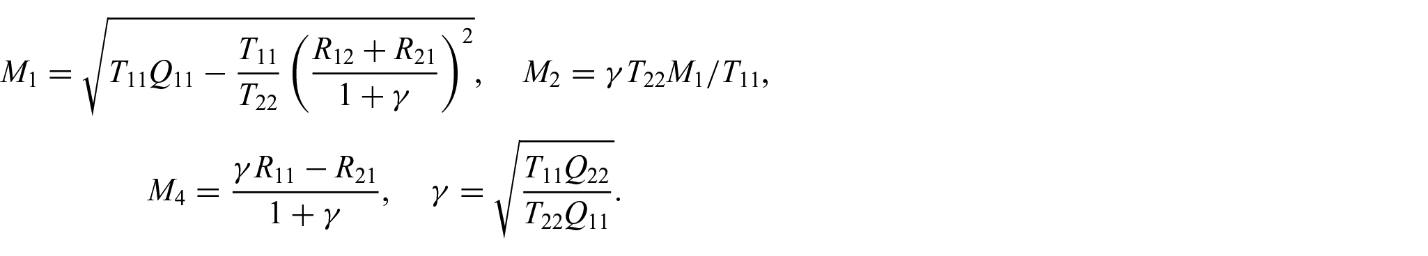
where $T$ , $R$ , and $Q$ are $2\times 2$ matrices with components

$$T_{\mathrm{ik}}={{\mathcal{A}}_{2i2k}^{(1)}|}_{\lambda ={\lambda }_{\mathrm{cr}}},R_{\mathrm{ik}}={{\mathcal{A}}_{1i2k}^{(1)}|}_{\lambda ={\lambda }_{\mathrm{cr}}},Q_{\mathrm{ik}}={{\mathcal{A}}_{1i1k}^{(1)}|}_{\lambda ={\lambda }_{\mathrm{cr}}}.$$

(32)

See, for instance, Biryukov [41], Barnett and Lothe [42] or Fu and Mielke [43]. In the current case where the principal axes of the pre-stress coincide with the coordinate axes, the $M$ has the explicit expression

$$M=\left(\begin{array}{cc}{M}_1\hfill & -\mathrm{i}{M}_4\hfill \\ \multicolumn{1}{c}{\mathrm{i}{M}_4}& M_2\hfill \end{array}\right),$$

(33)

with

$$\begin{array}{c}{M}_1=\sqrt{T_{11}{Q}_{11}-\frac{T_{11}}{T_{22}}{\left(\frac{R_{12}+R_{21}}{1+\gamma }\right)}^2},M_2=\gamma T_{22}{M}_1/T_{11},\hfill \\ \multicolumn{1}{c}{M_4=\frac{\gamma R_{11}-R_{21}}{1+\gamma },\gamma =\sqrt{\frac{T_{11}{Q}_{22}}{T_{22}{Q}_{11}}}.}\end{array}$$

With the use of these expressions, the unique solution of equation (29)₁ is found to be ${\lambda }_{\mathrm{cr}}=0.5437/{\lambda }_0$ when $\nu =0.4999$ , as anticipated earlier.

For the leading-order problem, a general solution is given by the Fourier expansion

$${\mathit{u}}^{(1)}=\sum _{q=-\infty }^{\infty }{A}_q\mathit{z}(\mathrm{i}q{x}_2){\mathrm{e}}^{\mathrm{i}q{x}_1},(q\ne 0),$$

(34)

where $A_q(q=\pm 1,\pm 2,\dots )$ are constants to be determined and $\mathit{z}(\mathrm{i}q{x}_2)$ for $q>0$ is defined by equation (28)₂. We impose the conditions

$$\mathit{z}(\mathrm{i}q{x}_2)=\overline{\mathit{z}(-\mathrm{i}q{x}_2)},A_q=\overline{A_{-q}},q<0,$$

(35)

to satisfy the decay condition and to ensure the reality of ${\mathit{u}}^{(1)}$ in equation (34), where an overbar signifies complex conjugation. Note that equation (34) could be replaced by a Fourier transform, but the Fourier series representation is more convenient for numerical computations. It is known that the Fourier expansion is also capable of capturing localized solutions [44]. Note also that the fundamental wavenumber in equation (34) is taken to be one; this is because we have used the inverse of the actual wavenumber as the length unit.

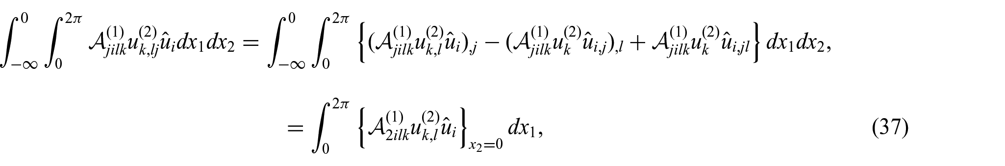
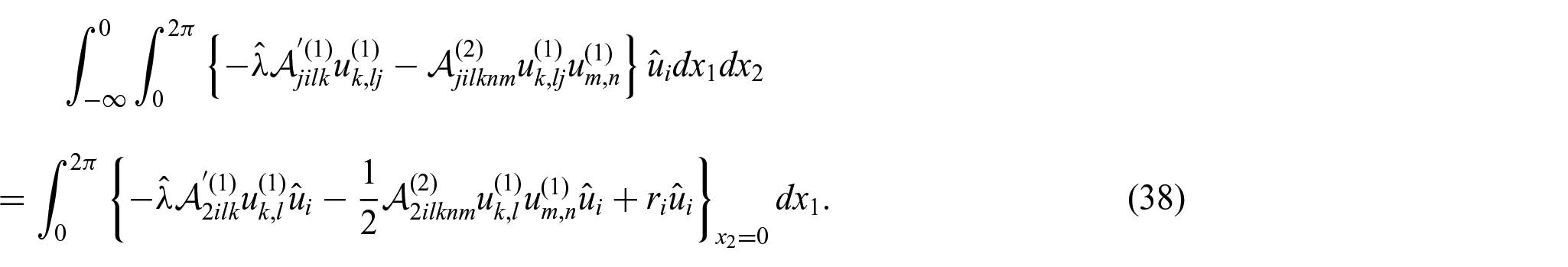
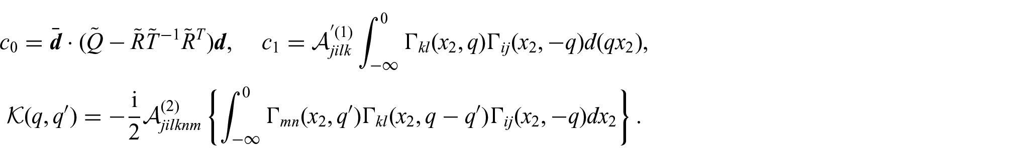
To derive the amplitude equations satisfied by $A_q(q=1,2,...)$ , we define a virtual displacement field by

$$\hat{\mathit{u}}=\overline{\mathit{z}(\mathrm{i}q{x}_2)}{\mathrm{e}}^{-\mathrm{i}q{x}_1}.$$

(36)

It then follows with the use of the divergence theorem and the property ${\mathcal{A}}_{\mathrm{jilk}}^{(1)}={\mathcal{A}}_{\mathrm{lkji}}^{(1)}$ that

$$\begin{array}{c}{\int }_{-\infty }^0{\int }_0^{2\pi }{\mathcal{A}}_{\mathrm{jilk}}^{(1)}{u}_{k,\mathrm{lj}}^{(2)}{\hat{u}}_{i}d{x}_{1}d{x}_2={\int }_{-\infty }^0{\int }_0^{2\pi }\{{({\mathcal{A}}_{\mathrm{jilk}}^{(1)}{u}_{k,l}^{(2)}{\hat{u}}_i)}_{,j}-{({\mathcal{A}}_{\mathrm{jilk}}^{(1)}{u}_k^{(2)}{\hat{u}}_{i,j})}_{,l}+{\mathcal{A}}_{\mathrm{jilk}}^{(1)}{u}_k^{(2)}{\hat{u}}_{i,\mathrm{jl}}\}d{x}_{1}d{x}_2,\hfill \\ \multicolumn{1}{c}{={\int }_0^{2\pi }{\left\{{\mathcal{A}}_{2\mathrm{ilk}}^{(1)}{u}_{k,l}^{(2)}{\hat{u}}_i\right\}}_{x_2=0}d{x}_1,}\end{array}$$

(37)

where use has also been made of the facts that (i) $\hat{\mathit{u}}$ satisfies the leading order problem (23) and (24), (ii) both ${\mathit{u}}^{(2)}$ and $\hat{\mathit{u}}$ are $2\pi -\mathrm{periodic}$ so that the integrals on $x_1=0$ and $x_1=2\pi$ cancel each other, and (iii) both ${\mathit{u}}^{(2)}$ and $\hat{\mathit{u}}$ decay to zero as $x_2\to -\infty$ .

On using equations (25) and (26) to eliminate the unknown field ${\mathit{u}}^{(2)}$ in the above expression, we arrive at

$$\begin{array}{c}{\int }_{-\infty }^0{\int }_0^{2\pi }\{-\hat{\lambda }{\mathcal{A}\prime }_{\mathrm{jilk}}^{(1)}{u}_{k,\mathrm{lj}}^{(1)}-{\mathcal{A}}_{\mathrm{jilknm}}^{(2)}{u}_{k,\mathrm{lj}}^{(1)}{u}_{m,n}^{(1)}\}{\hat{u}}_{i}d{x}_{1}d{x}_2\hfill \\ \multicolumn{1}{c}{={\int }_0^{2\pi }{\{-\hat{\lambda }{\mathcal{A}\prime }_{2\mathrm{ilk}}^{(1)}{u}_{k,l}^{(1)}{\hat{u}}_i-\frac{1}{2}{\mathcal{A}}_{2\mathrm{ilknm}}^{(2)}{u}_{k,l}^{(1)}{u}_{m,n}^{(1)}{\hat{u}}_i+r_i{\hat{u}}_i\}}_{x_2=0}d{x}_1.}\end{array}$$

(38)

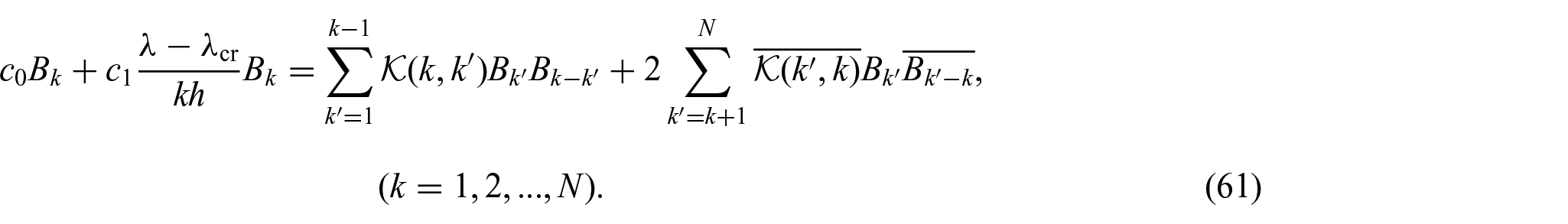
With the further use of the divergence theorem, the above equation can be reduced to

$${\int }_{-\infty }^0{\int }_0^{2\pi }\{\hat{\lambda }{\mathcal{A}\prime }_{\mathrm{jilk}}^{(1)}{u}_{k,l}^{(1)}+\frac{1}{2}{\mathcal{A}}_{\mathrm{jilknm}}^{(2)}{u}_{k,l}^{(1)}{u}_{m,n}^{(1)}\}{\hat{u}}_{i,j}d{x}_{1}d{x}_2={\int }_0^{2\pi }{{\hat{u}}_i{r}_i|}_{x_2=0}d{x}_1.$$

(39)

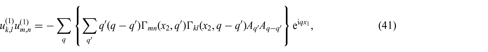
To evaluate the integrals in the above equation, we first compute

$$u_{k,l}^{(1)}=\sum _q\mathrm{i}q{A}_q{\mathrm{\Gamma }}_{\mathrm{kl}}(x_2,q){\mathrm{e}}^{\mathrm{i}q{x}_1},u_{m,n}^{(1)}=\sum _{q^{\prime }}\mathrm{i}{q}^{\prime }{A}_{q^{\prime }}{\mathrm{\Gamma }}_{\mathrm{mn}}(x_2,q^{\prime }){\mathrm{e}}^{\mathrm{i}{q}^{\prime }{x}_1},$$

(40)

$$u_{k,l}^{(1)}{u}_{m,n}^{(1)}=-\sum _q\{\sum _{q^{\prime }}{q}^{\prime }(q-q^{\prime }){\mathrm{\Gamma }}_{\mathrm{mn}}(x_2,q^{\prime }){\mathrm{\Gamma }}_{\mathrm{kl}}(x_2,q-q^{\prime })A_{q^{\prime }}{A}_{q-q^{\prime }}\}{\mathrm{e}}^{\mathrm{i}q{x}_1},$$

(41)

where

$${\mathrm{\Gamma }}_{\mathrm{kl}}(x_2,q)={\delta }_{1l}{z}_k(\mathrm{i}q{x}_2)+{\delta }_{2l}{z}_k^{\prime }(\mathrm{i}q{x}_2).$$

(42)

The ${\mathrm{\Gamma }}_{\mathrm{kl}}$ defined above inherits from equation (35) the property

$${\mathrm{\Gamma }}_{\mathrm{kl}}(x_2,-q)=\overline{{\mathrm{\Gamma }}_{\mathrm{kl}}(x_2,q)},q\ne 0.$$

(43)

We also have

$${\hat{u}}_{i,j}=-\mathrm{i}q{\mathrm{\Gamma }}_{\mathrm{ij}}(x_2,-q){\mathrm{e}}^{-\mathrm{i}q{x}_1}.$$

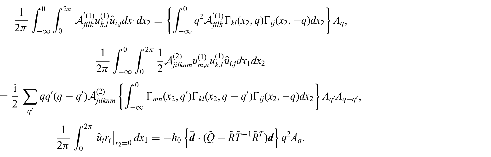
It then follows that

$$\begin{array}{c}\frac{1}{2\pi }{\int }_{-\infty }^0{\int }_0^{2\pi }{\mathcal{A}\prime }_{\mathrm{jilk}}^{(1)}{u}_{k,l}^{(1)}{\hat{u}}_{i,j}d{x}_{1}d{x}_2=\{{\int }_{-\infty }^0{q}^2{\mathcal{A}\prime }_{\mathrm{jilk}}^{(1)}{\mathrm{\Gamma }}_{\mathrm{kl}}(x_2,q){\mathrm{\Gamma }}_{\mathrm{ij}}(x_2,-q)d{x}_2\}{A}_q,\hfill \\ \multicolumn{1}{c}{\frac{1}{2\pi }{\int }_{-\infty }^0{\int }_0^{2\pi }\frac{1}{2}{\mathcal{A}}_{\mathrm{jilknm}}^{(2)}{u}_{m,n}^{(1)}{u}_{k,l}^{(1)}{\hat{u}}_{i,j}d{x}_{1}d{x}_2}\\ \multicolumn{1}{c}{=\frac{\mathrm{i}}{2}\sum _{q^{\prime }}{\mathrm{qq}}^{\prime }(q-q^{\prime }){\mathcal{A}}_{\mathrm{jilknm}}^{(2)}\{{\int }_{-\infty }^0{\mathrm{\Gamma }}_{\mathrm{mn}}(x_2,q^{\prime }){\mathrm{\Gamma }}_{\mathrm{kl}}(x_2,q-q^{\prime }){\mathrm{\Gamma }}_{\mathrm{ij}}(x_2,-q)d{x}_2\}{A}_{q^{\prime }}{A}_{q-q^{\prime }},}\\ \multicolumn{1}{c}{\frac{1}{2\pi }{\int }_0^{2\pi }{{\hat{u}}_i{r}_i|}_{x_2=0}d{x}_1=-h_0\{\overline{\mathit{d}}·(\tilde{Q}-\tilde{R}{\tilde{T}}^{-1}{\tilde{R}}^T)\mathit{d}\}{q}^2{A}_q.}\end{array}$$

Substituting these expressions into equation (39) then gives

$$\begin{array}{c}\hat{\lambda }\{{\int }_{-\infty }^0{\mathcal{A}\prime }_{\mathrm{jilk}}^{(1)}{\mathrm{\Gamma }}_{\mathrm{kl}}(x_2,q){\mathrm{\Gamma }}_{\mathrm{ij}}(x_2,-q)d(q{x}_2)\}{A}_q+h_0\{\overline{\mathit{d}}·(\tilde{Q}-\tilde{R}{\tilde{T}}^{-1}{\tilde{R}}^T)\mathit{d}\}(q{A}_q)\hfill \\ \multicolumn{1}{c}{=-\frac{\mathrm{i}}{2}\sum _{q^{\prime }}{q}^{\prime }(q-q^{\prime }){\mathcal{A}}_{\mathrm{jilknm}}^{(2)}\{{\int }_{-\infty }^0{\mathrm{\Gamma }}_{\mathrm{mn}}(x_2,q^{\prime }){\mathrm{\Gamma }}_{\mathrm{kl}}(x_2,q-q^{\prime }){\mathrm{\Gamma }}_{\mathrm{ij}}(x_2,-q)d{x}_2\}{A}_{q^{\prime }}{A}_{q-q^{\prime }},}\end{array}$$

(44)

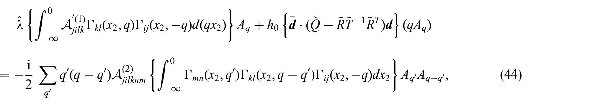
or equivalently,

$$c_0{h}_{0}q{A}_q+c_1\hat{\lambda }{A}_q=\sum _{q^{\prime }}{q}^{\prime }(q-q^{\prime })\mathcal{K}(q,q^{\prime })A_{q^{\prime }}{A}_{q-q^{\prime }},$$

(45)

where

$$\begin{array}{c}{c}_0=\overline{\mathit{d}}·(\tilde{Q}-\tilde{R}{\tilde{T}}^{-1}{\tilde{R}}^T)\mathit{d},c_1={\mathcal{A}\prime }_{\mathrm{jilk}}^{(1)}{\int }_{-\infty }^0{\mathrm{\Gamma }}_{\mathrm{kl}}(x_2,q){\mathrm{\Gamma }}_{\mathrm{ij}}(x_2,-q)d(q{x}_2),\hfill \\ \mathcal{K}(q,q^{\prime })=-\frac{\mathrm{i}}{2}{\mathcal{A}}_{\mathrm{jilknm}}^{(2)}\{{\int }_{-\infty }^0{\mathrm{\Gamma }}_{\mathrm{mn}}(x_2,q^{\prime }){\mathrm{\Gamma }}_{\mathrm{kl}}(x_2,q-q^{\prime }){\mathrm{\Gamma }}_{\mathrm{ij}}(x_2,-q)d{x}_2\}.\hfill \end{array}$$

It follows from the pairwise symmetry property of ${\mathcal{A}}_{\mathrm{jilknm}}^{(2)}$ (e.g. ${\mathcal{A}}_{\mathrm{jilknm}}^{(2)}={\mathcal{A}}_{\mathrm{jinmlk}}^{(2)}$ ) that

$$\mathcal{K}(q,q^{\prime })=\mathcal{K}(q,q-q^{\prime }),\mathcal{K}(q^{\prime },q)=-\overline{\mathcal{K}(q,q^{\prime })},q^{\prime }\ne q.$$

(46)

These identities hold irrespective of the signs of $q$ and $q^{\prime }$ . The form of equation (45) suggests the introduction of new amplitudes $B_q^{*}(q=1,2,...)$ through

$$B_q^{*}=q{A}_q,$$

(47)

which inherits from equation (35)₂, the property

$$B_{-q}^{*}=-\overline{B_q^{*}}.$$

(48)

Equation (45) then reduces to

$$c_0{h}_0{B}_q^{*}+\frac{1}{q}{c}_1\hat{\lambda }{B}_q^{*}=\sum _{q^{\prime }}\mathcal{K}(q,q^{\prime })B_{q^{\prime }}^{*}{B}_{q-q^{\prime }}^{*}.$$

(49)

To evaluate the integrals in $c_1$ and $\mathcal{K}(q,q^{\prime })$ explicitly, we rewrite the $\mathit{z}$ in the leading order solution (34) in the form

$$\mathit{z}(\mathrm{i}q{x}_2)=\sum _{\alpha =1}^2{c}_{\alpha }{\mathit{a}}^{(\alpha )}{\mathrm{e}}^{\mathrm{i}{p}_{\alpha }q{x}_2},q>0,$$

(50)

where $(p_{\alpha },{\mathit{a}}^{(\alpha )})$ $(\alpha =1,2)$ are the two solutions of the eigenvalue problem

$$(p^{2}T+p(R+R^T)+Q)\mathbf{a}=0$$

(51)

that satisfy the condition $\mathrm{Im}p<0$ , and $c_1$ and $c_2$ are the components of $\mathit{c}=[{\mathit{a}}^{(1)},{\mathit{a}}^{(2)}{]}^{-1}\mathit{d}$ .

To simplify notation, we use a modified summation convention whereby a Greek suffix repeated three times or more in a single term also implies summation over $\{1,2\}$ . Thus, equation (50) may be written simply as

$$\mathit{z}(\mathrm{i}q{x}_2)=c_{\alpha }{\mathit{a}}^{(\alpha )}{\mathrm{e}}^{\mathrm{i}{p}_{\alpha }q{x}_2}=c_{\beta }{\mathit{a}}^{(\beta )}{\mathrm{e}}^{\mathrm{i}{p}_{\beta }q{x}_2},q>0.$$

(52)

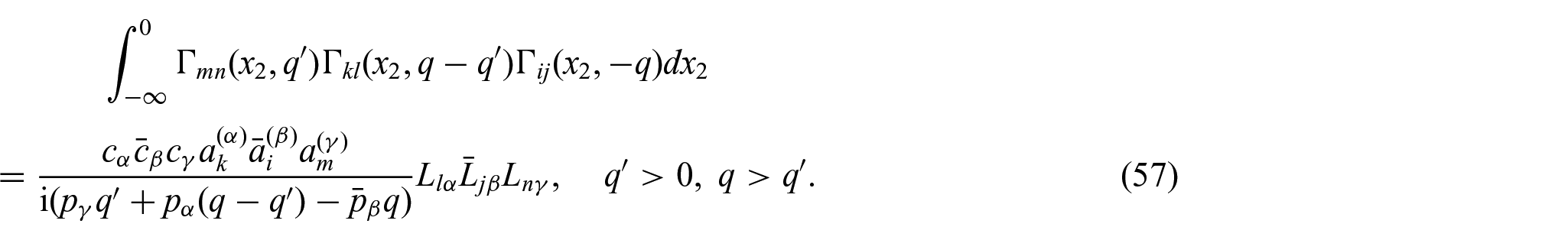
As a result, with the use of the notation $L_{l\alpha }={\delta }_{1l}+{\delta }_{2l}{p}_{\alpha }$ , we have

$${\mathrm{\Gamma }}_{\mathrm{kl}}(x_2,q)=L_{l\alpha }{c}_{\alpha }{a}_k^{(\alpha )}{\mathrm{e}}^{\mathrm{i}{p}_{\alpha }q{x}_2},q>0,$$

(53)

$${\mathrm{\Gamma }}_{\mathrm{mn}}(x_2,q^{\prime })=L_{n\gamma }{c}_{\gamma }{a}_m^{(\gamma )}{\mathrm{e}}^{\mathrm{i}{p}_{\gamma }{q}^{\prime }{x}_2},q^{\prime }>0,$$

(54)

$${\mathrm{\Gamma }}_{\mathrm{ij}}(x_2,-q)=\overline{{\mathrm{\Gamma }}_{\mathrm{ij}}(x_2,q)}={\overline{L}}_{j\beta }{\overline{c}}_{\beta }{\overline{a}}_i^{(\beta )}{\mathrm{e}}^{-\mathrm{i}{\overline{p}}_{\beta }q{x}_2},q>0.$$

(55)

It then follows that

$$\begin{array}{c}{\int }_{-\infty }^0{\mathrm{\Gamma }}_{\mathrm{kl}}(x_2,q){\mathrm{\Gamma }}_{\mathrm{ij}}(x_2,-q)d(q{x}_2)=\frac{c_{\alpha }{\overline{c}}_{\beta }{a}_k^{(\alpha )}{\overline{a}}_i^{(\beta )}}{\mathrm{i}(p_{\alpha }-{\overline{p}}_{\beta })}{L}_{l\alpha }{\overline{L}}_{j\beta },q>0,\hfill \end{array}$$

(56)

$$\begin{array}{c}\multicolumn{1}{c}{{\int }_{-\infty }^0{\mathrm{\Gamma }}_{\mathrm{mn}}(x_2,q^{\prime }){\mathrm{\Gamma }}_{\mathrm{kl}}(x_2,q-q^{\prime }){\mathrm{\Gamma }}_{\mathrm{ij}}(x_2,-q)d{x}_2}\\ \multicolumn{1}{c}{=\frac{c_{\alpha }{\overline{c}}_{\beta }{c}_{\gamma }{a}_k^{(\alpha )}{\overline{a}}_i^{(\beta )}{a}_m^{(\gamma )}}{\mathrm{i}(p_{\gamma }{q}^{\prime }+p_{\alpha }(q-q^{\prime })-{\overline{p}}_{\beta }q)}{L}_{l\alpha }{\overline{L}}_{j\beta }{L}_{n\gamma },q^{\prime }>0,q>q^{\prime }.}\end{array}$$

(57)

Thus, we have

$$c_1=\frac{c_{\alpha }{\overline{c}}_{\beta }{a}_k^{(\alpha )}{\overline{a}}_i^{(\beta )}}{\mathrm{i}(p_{\alpha }-{\overline{p}}_{\beta })}{\mathcal{A}\prime }_{\mathrm{jilk}}^{(1)}{L}_{l\alpha }{\overline{L}}_{j\beta },$$

(58)

$$\mathcal{K}(q,q^{\prime })=-\frac{1}{2}·\frac{c_{\alpha }{\overline{c}}_{\beta }{c}_{\gamma }{a}_k^{(\alpha )}{\overline{a}}_i^{(\beta )}{a}_m^{(\gamma )}}{p_{\gamma }{q}^{\prime }+p_{\alpha }(q-q^{\prime })-{\overline{p}}_{\beta }q}·{\mathcal{A}}_{\mathrm{jilknm}}^{(2)}{L}_{l\alpha }{\overline{L}}_{j\beta }{L}_{n\gamma },q^{\prime }>0,q>q^{\prime }.$$

(59)

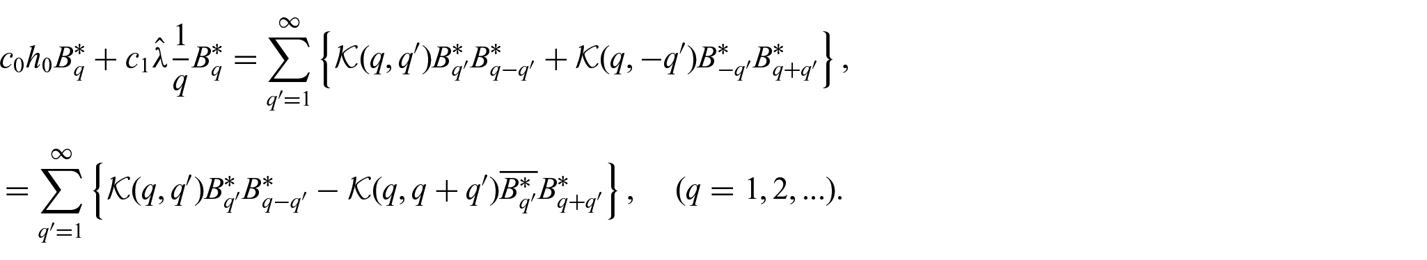
When $q$ and $q^{\prime }$ do not satisfy $q>q^{\prime }$ , the value of $\mathcal{K}(q,q^{\prime })$ is calculated with the aid of equation (46). As a result, the amplitude equation (49) for $q>0$ may be rewritten in the form

$$\begin{array}{c}{c}_0{h}_0{B}_q^{*}+c_1\hat{\lambda }\frac{1}{q}{B}_q^{*}=\sum _{q^{\prime }=1}^{\infty }\{\mathcal{K}(q,q^{\prime })B_{q^{\prime }}^{*}{B}_{q-q^{\prime }}^{*}+\mathcal{K}(q,-q^{\prime })B_{-q^{\prime }}^{*}{B}_{q+q^{\prime }}^{*}\},\hfill \\ =\sum _{q^{\prime }=1}^{\infty }\{\mathcal{K}(q,q^{\prime })B_{q^{\prime }}^{*}{B}_{q-q^{\prime }}^{*}-\mathcal{K}(q,q+q^{\prime })\overline{B_{q^{\prime }}^{*}}{B}_{q+q^{\prime }}^{*}\},(q=1,2,...).\hfill \end{array}$$

We now truncate the above infinite system by assuming that $B_{N+1}^{*}=B_{N+2}^{*}=\cdots =0$ with $N$ an integer. It then follows that

$$\begin{array}{c}{c}_0{h}_0{B}_q^{*}+c_1\hat{\lambda }\frac{1}{q}{B}_q^{*}=\sum _{q^{\prime }=1}^{q-1}\mathcal{K}(q,q^{\prime })B_{q^{\prime }}^{*}{B}_{q-q^{\prime }}^{*}-\sum _{q^{\prime }=q+1}^N\overline{\mathcal{K}(q^{\prime },q)}{B}_{q^{\prime }}^{*}{B}_{q-q^{\prime }}^{*}-\sum _{q^{\prime }=1}^{N-q}\mathcal{K}(q,q+q^{\prime })\overline{B_{q^{\prime }}^{*}}{B}_{q+q^{\prime }}^{*}\hfill \\ \multicolumn{1}{c}{=\sum _{q^{\prime }=1}^{q-1}\mathcal{K}(q,q^{\prime })B_{q^{\prime }}^{*}{B}_{q-q^{\prime }}^{*}+\sum _{q^{\prime }=q+1}^N\overline{\mathcal{K}(q^{\prime },q)}{B}_{q^{\prime }}^{*}\overline{B_{q^{\prime }-q}^{*}}-\sum _{m=q+1}^N\mathcal{K}(q,m)\overline{B_{m-q}^{*}}{B}_m^{*}}\\ \multicolumn{1}{c}{=\sum _{q^{\prime }=1}^{q-1}\mathcal{K}(q,q^{\prime })B_{q^{\prime }}^{*}{B}_{q-q^{\prime }}^{*}+2\sum _{q^{\prime }=q+1}^N\overline{\mathcal{K}(q^{\prime },q)}{B}_{q^{\prime }}^{*}\overline{B_{q^{\prime }-q}^{*}}.}\end{array}$$

(60)

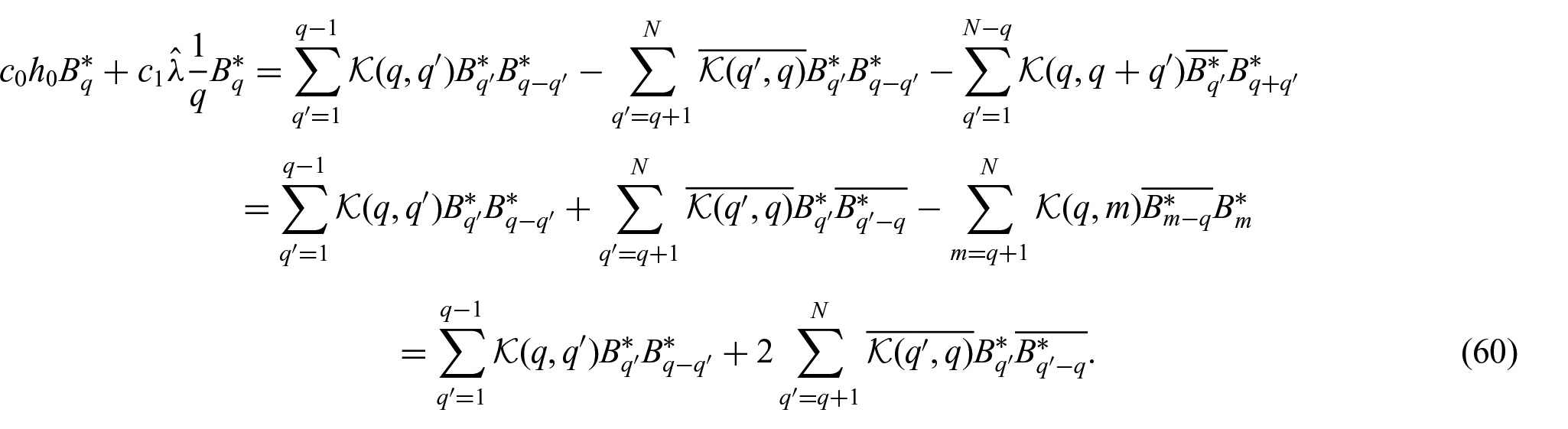
Multiplying the last equation by ${\epsilon }^2$ and writing $\epsilon B_q^{*}=h{B}_q$ , we obtain

$$\begin{array}{c}{c}_0{B}_k+c_1\frac{\lambda -{\lambda }_{\mathrm{cr}}}{\mathrm{kh}}{B}_k=\sum _{k^{\prime }=1}^{k-1}\mathcal{K}(k,k^{\prime })B_{k^{\prime }}{B}_{k-k^{\prime }}+2\sum _{k^{\prime }=k+1}^N\overline{\mathcal{K}(k^{\prime },k)}{B}_{k^{\prime }}\overline{B_{k^{\prime }-k}},\hfill \\ \multicolumn{1}{c}{(k=1,2,...,N).}\end{array}$$

(61)

It is seen that with the inverse of the actual fundamental wavenumber taken to be the length unit, the (relative) film thickness $h$ and stretch deviation $\lambda -{\lambda }_{\mathrm{cr}}$ appear in the above amplitude equations through the combination $(\lambda -{\lambda }_{\mathrm{cr}})/h$ . This means that the solutions are not changed if any change in $h$ is accompanied by the same change in $\lambda -{\lambda }_{\mathrm{cr}}$ . Thus, without loss of generality, we may fix $h$ and vary $\lambda -{\lambda }_{\mathrm{cr}}$ only. Also, we may ignore solutions in which $B_k$ are zero except when $k=\mathrm{Km}(m=1,2,...)$ with $K$ an integer. This is because this is the same solution when $h$ is replaced by $h/K$ , or equivalently if $h$ is fixed and $\lambda -{\lambda }_{\mathrm{cr}}$ is replaced by $(\lambda -{\lambda }_{\mathrm{cr}})/K$ .

Once a non-trivial solution is found, the associated surface elevation $u_2(x_1,0)$ and surface gradient $u_{2,1}(x_1,0)$ may, to leading order, be computed from

$$u_2(x_1,0)=2h(c_1{a}_2^{(1)}+c_2{a}_2^{(2)})\sum _{k=1}^N(B_k/k)\cos (k{x}_1),$$

(62)

$$u_{2,1}(x_1,0)=-2h(c_1{a}_2^{(1)}+c_2{a}_2^{(2)})\sum _{k=1}^N{B}_k\sin (k{x}_1).$$

(63)

For the current problem, $c_0,c_1$ and $\mathcal{K}(k,k^{\prime })$ are all real. Thus, we may look for a solution in which $B_k$ are all real.

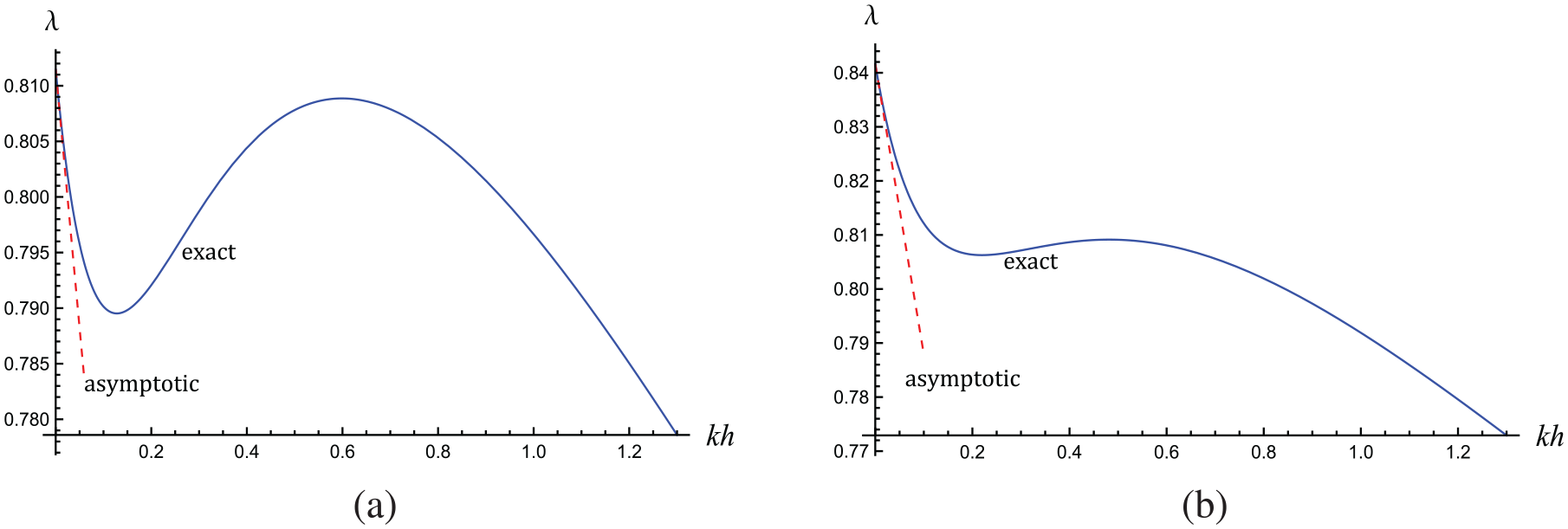
As a consistency check, we may neglect the nonlinear terms in equation (61) to obtain

$$\lambda -{\lambda }_{\mathrm{cr}}=-\frac{c_0}{c_1}(\mathrm{kh}).$$

(64)

An analytical expression for the coefficient $-c_0/c_1$ can be obtained, but is not written out here for brevity. Figure 3 shows the linear behavior given by equation (64) near $\mathrm{kh}=0$ together with the exact solution for two typical values of ${\lambda }_0$ .

Figure 3.

Comparison of asymptotic result (64) with the exact solution when (a) ${\lambda }_0=0.670$ and (b) ${\lambda }_0=0.646$ .

5. Numerical solutions

We now proceed to solve the system of amplitude equations (61) numerically. We start with the truncation number $N=2$ to obtain

$$B_1^2=\frac{(c_0+c_1{\lambda }_s)(2c_0+c_1{\lambda }_s)}{4{\mathcal{K}}_{21}^2},B_2=\frac{c_0+c_1{\lambda }_s}{2{\mathcal{K}}_{21}},$$

(65)

where

$${\lambda }_s=(\lambda -{\lambda }_{\mathrm{cr}})/h,{\mathcal{K}}_{21}=\mathcal{K}(2,1).$$

(66)

In view of the fact that $c_1/c_0$ is positive, the above solutions are real only for

$${\lambda }_s\ge -c_0/c_1,\mathrm{o}r{\lambda }_s<-2c_0/c_1.$$

Note that the equality ${\lambda }_s=-c_0/c_1$ corresponds to equation (64) with $k=1$ , the bifurcation condition for the fundamental mode.

Starting from each of the two solutions given by equation (65), we increase the truncation number $N$ in unit steps and at each step the system of quadratic equations is solved with the aid of Mathematica with the solution at the previous step used as the initial guess. The calculation is stopped when the convergence criterion

$$|1-\sum _{k=1}^{N+1}{B}_k^2/\sum _{k=1}^N{B}_k^2|<\mathrm{tol}$$

(67)

is satisfied, where the tolerance tol is set such that at least the first three non-zero digits in $u_{2,11}(0,\pi )$ would no longer change if $N$ were increased further (typically tol $~{10}^{-7}$ ). It is found that the two solutions at $N=2$ lead to convergent solutions that differ from each other by a phase change, and such solutions only exist if ${\lambda }_s>-c_0/c_1$ , or equivalently $\lambda -{\lambda }_{\mathrm{cr}}>-h{c}_0/c_1$ . When values of ${\lambda }_s$ satisfying ${\lambda }_s<-2c_0/c_1$ are considered, the solutions obtained are either trivial or have the property that $B_k$ are zero except for $k=12m(m=1,2,...)$ . The latter non-trivial solutions are the same as those corresponding to when ${\lambda }_s$ is replaced by ${\lambda }_s/12$ which is found to be always larger than $-c_0/c_1$ (hence already covered by the first case ${\lambda }_s>-c_0/c_1$ ); see the remarks below (61). Observe that $\lambda -{\lambda }_{\mathrm{cr}}=-h{c}_0/c_1$ is the bifurcation value for the mode with $k=1$ ; see equation (64). Thus, we conclude that the non-trivial solutions bifurcate from the trivial solution sub-critically.

Since we have used the inverse of the wavenumber of the fundamental mode as our length unit, the wavelength of our periodic solutions is $2\pi$ which could be taken as the computational domain width in the $x_1$ direction in any numerical simulations aimed at verifying our theoretical predictions. Any value of $h$ selected is relative to this wavelength. Since the system of equations (61) depends on the two parameter $h$ and $\lambda -{\lambda }_{\mathrm{cr}}$ through the ratio $h/(\lambda -{\lambda }_{\mathrm{cr}})$ , we may, without loss of generality, fix $h$ to be $2\pi \times 0.005$ (so the domain width is $200$ times the film thickness) and focus on varying $\lambda -{\lambda }_{\mathrm{cr}}$ .

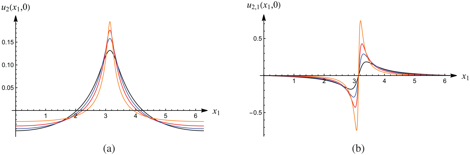
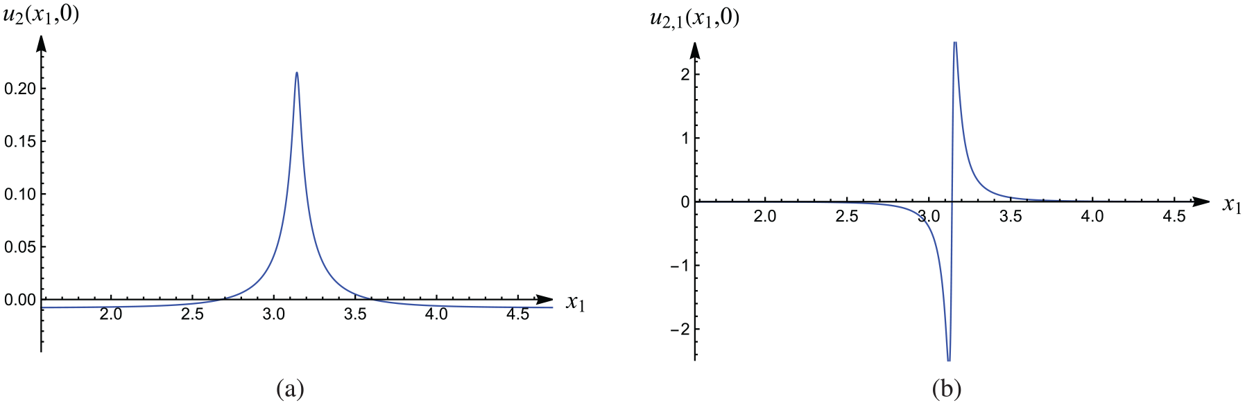
Figure 4 displays the surface elevation and its gradient for $\lambda -{\lambda }_{\mathrm{cr}}=0.001,0.01,0.02,0.04$ , respectively. It is seen that as $\lambda -{\lambda }_{\mathrm{cr}}$ is increased gradually, the surface elevation becomes more and more localized. Figure 5 shows these profiles for the larger value $\lambda -{\lambda }_{\mathrm{cr}}=0.15$ . It is seen that the surface elevation has taken the form of a mountain ridge and is rather like a static solitary wave.

Figure 4.

Surface elevation (a) and gradient of surface elevation (b) when ${\mu }_{\mathrm{f}}/{\mu }_{\mathrm{s}}=5$ , $\nu =0.4999$ , prestretch ${\lambda }_0=0.65$ , and the bilayer width is 200 times the film thickness. The fours curves in each plot correspond to $\lambda -{\lambda }_{\mathrm{cr}}=0.001,0.01,0.02,0.04$ , respectively (Online version in color).

Figure 5.

Surface elevation (a) and gradient of surface elevation (b) when $\lambda -{\lambda }_{\mathrm{cr}}=0.15$ and other parameter values same as in Figure 4. Note that the profiles are shown in the narrower interval $[\pi -\pi /2,\pi +\pi /2]$ to reflect the localizations (Online version in color).

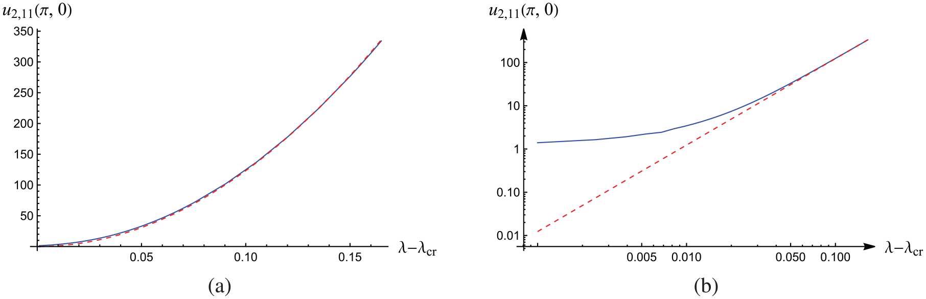
To characterize how the steepness of the profiles at $x_1=\pi$ in Figures 4(b) and 5(b) varies with respect to $\lambda -{\lambda }_{\mathrm{cr}}$ , we show in Figure 6 the dependence of $u_{2,11}(\pi ,0)$ on $\lambda -{\lambda }_{\mathrm{cr}}$ with the other parameters taking the same values as in Figures 4 and 5. Fitting the numerical results (solid line) to the expression $u_{2,11}(\pi ,0)=a(\lambda -{\lambda }_{\mathrm{cr}}{)}^2$ , we find $a=12342$ . It is seen that there is very good agreement between the numerical results and the fitted curve when $\lambda -{\lambda }_{\mathrm{cr}}$ is sufficiently large. This means that the gradient will become infinite only in the limit $\lambda -{\lambda }_{\mathrm{cr}}\to \infty$ . However, in the latter limit, the current weakly nonlinear analysis is no longer valid, and a fully nonlinear analysis is required to describe the further evolution of the surface elevation.

Figure 6.

Dependence of $u_{2,11}(\pi ,0)$ on $(\lambda -{\lambda }_{\mathrm{cr}})$ , showing that the former is proportional to $(\lambda -{\lambda }_{\mathrm{cr}}{)}^2$ for sufficiently large values of $\lambda -{\lambda }_{\mathrm{cr}}$ . The solid curve represents the numerical results whereas the dashed curve is $u_{2,11}(\pi ,0)=a(\lambda -{\lambda }_{\mathrm{cr}}{)}^2$ where $a$ is obtained by fitting the quadratic expression to the numerical results. (a) and (b) display the same information with the only difference that (b) is in log scales.

We may also start with $N=3$ , in which case we obtain a quadratic equation for $B_1^2$ which have real solutions only if

$${\lambda }_s>-c_0/c_1,\mathrm{o}r{\lambda }_s<-s{c}_0/c_1,$$

where

$$s=\frac{3({\mathcal{K}}_{21}^2({\mathcal{K}}_{31}-2{\mathcal{K}}_{32})-2{\mathcal{K}}_{32}^2({\mathcal{K}}_{31}+{\mathcal{K}}_{32}))}{{\mathcal{K}}_{21}^2({\mathcal{K}}_{31}-2{\mathcal{K}}_{32})-6{\mathcal{K}}_{32}^2({\mathcal{K}}_{31}+{\mathcal{K}}_{32})}.$$

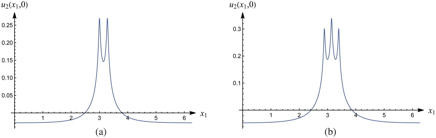
Again, it is found that non-trivial convergent solutions can be found only for ${\lambda }_s>-c_0/c_1$ . In addition to the solution that has already been found by starting from $N=2$ , a second solution is also found in which the profile of $u_2(x_1,0)$ has two local maxima (two humps). Starting with $N=4$ , one more solution with three humps is found in addition to the two found when $N=3$ . The two-hump and three-hump solutions are displayed in Figure 7 for the case when $\lambda -{\lambda }_{\mathrm{cr}}=0.06$ . We may also start with $N=5$ , but in this case the five algebraic equations cannot be solved exactly. We could solve these equations numerically, but this is not explored further. It is very likely that more multi-hump solutions could be found.

Figure 7.

Two-hump (a) and three-hump (b) solutions when $\lambda -{\lambda }_{\mathrm{cr}}=0.1$ .

6. Conclusion

Our study has been motivated by the simulation results given by Cao and Hutchinson [22], where it was shown that when the substrate is subjected to a prestretch equal to 2, a film-substrate bilayer in which the film is much stiffer (with modulus ratio as large as 836) would undergo a secondary bifurcation in the form of a mountain ridge mode. In this article, we have provided a scenario in which a mountain ridge mode (resembling a static solitary wave) may emerge as a first bifurcation. This possibility exists for modulus ratios in the interval ${\mu }_{\mathrm{f}}/{\mu }_{\mathrm{s}}\in (1,7)$ approximately and is only possible if the substrate is pre-compressed.

A typical scenario that the current study addresses is as follows. Suppose that in a numerical simulation or an experimental study we consider a bilayer structure whose width in the $x_1-\mathrm{direction}$ is $2\pi /k$ for some positive number $k$ and whose film has thickness $h$ such that $\mathrm{kh}<<1$ . Suppose that the modulus ratio ${\mu }_{\mathrm{f}}/{\mu }_{\mathrm{s}}$ is 5 and the substrate is first subjected to a prestretch ${\lambda }_0=0.65$ and then the bilayer is compressed together gradually. We wish to know what wrinkling patterns will form on the surface of the bilayer structure.

It is shown in this article that a linear bifurcation analysis predicts that the critical wavenumber is zero. This implies that the wavelength of the wrinkling mode will be as large as the setup allows. If the bilayer is finite in the $x_1-\mathrm{direction}$ as specified above, the buckling mode will be a single hump spanning the entire width $(0,2\pi /k)$ . As $\lambda$ is decreased from the critical value ${\lambda }_{\mathrm{cr}}$ , the single hump will become more and more localized and the surface elevation will become steeper and steeper. This evolution should be observable in numerical simulations, but unlikely to be observable experimentally since the post-buckling solutions are probably unstable. It would be of interest to trace this solution away from the bifurcation point into the fully nonlinear regime to see whether it would join a stable branch. If it does, then the solution on the stable branch would be the solution that the bilayer structure would snap to when it is compressed to the bifurcation point. Thus, it is hoped that our analytical results will provide some guide on future experimental and numerical studies.