Bespoke two-dimensional elasticity and the nonlinear analogue of Cauchy’s relations

Abstract

Is it possible to design an architectured material or structure whose elastic energy is arbitrarily close to a specified continuous function? This is known to be possible in one dimension, up to an additive constant (Dixon et al., Bespoke extensional elasticity through helical lattice systems, Proc. R. Soc. A. (2019)). Here, we explore the situation in two dimensions. Given (1) a continuous energy function $E(C)$ , defined for two-dimensional right Cauchy–Green deformation tensors $C$ contained in some compact set and (2) a tolerance $ϵ>0$ , can we construct a spring-node unit cell (of a lattice) whose energy is approximately $E$ , up to an additive constant, with $L^{\infty }$ -error no more than $ϵ$ ? We show that the answer is yes for affine $E$ s (i.e., for energies $E$ that are quadratic in the deformation gradient), but that the general situation is more subtle and is related to the generalisation of Cauchy’s relations to nonlinear elasticity.

1. Introduction

Architectured materials (or meta-materials) are able to manifest, in the continuum limit, phenomenon not observed in classical elasticity. For example, auxetic materials have a negative Poisson’s ratio (for a review, see, for example, Ren et al. [1]), while traditionally this quantity was required to be positive. Similarly, restrictions on the elastic moduli need to be relaxed in the context of active solids [2, 3]. Materials that arise from topology optimisation have inspired increased sophistication in symmetry classification of elastic moduli [4].

The aforementioned extensions of classical elasticity concern the elastic modulus, and thus materials whose energy is quadratic in the deformation. However, a much more general question can be raised: How much freedom does a designer of an architectured material have if the elastic energy function is the design objective? In particular, can we formulate a design paradigm that is able to attain any desired energy function to specified accuracy?

1.1. One-dimensional extensional elasticity

Dixon et al. [5] addressed this question for one-dimensional extensional elasticity. Two key insights underlie their work. First, they observed that due to the Weierstrass approximation theorem, it suffices to aim to attain polynomial energy functions to specified accuracy. Second, they noticed that the extensional energies of a helical lattice system designed by Pirrera et al. [6] spanned, to sufficient accuracy, the linear space of polynomials, as geometric and material parameters in the design are varied. Combining these two insights, they presented a single design paradigm, namely, helical lattices in parallel, whose extensional energy can be tailored to be arbitrarily close to any given continuous function, up to an additive constant.

In this paper, we extend their result to two-dimensional elasticity.

1.2. Extension to higher dimensions

Let ${\mathrm{R}}_{+}^{2\times 2}$ be the subset of $R^{2\times 2}$ with positive determinant and ${\mathrm{S}}_{+}^{2\times 2}$ be the further subset which is also symmetric. The $L^{\infty }$ norm on continuous functions from ${\mathrm{S}}_{+}^{2\times 2}$ to $\mathbb{R}$ is denoted $\parallel ·{\parallel }_{\infty }$ .

Let $F\in {\mathrm{R}}_{+}^{2\times 2}$ be a deformation gradient and $C=F^{T}F\in {\mathrm{S}}_{+}^{2\times 2}$ be the corresponding right Cauchy–Green deformation tensor.

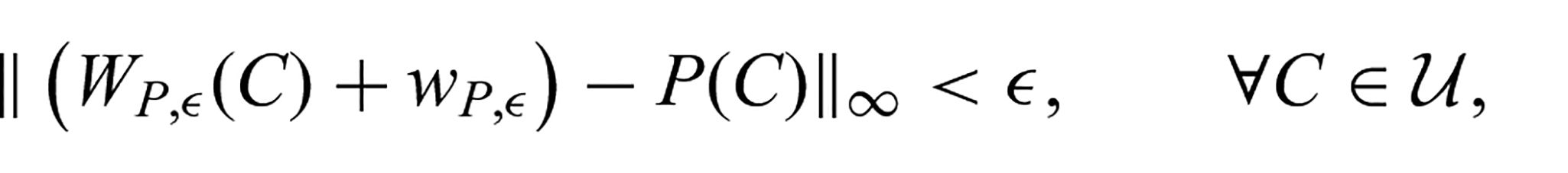
Given a compact $\mathcal{U}\subset {\mathrm{S}}_{+}^{2\times 2}$ , a continuous function $W:\mathcal{U}\to \mathbb{R}$ and a tolerance $ϵ>0$ , we would like to design a two-dimensional structure whose energy $W_{\mathcal{U},ϵ}$ satisfies:

$$\parallel (W_{\mathcal{U},ϵ}(C)+w_{\mathcal{U},ϵ})-W(C){\parallel }_{\infty }<ϵ,\forall C\in \mathcal{U},$$

(1)

for some $w_{\mathcal{U},ϵ}\in \mathbb{R}$ which is independent of $C$ . Note that by phrasing the question in terms of $C$ , rather than $F$ , we have restricted ourselves to frame-invariant functions, both for the energy that we wish to approximate and for the approximate energy.

Drawing inspiration from the one-dimensional result, it is natural to invoke the Stone–Weierstrass Theorem (cf., for example, Simmons [7]). This is a far-reaching generalisation of the Weierstrass approximation theorem, but for our purposes, the following corollary suffices.

Corollary 1. Let $\mathcal{U}\subset {\mathrm{S}}_{+}^{2\times 2}$ be compact, $W:\mathcal{U}\to \mathbb{R}$ be continuous, and $ϵ>0$ . Then, there exists a polynomial $P_{W,\mathcal{U},ϵ}$ in $C$ (to be precise, a trivariate polynomial in the three independent components of $C$ ) such that:

$$\parallel P_{W,\mathcal{U},ϵ}(C)-W(C){\parallel }_{\infty }<\frac{ϵ}{2},\forall C\in \mathcal{U}.$$

(2)

In light of this result, we restrict ourselves to designing structures whose energy $W_{\mathcal{U},ϵ}$ approximates polynomials on compact sets $\mathcal{U}\subset {\mathrm{S}}_{+}^{2\times 2}$ :

$$\parallel (W_{\mathcal{U},ϵ}(C)+w_{\mathcal{U},ϵ})-P_{W,\mathcal{U},ϵ}(C){\parallel }_{\infty }<\frac{ϵ}{2},\forall C\in \mathcal{U},$$

(3)

for some constant $w_{\mathcal{U},ϵ}\in \mathbb{R}$ which is independent of $C$ . Then, equations (2) and (3), together with the triangle inequality, yield equation (1).

A further consideration arises if the said structure forms the unit cell of a lattice. In this case, the continuum energy density need not coincide with the energy of the unit cell. We refer the reader to E and Ming [8] for a further exploration of this issue; here, we focus on the energy of the unit cell.

1.3. The main result

In this paper, we explore the question raised by equation (3): given a (multivariate) polynomial $P$ defined on some compact subset $\mathcal{U}\in {\mathrm{S}}_{+}^{2\times 2}$ and $ϵ>0$ , can we construct a unit cell $L_{P,ϵ}$ whose continuum energy $W_{P,ϵ}$ satisfies:

$$\parallel (W_{P,ϵ}(C)+w_{P,ϵ})-P(C){\parallel }_{\infty }<ϵ,\forall C\in \mathcal{U},$$

for some $w_{P,ϵ}\in \mathbb{R}$ which is independent of $C$ ?

We show that this is indeed possible, with a rectangular lattice, when $P$ has order 0 or 1 (see section 2.1). In other words, we can approximate any frame-invariant polynomial energy which is at most quadratic in $F$ to arbitrary accuracy. Furthermore, unsurprisingly, this can be done via linear springs (i.e., springs whose extensional energy is quadratic in the deformation).

However, for polynomials with higher orders, we need multiple layers of lattices and, even so, succeed only partially (see section 2.2). We provide insight into why the order-one construction does not extend to higher-order polynomials and characterise those polynomials which can be approximated. Our main result is the following.

Theorem 1. Let $\mathcal{U}\subset {\mathrm{S}}_{+}^{2\times 2}$ be compact, and $\mathcal{U}∍C\mapsto P(C)\in ℝ$ be a polynomial of order $N$ which does not intersect the ideals generated by either $C_{11}{C}_{22}$ or $C_{12}^2$ (in other words, $P$ includes no terms which are multiples of either $C_{11}{C}_{22}$ or $C_{12}^2$ ).

Then, there exists a layered rectangular unit cell $L_{P,ϵ}$ , containing no more than $\lceil \frac{N(N+2)}{4}\rceil$ layers, whose elastic energy $W_{P,ϵ}$ satisfies:

$$\parallel (W_{P,ϵ}(C)+w_{P,ϵ})-P(C){\parallel }_{\infty }<ϵ,\forall C\in \mathcal{U},$$

(4)

for some $w_{L_P}\in \mathbb{R}$ which is independent of $C$ .

The restriction that the polynomial $P$ should not intersect the ideals generated by either $C_{11}{C}_{22}$ or $C_{12}^2$ can be understood as a generalisation of Cauchy’s relations to two-dimensional nonlinear elasticity. We address this in section 3 after proving the theorem.

2. Proof of Theorem 1

Our proof proceeds by considering the given polynomial $P$ term by term. Constant and linear terms are considered in section 2.1, quadratic terms in section 2.2, cubic terms in section 2.3, and higher-order terms in section 2.4. We remind the reader that since the polynomial is specified in terms of the right Cauchy–Green deformation tensor $C$ , an energy that is linear in $C$ corresponds to what would normally be called a “quadratic energy,” i.e., quadratic in the deformation gradient $F$ .

The natural numbers (including $0$ ) are denoted $\mathbb{N}$ and the positive reals are denoted ${\mathbb{R}}_{+}$ . The standard orthonormal basis vectors for ${\mathbb{R}}^2$ are $e_1$ and $e_2$ . For the reader’s convenience, we gather together some basic facts about multivariate polynomials in Appendix 1.

For brevity, for $\theta \in \mathbb{R}$ , we set:

$$\begin{array}{c}{c}_{\theta }:=\cos \theta ,\hfill \\ s_{\theta }:=\sin \theta ;\hfill \end{array}$$

and to avoid cluttered notation, for $C\in {\mathrm{S}}_{+}^{2\times 2}$ , we use the shorthand:

$$x:=C_{11},$$

(5a)

$$y:=C_{12},$$

(5b)

$$z:=C_{22}.$$

(5c)

2.1. Bespoke lattices with energy constant or linear in $C$

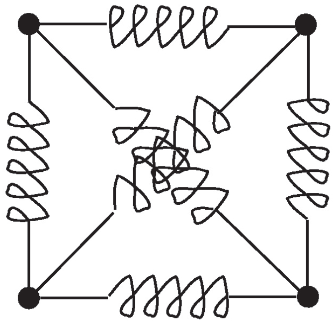
Consider a unit cell, as illustrated in Figure 1. The nodes of this unit cell are connected through one-dimensional elements (“springs”) whose elastic extensional energy functions can be chosen to be arbitrarily close, modulo a constant, to any desired continuous function. There are three kinds of springs, namely, those inclined at angles $0$ , $\frac{\pi }{4}$ and $\frac{\pi }{2}$ to $e_1$ .

Figure 1.

The unit cell of a rectangular lattice. The construction in section 2.1 uses the special case when the rectangle is in fact a square and one diagonal spring is omitted.

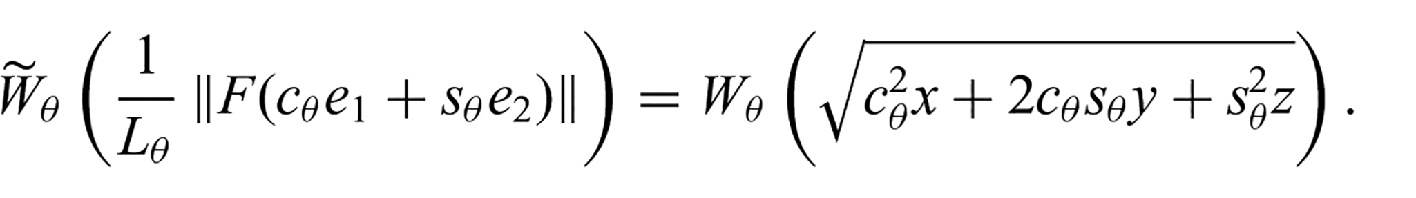
Let $L_{\theta }$ be the rest length of the spring inclined at $\theta$ and ${\tilde{W}}_{\theta }:{\mathbb{R}}_{+}\to \mathbb{R}$ be its extensional energy. When the boundary of this unit cell is subjected to a deformation $F\in {\mathrm{R}}_{+}^{2\times 2}$ , the energy in the spring is:

$${\tilde{W}}_{\theta }(\frac{1}{L_{\theta }}\Vert F(c_{\theta }{e}_1+s_{\theta }{e}_2)\Vert )=W_{\theta }\left(\sqrt{c_{\theta }^{2}x+2c_{\theta }{s}_{\theta }y+s_{\theta }^{2}z}\right).$$

Here, we have used the shorthand from (5) and have absorbed $L_{\theta }$ into the definition of $W_{\theta }$ .

Now, suppose $W_{\theta }$ is—up to an $L^{\infty }(\mathcal{U},\mathbb{R})$ -error at most $\frac{ϵ}{3}$ —either (1) a constant or (2) a monomial of degree $2$ modulo a constant. This is possible from Dixon et al. [5]. Then:

$${\tilde{W}}_{\theta }(\frac{1}{L_{\theta }}\Vert F(c_{\theta }{e}_1+s_{\theta }{e}_2)\Vert )\approx q_{\theta }+r_{\theta }(c_{\theta }^{2}x+2c_{\theta }{s}_{\theta }y+s_{\theta }^{2}z),$$

(6)

for some constants $q_{\theta },r_{\theta }\in \mathbb{R}$ . Note that the polynomial in equation (6) is, up to a constant, a homogeneous linear trinomial in $(x,y,z)$ and also a homogeneous quadratic binomial in $(c_{\theta },s_{\theta })$ . We will return to this observation later.

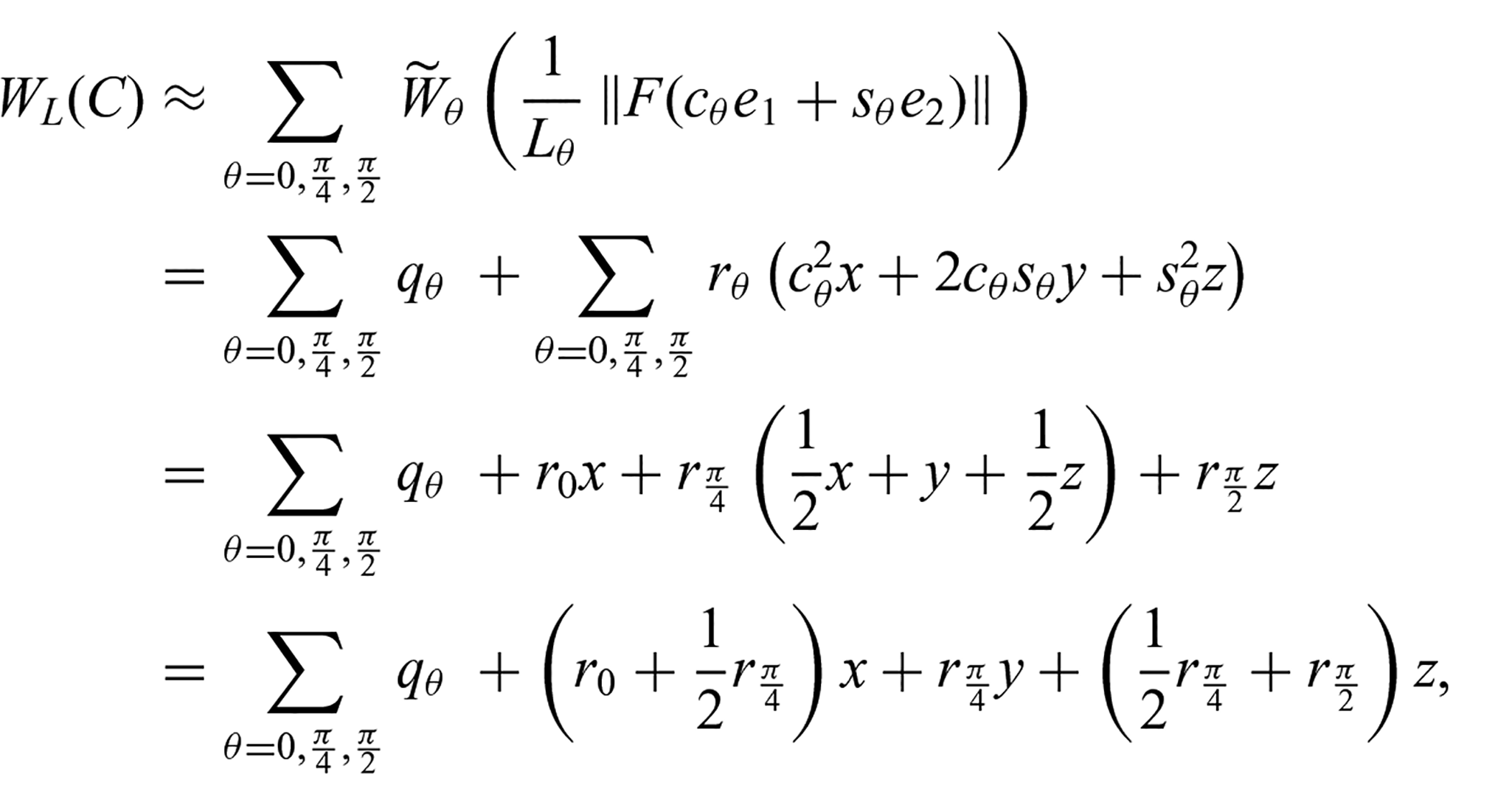
The energy of the unit cell is:

$$\begin{array}{c}{W}_L(C)\approx \sum _{\theta =0,\frac{\pi }{4},\frac{\pi }{2}}{\tilde{W}}_{\theta }(\frac{1}{L_{\theta }}\Vert F(c_{\theta }{e}_1+s_{\theta }{e}_2)\Vert )\hfill \\ =\sum _{\theta =0,\frac{\pi }{4},\frac{\pi }{2}}{q}_{\theta }+\sum _{\theta =0,\frac{\pi }{4},\frac{\pi }{2}}{r}_{\theta }(c_{\theta }^{2}x+2c_{\theta }{s}_{\theta }y+s_{\theta }^{2}z)\hfill \\ =\sum _{\theta =0,\frac{\pi }{4},\frac{\pi }{2}}{q}_{\theta }+r_{0}x+r_{\frac{\pi }{4}}(\frac{1}{2}x+y+\frac{1}{2}z)+r_{\frac{\pi }{2}}z\hfill \\ =\sum _{\theta =0,\frac{\pi }{4},\frac{\pi }{2}}{q}_{\theta }+(r_0+\frac{1}{2}{r}_{\frac{\pi }{4}})x+r_{\frac{\pi }{4}}y+(\frac{1}{2}{r}_{\frac{\pi }{4}}+r_{\frac{\pi }{2}})z,\hfill \end{array}$$

and the $L^{\infty }(\mathcal{U},\mathbb{R})$ -error is at most $ϵ$ .

Thus, given any trivariate polynomial of order 1 up to a constant, say:

$$P(C)=p_0+p_{11}{C}_{11}+p_{12}{C}_{12}+p_{22}{C}_{22}\equiv p_0+p_{11}x+p_{12}y+p_{22}z,$$

it suffices to design the energies of the three springs such that $r_{\frac{\pi }{4}}$ is sufficiently close to $c_{12}$ , and then $r_0+\frac{1}{2}{r}_{\frac{\pi }{4}}$ and $\frac{1}{2}{r}_{\frac{\pi }{4}}+r_{\frac{\pi }{2}}$ sufficiently close to $c_{11}$ and $c_{22}$ , respectively. The one-dimensional result in [5] guarantees that this is possible. Equation (4) is then satisfied.

Remark 1. The construction above explains why our results do not contradict the well-known result due to Cauchy (see Love [9]) that lattice systems with central force potentials necessarily have a Poisson’s ratio of $\frac{1}{4}$ in the linearised continuum limit. That result assumes that all springs in the lattice have the same extensional energy function. Our construction relies on the availability of up to three kinds of springs.

2.2. Bespoke lattices with energy quadratic in $C$

Let us now see if we can replicate the construction in section 2.1 to design a unit cell whose energy is a given quadratic function of $C$ , modulo a constant and up to an $L^{\infty }(\mathcal{U},\mathbb{R})$ -error at most $ϵ$ .

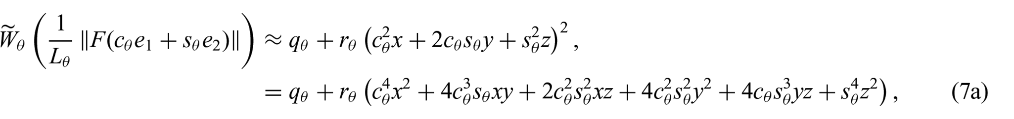
We proceed as in section 2.1, but choose $W_{\theta }$ to be a monomial of degree $4$ , modulo a constant and up to an $L^{\infty }(\mathcal{U},\mathbb{R})$ -error at most $\frac{ϵ}{5}$ . Then, equation (6) becomes:

$$\begin{array}{c}{\tilde{W}}_{\theta }(\frac{1}{L_{\theta }}\Vert F(c_{\theta }{e}_1+s_{\theta }{e}_2)\Vert )\approx q_{\theta }+r_{\theta }{(c_{\theta }^{2}x+2c_{\theta }{s}_{\theta }y+s_{\theta }^{2}z)}^2,\hfill \\ =q_{\theta }+r_{\theta }(c_{\theta }^4{x}^2+4c_{\theta }^3{s}_{\theta }\mathrm{xy}+2c_{\theta }^2{s}_{\theta }^2\mathrm{xz}+4c_{\theta }^2{s}_{\theta }^2{y}^2+4c_{\theta }{s}_{\theta }^3\mathrm{yz}+s_{\theta }^4{z}^2),\hfill \end{array}$$

(7a)

for some $q_{\theta },r_{\theta }\in \mathbb{R}$ . Similar to equation (6), the expression in equation (7a) is, up to a constant, a homogeneous quadratic trinomial in $(x,y,z)$ and also a homogeneous quartic binomial in $(c_{\theta },s_{\theta })$ .

The linear space of quadratic trinomials is six-dimensional, as can be seen from the six terms in equation (7a). Thus, to approximate an arbitrary quadratic (in $C$ ) elastic energy, we need six linearly independent polynomials of the form (7a). These would have to be generated by six distinct choices of $\theta$ .

Unfortunately, this is not possible since the coefficients of $\mathrm{xz}$ and $y^2$ are not independent: the latter is always twice the former. This can also be seen from the coefficient of $c_{\theta }^2{s}_{\theta }^2$ when the expression in equation (7a) is written as a binomial in $(c_{\theta },s_{\theta })$ :

$${\tilde{W}}_{\theta }(\frac{1}{L_{\theta }}\Vert F(c_{\theta }{e}_1+s_{\theta }{e}_2)\Vert )\approx q_{\theta }+r_{\theta }(x^2{c}_{\theta }^4+4{\mathrm{xyc}}_{\theta }^3{s}_{\theta }+2(\mathrm{xz}+2y^2)c_{\theta }^2{s}_{\theta }^2+4\mathrm{yz}{c}_{\theta }{s}_{\theta }^3+z^2{s}_{\theta }^4).$$

(7b)

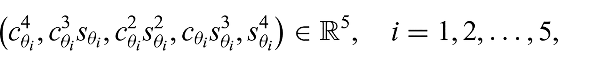
However, the five-dimensional subspace that satisfies this constraint can be achieved by five distinct choices of $\theta$ . This follows from the following lemma.

Lemma 1. Let ${\theta }_1,{\theta }_2,\dots ,{\theta }_5\in [0,\pi )\backslash \frac{\pi }{2}$ be distinct. Then, the five vectors:

$$(c_{{\theta }_i}^4,c_{{\theta }_i}^3{s}_{{\theta }_i},c_{{\theta }_i}^2{s}_{{\theta }_i}^2,c_{{\theta }_i}{s}_{{\theta }_i}^3,s_{{\theta }_i}^4)\in {\mathbb{R}}^5,i=1,2,\dots ,5,$$

are linearly independent.

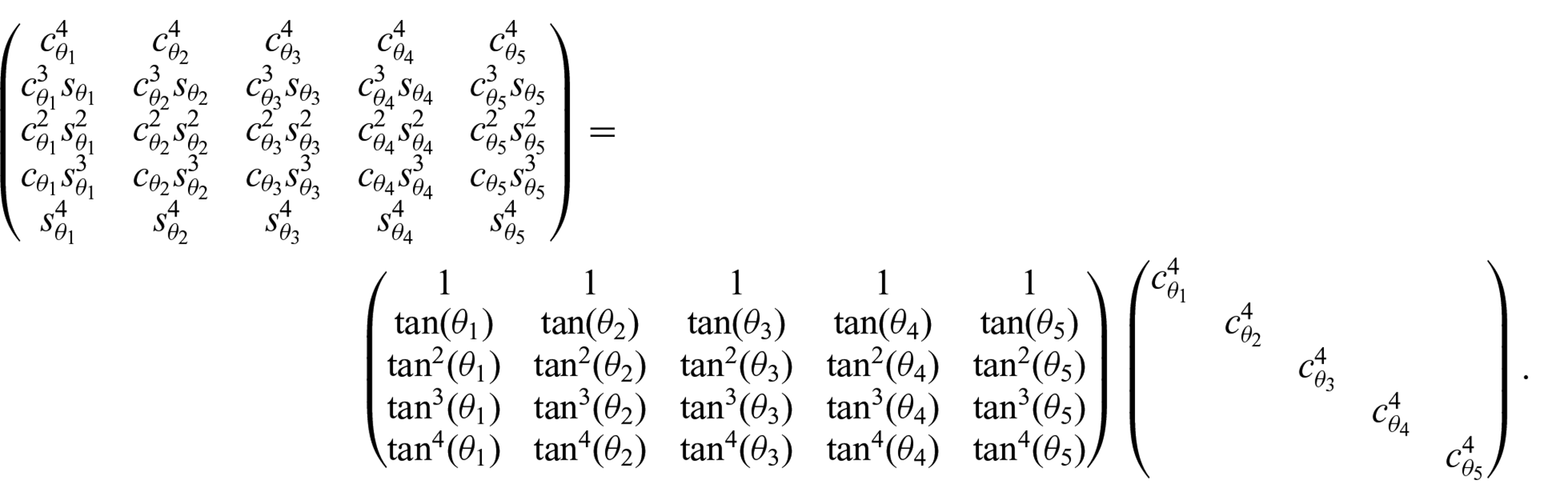
Proof. By a simple calculation:

$$\begin{array}{c}\left(\begin{array}{ccccc}{c}_{{\theta }_1}^4\hfill & c_{{\theta }_2}^4\hfill & c_{{\theta }_3}^4\hfill & c_{{\theta }_4}^4\hfill & c_{{\theta }_5}^4\hfill \\ \multicolumn{1}{c}{c_{{\theta }_1}^3{s}_{{\theta }_1}}& c_{{\theta }_2}^3{s}_{{\theta }_2}\hfill & c_{{\theta }_3}^3{s}_{{\theta }_3}\hfill & c_{{\theta }_4}^3{s}_{{\theta }_4}\hfill & c_{{\theta }_5}^3{s}_{{\theta }_5}\hfill \\ \multicolumn{1}{c}{c_{{\theta }_1}^2{s}_{{\theta }_1}^2}& c_{{\theta }_2}^2{s}_{{\theta }_2}^2\hfill & c_{{\theta }_3}^2{s}_{{\theta }_3}^2\hfill & c_{{\theta }_4}^2{s}_{{\theta }_4}^2\hfill & c_{{\theta }_5}^2{s}_{{\theta }_5}^2\hfill \\ \multicolumn{1}{c}{c_{{\theta }_1}{s}_{{\theta }_1}^3}& c_{{\theta }_2}{s}_{{\theta }_2}^3\hfill & c_{{\theta }_3}{s}_{{\theta }_3}^3\hfill & c_{{\theta }_4}{s}_{{\theta }_4}^3\hfill & c_{{\theta }_5}{s}_{{\theta }_5}^3\hfill \\ \multicolumn{1}{c}{s_{{\theta }_1}^4}& s_{{\theta }_2}^4\hfill & s_{{\theta }_3}^4\hfill & s_{{\theta }_4}^4\hfill & s_{{\theta }_5}^4\hfill \end{array}\right)=\hfill \\ \left(\begin{array}{ccccc}1\hfill & 1\hfill & 1\hfill & 1\hfill & 1\hfill \\ \multicolumn{1}{c}{\tan ({\theta }_1)}& \tan ({\theta }_2)\hfill & \tan ({\theta }_3)\hfill & \tan ({\theta }_4)\hfill & \tan ({\theta }_5)\hfill \\ \multicolumn{1}{c}{\stackrel{2}{\tan }({\theta }_1)}& \stackrel{2}{\tan }({\theta }_2)\hfill & \stackrel{2}{\tan }({\theta }_3)\hfill & \stackrel{2}{\tan }({\theta }_4)\hfill & \stackrel{2}{\tan }({\theta }_5)\hfill \\ \multicolumn{1}{c}{\stackrel{3}{\tan }({\theta }_1)}& \stackrel{3}{\tan }({\theta }_2)\hfill & \stackrel{3}{\tan }({\theta }_3)\hfill & \stackrel{3}{\tan }({\theta }_4)\hfill & \stackrel{3}{\tan }({\theta }_5)\hfill \\ \multicolumn{1}{c}{\stackrel{4}{\tan }({\theta }_1)}& \stackrel{4}{\tan }({\theta }_2)\hfill & \stackrel{4}{\tan }({\theta }_3)\hfill & \stackrel{4}{\tan }({\theta }_4)\hfill & \stackrel{4}{\tan }({\theta }_5)\hfill \end{array}\right)\left(\begin{array}{ccccc}{c}_{{\theta }_1}^4\hfill & \hfill & \hfill & \hfill & \hfill \\ \hfill & c_{{\theta }_2}^4\hfill & \hfill & \hfill & \hfill \\ \hfill & \hfill & c_{{\theta }_3}^4\hfill & \hfill & \hfill \\ \hfill & \hfill & \hfill & c_{{\theta }_4}^4\hfill & \hfill \\ \hfill & \hfill & \hfill & \hfill & c_{{\theta }_5}^4\hfill \end{array}\right).\hfill \end{array}$$

On the right-hand side, the second matrix is invertible since ${\theta }_i\ne \frac{\pi }{2}$ . In the first matrix, all components are finite for the same reason. This matrix is a Vandermonde matrix and thus is invertible when the $\theta$ s are distinct (cf., for example, Prasolov [10]). We conclude that the five columns of the matrix on the left-hand side are linearly independent. □

Note that this lemma does not exclude the choice of $\frac{\pi }{2}$ as one of the $\theta$ s.

Thus, we can approximate any energy which lies in the span of $\{x^2,\mathrm{xy},\mathrm{xz}+2y^2,\mathrm{yz},z^2\}$ , but an energy which is non-zero on the subspace spanned by $\mathrm{xz}-\frac{1}{2}{y}^2$ is not approximable. In particular:

$$\mathrm{Span}\{\mathrm{xz},y^2\},$$

(8)

is only partially approximable.

The corresponding construction would generically need five springs but a rectangular unit with diagonal springs, illustrated in Figure 1, can accommodate at most four springs. This obstacle can be overcome using two layers of rectangular lattices which are coupled at the boundary.

2.3. Bespoke lattices with energy cubic in $C$

Before we consider the general case, it is instructive, as a last explicit example, to analyse to what extent it is possible to design a lattice whose energy is a given cubic function of $C$ , modulo a constant and up to an $L^{\infty }(\mathcal{U},\mathbb{R})$ -error at most $ϵ$ .

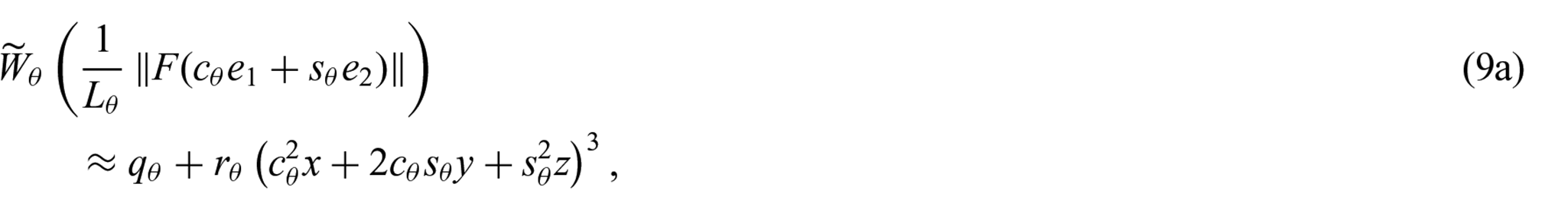
We proceed as in section 2.1, but choose $W_{\theta }$ to be a monomial of degree $6$ , modulo a constant and up to an $L^{\infty }(\mathcal{U},\mathbb{R})$ -error at most $\frac{ϵ}{7}$ . Then, equation (6) becomes:

$$\begin{array}{c}{\tilde{W}}_{\theta }(\frac{1}{L_{\theta }}\Vert F(c_{\theta }{e}_1+s_{\theta }{e}_2)\Vert )\hfill \\ \approx q_{\theta }+r_{\theta }{(c_{\theta }^{2}x+2c_{\theta }{s}_{\theta }y+s_{\theta }^{2}z)}^3,\hfill \end{array}$$

(9a)

$$=q_{\theta }+r_{\theta }\left(\begin{array}{c}{c}_{\theta }^6{x}^3+6c_{\theta }^5{s}_{\theta }{x}^{2}y+3c_{\theta }^4{s}_{\theta }^2{x}^{2}z+12c_{\theta }^4{s}_{\theta }^{2}x{y}^2+12c_{\theta }^3{s}_{\theta }^3\mathrm{xyz}\hfill \\ \multicolumn{1}{c}{+3c_{\theta }^2{s}_{\theta }^{4}x{z}^2+8c_{\theta }^3{s}_{\theta }^3{y}^3+12c_{\theta }^2{s}_{\theta }^4{y}^{2}z+6c_{\theta }{s}_{\theta }^{5}y{z}^2+s_{\theta }^6{z}^3}\end{array}\right),$$

(9b)

$$=q_{\theta }+r_{\theta }\left(\begin{array}{c}{x}^3{c}_{\theta }^6+6x^2{\mathrm{yc}}_{\theta }^5{s}_{\theta }+3(x^{2}z+4x{y}^2)c_{\theta }^4{s}_{\theta }^2\hfill \\ +4(3\mathrm{xyz}+2y^3)c_{\theta }^3{s}_{\theta }^3+3(x{z}^2+4y^{2}z)c_{\theta }^2{s}_{\theta }^4+6c_{\theta }{s}_{\theta }^{5}y{z}^2+s_{\theta }^6{z}^3\hfill \end{array}\right),$$

(9c)

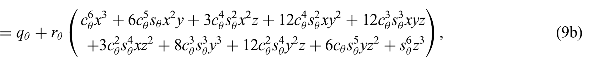
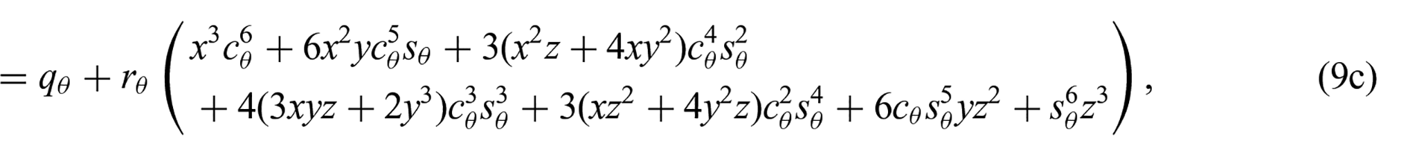
for some $q_{\theta },r_{\theta }\in \mathbb{R}$ . Similar to equation (7), the expression in equation (9b) is a homogeneous cubic trinomial in $(x,y,z)$ and the expression in equation (9c) is a homogeneous hexic binomial in $(c_{\theta },s_{\theta })$ .

The linear space of cubic trinomials is 10-dimensional, as can be seen from the 10 terms in equation (9b). However, only a seven-dimensional subspace can be approximated. The three subspaces which cannot be fully approximated can be read off from equation (9c). They are contained in:

$$\mathrm{Span}\{x^{2}z,x{y}^2\},\mathrm{Span}\{\mathrm{xyz},y^3\},\mathrm{Span}\{x{z}^2,y^{2}z\}.$$

(10)

We see that the six monomials that appear in equation (10) are precisely the cubic monomials which have the quadratic monomials in equation (8) as factors.

However, by choosing seven distinct ${\theta }_i\in [0,\pi )$ , we can approximate any energy that lies in:

$$\mathrm{Span}\{x^3,x^{2}y,x^{2}z+4x{y}^2,3\mathrm{xyz}+2y^3,x{z}^2+4y^{2}z,y{z}^2,z^3\}.$$

This follows from the seven-dimensional analogue of Lemma 1. As before we would need two layers of rectangular lattices which are coupled at the boundary.

2.4. Bespoke lattices with energy of power $m$ in $C$

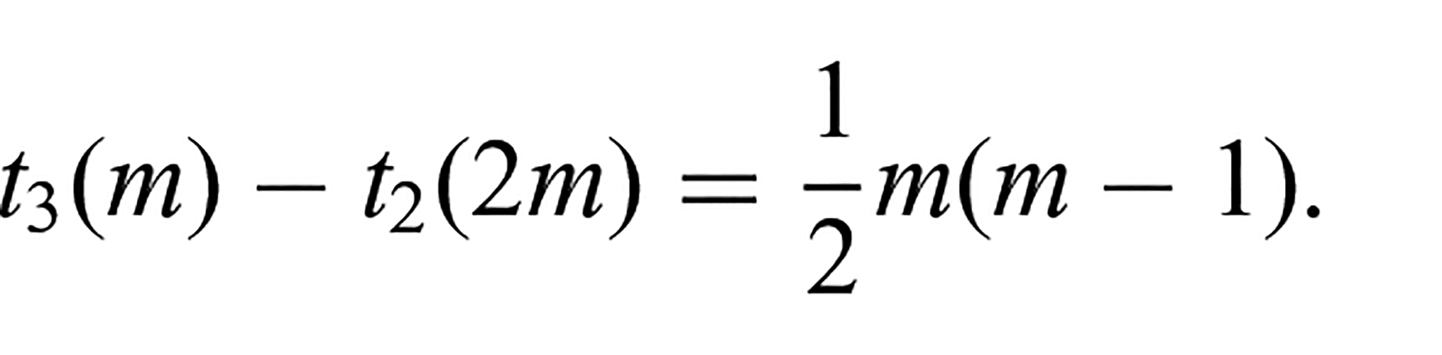
The general case now follows: for $m\in \mathbb{N}$ , there are $t_3(m)$ linearly independent (trivariate) monomials of order $m$ (see section “Trivariate polynomials” in Appendix 1) but only $t_2(2m)$ (see section “Bivariate polynomials” in Appendix 1) can be spanned by the springs in our construction. Thus, the dimension of the subspace of order $m$ that is unapproximable is:

$$t_3(m)-t_2(2m)=\frac{1}{2}m(m-1).$$

Note that this is exactly $t_3(m-2)$ . Thus, we can characterise the subspaces that are only partially approximable.

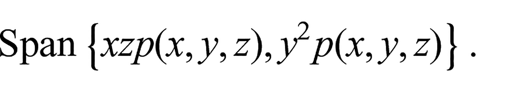
Corollary 2. Let $m\ge 2$ . For every monomial $p(x,y,z)$ of order $m-2$ , the construction above can approximate the energy in (and only in) a one-dimensional subspace of the two-dimensional subspace:

$$\mathrm{Span}\{\mathrm{xzp}(x,y,z),y^{2}p(x,y,z)\}.$$

Thus, when $m=2$ , we obtain equation (8) and when $m=3$ , we obtain equation (10).

It follows that we can approximate any polynomial that vanishes on the union of the ideals generated by $\mathrm{xz}$ and $y^2$ :

Remark 2. Let $P$ be a set of monomials (in $x,y,z$ ) of order $m$ , none of which is a multiple of either $\mathrm{xz}$ or $y^2$ . Then, the construction above can approximate the energy on $\mathrm{Span}\left\{P\right\}$ .

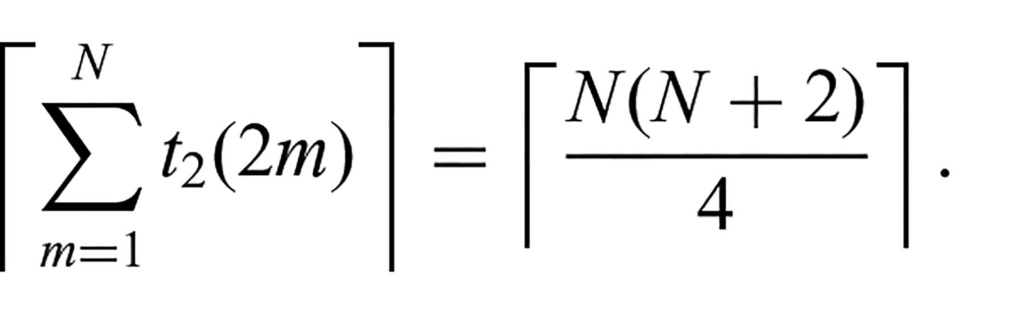
Finally, we can bound the total number of layers of rectangular unit cells needed to approximate a polynomial energy of order $N>0$ , modulo a constant. This is given by:

$$\lceil \sum _{m=1}^N{t}_2(2m)\rceil =\lceil \frac{N(N+2)}{4}\rceil .$$

This completes the proof of Theorem 1.

3. Link to Cauchy’s relations

In linearised elasticity, the elastic modulus $\mathrm{C}$ is required to satisfy the major symmetry:

$${\mathrm{C}}_{\mathrm{ijkl}}={\mathrm{C}}_{\mathrm{klij}},$$

(11a)

and minor symmetries:

$${\mathrm{C}}_{\mathrm{ijkl}}={\mathrm{C}}_{\mathrm{jikl}}={\mathrm{C}}_{\mathrm{ijlk}}.$$

(11b)

If, in addition, the elasticity is postulated to arise from pair potentials between particles—with the potential being independent of the pair of particles—then the further symmetry:

$${\mathrm{C}}_{\mathrm{ijkl}}={\mathrm{C}}_{\mathrm{ikjl}},$$

(11c)

is imposed on $\mathrm{C}$ (see Love [9]). Those relations in equation (11c) that are not part of equation (11a) or (11b) are known as Cauchy’s relations. It is easy to check that in two dimensions, there is only one of them:

$${\mathrm{C}}_{1122}={\mathrm{C}}_{1212}.$$

(11d)

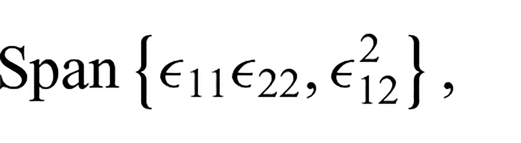
Consider what equation (11d) implies for the elastic energy. Since we are in the realm of linearised elasticity, the elastic energy is a quadratic function of the three independent components of the linearised strain, ${ϵ}_{11}$ , ${ϵ}_{12}$ , and ${ϵ}_{22}$ . The relation (11d) imposes the requirement that, in the quadratic expression for the energy, the coefficient of ${ϵ}_{11}{ϵ}_{22}$ is identical to that of ${ϵ}_{12}^2$ , and thus, the energy on:

$$\mathrm{Span}\{{ϵ}_{11}{ϵ}_{22},{ϵ}_{12}^2\},$$

cannot be arbitrary. Comparing with section 2.2, especially equation (8), we see that this is analogous to the restriction on the terms quadratic in $C$ therein. The cubic analogue is equation (10).

Thus, Corollary 2, which presents the general situation, may be thought of as a generalisation of Cauchy’s relations to nonlinear elasticity, with the further generalisation that we no longer assume that a single potential applies to every pair of particles.

4. Conclusion

The generalisation of Cauchy’s relations presented here is phrased, not directly in terms of the elastic energy, but rather indirectly through the polynomials that approximate the energy. This is natural in that we have approached continuous functions via their polynomial approximations on compact sets. To be precise, for $\mathcal{U}\subset {\mathrm{S}}_{+}^{2\times 2}$ compact, let ${\mathcal{P}}_{\mathcal{U}}$ be the set of polynomials in $(C_{11},C_{12},C_{22})$ which do not intersect the ideals formed by either $C_{11}{C}_{22}$ or $C_{12}^2$ . Moreover, let $\overline{{\mathcal{P}}_{\mathcal{U}}}$ be the closure of ${\mathcal{P}}_{\mathcal{U}}$ in $\parallel ·{\parallel }_{\infty }$ . Then, $\overline{{\mathcal{P}}_{\mathcal{U}}}$ is the set of elastic energies, defined on $\mathcal{U}$ , which satisfy the generalised Cauchy’s relations presented here.

Although it would be convenient for applications, we are unaware of a simpler characterisation of $\overline{{\mathcal{P}}_{\mathcal{U}}}$ . Note also $\overline{{\mathcal{P}}_{\mathcal{U}}}$ depends on $U$ leaving open the possibility that the same expression for the energy might satisfy the generalised Cauchy’s relations on one domain but not on another.

This work also shows that continuum elastic energies not contained in $\overline{{\mathcal{P}}_{\mathcal{U}}}$ cannot arise from pair potentials, not even non-uniform pair potentials. Thus, it provides a test by which a modeller can determine whether a microscopic model with pair potentials could generate a given continuum elastic energy. Such a test would be valid even in contexts far removed from architectured materials, e.g., soft elasticity of biomaterials.

In closing, we expect analogous results to hold in three dimensions. Details will be presented in a subsequent work.