
Abstract
The Euler–Bernoulli beam bending theory in engineering mechanics assumes that the material behavior is isotropic elastic and that plane cross sections remain plane and rigid. It is well-known that this theory suffers from inconsistencies that, e.g., the shear strain is always vanishing, whereas the shear stress does not vanish. In recent work, consistent Euler–Bernoulli beam theories in classical and explicit gradient elasticities were accomplished by assuming the constitutive response to be anisotropic elastic, subject to internal constraints. This approach is extended in the present paper to get consistent Euler–Bernoulli beam theory for gradient elasticity based on Laplacians of stress and strain. The developed beam theory is employed to discuss bending of cantilever beams.
Keywords
1. Introduction
Bending of beams is of fundamental importance, e.g., in engineering mechanics, structural analysis, experimental, and computational mechanics. In the past decades, special attention has been devoted to applications in micro- and macro-electromechanical systems (see, e.g., the review work Thai et al. [1]). It is generally accepted that size effects are essential in the material response of small-scale structural elements as, e.g., beams and plates. Experimental evidence is provided, among others, in Lam et al. [2], Farland and Colton [3] and Liebold and Müller [4]. Common elasticity theories, which allow capturing size effects in the material response, are the micropolar, the micromorphic, the gradient and the nonlocal elasticity. There is considerable amount of works concerning bending of beams, which are formulated in the framework of these non-classical elasticity theories. Of interest for our paper are, among others, the works of Papargyri-Beskou et al. [5], Lam et al. [2], Park and Gao [6], Ma et al. [7], Li et al. [8], Kong et al. [9], Lazopoulos and Lazopoulos [10], Reddy [11], Akgöz and Civalek [12], Xu and Shen [13], Li and Batra [14], Liang et al. [15], Ansari et al. [16], Liang et al. [15], Sherafatnia et al. [17], Yaghoubi et al. [18], Dehrouyeh-Semnani et al. [19], Ebrahimi et al. [20], Niiranen et al. [21], and Shaat et al. [22].
Simple Models of gradient elasticity are very attractive, since they deal with symmetric Cauchy stresses and only a few additional material parameters are usually needed in comparison to classical elasticity. Here, we consider models, which are expressed in terms of Laplacians of the stress and the strain tensors and which may be imagined as generalizations of the classical elasticity law

Particular simple models of explicit and implicit gradient elasticity are, respectively, the laws

and

In these equations,
Implicit gradient elasticity laws of the form (3) are increasingly interpreted as particular cases of Eringen’s non-local elasticity (see, e.g., Yan et al. [30], Xu et al. [31], Ceballes et al. [32], Lim et al. [33], and the references cited there). In general, Eringen’s nonlocal elasticity theory is often used in order to model bending of beams (see, e.g., Eltaher et al. [34], Fernández-Sáez et al. [35], Koutsoumaris et al. [36], Pisano et al. [37], Shaat et al. [38], Thai et al. [1] and the references cited there). A different way to approach model (3) is proposed by Broese et al. [29]. These authors proved that, on one hand, model (3) can be obtained as particular case of Mindlin’s micro-structured elasticity (equivalently Eringen’s micromorphic elasticity). On the other hand, using non-classical thermodynamics, they established an analogy between equation (3) and the three-parameter-Solids of linear viscoelasticity. (The abbreviation 3-PG-Model in equation (3) stands for Three-Parameter-Gradient elasticity model). As elucidated in Broese et al. [29], on the level of mechanical systems the analogy becomes visible by replacing the dashpot element in viscoelasticity by a non-standard spring in gradient elasticity. On the analytical level the analogy arises by replacing the time derivatives in viscoelasticity by Laplacian derivatives in gradient elasticity. It is also emphasized in Broese et al. [29], that in contrast to the Three-Parameter viscoelastic solid, its gradient counterpart allows energy to be stored in all three springs and it does not allow energy to be dissipated. Therefore, the analogy is a formal mathematical and not a physical one.
The Euler–Bernoulli bending theory of beams in elementary mechanics supposes the material behavior to be isotropic elastic. Furthermore, it assumes that the plane cross sections of the beam remain plane and perpendicular to the deformed beam-axis and that the shape of the cross sections does not change (see, e.g., Bauchau and Craig [[39], sections 5.1 and 5.4.2] or Reddy [40]). That means that cross sections undergo rigid body motions. Unfortunately, this theory suffers from the well-known inconsistency that the strain state according to these assumptions implies, e.g., vanishing shear stress always, which is in contradiction with the equilibrium equations in local form. There are other formulations of Euler–Bernoulli beams, which do not assume the cross section to be rigid, but suffer from similar inconsistencies. Such inconsistencies are accepted by interpreting these to be negligible (see, e.g., Bauchau and Craig [[39], section 5.4.2] and Janecka et al. [41]). Almost all Euler–Bernoulli bending theories of beams in gradient elasticity are inconsistent, or they are formulated on the basis of one-dimensional variational principles, so that such theories deal only with section forces.
A consistent Euler–Bernoulli bending theory of beams, for the classical elasticity law (1) and the gradient elasticity law (2), is proposed in Sideris and Tsakmakis [42] and Broese et al. [43]. The inconsistency is removed by assuming the material response to be transverse isotropic subject to internal constraints. It is shown, that all results of the engineering mechanics approach remain valid also in the framework of the consistent formulation. Furthermore, in the case of the gradient elasticity model (2), the consistent formulation offers the possibility to determine distributions of stress components. In the present paper, this consistent Euler–Bernoulli approach is extended to cover the 3-PG-Model in equation (3). The resulting beam theory is employed to discuss bending of cantilever beams. The predicted responses are compared with those according to the consistent formulations of classical elasticity (1) and KG-Model (2). Hence, the aim of the paper is purely theoretical and in particular description of the behavior of specific real materials is not provided.
2. Notation
Only static problems are considered and the deformations are assumed to be small, so we do not distinguish, as usually done, between reference and actual configuration. Unless explicitly stated, all indices will have the range of integers (1,2,3), while summation over repeated indices is implied. All tensorial components are referred to a Cartesian coordinate system
Let

The gradient and the divergence operators are indicated by

Thus, for the Laplacian

Let

3. Fundamental equations, concomitant boundary conditions
It has been mentioned in the introduction that the 3-PG-Model may be considered as a particular case of micromorphic elasticity or as counterpart of the Three-Parameter-Solid of linear viscoelasticity. According to this second approach, the 3-PG-Model has to be viewed as constitutive law and the associated boundary conditions as constitutive boundary conditions. In the following, we shall adopt the second interpretation. In any case, the main equations may be summarized as follows (see Broese et al. [29, 44]).
Field and constitutive equations:


where


In these equations,

Equation (8) represents classical equilibrium equations in the absence of body forces, while equations (9)–(13) are viewed as constitutive equations, which lead to the 3-PG-Model (3) (see Broese et al. [29]).
Boundary conditions:


must be prescribed on
Note that a micromorphic continuum with symmetric micro-deformation tensor
4. Consistent Euler–Bernoulli beam bending theory for the 3-PG-Model
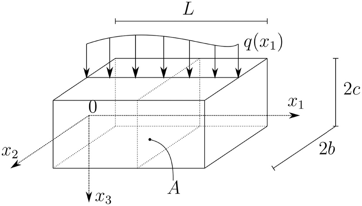
Consider the rectangular beam shown in Figure 1, which has length
ReYoung’s moduli th
It has been remarked in Sideris and Tsakmakis [42], that the Euler–Bernoulli assumptions (cf. Section 1) suggest some kind of anisotropic material response. Actually, assuming transverse isotropic elastic material behavior, subject to internal constraints, these authors established consistent Euler–Bernoulli beam theories for classical and explicit gradient elasticity. This approach will now be used for the 3-PG-Model.
4.1. Transverse isotropic 3-PG-Model with internal constraints
As remarked in Sideris and Tsakmakis [42], vanishing external load in


The Euler–Bernoulli assumption, that cross sections are rigid, suggests infinitely large value

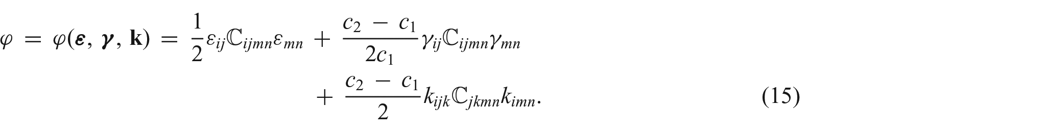
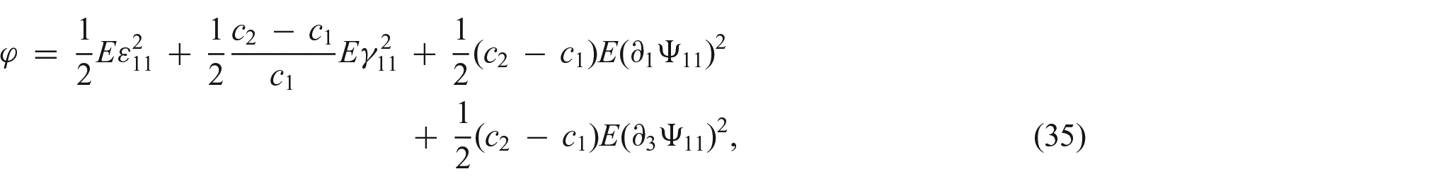
in order for the free energy
Another assumption in the Euler–Bernoulli beam theory is that the cross section remains plane after deformation. Thus, there exist axial displacement

must hold, in order for


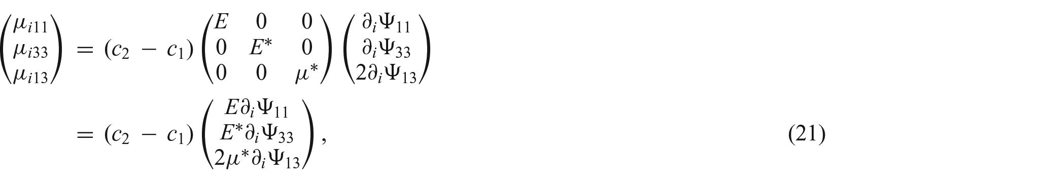
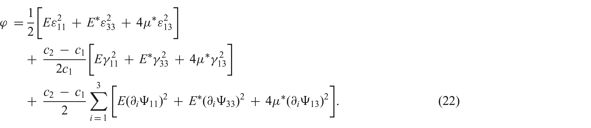
from equations (19)–(22) we find that


and the field equations (8) and (9) reduce to


In an interesting paper, Shaat et al. [22] proposed a micromorphic beam theory with symmetric micro-deformation. Their component
Generally, it is not possible to solve analytically the field equations (36)–(40) and to satisfy given boundary conditions (17) and (18). Therefore, Euler–Bernoulli beam theories simplify the mathematical problem by solving a reduced form of these equations, expressed in terms of section and resulting forces. Such theories reduce the three-dimensional material body to one-dimensional continuum along the
4.2. Virtual work principle—standard formulation
Virtual work principles in statics require for the virtual work of the external forces to be equal to the virtual work of the internal forces. We shall determine the virtual work of the external and the internal forces in sections 4.2.1 and 4.2.2, respectively.
4.2.1. Virtual work of external forces
Generally, virtual work principles in elasticity offer the possibility to derive, besides the equilibrium equations and the boundary conditions, also the elasticity law. However, in order to make comprehensible basic features of the traction component
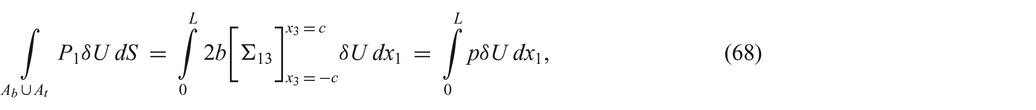
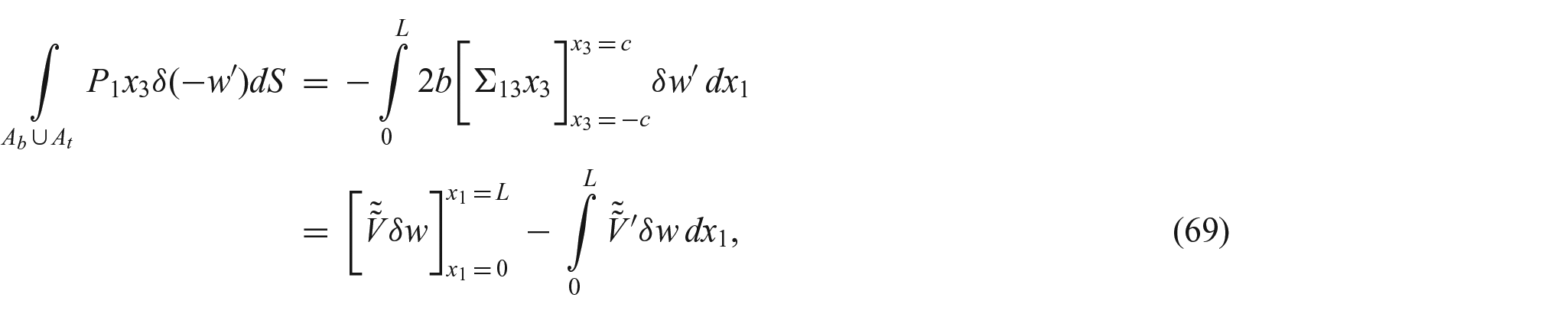
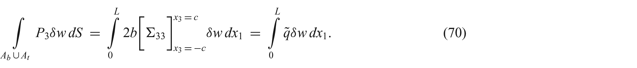
With regard to the boundary conditions (17), (18) and Figure 1, the virtual work of external forces,
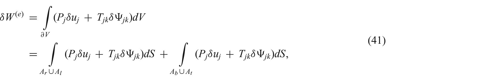
where


By invoking the constitutive laws (30)–(32), we obtain the sectional elasticity laws


where

As we shall see below, the section force
We shall determine first the part of


All other components of
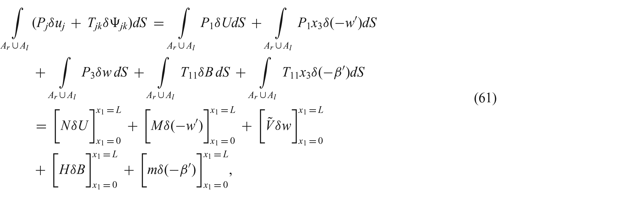
where the definitions (42)–(48) have been used.
When calculating the virtual work expended by


It follows that
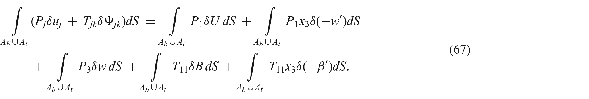
For the first three integrals on the right-hand side of equation (67) we find, with the help of equations (62), (63), (42)–(48) and by using partial integration, that
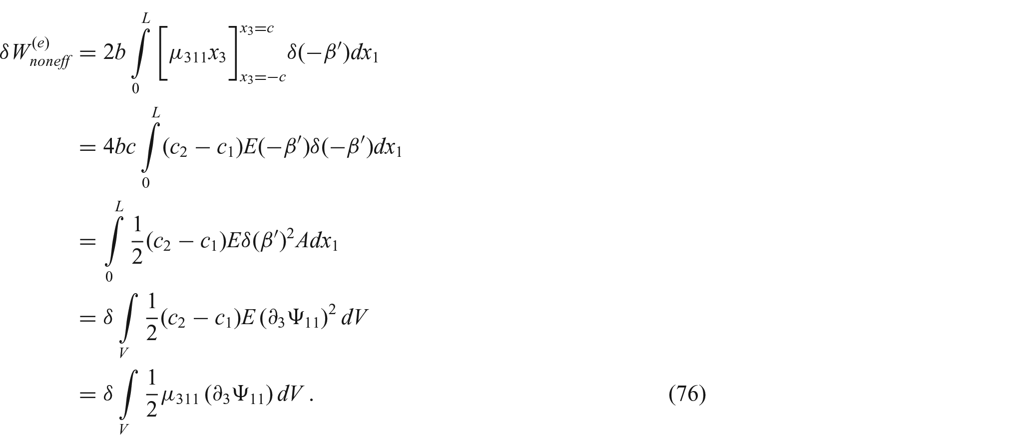
The last two integrals on the right-hand side of equation (67) include the traction

It is worth noticing that

That

An immediate consequence of the last equation is that, the first integral of equation (72) vanishes,

Thus,

and by virtue of equations (71), (21), (27)1, and (33),
It follows from equations (67)–(70), (47) and (72) that
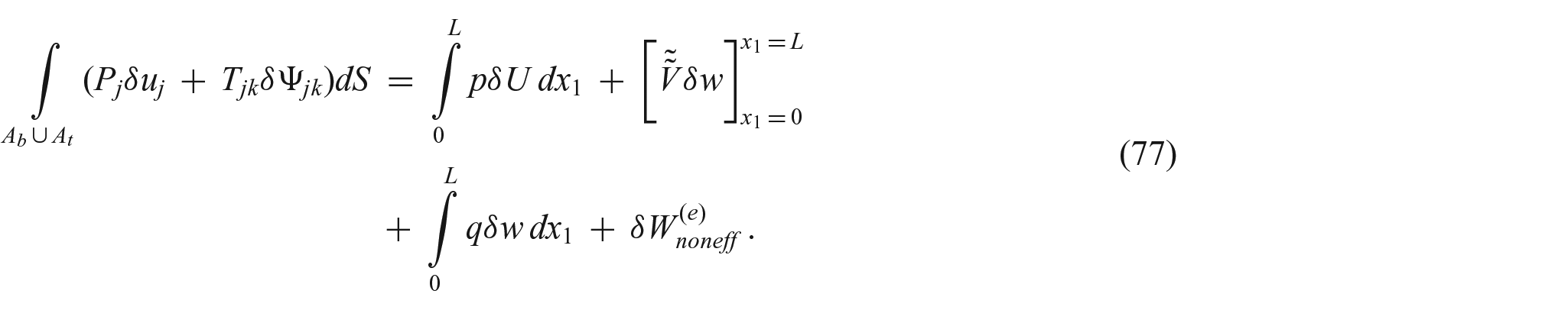
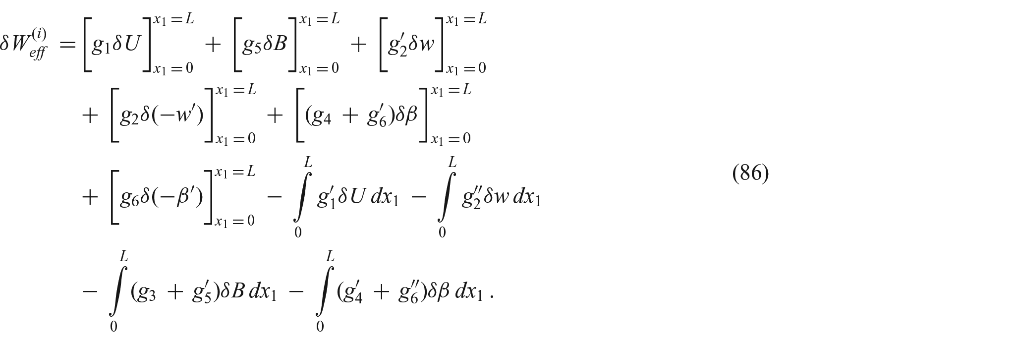
After substitution of equations (77) and (61) into equation (41), keeping in mind definition (43), we can express

and call
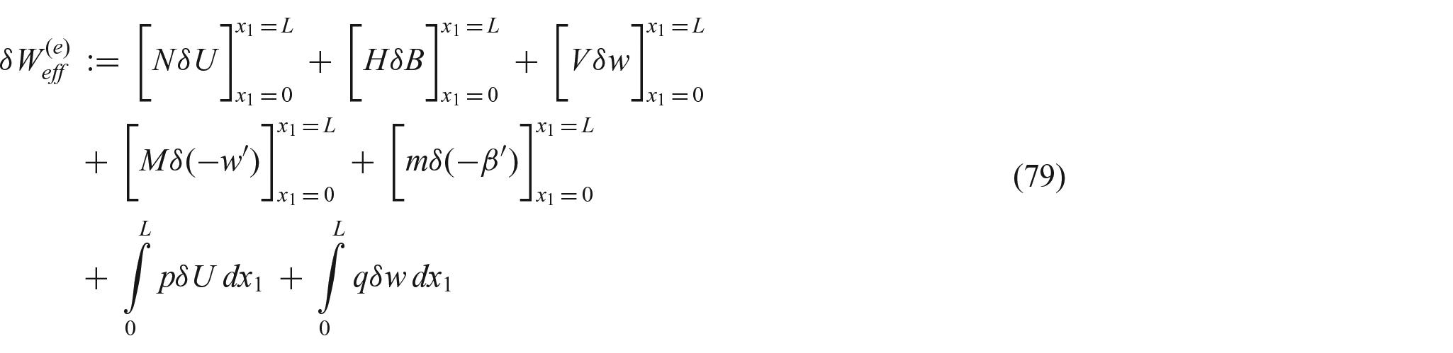
as the effective virtual work of external forces.
4.2.2. Virtual work of internal forces
The virtual work of the internal forces,
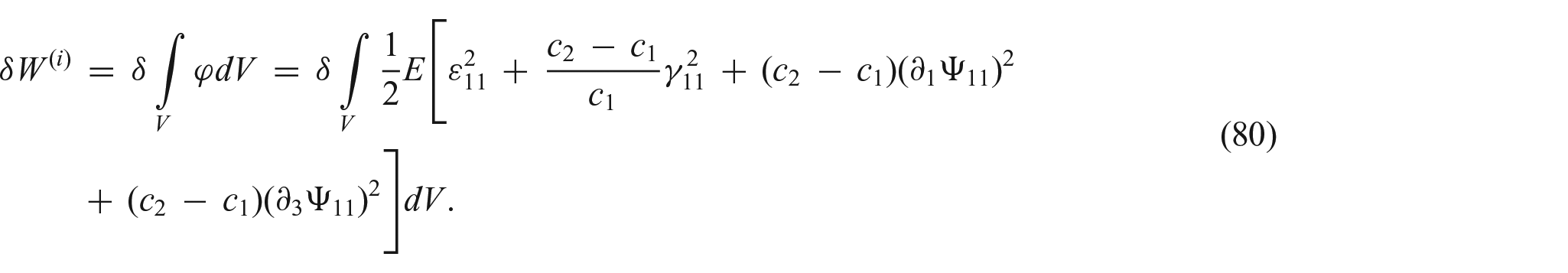
In analogy to equation (78), and recalling from equations (27) and (33) that

where the effective virtual work of the internal forces,

and

For later reference, we use relations (29), (30) and (32) to rewrite

By invoking equation (14)2, we find from equation (82) that
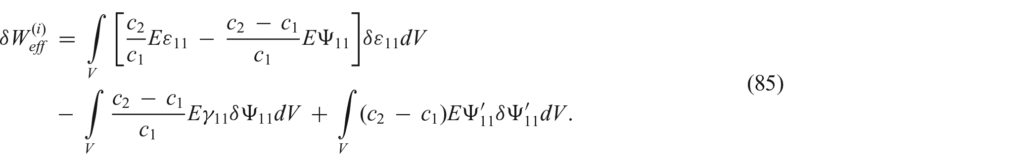
This virtual work can be recast by appealing to equations (26) and (27) for
4.2.3. Virtual work principle, governing equations, boundary conditions
The virtual work principle states for the beam, and for any subbody of it, that

We recognize from equations (83) and (76) that

so that the virtual work principle (87) turns out to be equivalent to the virtual work principle

Bearing in mind equations (79) and (86), we deduce from equation (89) the equations


the relations

and the boundary conditions for section forces


have to be prescribed at
It is not difficult to verify that equations (90), (91), and relations (92) give


which are expressed solely in terms of section forces and resultant forces.
While equations (96) are classical, equations (97) are not. Note also that equations (92)1, (92)2, (92)4, and (92)5 are nothing but the sectional elasticity laws (49)–(52).
We now can summarize the two interpretations of the 3-PG-Model. The first one assumes the material body as particular case of a micromorphic elastic material, so that equations (9) represent non-classical equilibrium equations and
The second interpretation considers equations (9), together with equations (10)–(13), as non-classical constitutive equations. In this case,
4.3. Alternative and equivalent approach
Evidently, the virtual work principle (88), and the governing equations (96), (97), implied by this principle, should also be derivable from the field equations (36)–(40). Indeed, we shall prove in the two following sections that 1) equations (96), (97) might be derived directly from the field equations (36)–(40) and that 2) the virtual work principle (88) might also be derived from the field equations (36)–(40).
4.3.1. Alternative derivation of the governing equations for the section forces
The procedure for deriving equations (96), (97) directly from the field equations (36)–(40), is the same as in engineering mechanics. First we take the integral of equation (36) over

Then, using the definitions (42)1, and (48), equation (98) furnishes equation (96)1.
Next, we integrate equation (37) over

and use definitions (44)1, (47)2, to obtain

In this equation, we set

and by invoking equation (47)1, we arrive at equation (96)2.
In order to derive equation (96)3, we multiply equation (36) by

or
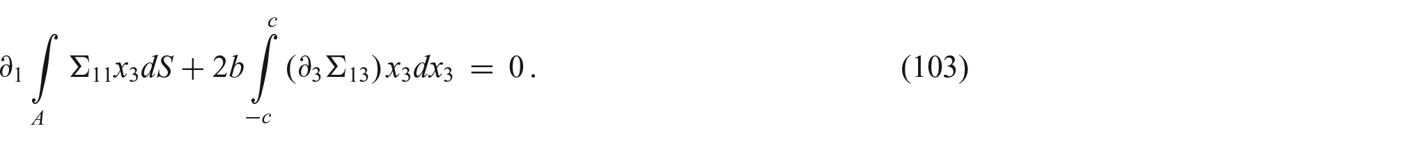
By applying partial integration to the second integral in equation (103),

If we replace the first term with

From this, we obtain equation (96)3 by taking into account the definition of
Before going to establish equations (97) from the field equations, we would like to remark the following. Equations (39), (40) involve only stresses not determinable by constitutive law, and hence these stresses cannot affect the proper governing equations of the beam. Therefore, in order to establish equations (97), we need to elaborate only equation (38). More precisely, take the integral of equation (38) over

and use definitions (45)1, and (46)1, to obtain equation (97)1. Finally, multiply equation (38) by

This equation, together with definitions (45)2 and (46)2 lead to equation (97)2, which completes the derivation of equations (96), (97) directly from the field equations.
4.3.2. Alternative derivation of the virtual work principle
=
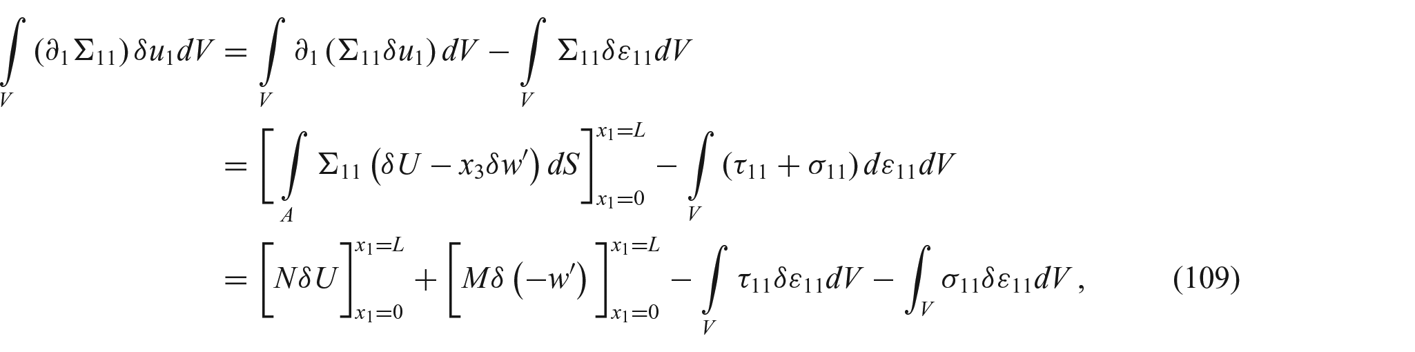
It has been clear in the last section that the relevant field equations for the beam are equations (36)–(38), so we shall now derive the virtual work principle (88) from these equations. We start with the equilibrium equations (36), (37), by forming the scalar product with

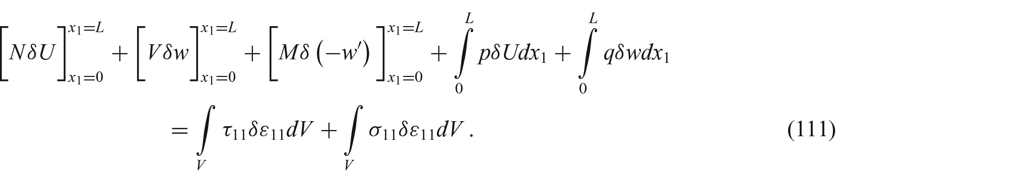
We shall recast this equation by employing equations (25), (26), (31), definitions (42)–(48), as well as partial integration:
After substituting of equations (109), (110) in equation (108), we find that
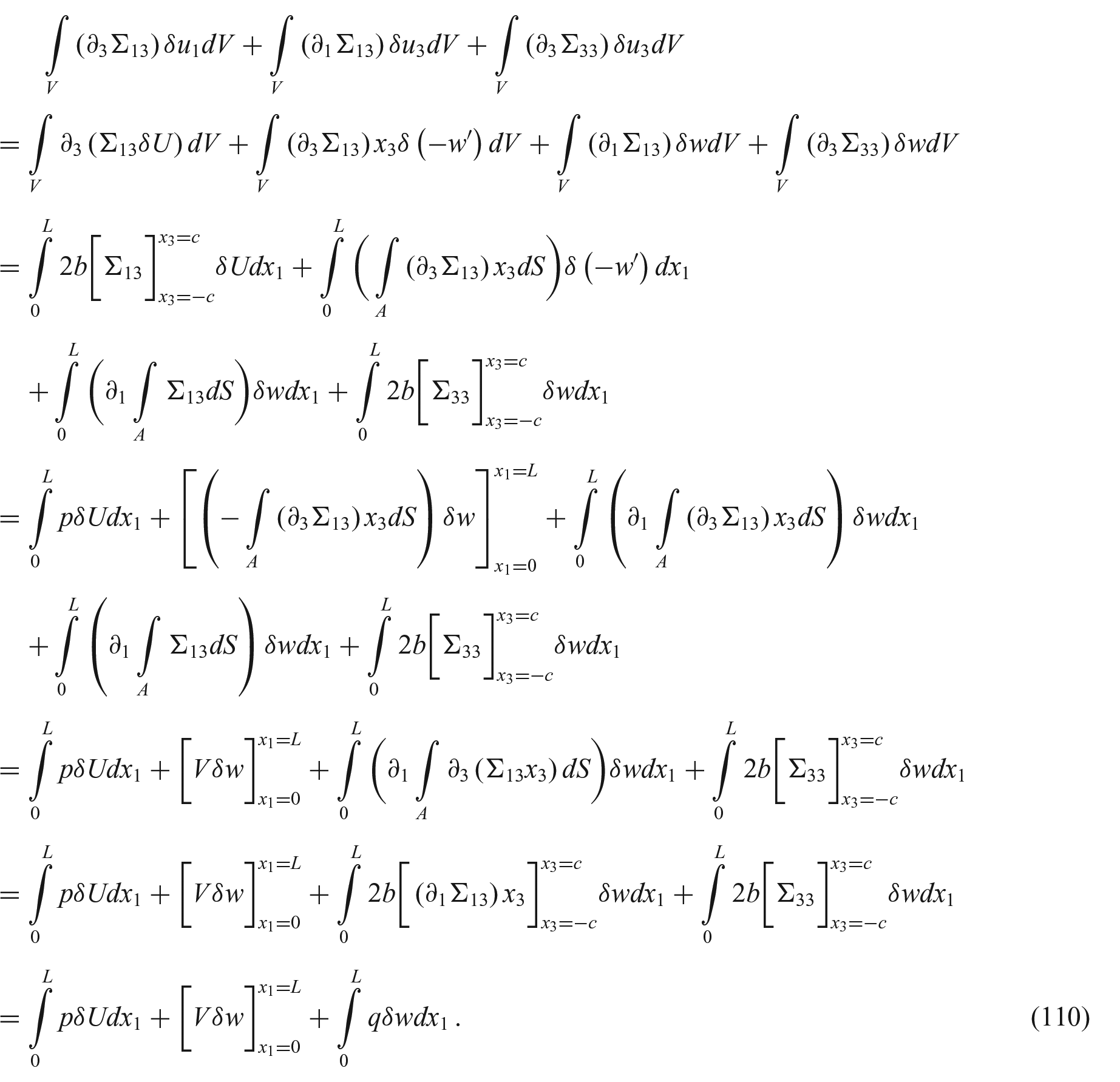
Similarly, multiplication of equation (38) with
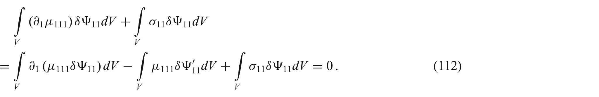
We may use the kinematical relation (27) and the definitions (45) to rewrite the first integral on the right-hand side of equation (112) as
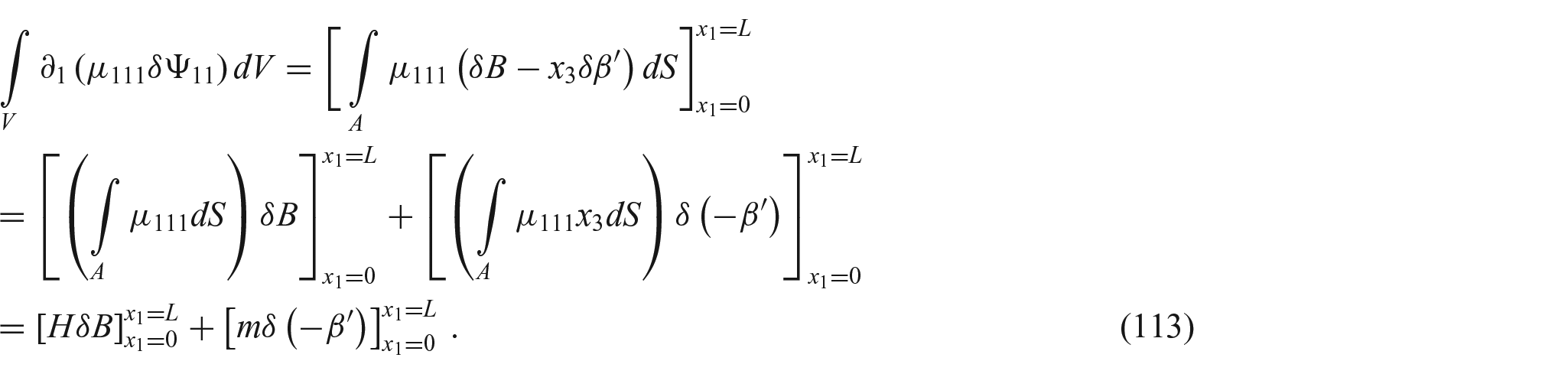
Using this result, we find from equation (112) that

Adding equations (111) and (114), we have
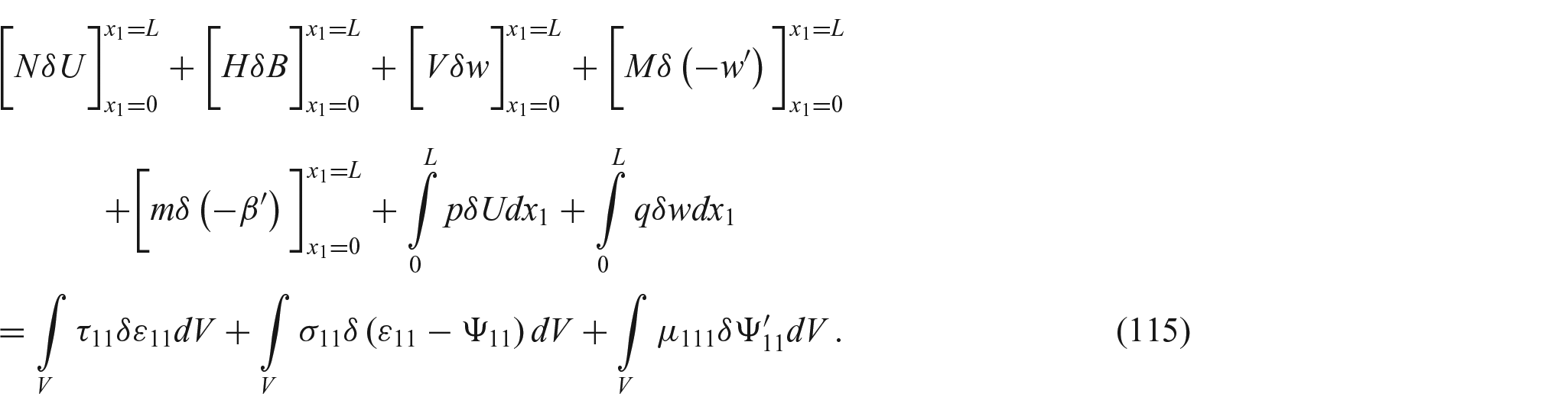
Recalling the kinematical relation (14)2 and the relations (79), (84), we infer from equation (115) that
4.4. Discussion
As stated in the introduction, the Euler–Bernoulli beam theory in common use is based on two fundamental assumptions: 1) The material behavior is isotropic elastic. 2) The plane cross sections of the beam remain plane and perpendicular to the deformed beam-axis and additionally the shape of the cross sections does not change (no deformation).
The two assumptions plainly contradict each other, because according to assumption 2 the material behavior along the cross sections is rigid body like, while along the beam-axis it is elastic. Evidently, assumption 2 presupposes anisotropic material response subject to geometrical constrains, which contradicts assumption 1. The consequence in traditional approaches is that if an isotropic elasticity law holds, than the equilibrium equations cannot be satisfied (inconsistency). Even more, it is not possible to determine uniquely stress components like
There are two possibilities to abolish the inconsistency problem: To modify either assumption 1 or assumption 2. Assumption 2 is very attractive as it leads to a simple deformation geometry. Therefore, assumption 1 has been replaced in Sideris and Tsakmakis [42], Broese et al. [43], and in the present paper, by the assumption of transverse isotropy subject to geometrical constraints. This offered the possibility in the present paper, to derive the one-dimensional virtual work statements by employing both equilibrium equations for stresses and boundary conditions expressed in terms of stresses. This approach made also possible to cancel out the term
4.5. Specific boundary conditions, examples
4.5.1. Vanishing axial load
For the beam in Figure 1, we set (cf. equation (48))

so that, from equations (96)1, (92)1,

Furthermore, we chose for the boundary conditions in equation (93)1

Consequently,

everywhere. Assume now that for some boundary conditions, solutions

On the other hand, from equations (90)2, (51), and (53), we conclude that

We can eliminate

By choosing (cf. equations (93)2, (92)2, (51))

We deduce from the solution of (122), that

Altogether, for the bending problems, we deal with in this section, it remains to solve the governing equations (91),


subject to the boundary conditions (94) and (95),


have to be prescribed at
4.5.2. Distributions of stresses
Suppose that some solutions

By comparison with the response function of

which is the same as in engineering mechanics. Therefore, the distributions of
4.5.3. Cantilever beam subject to uniform transverse load
Under the assumptions made above, we seek solutions

while homogeneous tractions are chosen for the non-classical boundary conditions (129),

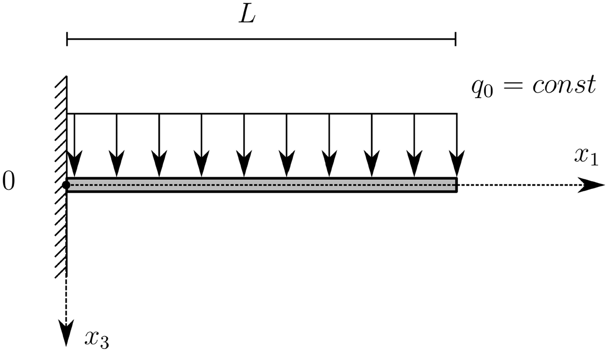
Cantilever beam subject to transverse load
In equations (132) and (133), we can replace the section forces using the sectional constitutive laws (50), (52), and the solution (92)3. An equivalent form of the boundary conditions (132) and (133) is therefore


It is also convenient to refer the governing equations and the concomitant boundary conditions to dimensionless variables. To this end, we introduce the following definitions:


Changing notation in the remainder of the paper, we set

The dimensionless forms of the differential equations (125) and (126) become then


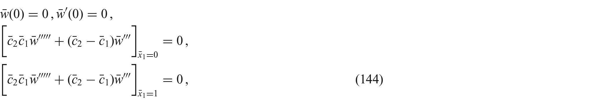
while the boundary conditions (134) and (135) take the forms


Now, a look at the KG- and the 3-PG-Model in equations (2) and (3) could give the impression, that the KG-Model might be viewed as particular case of the 3-PG-Model for
After lengthy, but straightforward manipulations, it can be verified that the system of differential equations (139)–(142) leads to two differential equations, one for

with boundary conditions

and one for

with boundary conditions

There is a constant term in the solution of
The solution of equations (143)–(145) reads

with constants
It is now not difficult to verify, that
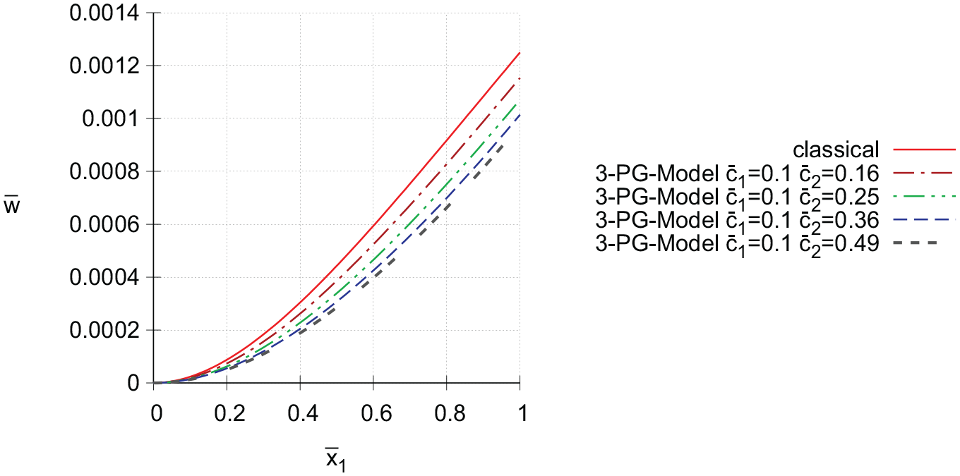
Distributions of
It is remarkable, that the corresponding distributions
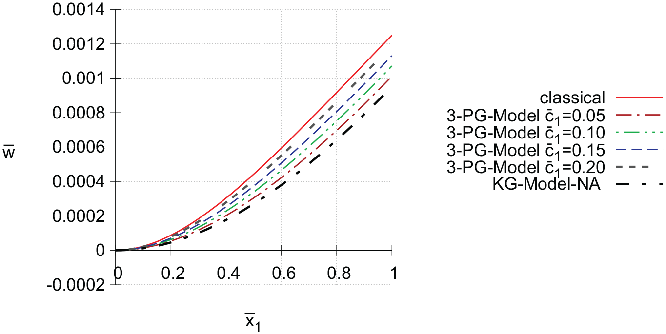
Graph of the curves
Finally, it is perhaps of interest to remark, that for
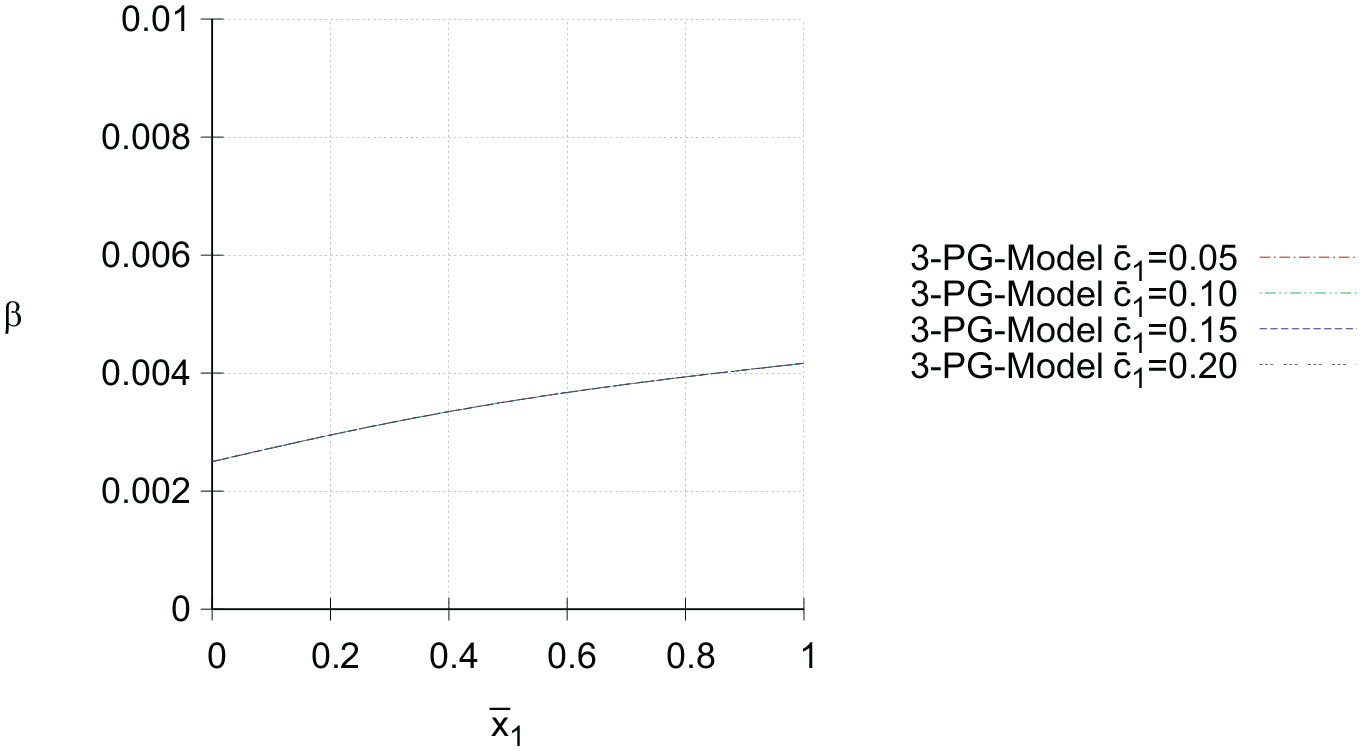
Distributions of
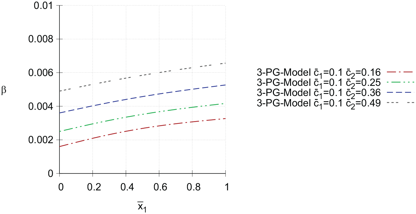
Graph of the curves
5. Conclusion
A consistent Euler–Bernoulli bending theory for gradient elastic beams has been formulated in the paper. The material behavior is described by a gradient elasticity model, called 3-PG-Model, including both the Laplacian of the stress and the Laplacian of the strain. It is the analogon of the Three-Parameter viscoelastic solid. Starting from a standard formulation of the virtual work principle, it is shown that the Euler–Bernoulli geometrical constraints require to consider only an effective part of this principle. Alternatively, this effective work principle can be derived from the field equations of the three-dimensional material body. Moreover, the governing equations of bending might be derived as consequences of the effective virtual work principle, or alternatively directly from the three-dimensional field equations by integration.
Footnotes
Appendix 1
Substitution of equations (26)–(28) into equation (85) yields
By using the relations (55),
with
Appendix 2
Funding
The author(s) disclosed receipt of the following financial support for the research, authorship, and/or publication of this article: The authors acknowledge with thank the Deutsche Forschungsgemeinschaft (DFG) for partial support of this work under Grant TS 29/13-1.