
Abstract
In this study, a new double horizon peridynamics formulation was introduced by utilising two horizons instead of one as in traditional peridynamics. The new approach allows utilisation of large horizon sizes by controlling the size of the inner horizon size. To demonstrate the capability of the current approach, four different numerical cases were examined by considering static and dynamic conditions, different boundary and initial conditions, and different outer and inner horizon size values. For both static and dynamic cases, it was observed that as the inner horizon decreases, peridynamic solutions converge to classical continuum mechanics solutions even by using a larger horizon size value. Therefore, the proposed approach can serve as an alternative approach to improve computational efficiency of peridynamic simulations by obtaining accurate results with larger horizon sizes.
1. Introduction
Although classical continuum mechanics (CCM) has been widely used for the analysis of materials and structures under external loading conditions, equations of CCM are not suitable to represent situations including discontinuities such as cracks since spatial derivatives in CCM equations are not defined along the crack boundaries. Silling [1] introduced peridynamics with the intention to overcome limitations of CCM formulation. By using integro-differential equations without spatial derivatives, peridynamics has become a powerful approach for predicting crack evolution in materials and structures [2]. Rather than using mesh-based or semi-analytical approaches [3], peridynamics formulation is usually numerically implemented by utilising meshless approach. There has been significant progress on peridynamics especially during recent years. Among numerous studies in the field, Vazic et al. [4] demonstrated the superior capability of peridynamics in fracture analysis by investigating the interaction of macro and micro cracks. De Meo et al. [5] predicted pit-to-crack transition process within peridynamic frameworks. Imachi et al. [6] performed dynamic crack arrest analysis by using peridynamics. Ozdemir et al. [7] used peridynamics to investigate functionally graded materials and their dynamic fracture behaviour. Liu et al. [8] analysed fracture of zigzag graphene sheets by creating an ordinary state-based peridynamic model. Huang et al. [9] extended the capability of peridynamics for visco-hyperelastic materials. Diehl et al. [10] presented a review of benchmark experiments for peridynamic models. Zhou and Yao [11] proposed a new concept of smoothed bond-based peridynamics. Prakash and Stewart [12] demonstrated how to use a multi-threaded method to assemble a sparse stiffness matrix for quasi-static problems of peridynamics. Naumenko et al. [13] compared experimental and peridynamic results for damage patterns in float glass plates. Yan et al. [14] used peridynamics to model soil desiccation. Hidayat et al. [15] provided a review about relationships between meshfree methods and peridynamics. Guski et al. [16] utilised peridynamics to investigate plasma sprayed coatings for Solid Oxide Fuel Cell (SOFC) sealing applications. Kefal et al. [17] demonstrated how to use peridynamics for topology optimisation of cracked structures. There have also been many studies presenting peridynamic formulations for beams and plates to model isotropic materials [18–22], functionally graded materials [23–28], and composite materials [29,30]. Peridynamics has also been extended to model other physical fields. Mikata [31] presented peridynamic formulations for fluid mechanics and acoustics. Diyaroglu et al. [32] introduced a peridynamic wetness approach to be utilised for the analysis of moisture concentration in electronic packages. Martowicz et al. [33] created a thermomechanical model to investigate phase transformation in shape memory alloys.
An important aspect of peridynamics is its length scale parameter, horizon, which does not exist in CCM formulation. Dorduncu and Madenci [34] presented a finite element implementation of ordinary state-based peridynamics having variable horizon. Madenci et al. [35] developed a weak form of bond-associated non-ordinary state-based peridynamics formulation for uniform or non-uniform discretization without experiencing zero-energy mode problem. A comprehensive investigation on how to choose horizon size in bond-based peridynamics and state-based peridynamics is given in Bobaru and Hu [36] and Wang et al. [37], respectively. In this study, a new peridynamic formulation, double horizon peridynamics (DH PD), is proposed, which utilises two horizons for each material point instead of one horizon as in traditional peridynamics formulation. Since simulation-based traditional peridynamics can take significant computational time, for some cases, if a large horizon size and/or refined discretization are utilised, this new formulation can allow improvement of numerical accuracy in peridynamic simulations with less computational time. This formulation is different than “DH PD” formulation, which uses two different horizons for two interacting material points [38–41]. The details of the “DH PD” formulation is given in Section 2. How to treat boundary conditions is explained in Section 3. Analytical solutions for various different boundary conditions under static or dynamic conditions are given in Sections 4 and 5. Some numerical results are presented in Section 6, and conclusions of the study are given in Section 7.
2. DH PD formulation
2.1. Traditional peridynamics
The equation of motion (EoM) for a one-dimensional (1D) rod in CCM can be written as,

peridynamics (PD) EoM for 1D bar can be obtained by converting the local term in equation (1) into nonlocal form by utilising Taylor expansion. Performing Taylor expansion with respect to displacement function

Considering
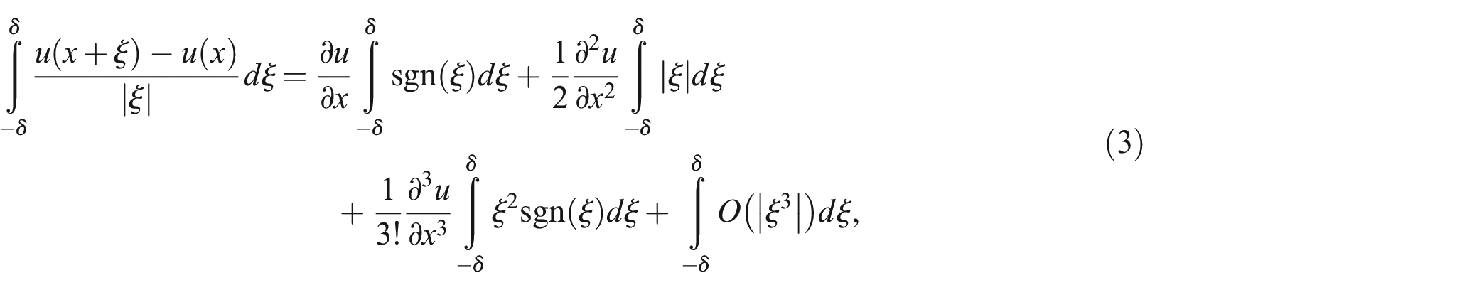
which gives,
Substituting equation (4) into equation (1) yields,
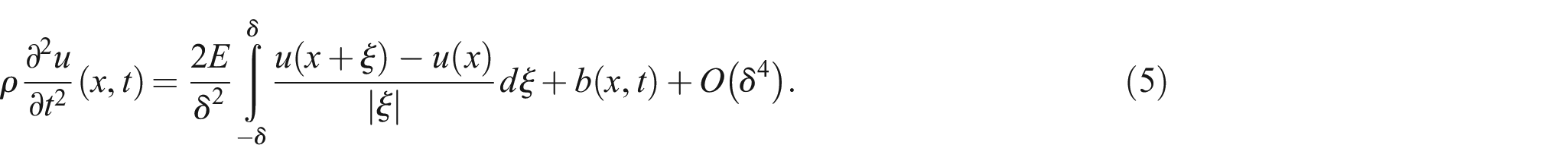
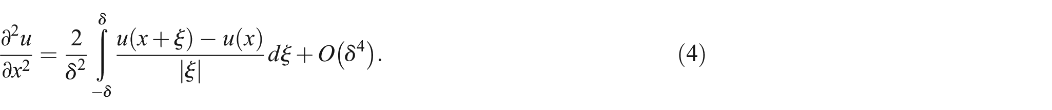
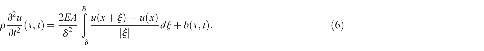
It reduces to the classic PD EoM if we eliminate the residual term in the above equation such that,
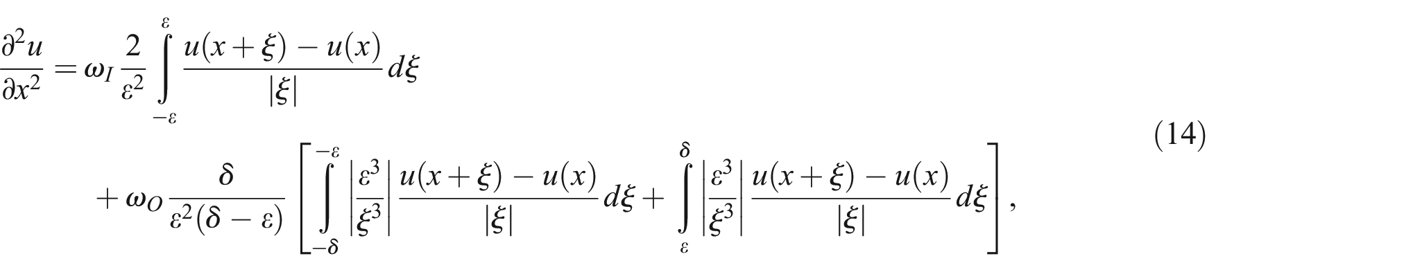
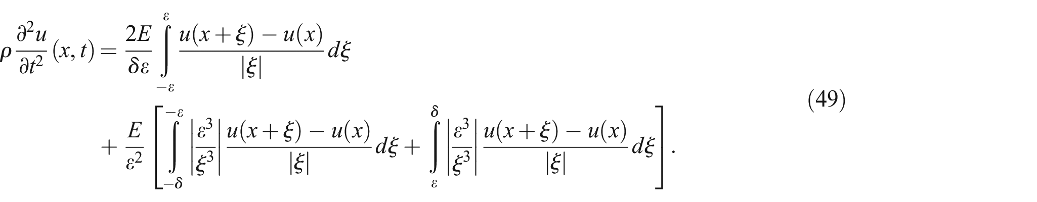
2.2. DH PD
One can observe that the classical PD EoM, equation (6) identically converges to that of CCM, equation (1) if and only if when the horizon size,
Consider a small inner horizon inside the original horizon as shown in Figure 1.
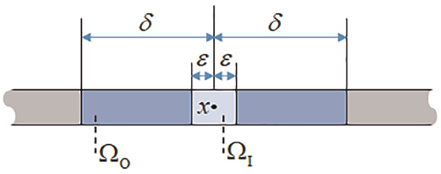
The inner horizon
First, let us consider the integration over the inner horizon
Note that the inner horizon size
Next, let us consider the integration over the outer horizon

Note that when

In order to reduce the residual to be consistent with that of the inner horizon, multiplying equation (8) by

Now considering
Ignoring residual gives,
Introducing two weight functions

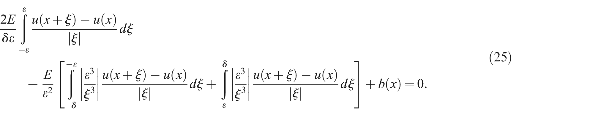
and combining equation (7) with equation (12) gives,
in which the weight functions can be chosen by considering each horizon size in proportion to the total horizon size as,

Coupling equation (15) with equation (14) and substituting into equation (1) yields the refined PD EoM for 1D bar as,
Note that when the inner horizon size equals to the outer horizon size,
3. Boundary conditions
From a PD point of view, except for the damage situation, each material point must be completely embedded in its PD influence domain. Moreover, for those material points adjacent to the boundary, whose domain is incomplete, it is necessary to introduce fictitious regions outside the boundary such that the completeness of PD EoM is ensured. The width of fictitious region can be chosen as equal to the horizon size
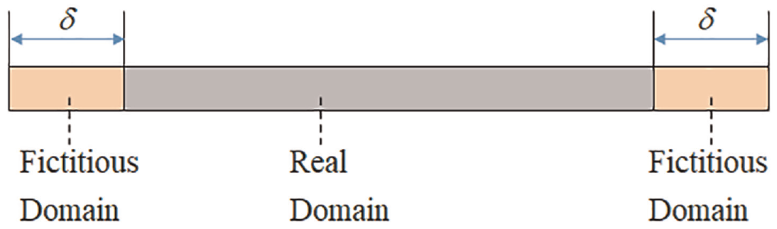
Real and fictitious domains.
3.1. Fixed boundary conditions
Recall the EoM in classical elasticity:

Suppose the body is constrained at

One can obtain by performing central difference for equation (18) that,

where

Here, the material point
3.2. Neumann boundary conditions
Suppose the body is subjected to a concentrated load of

Again, performing central difference with respect to

After performing some algebra and rearranging the central difference notation according to PD convention, one can obtain that,

Note that,

and equation (24) is called the free boundary condition relationship in the PD framework.
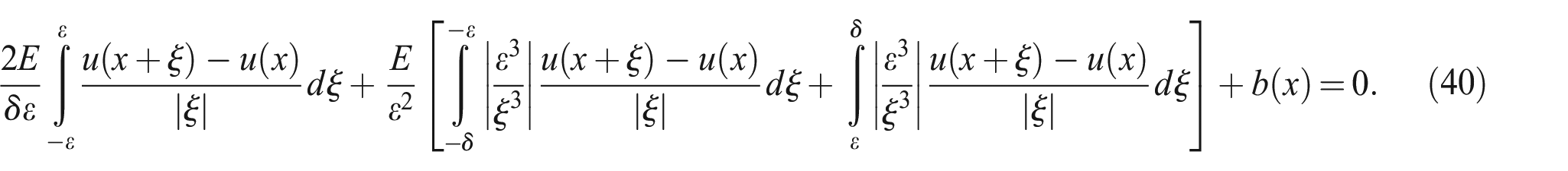
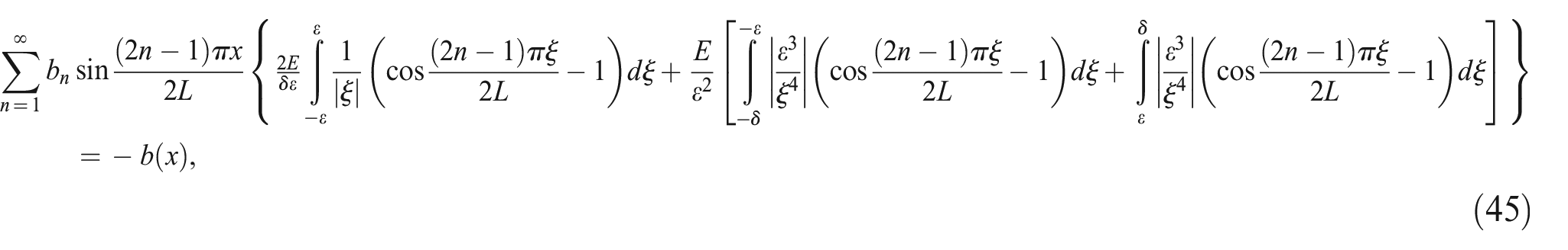
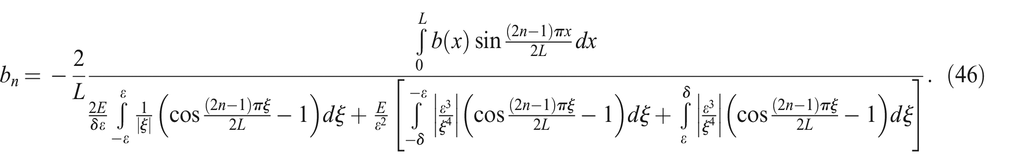
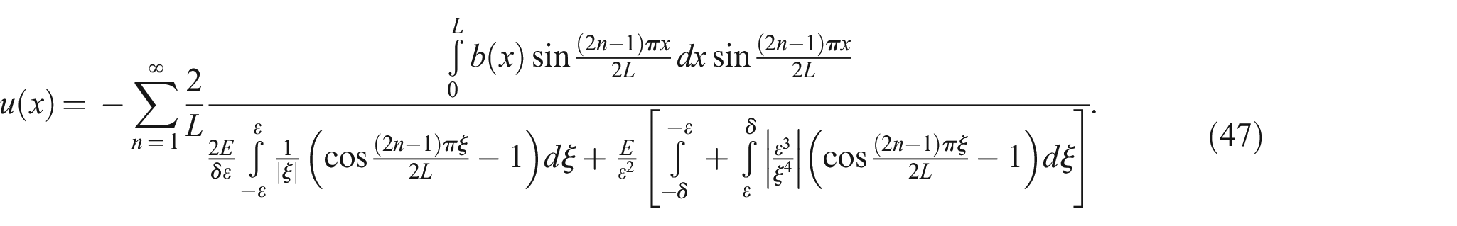
4. Analytic solutions for static problems
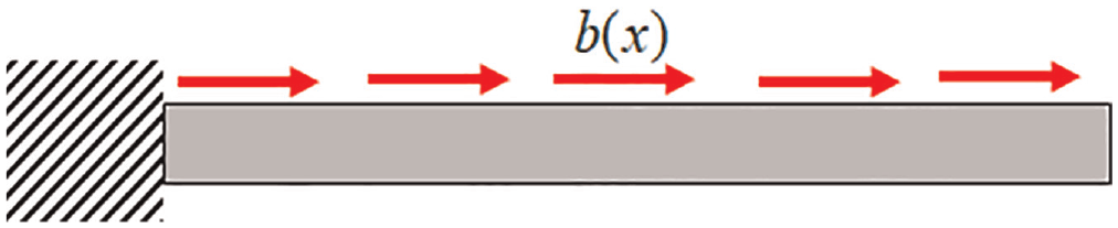
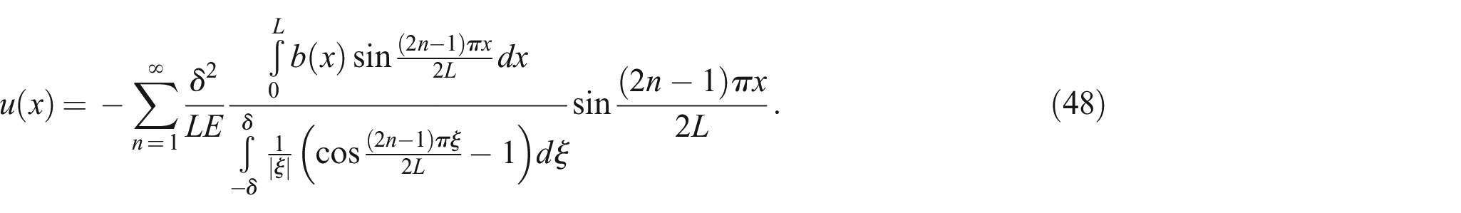
4.1. Fixed–fixed rod
Consider a rod subjected to fixed–fixed boundary condition and arbitrary distributed loading as shown in Figure 3.
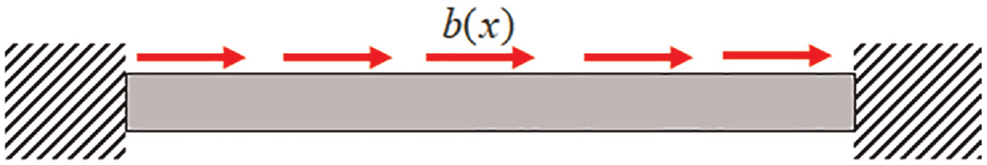
Rod subjected to fixed–fixed boundary condition and arbitrary distributed loading.
The length of the bar is denoted as

According to the completeness characteristic of a trigonometric system, it is reasonable to assume that the displacement function accommodates in the vector space spanned by trigonometric functions, i.e.,

which can be expressed as a linear combination in terms of the bases as follows:

Substituting equation (28) into equation (26a) yields,

Without considering rigid body motion, one can obtain that,

Substituting equation (30) into equation (26b) yields,

which gives,

Plugging equation (32) back into equation (30) implies,

One can obtain that,
Similarly,
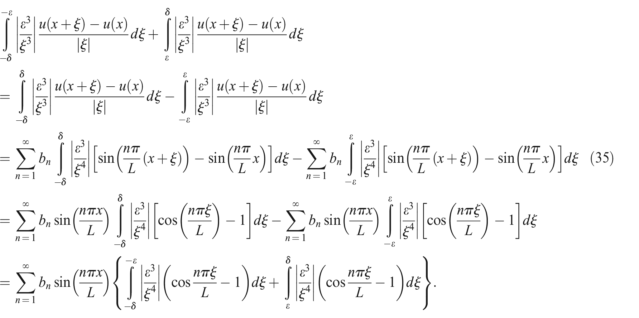
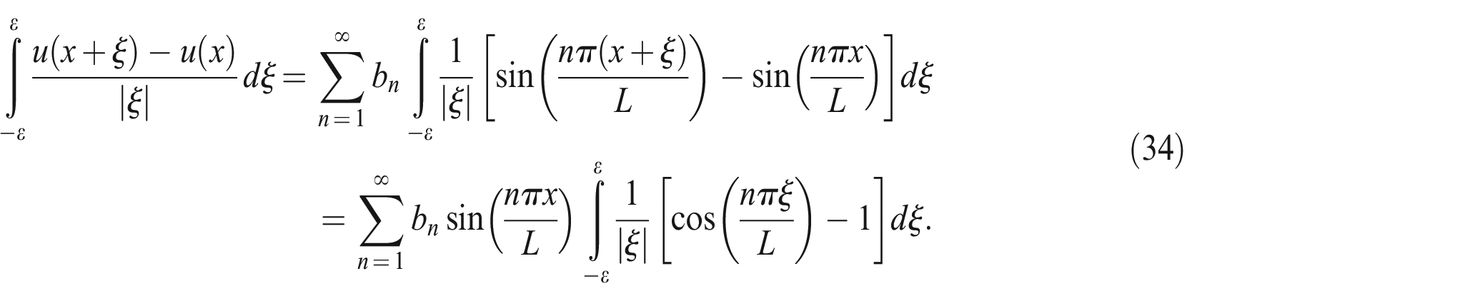
Substituting equations (34) and (35) into equation (25) yields,
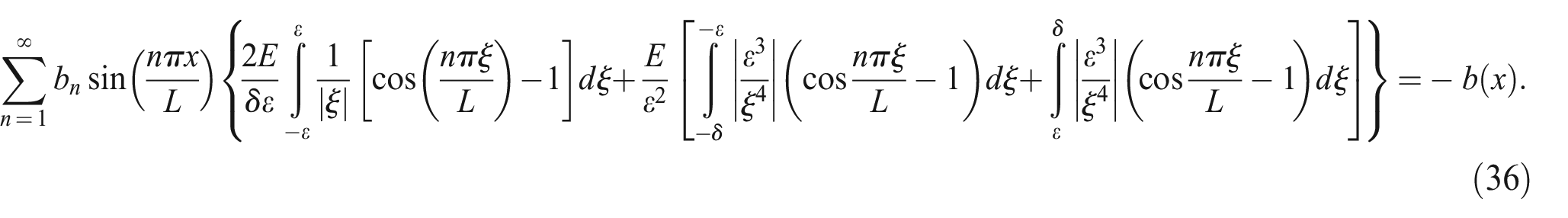
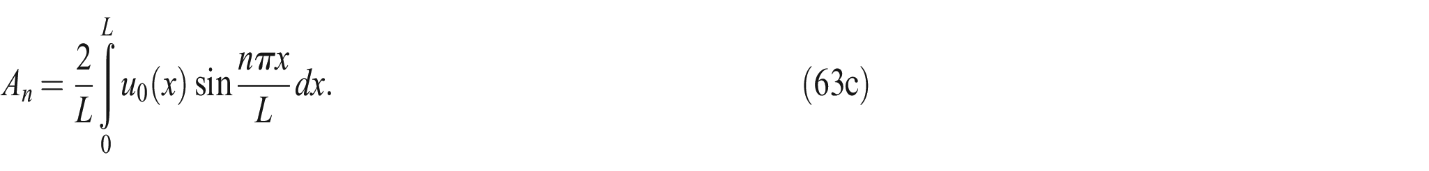
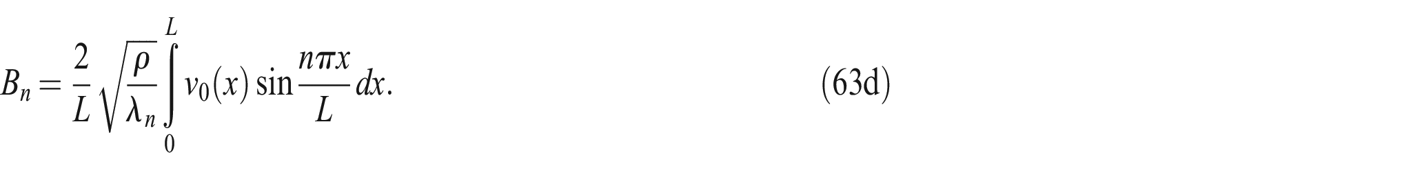
According to the orthogonal property of trigonometric functions, the coefficients can be determined as,
Hence, the analytical PD solution is,
Note that when
4.2. Fixed–free rod
Consider a rod subjected to fixed–free boundary condition and arbitrary distributed loading as shown in Figure 4.
Rod subjected to fixed–free boundary condition and arbitrary distributed loading.
The PD EoM and BCs for this case can be expressed as,

Again, suppose the displacement function belongs to the vector space spanned by bases of trigonometric functions and hence can be expressed as,

Using equations (41a, b), one can obtain,

and,

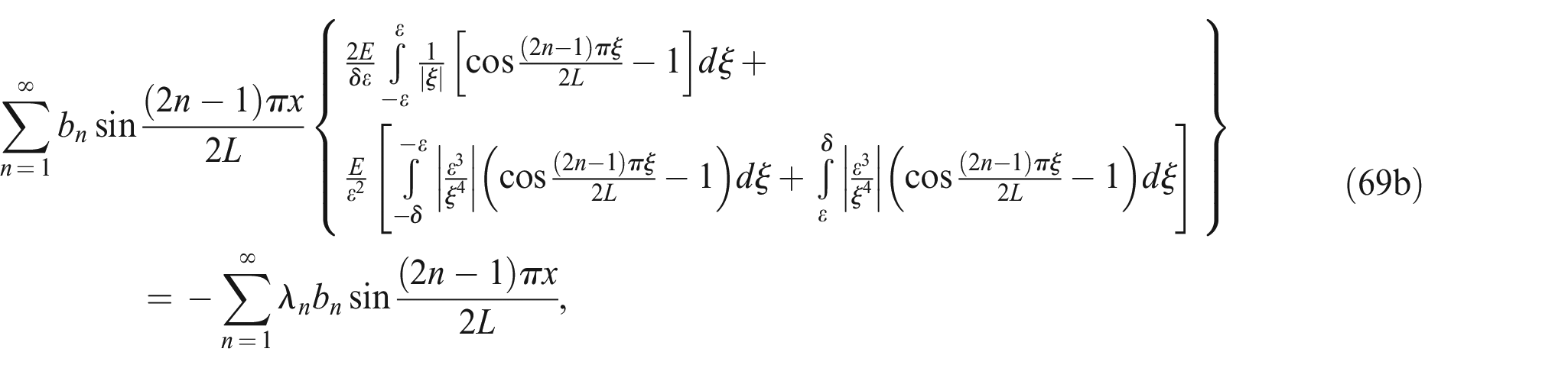
Plugging equation (44) back into equation (40) and performing algebraic simplifications results in,
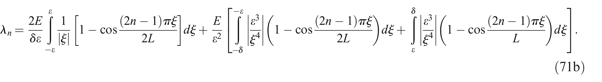
where the coefficients can be determined as,
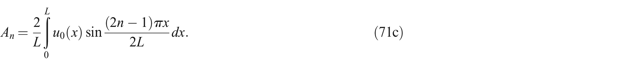
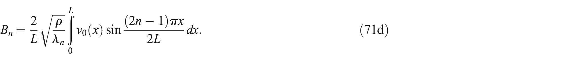
Substituting equation (46) into equation (44) yields the PD analytical solution as,
In particular, when
5. Analytical solutions for free vibration condition
5.1. Fixed–fixed rod
Let the PD EoM, BCs, and Initial Condition (IC)s to be expressed for the fixed–fixed rod as,


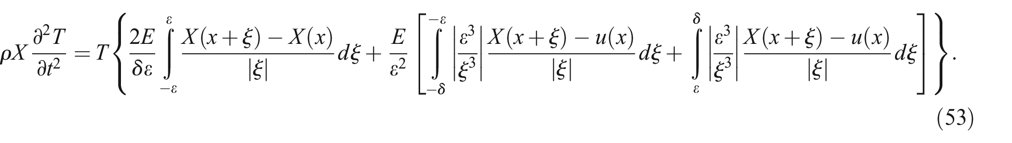
By using separation of variables approach, the displacement function can be decomposed as,

Hence, equation (49) can be rewritten as,
Isolating variables yields,
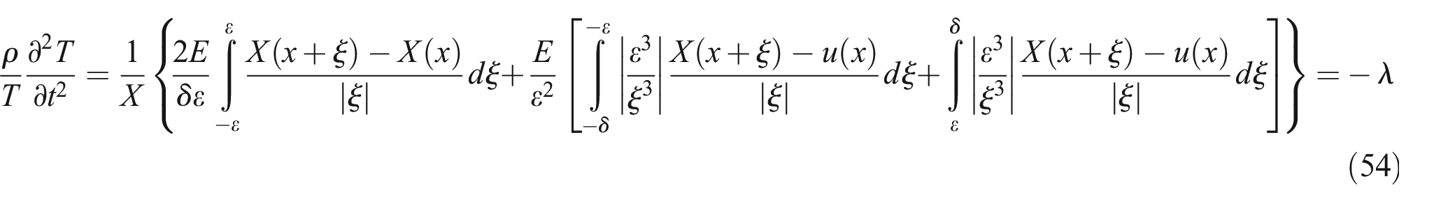
which gives,
and,

By comparing equation (55a) with equation (25), we can consider

and,
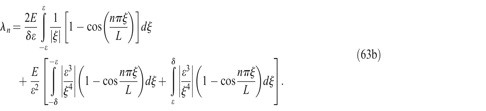
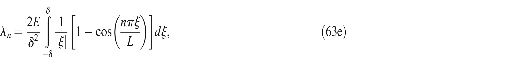
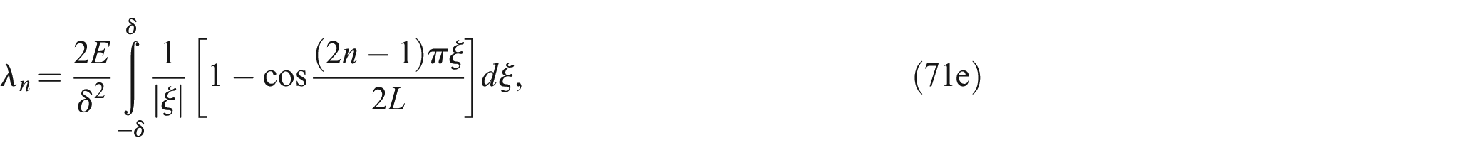
which results in the PD “eigenvalues” as,
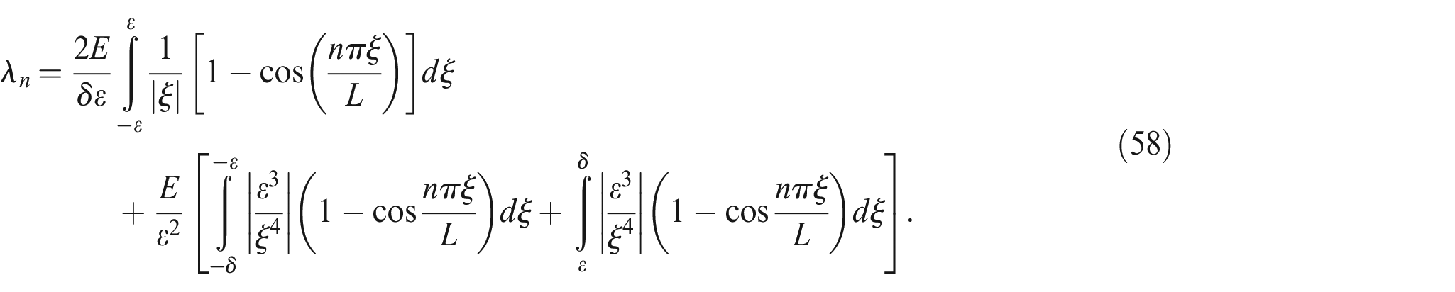
The general solution to equation (55b) can be expressed as,

Substituting equations (59) and (56) into equation (52) and rearranging the coefficient notations yields the general PD solution as,

Differentiating equation (60) with respect to time yields,
Applying the ICs gives,
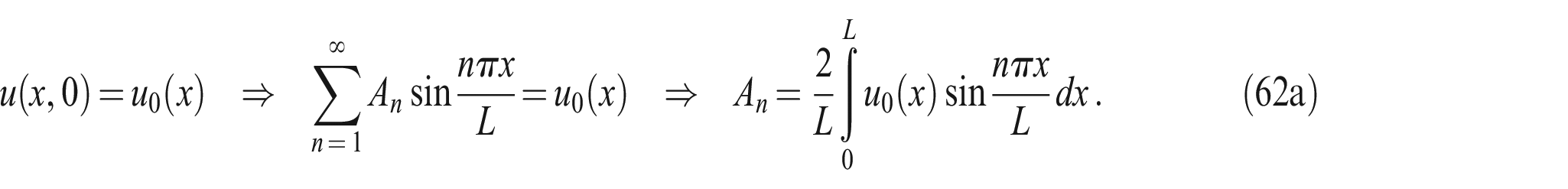
As a summary, the PD analytical solution for free vibration of fixed–fixed rods can be summarised as,
In particular, when
which is valid for traditional PD models.
5.2. Fixed–free rod
Let the PD EoM, BCs, and ICs for the fixed–free rod be expressed as,


By using separation of variables approach, i.e.,

two characteristic functions can be obtained by substituting equation (67) into equation (64) as,
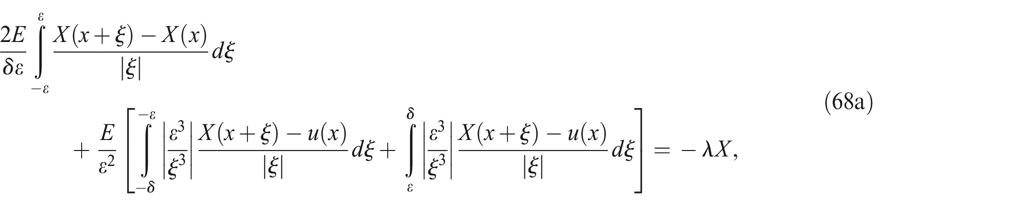
and,

By comparing equation (68a) with equation (40), we can consider

and,
which results in the PD “eigenvalues” as,
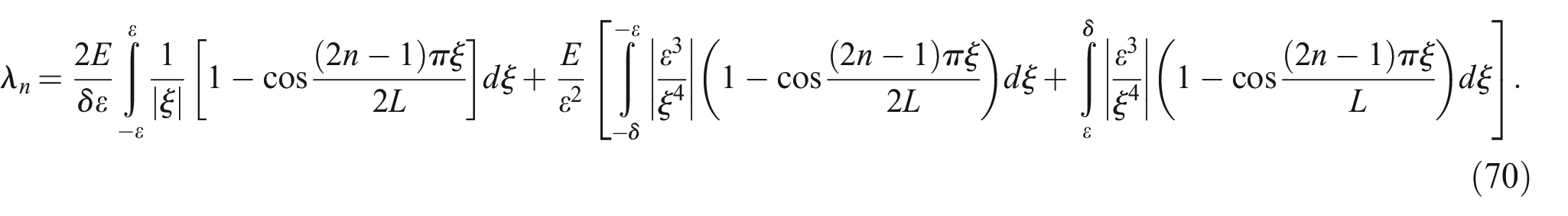
Similar to the derivations of the previous case, the refined PD analytical solution can be obtained as,

In particular, when
which is valid for the traditional PD model.
6. Numerical results
6.1. Fixed–fixed rod under static conditions
In the first case, a 1D rod with a length of L = 1 m is subjected to a body load of b(x) = 1000(1 –x)10 N/m3 under static conditions. Both edges of the rod are fixed (fixed–fixed). Elastic modulus of the rod is specified as E = 200 GPa.
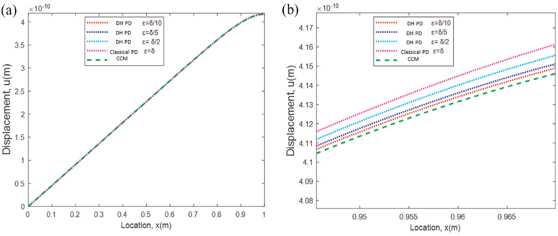
Variation of the displacement field along the rod by changing inner horizon size, ε = δ, δ/2, δ/5, δ/10, for a horizon size value of δ = 0.1 m are given in Figure 5. As shown in this figure, as the size of the inner horizon decreases, DH PD solution converges to the CCM solution.
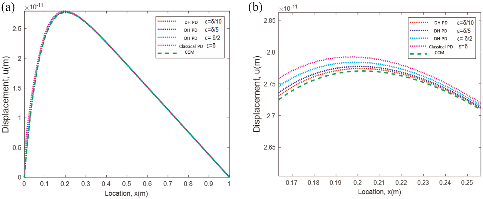
(a) Variation of the displacement field along the rod by changing inner horizon size, ε, for a horizon value of δ = 0.1 m and(b) Zoomed view.
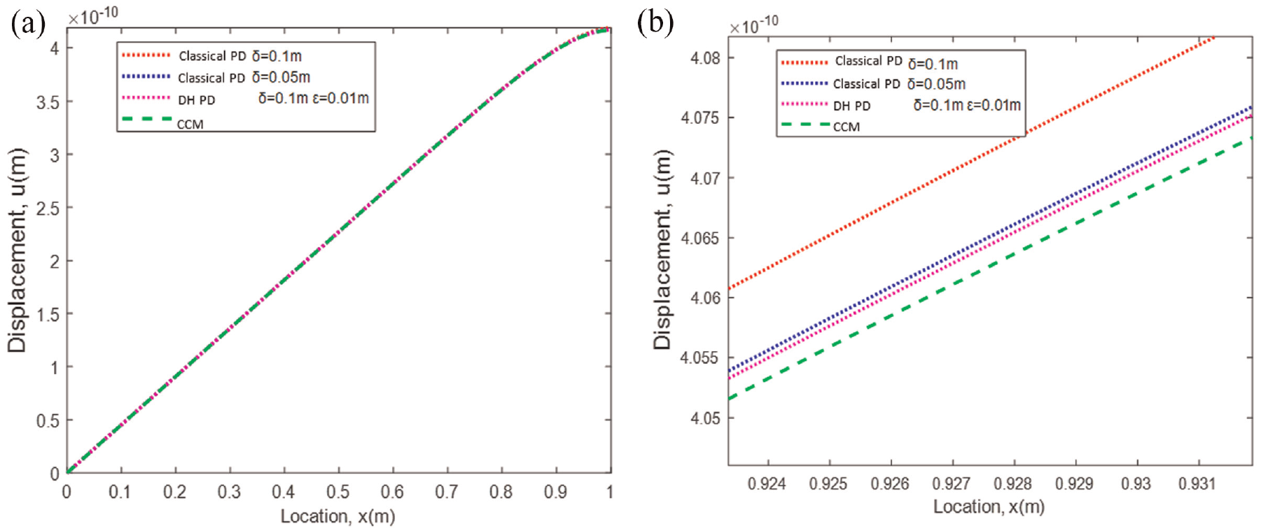
In Figure 6, two different scenarios are compared. First, as the horizon size decreases from δ = 0.1 m to δ = 0.05 m, peridynamic solution converges to the CCM solution as expected. On the contrary, even if a larger horizon size is used, i.e., δ = 0.1 m, the new DH PD approach provides closer results to CCM solution for an internal horizon size of ε = 0.01 m.
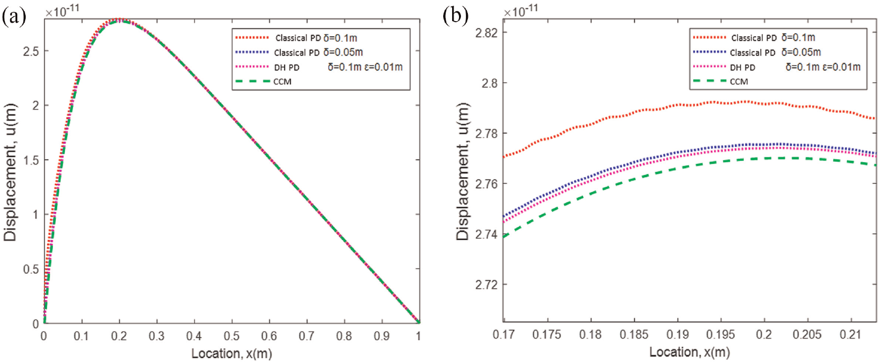
(a) Variation of the displacement field along the rod by changing the horizon size and using a traditional or double horizon approach and (b) Zoomed view.
6.2. Fixed–free rod under static conditions
In the second case, the same properties are considered as in the first case except the right edge is left as free condition whereas the left edge is fixed under static conditions. First, the effect of the internal horizon size is investigated by changing the inner horizon size as ε = δ, δ/2, δ/5, δ/10, for a horizon size value of δ = 0.1 m. As shown in Figure 7, as the inner horizon size decreases, DH PD results converge to the CCM solution based on the variation of displacements along the rod.
(a) Variation of the displacement field along the rod by changing inner horizon size, ε, for a horizon value of δ = 0.1 m and (b) Zoomed view.
Next, two different horizon size values are considered, δ = 0.1 m, 0.05 m, by using traditional peridynamics and as expected, for the smaller horizon size value, peridynamic results are closer to CCM results (see Figure 8). On the contrary, if DH PD formulation is utilised, better agreement can be obtained even for a larger horizon size δ = 0.1 m by considering the inner horizon size as ε = 0.01 m.
(a) Variation of the displacement field along the rod by changing the horizon size and using a traditional or double horizon approach and (b) Zoomed view.
6.3. Fixed–fixed rod under free vibration conditions
In the third case, the capability of the DH PD formulation under the dynamic free vibration conditions is investigated. The length of the rod is the same as the two previous cases. The horizon size is specified as δ = 0.1 m. Elastic modulus and density are given as E = 200 GPa and ρ = 7850 kg/m3. Initial conditions are imposed as,


As shown in Figure 9, the variation of the displacement at the centre of the rod (x = 0.5 m) as the time progresses is obtained by changing the internal horizon value as ε = δ, δ/5, δ/10, δ/100. Similar to the static cases, as the internal horizon size decreases, DH PD results capture the CCM results very well for the same outer horizon size value which demonstrates the capability of the double horizon approach.
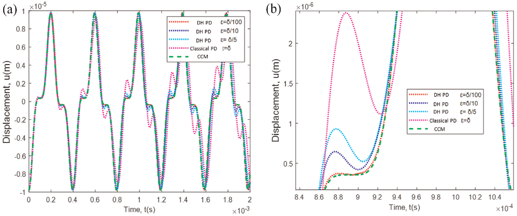
(a) Variation of the displacement field at the centre of the rod (x = 0.5 m) by changing inner horizon size, ε, for a horizon value of δ = 0.1 m and (b) Zoomed view.
6.4. Fixed–free rod under free vibration conditions
In the final numerical case, the same properties are considered as in the previous case except by assigning free condition for the right edge and fixed condition for the left edge under free vibration conditions and imposing the initial conditions as,


As in the previous case, four different internal horizon values are considered as ε = δ, δ/5, δ/10, δ/100, and the variation of the displacement at the centre of the rod (x = 0.5 m) is obtained as the time progresses as shown in Figure 10. Similar to the previous case, DH PD results match very well with the CCM results as the internal horizon size decreases.
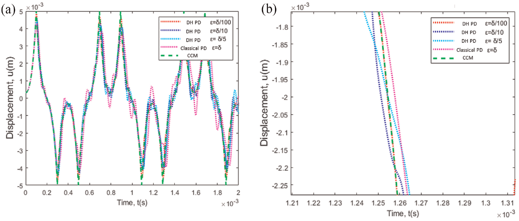
(a) Variation of the displacement field at the centre of the rod (x = 0.5 m) by changing inner horizon size, ε, for a horizon value of δ = 0.1 m and (b) Zoomed view.
7. Conclusion
In this study, a new DH PD formulation was introduced by utilising two horizons instead of one as in traditional peridynamics. To demonstrate the capability of the current approach, four different numerical cases were examined by different boundary (fixed–fixed and fixed–free) and initial conditions under static and dynamic conditions for different outer and inner horizon size values. For both static and dynamic cases, it was observed that as the inner horizon decreases, peridynamic solutions converge to CCM solutions even by using a larger horizon size value. Therefore, the proposed approach can serve as an alternative approach to improve computational efficiency of peridynamic simulations by obtaining accurate results with larger horizon sizes. Potential future directions can be extending the current formulation to two-dimensional and three-dimensional models, and problems including fracture.