Clarification of Faber series and related applications to complex variable methods in two-dimensional elasticity

Abstract

Faber series are used extensively in the application of complex variable methods to two-dimensional elasticity theory, for example, in the mechanical analysis of composite materials where Faber series representations of complex potentials lead to convenient expressions for the corresponding displacement and stress distributions. In many cases, the use of the Faber series is combined with conformal mapping techniques which “transfer” a boundary value problem defined in the elastic body (physical plane) to a simpler problem posed in an imaginary plane characterized by the conformal mapping. In several instances in the literature, however, little attention has been paid to the domain of definition of the Faber series in the imaginary plane leading often to misunderstandings and erroneous conclusions regarding the concept and feasibility of the use of the Faber series. In this paper, we present a thorough and rigorous examination of the representation of the Faber series in both the physical (occupied by the material) and imaginary (defined by the conformal mapping) plane. In addition, we show that replacing a truncated Faber series by a truncated Taylor series does not induce any additional errors in the numerical analysis of the corresponding boundary value problem. We anticipate that the discussion in this paper will help clarify any existing misinterpretations regarding the application of the Faber series and help further extend their use to a range of problems in composite mechanics.

1. Introduction

The use of Faber series continues to attract considerable attention in the literature, particularly in the area dealing with composite materials whose phases include arbitrarily shaped elastic inhomogeneities (see, for example, studies [1–6]). Much of the enthusiasm for the use of the Faber series can be attributed to the fact that they allow for simple representation of complex potentials which, in turn, lead to convenient expressions for the corresponding displacement and stress distributions in the material. In many cases, the use of the Faber series is combined with conformal mapping techniques which “transfer” a boundary value problem defined in the elastic body (physical plane) to a simpler problem posed in an imaginary plane characterized by the conformal mapping. In such cases, to facilitate computations, many authors choose to represent the Faber series in the imaginary plane as opposed to the (real) physical plane, but in doing so fail to provide/clarify the corresponding domain of definition of the Faber series in the imaginary plane. This has often led to confusion and misunderstanding among engineering scientists working in this area. For example, Chen [7] remarks that in the paper by Luo and Gao [3], the Faber series representation for the complex potential of the inhomogeneity in the imaginary plane is invalid since the conformal mapping is valid only for the physical region occupied by the matrix and not that occupied by the inhomogeneity. Luo and Gao [8] subsequently responded to the comments made by Chen, but in doing so introduced only simple definitions of Faber polynomials and Faber series which, in the present authors’ opinion, do not adequately answer the concerns detailed by Chen [7]. In this paper, we present a detailed clarification of the properties of Faber polynomials and Faber series in both their original (physical) plane of definition and in the imaginary plane resulting from the use of conformal mapping. In addition, we examine the relation between Faber and Taylor series and their use in numerical computations.

The paper is organized as follows. We review the definition of Faber polynomials and Faber series in section 2. In section 3, we present the original form of Faber polynomials (already available in the literature but often neglected by researchers in applied mechanics) and clarify their corresponding representation in the imaginary plane defined via a conformal mapping. The relationship between Faber series and Taylor series is discussed in section 4. Finally, our main results are summarized in section 5.

2. Faber polynomials and Faber series: concepts

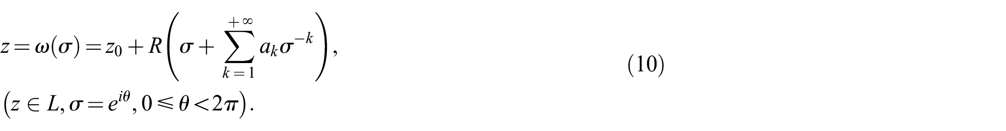
The fundamental concepts behind Faber polynomials and Faber series as well as a comprehensive discussion of their defining properties are given in Curtiss [9]. For completeness, we review the most relevant (for our purposes) properties here and refer the reader in Curtiss [9] for further information. In the infinite Cartesian x₁−x₂ plane or complex z-plane (z = x₁ + ix₂ in which i denotes the imaginary unit), we consider a simply connected finite (open) region S₁ (bounded by an arbitrary smooth closed simple curve L) and the infinite region S₀ exterior to S₁ (see Figure 1). We can always guarantee the existence of a conformal mapping that transforms S₀ in the (physical) complex z-plane to the exterior of the unit circle in the (imaginary) complex ξ-plane. In particular, this mapping can be described in terms of an infinite series as follows [10]:

$$z=\omega \left(\xi \right)=z_0+R(\xi +\sum _{k=1}^{+\infty }{a}_k{\xi }^{-k}),\left|\xi \right|\ge 1,$$

(1)

where z₀ is a specific point inside S₁ which depends on the overall position of S₁ in the z-plane, while the constants R and a_k (k = 1,2,3,…) are determined by the size and shape of S₁ in the z-plane. In particular, equation (1) maps the entire curve L in the z-plane to the entire unit circle in the ξ-plane. The Faber polynomials P_j(z) (j = 0,1,2,…) defined in S₁ are introduced via the following Laurent series expansion of the function $\xi \omega \prime (\xi )/[\omega (\xi )-z]$ holomorphic outside the unit circle in the ξ-plane:

$$\frac{\xi \omega \prime \left(\xi \right)}{\omega \left(\xi \right)-z}=\sum _{j=0}^{+\infty }{P}_j\left(z\right){\xi }^{-j},(\left|\xi \right|\ge 1,z\in S_1),$$

(2)

where, clearly, P₀(z) = 1. In particular, the boundary values P_j(t) ( $t\in L,j=0,1,2,...$ ) on the curve L are defined by the limit of P_j(z) (j = 0,1,2,…) as z tends towards $t\in L$ . Using the Faber polynomials P_j(z) (j = 0,1,2,…), we can find the Faber series expansion of an arbitrary holomorphic function $\phi (z)$ in S₁ whose boundary value is denoted by $\phi (t)$ ( $t\in L$ ). In fact, it follows from Cauchy’s integral formula that

$$\phi \left(z\right)=\frac{1}{2\pi i}\underset{L}{\oint }\frac{\phi \left(t\right)}{t-z}\mathrm{dt},z\in S_1,$$

(3)

which, from equations (1) and (2), becomes

$$\phi \left(z\right)=\sum _{j=0}^{+\infty }{b}_j{P}_j\left(z\right),z\in S_1,$$

(4)

with

$$b_j=\frac{1}{2\pi i}\underset{\left|\sigma \right|=1}{\oint }\phi \left(\omega \left(\sigma \right)\right){\sigma }^{-j-1}d\sigma .$$

(5)

Here, equation (4) gives the Faber series of $\phi (z)$ whose coefficients are defined by equation (5).

Figure 1.

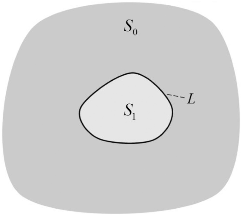
A finite simply connected region in an infinite plane.

3. Original form of Faber polynomials

As noted above, the use of the Faber series continues to attract considerable attention in the literature particularly in the area dealing with composite materials whose phases include arbitrarily shaped elastic inhomogeneities (see, for example, studies [1–6]). In most investigations in which Faber series are utilized, the Faber polynomials P_j(z) (j = 1,2,3,…) are taken in the imaginary ξ-plane (in the context of conformal mapping (1)) as

$$P_j\left(z\right)={\xi }^j+\sum _{k=1}^{+\infty }{\beta }_{j,k}{\xi }^{-k},j=1,2,3,...$$

(6)

where

$$\begin{array}{c}{\beta }_{1,k}=a_k,{\beta }_{j+1,k}=a_{j+k}+{\beta }_{j,k+1}+\sum _{l=1}^{k-1}{a}_{k-l}{\beta }_{j,l}-\sum _{l=1}^{j-1}{a}_{j-l}{\beta }_{l,k},\hfill \\ j,k=1,2,3,...\hfill \end{array}$$

(7)

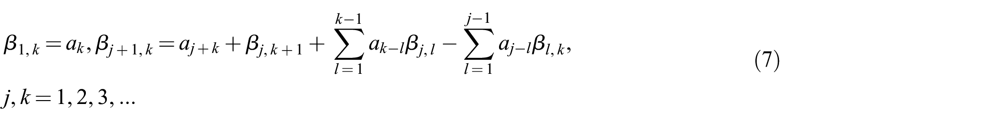
Here, the a_k (k = 1,2,3,…) in equation (7) are again given in the prescribed mapping (1). Since the Faber polynomials P_j(z) (j = 1,2,3,…) are defined in the entire region S₁, it is necessary to identify the corresponding range of validity of the argument $\xi$ in equation (6). Unfortunately, for over a decade this requirement has never been fully clarified in any of the relevant papers in this area where either the issue has been ignored completely (see studies [1–4]) or dealt with incorrectly (see Sudak [5] and McArthur and Sudak [6]). In particular, in Sudak [5] and McArthur and Sudak [6], the range of $\xi$ in equation (6) was mistakenly taken to be $\left|\xi \right|>1$ which does not, in fact, correspond to the domain of definition S₁ of the Faber polynomials but to some other region S₀ of the z-plane which makes no sense in the context of the physical problem. It is our opinion that the failure to clarify the range of $\xi$ in equation (6) may not only lead to further misunderstandings (see, for example, Chen [7] and Luo and Gao [8]) but also hinder further application of the Faber series to interesting problems in two-dimensional elasticity theory. In what follows, we seek to clarify the original form of Faber polynomials with emphasis on the origin of equation (6).

In fact, as suggested in Curtiss [9], if we multiply both sides of equation (2) by the term $(\omega (\xi )-z)$ and then compare coefficients of ${\xi }^{-j}$ (j = –1,0,1,2,3,…) on both sides of the resulting equation, it is not difficult to obtain the following recurrence relation:

$$P_{j+1}\left(z\right)=P_1\left(z\right)P_j\left(z\right)-\sum _{l=1}^{j-1}{a}_l{P}_{j-l}\left(z\right)-(j+1)a_j,j=1,2,3,...$$

(8)

with

$$P_0\left(z\right)=1,P_1\left(z\right)=\frac{z-z_0}{R}.$$

(9)

Here, from equations (8) and (9), it is clear that the Faber polynomial P_j(z) is no more than a jth order polynomial in z with leading term $(z-z_0{)}^j/R^j$ . When z lies on the curve L, it follows from the mapping (1) that

$$\begin{array}{c}z=\omega \left(\sigma \right)=z_0+R(\sigma +\sum _{k=1}^{+\infty }{a}_k{\sigma }^{-k}),\hfill \\ (z\in L,\sigma =e^{i\theta },0\le \theta <2\pi ).\hfill \end{array}$$

(10)

Substituting equation (10) into equations (8) and (9) results in the equation

$$P_j\left(z\right)={\sigma }^j+\sum _{k=1}^{+\infty }{\beta }_{j,k}{\sigma }^{-k},(z\in L,j=1,2,3,...),$$

(11)

where ${\beta }_{j,k}$ (j, k = 1,2,3,…) appear as exactly those introduced from equation (7). It is clear that to date, the so-called Faber polynomials (6) used in papers on this subject are, in fact, only the boundary values of the actual Faber polynomials (given by equations (8) and (9)) on the boundary L of S₁ in the z-plane. However, since the mapping (1) cannot generally associate the region S₁ in the z-plane with a specific region in the ξ-plane, it is not possible to derive a formula similar to equation (10) for a general point z inside S₁. Consequently, equation (6) is generally valid only when the argument $\xi$ falls on the unit circle in the ξ-plane so that it becomes necessary to use equations (8) and (9) to calculate the actual values of the Faber polynomials P_j(z) (j = 1,2,3,…) in the entire region S₁.

4. Replacement of the Faber series by Taylor series

In numerical investigations concerning the deformation of finite elastic bodies (see, for example, Dai et al. [11]), it is preferable to use truncated Faber series. Specifically, the unknown complex potential of an arbitrarily shaped elastic body (occupying a simply connected region S₁) is usually described (approximately) by a truncated Faber series as

$$f\left(z\right)=\sum _{j=0}^N{c}_j{P}_j\left(z\right),z\in S_1,$$

(12)

where c_j (j = 0,1,…)) are some unknown coefficients. Since each Faber polynomial P_j(z) in equation (12) is only an ordinary jth order polynomial with respect to z (see equations (8) and (9)), the truncated series (12) is equivalent to the following (truncated) “Taylor series”:

$$f\left(z\right)=\sum _{j=0}^N{d}_j{z}^j,z\in S_1,$$

(13)

where d_j (j = 0,1,…)) are some other unknown coefficients usually distinct from those in equation (12). Here, it is worth noting that when the number N of the truncated terms in the series (12) or (13) increases, the coefficients c_j (j = 0,1,2,…) determined from certain boundary conditions definitely converge while the coefficients d_j (j = 0,1,2,…) determined from the same boundary conditions usually do not. Despite this observation, for any given N, it follows from the equivalency of the series in equations (12) and (13) that the same function f(z) in the entire region S₁ will be obtained whether we use the series in equation (12) or that in equation (13). Consequently, when the emphasis of the investigation is on numerical analysis, it is reasonable to use Taylor series instead of the actual Faber series. In fact, the replacement of the Faber series by Taylor series has already been adopted in a number of related investigations (see, for example, studies [12–14]), although without a convincing explanation (such as the one presented here).

Finally, we mention that the idea of replacing Faber series with Taylor series is particularly useful when applying complex variable methods to two-dimensional anisotropic elasticity. In fact, for a finite anisotropic elastic body of given shape, since the domain of definition of its complex potential usually differs from the given physical region, it is generally difficult to derive the corresponding conformal mapping (1) for the domain of definition of the complex potential and thus give expressions for the corresponding Faber polynomials (as in equation (8)). Consequently, when complex variable methods are applied to the case of a finite anisotropic elastic body, the use of Taylor series in place of the Faber series is often more practical and convenient than in the corresponding case of isotropic elasticity.

5. Conclusions

We present a clarification of the use of Faber polynomials and Faber series with particular emphasis on their representation in both the original (physical) plane of definition and in the corresponding imaginary plane (defined via a conformal mapping). We note that in most of the associated published researches involving the complex potential of a finite elastic body, the so-called Faber series given in the imaginary plane, in fact, represents only the specific value of the complex potential on the boundary of the elastic body and cannot generally be used to describe the complex potential in the entire elastic body. We believe that such a clarification will serve to eliminate many of the misunderstandings and misinterpretations of the use of the Faber series in two-dimensional elasticity. In addition, we discuss the relationship between Faber series and Taylor series and show that truncated Faber series can indeed be simply replaced by truncated Taylor series without inducing any errors in the corresponding numerical analysis.