A general theory for anisotropic Kirchhoff–Love shells with in-plane bending of embedded fibers

Abstract

This work presents a generalized Kirchhoff–Love shell theory that can explicitly capture fiber-induced anisotropy not only in stretching and out-of-plane bending, but also in in-plane bending. This setup is particularly suitable for heterogeneous and fibrous materials such as textiles, biomaterials, composites and pantographic structures. The presented theory is a direct extension of classical Kirchhoff–Love shell theory to incorporate the in-plane bending resistance of fibers. It also extends existing second-gradient Kirchhoff–Love shell theory for initially straight fibers to initially curved fibers. To describe the additional kinematics of multiple fiber families, a so-called in-plane curvature tensor—which is symmetric and of second order—is proposed. The effective stress tensor and the in-plane and out-of-plane moment tensors are then identified from the mechanical power balance. These tensors are all second order and symmetric in general. Constitutive equations for hyperelastic materials are derived from different expressions of the mechanical power balance. The weak form is also presented as it is required for computational shell formulations based on rotation-free finite element discretizations. The proposed theory is illustrated by several analytical examples.

1. Introduction

Fiber-reinforced composites have become an important material in the sports, automotive, marine, and aerospace industry owing to their high-specific stiffness-to-weight ratio, which allows for lightweight designs. To produce such composites, fabric sheets are formed by warp and weft yarns (i.e. in a bundle of fibers) loosely linked together by different technologies, resulting, for example, in woven fabrics or non-crimp fabrics. The fabrics are then draped (molded) into desired shapes before injecting liquid resin (adhesives). After the resin solidifies, the fibers are strongly bonded together in the final product.

In this work, we are interested in continuum models for fabric sheets both with and without matrix material. Such models are required for the description and simulation of fiber-reinforced shell structures and draping processes. Geometrically, fabric structures can be modeled by a surface with embedded curves representing yarns. From the microscopic point of view, the resistance (in-plane and out-of-plane) of fabrics results from the deformation of yarns and their interaction, that is, their linkage and contact. In particular, axial stretching of fibers is associated with anisotropic membrane resistance, and the linkage between yarns offers shear resistance. Twisting of a yarn can be assumed to be fully associated with the second fundamental form of the yarn-embedding surface [1]. Bending of a yarn can have both in-plane and out-of-plane components and is characterized by the corresponding curvatures. The out-of-plane curvature is associated with the second fundamental form, while the in-plane curvature is associated with the gradient of the surface metric.

Fabric sheets can be modeled as thin shells from the macroscopic point of view, and Kirchhoff–Love kinematics together with plane stress conditions are usually adopted. Membrane deformation is characterized by stretching and shearing, while out-of-plane deformation is characterized by bending and twisting. In Kirchhoff–Love shell models, two kinematical quantities—the surface metric and the second fundamental form—are used for the two deformation types. In the literature, the general case of arbitrarily large deformations and nonlinear material behavior of shells has been treated extensively. See, for example, the texts of Naghdi [2], Pietraszkiewicz [3], Libai and Simmonds [4] and references therein. Here, we refer to this nonlinear case as classical Kirchhoff–Love shell theory. Note that although Kirchhoff–Love shell theory is mostly discussed for solids, its application can also be extended to liquid shells [5]. The incorporation of material anisotropy in classical Kirchhoff–Love shells due to embedded fibers—for both stretching and out-of-plane bending—is straightforward, see, for example, the works by Tepole et al. [6] and Wu et al. [7] and references therein. As shown by Roohbakhshan and Sauer [8], classical Kirchhoff–Love shell theory also admits complex anisotropic bending models, for example, due to fibers not located at the mid-surface.

While classical Kirchhoff–Love shell theory can also be regarded as a special case of Cosserat theory [9], ¹ it has its own development history and has the advantage of simplicity and intuitiveness when following its argument structure. Therefore, it facilitates building corresponding computational as well as physically based constitutive models. This motivated Sauer and Duong [10] to provide a unified formulation for both liquid and solid shells within the framework of classical Kirchhoff–Love shell theory. Their work aimed at providing a concise, yet general theoretical framework for corresponding computational rotation-free shell formulations [11,12].

It should be noted that most existing shell models, including classical Kirchhoff–Love shell theory, focus on out-of-plane bending, while the in-plane response is still based on the classical Cauchy continuum. That is, one assumes that there is no moment (or stress couple) causing in-plane bending at a material point. This assumption is usually sufficient when only the overall material behavior is of interest, as, for example, in the draping simulations of Khiêm et al. [13]. However, it fails to capture deformations governed by in-plane fiber bending, which are important for obtaining accurate and convergent numerical results. An example of these are the localized shear bands [14,15] in the bias-extension test. In this case, simulations with finite element shell models based on the in-plane Cauchy continuum will fail to converge to a finite width of the shear band under mesh refinement. Another example is the asymmetric deformation of woven fabrics with different in-plane fiber bending stiffness for different fiber families [16,17].

Similar effects of the in-plane bending stiffness can also be found in pantographic structures [18–20] and fibrous composites, such as biological tissues [21]. Thus, a more general model that considers the in-plane bending response is required for fabrics, fibrous composites, and pantographic structures.

The first theoretical work considering in-plane bending was presented by Wang and Pipkin [22,23] to model cloth and cable networks. Their theory is a special form of finite-deformation fibrous plate theory with inextensible fibers that contain bending couples that are proportional to their curvature. Since in-plane bending is related to the in-plane components of the second displacement gradient, it can be captured by more general continuum theories, such as Cosserat theories [24–26] and gradient theories [27–30]. For three-dimensional (3D) fiber-reinforced solids, Spencer and Soldatos [31] introduced explicitly the bending resistance of embedded fibers in the context of nonlinear second-gradient theory. A computational model based on Spencer and Soldatos [31] has been developed by Asmanoglo and Menzel [32]. Starting from Cosserat theory, Steigmann [33] derives a fiber-reinforced solid model that includes fiber bending, twisting, and stretching.

Concerned with in-plane bending for thin structures, Steigmann and Dell’Isola [1] presented a continuum model for woven fabric sheets modeled as orthotropic plates, which treats fibers as Kirchhoff–Love rods that are distributed continuously across the sheet. Although the concept of stress couples from Cosserat theory is used, the model of Steigmann and Dell’Isola [1] can be categorized as second-gradient theory, since their material model depends on the first and second displacement gradients. Following this, Steigmann [34] further developed a second-gradient shell model that explicitly includes general fiber bending, twisting, and stretching. There, a concise set of equilibrium equations, boundary conditions, and material symmetries are discussed. However, to the best of our knowledge, the theory has not yet been fully formulated for the general case of more than two fiber families with initially curved fibers.

Focusing on Kirchhoff–Love shells, Balobanov et al. [35] presented a new shell model derived from the second displacement gradient theory of Mindlin [28]. A corresponding computational formulation was also discussed in Balobanov et al. [35]. However, explicit in-plane fiber bending is not considered and the weak form requires at least $C^2$ -continuity of the geometry. Recently, Schulte et al. [36] applied the second-gradient theory of Steigmann [34] directly to Kirchhoff–Love shells and presented the first rotation-free computational shell formulation accounting for in-plane bending using $C^1$ -continuous discretization.

In this contribution, we propose a general Kirchhoff–Love shell theory that explicitly incorporates fiber bending (both in-plane and out-of-plane), geodesic fiber twisting, and stretching. Unlike the existing approaches that derive the Kirchhoff–Love shell from a more general theory, here our theory is constructed directly from Kirchhoff–Love thin shell assumptions without introducing extra degrees of freedom, such as independent directors or micro-displacements. It is shown that the in-plane fiber bending contribution can be formulated analogously to its out-of-plane counterpart. All the definitions of stresses and moments, and the equilibrium equations thus follow in the same manner as in classical Kirchhoff–Love shell theory. Unlike the second-gradient theory of Steigmann [34], the stress couple (or double force) in our theory is fully equivalent to the bending moment under Kirchhoff–Love assumptions.

Our approach provides several advantages over existing second-gradient shell theories, such as those of Steigmann and Dell’Isola [1] and Steigmann [34]. In particular, it allows us to identify work-conjugated pairs of symmetric stress and symmetric strain measures for all terms, including a new in-plane stress couple and corresponding in-plane curvature tensor. Instead of using third-order tensors for in-plane bending, as is done in current second-gradient shell theories, the stress and strain tensors in our theory are all of second order. Their invariants thus can be easily identified and geometrically interpreted, which is advantageous for constructing constitutive models. Furthermore, our theory admits a wide range of constitutive models for straight as well as initially curved fibers without limitation on the number of fiber families and the angles between them.

Besides, the presented work also aims at providing a general formulation that is suitable for a straightforward isogeometric finite element implementation [37]. Since the in-plane bending term in our theory is analogous to the out-of-plane bending term, existing finite element formulations for out-of-plane bending can be easily extended to in-plane bending. As for existing formulations, the corresponding weak form requires at least $C^1$ -continuous surface discretizations in the framework of rotation-free finite element formulations. For the purpose of verifying finite element implementations, we further provide the analytical solution for several nonlinear benchmark examples. Here, we are restricting ourselves to hyperelastic material models for the fabrics. Inelastic behavior, for example, due to inter- and intra-ply fiber sliding, will be considered in future work.

In summary, our approach contains the following novelties and merits compared to earlier works:

• A concise shell theory with in-plane bending that is a direct extension of classical Kirchhoff–Love thin shell theory;

• A general theory that can admit a wide range of constitutive models for straight or initially curved fibers with no limitation on the number of fiber families and the angles between them;

• The introduction of a new symmetric in-plane curvature tensor;

• The identification of work-conjugated pairs of symmetric stress and symmetric strain measures;

• The weak form as it is required for rotation-free finite element formulations;

• The analytical solution for several nonlinear benchmark examples that include different modes of fiber deformation and are useful for verifying computational formulations.

The following presentation is structured as follows: Section 2 summarizes the kinematics of thin shells with embedded curves and introduces the in-plane curvature tensor to capture the in-plane curvature of fibers. With this, the balance laws are presented in section 3. Different choices of work-conjugated pairs are then discussed in section 4. Section 5 gives some examples of constitutive models for the proposed theory. Section 6 then presents the weak form. Several analytical benchmark examples supporting the proposed theory are presented in section 7. The article is concluded by section 8.

2. Kinematics for thin shells with embedded curves

In this section, nonlinear Kirchhoff–Love shell kinematics [2] is extended to deforming surfaces with embedded curves. The extended kinematics allows to capture not only stretching and out-of-plane bending, but also in-plane bending of the embedded curves. Fiber-induced anisotropy is allowed in all these modes of deformation. The description is presented fully in the general framework of curvilinear coordinates. The variation of different kinematical quantities can be found in Appendix 2.

2.1. Geometric description

The mid-surface of a thin shell at time $t$ is modeled in three-dimensional space as a two-dimensional (2D) manifold, denoted by $\mathcal{S}$ . In curvilinear coordinates, $\mathcal{S}$ is described by the one-to-one mapping of a point $({\xi }^1,{\xi }^2)$ in parameter space $\mathcal{P}$ to the point $\mathit{x}\in \mathcal{S}$ as

$$\mathit{x}=\mathit{x}({\xi }^{\alpha },t),\mathrm{with}\alpha =1,2.$$

(1)

The (covariant) tangent vectors along the convective coordinate curves ${\xi }^{\alpha }$ at any point $\mathit{x}\in \mathcal{S}$ can be defined by

$${\mathit{a}}_{\alpha }:=\frac{\partial \mathit{x}}{\partial {\xi }^{\alpha }}={\mathit{x}}_{,\alpha },$$

(2)

where the comma denotes the parametric derivative. The unit normal vector can then be defined by

$$\mathit{n}:=\frac{{\mathit{a}}_1\times {\mathit{a}}_2}{\parallel {\mathit{a}}_1\times {\mathit{a}}_2\parallel }.$$

(3)

From the tangent vectors ${\mathit{a}}_{\alpha }$ in equation (2), the so-called dual tangent vectors, denoted by ${\mathit{a}}^{\alpha }$ , are defined by

$${\mathit{a}}^{\alpha }·{\mathit{a}}_{\beta }={\delta }_{\beta }^{\alpha },$$

(4)

with ${\delta }_{\beta }^{\alpha }$ being the Kronecker delta. The covariant and dual tangent vectors are related to each other by ² ${\mathit{a}}_{\alpha }=a_{\alpha \beta }{\mathit{a}}^{\beta }$ and ${\mathit{a}}^{\alpha }=a^{\alpha \beta }{\mathit{a}}_{\beta }$ , where

$$\begin{array}{c}{a}_{\alpha \beta }:={\mathit{a}}_{\alpha }·{\mathit{a}}_{\beta },a^{\alpha \beta }:={\mathit{a}}^{\alpha }·{\mathit{a}}^{\beta }\hfill \end{array}$$

(5)

denote the co- and contravariant surface metric, respectively.

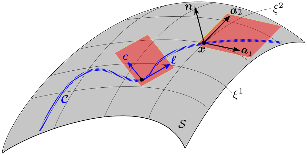
Furthermore, in order to model fibrous thin shells, a fiber (or a bundle of fibers) is geometrically represented by a curve $\mathcal{C}$ defined by the points $\mathit{x}={\mathit{x}}_{\mathrm{c}}(s,t)$ , with $\mathrm{d}s=\parallel \mathrm{d}\mathit{x}\parallel$ , embedded in surface $\mathcal{S}$ (see Figure 1). The distribution of fibers is considered continuous such that a homogenized shell theory is obtained. The normalized tangent vector of $\mathcal{C}$ , defined by

$$\mathit{\ell }:=\frac{\partial {\mathit{x}}_{\mathrm{c}}}{\partial s}={\mathit{\ell }}_{\alpha }{\mathit{a}}^{\alpha }={\mathit{\ell }}^{\alpha }{\mathit{a}}_{\alpha },$$

(6)

represents the fiber direction at location $s$ . Here, ${\ell }_{\alpha }:=\mathit{\ell }·{\mathit{a}}_{\alpha }$ and ${\ell }^{\alpha }:=\mathit{\ell }·{\mathit{a}}^{\alpha }$ denote the covariant and contravariant components of vector $\mathit{\ell }$ in the convective coordinate system, respectively. Assuming that the deformation of fibers satisfies Euler–Bernoulli kinematics, the in-plane director for the fiber $\mathcal{C}$ can be defined by

$$\begin{array}{c}\mathit{c}:=\mathit{n}\times \mathit{\ell }=c_{\alpha }{\mathit{a}}^{\alpha }=c^{\alpha }{\mathit{a}}_{\alpha },\hfill \end{array}$$

(7)

where, $c_{\alpha }:=\mathit{c}·{\mathit{a}}_{\alpha }$ and $c^{\alpha }:=\mathit{c}·{\mathit{a}}^{\alpha }$ are the covariant and contravariant components of vector $\mathit{c}$ , respectively. With equations (6) and (7), bases $\{{\mathit{a}}_1,{\mathit{a}}_2,\mathit{n}\}$ and $\{{\mathit{a}}^1,{\mathit{a}}^2,\mathit{n}\}$ can be represented by the local Cartesian basis $\{\mathit{\ell },\mathit{c},\mathit{n}\}$ as

$$\begin{array}{c}{\mathit{a}}_{\alpha }={\ell }_{\alpha }\mathit{\ell }+c_{\alpha }\mathit{c},\mathrm{and}{\mathit{a}}^{\alpha }={\mathit{\ell }}^{\alpha }\mathit{\ell }+c^{\alpha }\mathit{c}.\hfill \end{array}$$

(8)

Figure 1.

A fiber bundle represented by curve $\mathcal{C}$ is embedded in shell surface $\mathcal{S}$ . The red planes illustrate tangent planes.

The surface identity tensor $\mathit{i}$ and the full identity $1$ in ${\mathbb{R}}^3$ can then be written as

$$\begin{array}{c}\mathit{i}:={\mathit{a}}_{\alpha }\otimes {\mathit{a}}^{\alpha }={\mathit{a}}^{\alpha }\otimes {\mathit{a}}_{\alpha }=\mathit{c}\otimes \mathit{c}+\mathit{\ell }\otimes \mathit{\ell },\hfill \end{array}$$

(9)

and

$$\begin{array}{c}1=\mathit{i}+\mathit{n}\otimes \mathit{n}.\hfill \end{array}$$

(10)

2.2. Surface curvature

The curvature of surface $\mathcal{S}$ can be described by the symmetric second-order tensor

$$\begin{array}{c}\mathit{b}:=b_{\alpha \beta }{\mathit{a}}^{\alpha }\otimes {\mathit{a}}^{\beta }=b_{\alpha }^{\beta }{\mathit{a}}^{\alpha }\otimes {\mathit{a}}_{\beta }=b^{\alpha \beta }{\mathit{a}}_{\alpha }\otimes {\mathit{a}}_{\beta }.\hfill \end{array}$$

(11)

The components $b_{\alpha \beta }$ can be computed from the derivative of surface normal $\mathit{n}$ as

$$\begin{array}{c}{b}_{\alpha \beta }:=-{\mathit{n}}_{,\alpha }·{\mathit{a}}_{\beta },\hfill \end{array}$$

(12)

which leads to Weingarten’s formula

$$\begin{array}{c}{\mathit{n}}_{,\alpha }=-b_{\alpha \beta }{\mathit{a}}^{\beta }.\hfill \end{array}$$

(13)

Alternatively, components $b_{\alpha \beta }$ can be extracted from the derivatives of tangent vectors ${\mathit{a}}_{\alpha }$ as

$$\begin{array}{c}{b}_{\alpha \beta }:=\mathit{n}·{\mathit{a}}_{\alpha ,\beta }=\mathit{n}·{\mathit{a}}_{\alpha ;\beta },\hfill \end{array}$$

(14)

where

$${\mathit{a}}_{\alpha ,\beta }:=\frac{\partial {\mathit{a}}_{\alpha }}{\partial {\xi }^{\beta }}={\mathit{x}}_{,\alpha \beta },\mathrm{and}{\mathit{a}}_{\alpha ;\beta }:=(\mathit{n}\otimes \mathit{n}){\mathit{a}}_{\alpha ,\beta }=b_{\alpha \beta }\mathit{n}$$

(15)

are the parametric and covariant derivative of ${\mathit{a}}_{\alpha }$ , respectively. ³

Unlike ${\mathit{n}}_{,\alpha }$ , which always lies in the tangent plane, ${\mathit{a}}_{\alpha ,\beta }$ can have both tangential and normal components. With respect to basis $\{{\mathit{a}}_1,{\mathit{a}}_2,\mathit{n}\}$ the vectors ${\mathit{a}}_{\alpha ,\beta }$ can be expressed as

$$\begin{array}{c}{\mathit{a}}_{\alpha ,\beta }={\mathrm{\Gamma }}_{\alpha \beta }^{\gamma }{\mathit{a}}_{\gamma }+b_{\alpha \beta }\mathit{n},\hfill \end{array}$$

(16)

where the tangential components

$$\begin{array}{c}{\mathrm{\Gamma }}_{\alpha \beta }^{\gamma }:={\mathit{a}}_{\alpha ,\beta }·{\mathit{a}}^{\gamma }\hfill \end{array}$$

(17)

are known as the surface Christoffel symbols. They are symmetric in indices $\alpha$ and $\beta$ . Using transformation (8.2), they can be expressed as

$$\begin{array}{c}{\mathrm{\Gamma }}_{\alpha \beta }^{\gamma }=c^{\gamma }{\mathrm{\Gamma }}_{\alpha \beta }^{\mathrm{c}}+{\ell }^{\gamma }{\mathrm{\Gamma }}_{\alpha \beta }^{\ell },\hfill \end{array}$$

(18)

where we have defined

$$\begin{array}{c}{\mathrm{\Gamma }}_{\alpha \beta }^{\mathrm{c}}:=\mathit{c}·{\mathit{a}}_{\alpha ,\beta }=c_{\gamma }{\mathrm{\Gamma }}_{\alpha \beta }^{\gamma },\hfill \\ \multicolumn{1}{c}{{\mathrm{\Gamma }}_{\alpha \beta }^{\ell }:=\mathit{\ell }·{\mathit{a}}_{\alpha ,\beta }={\mathit{\ell }}_{\gamma }{\mathrm{\Gamma }}_{\alpha \beta }^{\gamma }.}\end{array}$$

(19)

The curvature tensor $\mathit{b}$ defined in equation (11) has the two invariants

$$H:=\frac{1}{2}\mathrm{t}{\mathrm{r}}_{\mathrm{s}}\mathit{b}=\frac{1}{2}{b}_{\alpha }^{\alpha },\mathrm{and}\kappa ={det}_{\mathrm{s}}\mathit{b}:=det[b_{\alpha }^{\beta }].$$

(20)

They correspond to the mean and Gaussian curvatures, respectively. The curvature tensor $\mathit{b}$ fully describes the out-of-plane curvature of surface $\mathcal{S}$ . Thus, we can extract from it the curvature of $\mathcal{S}$ along any direction. For example,

$$\begin{array}{c}{\kappa }_{\mathrm{n}}:=\mathit{b}:\mathit{\ell }\otimes \mathit{\ell }=b_{\alpha \beta }{\ell }^{\alpha \beta },\mathrm{with}{\ell }^{\alpha \beta }:={\ell }^{\alpha }{\ell }^{\beta },\hfill \end{array}$$

(21)

represents the curvature of $\mathcal{S}$ in direction $\mathit{\ell }$ . Hence, ${\kappa }_{\mathrm{n}}$ also expresses the so-called normal curvature of the curve $\mathcal{C}$ embedded in $\mathcal{S}$ . Furthermore,

$$\begin{array}{c}{\tau }_{\mathrm{g}}:=\mathit{b}:\mathit{\ell }\otimes \mathit{c}=\mathit{b}:\mathit{c}\otimes \mathit{\ell }=b_{\alpha \beta }{\ell }^{\alpha }{c}^{\beta },\hfill \end{array}$$

(22)

denotes the so-called geodesic torsion of $\mathcal{C}$ .

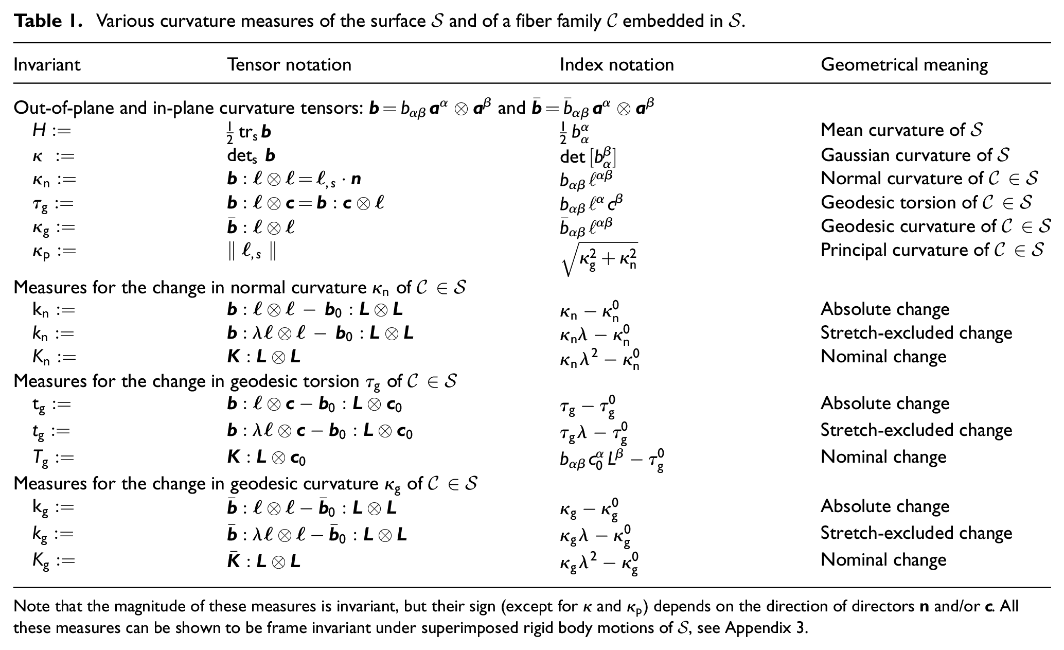
The mentioned invariants $H$ , $\kappa$ , ${\kappa }_{\mathrm{n}}$ , and ${\tau }_{\mathrm{g}}$ are included in Table 1. They are useful in constructing material models for (both isotropic and anisotropic) out-of-plane bending.

Table 1.

Various curvature measures of the surface $\mathcal{S}$ and of a fiber family $\mathcal{C}$ embedded in $\mathcal{S}$ .

Invariant	Tensor notation	Index notation	Geometrical meaning
Out-of-plane and in-plane curvature tensors: $\mathit{b}=b_{\alpha \beta }{\mathit{a}}^{\alpha }\otimes {\mathit{a}}^{\beta }$ and $\overline{\mathit{b}}={\overline{b}}_{\alpha \beta }{\mathit{a}}^{\alpha }\otimes {\mathit{a}}^{\beta }$
$H:=$	$\frac{1}{2}\mathrm{t}{\mathrm{r}}_{\mathrm{s}}\mathit{b}$	$\frac{1}{2}{b}_{\alpha }^{\alpha }$	Mean curvature of $\mathcal{S}$
$\kappa :=$	$\underset{\mathrm{s}}{det}\mathit{b}$	$det[b_{\alpha }^{\beta }]$	Gaussian curvature of $\mathcal{S}$
${\kappa }_{\mathrm{n}}:=$	$\mathit{b}:\mathit{\ell }\otimes \mathit{\ell }={\mathit{\ell }}_{,s}·\mathit{n}$	$b_{\alpha \beta }{\ell }^{\alpha \beta }$	Normal curvature of $\mathcal{C}\in \mathcal{S}$
${\tau }_{\mathrm{g}}:=$	$\mathit{b}:\mathit{\ell }\otimes \mathit{c}=\mathit{b}:\mathit{c}\otimes \mathit{\ell }$	$b_{\alpha \beta }{\ell }^{\alpha }{c}^{\beta }$	Geodesic torsion of $\mathcal{C}\in \mathcal{S}$
${\kappa }_{\mathrm{g}}:=$	$\overline{\mathit{b}}:\mathit{\ell }\otimes \mathit{\ell }$	${\overline{b}}_{\alpha \beta }{\ell }^{\alpha \beta }$	Geodesic curvature of $\mathcal{C}\in \mathcal{S}$
${\kappa }_{\mathrm{p}}:=$	$\parallel {\mathit{\ell }}_{,s}\parallel$	$\sqrt{{\kappa }_{\mathrm{g}}^2+{\kappa }_{\mathrm{n}}^2}$	Principal curvature of $\mathcal{C}\in \mathcal{S}$
Measures for the change in normal curvature ${\kappa }_{\mathrm{n}}$ of $\mathcal{C}\in \mathcal{S}$
${\mathrm{k}}_{\mathrm{n}}:=$	$\mathit{b}:\mathit{\ell }\otimes \mathit{\ell }-{\mathit{b}}_0:\mathit{L}\otimes \mathit{L}$	${\kappa }_{\mathrm{n}}-{\kappa }_{\mathrm{n}}^0$	Absolute change
$k_{\mathrm{n}}:=$	$\mathit{b}:\lambda \mathit{\ell }\otimes \mathit{\ell }-{\mathit{b}}_0:\mathit{L}\otimes \mathit{L}$	${\kappa }_{\mathrm{n}}\lambda -{\kappa }_{\mathrm{n}}^0$	Stretch-excluded change
$K_{\mathrm{n}}:=$	$\mathit{K}:\mathit{L}\otimes \mathit{L}$	${\kappa }_{\mathrm{n}}{\lambda }^2-{\kappa }_{\mathrm{n}}^0$	Nominal change
Measures for the change in geodesic torsion ${\tau }_{\mathrm{g}}$ of $\mathcal{C}\in \mathcal{S}$
${\mathrm{t}}_{\mathrm{g}}:=$	$\mathit{b}:\mathit{\ell }\otimes \mathit{c}-{\mathit{b}}_0:\mathit{L}\otimes {\mathit{c}}_0$	${\tau }_{\mathrm{g}}-{\tau }_{\mathrm{g}}^0$	Absolute change
$t_{\mathrm{g}}:=$	$\mathit{b}:\lambda \mathit{\ell }\otimes \mathit{c}-{\mathit{b}}_0:\mathit{L}\otimes {\mathit{c}}_0$	${\tau }_{\mathrm{g}}\lambda -{\tau }_{\mathrm{g}}^0$	Stretch-excluded change
$T_{\mathrm{g}}:=$	$\mathit{K}:\mathit{L}\otimes {\mathit{c}}_0$	$b_{\alpha \beta }{c}_0^{\alpha }{L}^{\beta }-{\tau }_{\mathrm{g}}^0$	Nominal change
Measures for the change in geodesic curvature ${\kappa }_{\mathrm{g}}$ of $\mathcal{C}\in \mathcal{S}$
${\mathrm{k}}_{\mathrm{g}}:=$	$\overline{\mathit{b}}:\mathit{\ell }\otimes \mathit{\ell }-{\overline{\mathit{b}}}_0:\mathit{L}\otimes \mathit{L}$	${\kappa }_{\mathrm{g}}-{\kappa }_{\mathrm{g}}^0$	Absolute change
$k_{\mathrm{g}}:=$	$\overline{\mathit{b}}:\lambda \mathit{\ell }\otimes \mathit{\ell }-{\overline{\mathit{b}}}_0:\mathit{L}\otimes \mathit{L}$	${\kappa }_{\mathrm{g}}\lambda -{\kappa }_{\mathrm{g}}^0$	Stretch-excluded change
$K_{\mathrm{g}}:=$	$\overline{\mathit{K}}:\mathit{L}\otimes \mathit{L}$	${\kappa }_{\mathrm{g}}{\lambda }^2-{\kappa }_{\mathrm{g}}^0$	Nominal change

Note that the magnitude of these measures is invariant, but their sign (except for $\kappa$ and ${\kappa }_{\mathrm{p}}$ ) depends on the direction of directors $n$ and/or $\mathit{c}$ . All these measures can be shown to be frame invariant under superimposed rigid body motions of $\mathcal{S}$ , see Appendix 3.

2.3. Curvature of embedded curves

We aim at capturing any geodesic torsion, normal and in-plane curvature of an embedded curve $\mathcal{C}\in \mathcal{S}$ . As seen in equations (21) and (22), the normal curvature and geodesic torsion of $\mathcal{C}$ can already be described via the out-of-plane curvature tensor (11). The in-plane curvature, on the other hand, does not follow from tensor $\mathit{b}$ . Instead, it can be extracted from the so-called curvature vector of $\mathcal{C}$ that is defined by the directional derivative of $\mathit{\ell }$ in direction $\mathit{\ell }$ , that is,

$${\mathit{\ell }}_{,s}:=\frac{\partial \mathit{\ell }}{\partial s}=({\nabla }_{\mathrm{s}}\mathit{\ell })\mathit{\ell }={\mathit{\ell }}^{\alpha }{\mathit{\ell }}_{,\alpha }.$$

(23)

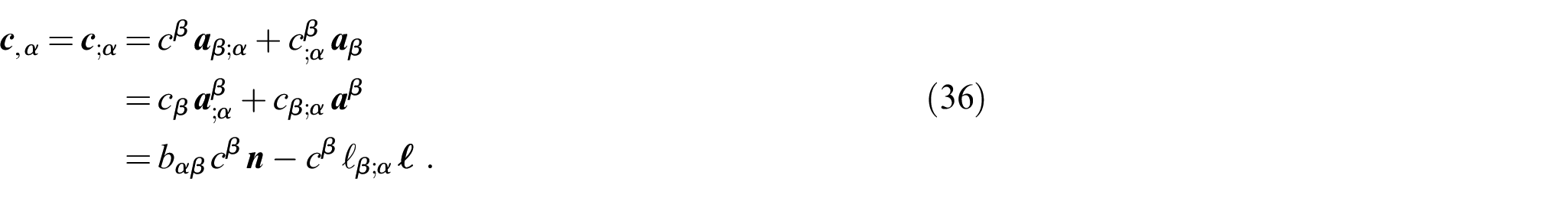
Here and henceforth, ${\nabla }_{\mathrm{s}}•:={•}_{,\alpha }\otimes {\mathit{a}}^{\alpha }$ denotes the surface gradient operator. ⁴ Following equation (6) and considering equations (4) and (16), derivative ${\mathit{\ell }}_{,\alpha }$ can be expressed as

$${\mathit{\ell }}_{,\alpha }={\ell }_{;\alpha }^{\beta }{\mathit{a}}_{\beta }+{\ell }^{\beta }{b}_{\beta \alpha }\mathit{n}={\ell }_{\beta ;\alpha }{\mathit{a}}^{\beta }+{\ell }^{\beta }{b}_{\beta \alpha }\mathit{n},$$

(24)

where the semicolon denotes the covariant derivatives

$$\begin{array}{c}{\ell }_{;\alpha }^{\beta }:={\mathit{\ell }}_{,\alpha }·{\mathit{a}}^{\beta }={\ell }_{,\alpha }^{\beta }+{\ell }^{\gamma }{\mathrm{\Gamma }}_{\gamma \alpha }^{\beta },\hfill \\ \multicolumn{1}{c}{{\ell }_{\beta ;\alpha }:={\mathit{\ell }}_{,\alpha }·{\mathit{a}}_{\beta }={\ell }_{\beta ,\alpha }-{\ell }_{\gamma }{\mathrm{\Gamma }}_{\beta \alpha }^{\gamma }.}\end{array}$$

(25)

The magnitude $\parallel {\mathit{\ell }}_{,s}\parallel =:{\kappa }_{\mathrm{p}}$ is called the principal curvature of $\mathcal{C}$ , ⁵ and the direction ${\mathit{\ell }}_{,s}/{\kappa }_{\mathrm{p}}=:{\mathit{n}}_{\mathrm{p}}$ is referred to as the principal normal to $\mathcal{C}$ . Note that ${\mathit{n}}_{\mathrm{p}}$ is normal to the curve but not necessarily normal to the surface $\mathcal{S}$ .

In principle, vector ${\mathit{\ell }}_{,s}$ can be expressed in any basis, which then induces different curvatures from the corresponding components. Here, we express ${\mathit{\ell }}_{,s}$ in the basis $\{\mathit{\ell },c,n\}$ , that is,

$$\begin{array}{c}{\mathit{\ell }}_{,s}={\kappa }_{\mathrm{p}}{\mathit{n}}_{\mathrm{p}}={\kappa }_{\mathrm{g}}\mathit{c}+{\kappa }_{\mathrm{n}}\mathit{n},\hfill \end{array}$$

(26)

where

$${\kappa }_{\mathit{n}}:=n·{\mathit{\ell }}_{,s},$$

(27)

denotes the normal curvature of $\mathcal{C}$ . By inserting equations (23) and (24), ${\kappa }_{\mathrm{n}}$ can be shown to be identical to equation (21). On the other hand,

$$\begin{array}{c}{\kappa }_{\mathrm{g}}:=\mathit{c}·{\mathit{\ell }}_{,s}\hfill \end{array}$$

(28)

is the in-plane (i.e. geodesic) curvature of $\mathcal{C}$ . It can be computed by inserting equations (23) and (24) into equation (28), giving

$$\begin{array}{c}{\kappa }_{\mathrm{g}}={\ell }_{\alpha ;\beta }{c}^{\alpha }{\ell }^{\beta }={\ell }_{;\beta }^{\alpha }{c}_{\alpha }{\ell }^{\beta }=({\overline{\nabla }}_{\mathrm{s}}\mathit{\ell }):\mathit{c}\otimes \mathit{\ell },\hfill \end{array}$$

(29)

where

$$\begin{array}{c}{\overline{\nabla }}_{\mathrm{s}}\mathit{\ell }:=\mathit{i}{\nabla }_{\mathrm{s}}\mathit{\ell }={\mathit{\ell }}_{\alpha ;\beta }{\mathit{a}}^{\alpha }\otimes {\mathit{a}}^{\beta }={\mathit{\ell }}_{;\beta }^{\alpha }{\mathit{a}}_{\alpha }\otimes {\mathit{a}}^{\beta }\hfill \end{array}$$

(30)

denotes the projected surface gradient of $\mathit{\ell }$ . ⁶

Remark 2.1. From equation (26) follows

$${\kappa }_{\mathrm{p}}^2={\kappa }_{\mathrm{g}}^2+{\kappa }_{\mathrm{n}}^2.$$

(31)

Remark 2.2. The three scalars ${\kappa }_{\mathrm{n}}$ , ${\kappa }_{\mathrm{g}}$ , and ${\tau }_{\mathrm{g}}$ are associated with the three bending modes of $\mathcal{C}\in \mathcal{S}$ : normal (i.e. out-of-plane) bending, geodesic (i.e. in-plane) bending, and geodesic torsion, respectively.

2.4. Definition of the in-plane curvature tensor

In principle, we can use the second-order tensor ${\overline{\nabla }}_{\mathrm{s}}\mathit{\ell }$ to characterize the in-plane curvature as the counterpart to tensor $\mathit{b}$ from equation (11), which characterizes the out-of-plane curvature. Tensor ${\overline{\nabla }}_{\mathrm{s}}\mathit{\ell }$ is, however, unsymmetric. We thus construct an alternative tensor by rewriting equation (29) and using identity ${\mathit{c}}_{,s}·\mathit{\ell }=-\mathit{c}·{\mathit{\ell }}_{,s}$ that follows from $\mathit{c}·\mathit{\ell }=0$ , so that

$$\begin{array}{c}{\kappa }_{\mathrm{g}}:=-{\ell }_{\alpha }^{\beta }{c}_{;\beta }^{\alpha }=-{\ell }^{\alpha \beta }{c}_{\alpha ;\beta }=\overline{\mathit{b}}:\mathit{\ell }\otimes \mathit{\ell },\hfill \end{array}$$

(32)

where

$$c_{;\alpha }^{\beta }:=c_{,\alpha }^{\beta }+c^{\gamma }{\mathrm{\Gamma }}_{\gamma \alpha }^{\beta },\mathrm{and}{c}_{\beta ;\alpha }:=c_{\beta ,\alpha }-c_{\gamma }{\mathrm{\Gamma }}_{\beta \alpha }^{\gamma },$$

(33)

similar to equation (25). Here, we have defined the so-called in-plane curvature tensor of $\mathcal{C}$ as

$$\begin{array}{c}\overline{\mathit{b}}:=-\frac{1}{2}[{\overline{\nabla }}_{\mathrm{s}}\mathit{c}+{({\overline{\nabla }}_{\mathrm{s}}\mathit{c})}^{\mathrm{T}}]=-\frac{1}{2}(c_{\alpha ;\beta }+c_{\beta ;\alpha }){\mathit{a}}^{\alpha }\otimes {\mathit{a}}^{\beta }={\overline{b}}_{\alpha \beta }{\mathit{a}}^{\alpha }\otimes {\mathit{a}}^{\beta }.\hfill \end{array}$$

(34)

Components ${\overline{b}}_{\alpha \beta }$ thus can be computed from

$$\begin{array}{c}{\overline{b}}_{\alpha \beta }=\overline{\mathit{b}}:{\mathit{a}}_{\alpha }\otimes {\mathit{a}}_{\beta }=-\frac{1}{2}(c_{\alpha ;\beta }+c_{\beta ;\alpha })=-\frac{1}{2}({\mathit{c}}_{,\alpha }·{\mathit{a}}_{\beta }+{\mathit{c}}_{,\beta }·{\mathit{a}}_{\alpha }),\hfill \end{array}$$

(35)

where

$$\begin{array}{c}\multicolumn{1}{c}{{\mathit{c}}_{,\alpha }={\mathit{c}}_{;\alpha }=c^{\beta }{\mathit{a}}_{\beta ;\alpha }+c_{;\alpha }^{\beta }{\mathit{a}}_{\beta }}\\ \multicolumn{1}{c}{=c_{\beta }{\mathit{a}}_{;\alpha }^{\beta }+c_{\beta ;\alpha }{\mathit{a}}^{\beta }}\\ \multicolumn{1}{c}{=b_{\alpha \beta }{c}^{\beta }\mathit{n}-c^{\beta }{\ell }_{\beta ;\alpha }\mathit{\ell }.}\end{array}$$

(36)

The last equation is obtained from identities $\mathit{c}·\mathit{n}=0$ , $\mathit{\ell }·\mathit{n}=0$ , and equations (24) and (13). The quantities ${\overline{b}}_{\alpha \beta }$ , ${\kappa }_{\mathrm{g}}$ , $c_{\beta ;\alpha }$ , and ${\ell }_{\beta ;\alpha }$ can be shown to be frame invariant under superimposed rigid body motions of $\mathcal{S}$ , see Appendix 3.

Remark 2.3. Since vector $\mathit{\ell }$ is normalized, we have the identity

$$\mathit{\ell }·{\mathit{\ell }}_{,\alpha }={\mathit{\ell }}_{\beta }{\mathit{\ell }}_{;\alpha }^{\beta }={\mathit{\ell }}^{\beta }{\mathit{\ell }}_{\beta ;\alpha }=0,$$

(37)

due to equation (24). Furthermore, equating equations (29) and (32) gives the relation

$${\ell }^{\beta }{c}_{\beta ;\alpha }=-c^{\beta }{\ell }_{\beta ;\alpha },$$

(38)

and from equation (36), we find

$$\begin{array}{c}{c}_{\beta ;\alpha }={\mathit{a}}_{\beta }·c_{,\alpha }=-c^{\gamma }{\ell }_{\beta }{\ell }_{\gamma ;\alpha }\hfill \\ \multicolumn{1}{c}{c_{;\alpha }^{\beta }={\mathit{a}}^{\beta }·c_{,\alpha }=-c^{\gamma }{\ell }^{\beta }{\ell }_{\gamma ;\alpha }.}\end{array}$$

(39)

2.5. Shell deformation

To characterize the shell deformation, a reference configuration ${\mathcal{S}}_0$ is chosen. The tangent vectors ${\mathit{A}}_{\alpha }$ , the normal vector $\mathit{N}$ , the surface metric $A_{\alpha \beta }$ , the out-of-plane curvature tensor ${\mathit{b}}_0:=B_{\alpha \beta }{\mathit{A}}^{\alpha }\otimes {\mathit{A}}^{\beta }$ are defined on ${\mathcal{S}}_0$ similar to equations (2), (3), (5), and (11), respectively.The fiber embedded within the shell surface is denoted by ${\mathcal{C}}_0$ in the reference configuration. Also, the normalized fiber direction $\mathit{L}=L^{\alpha }{\mathit{A}}_{\alpha }=L_{\alpha }{\mathit{A}}^{\alpha }$ , the in-plane fiber director ${\mathit{c}}_0=c_{\alpha }^0{\mathit{A}}^{\alpha }$ , and the in-plane curvature tensor ${\overline{\mathit{b}}}_0:={\overline{B}}_{\alpha \beta }{\mathit{A}}^{\alpha }\otimes {\mathit{A}}^{\beta }=-\frac{1}{2}(c_{\alpha ;\beta }^0+c_{\beta ;\alpha }^0){\mathit{A}}^{\alpha }\otimes {\mathit{A}}^{\beta }$ are defined similar to equations (6), (7), and (34), respectively.

Having $a_{\alpha \beta }$ , $b_{\alpha \beta }$ , and ${\overline{b}}_{\alpha \beta }$ the deformation of a shell can now be characterized by the following three tensors:

• 1. The surface deformation gradient:

$$\begin{array}{c}\mathit{F}:={\mathit{a}}_{\alpha }\otimes {\mathit{A}}^{\alpha }.\hfill \end{array}$$

(40)

This tensor can be used to map the reference fiber direction $\mathit{L}$ to $\mathit{\ell }$ as

$$\begin{array}{c}\lambda \mathit{\ell }=\mathit{F}\mathit{L}=L^{\alpha }{\mathit{a}}_{\alpha },\hfill \end{array}$$

(41)

where $\lambda$ is the fiber stretch. Comparing equations (6) and (41) gives

$$\begin{array}{c}{\ell }^{\alpha }=L^{\alpha }{\lambda }^{-1}.\hfill \end{array}$$

(42)

From (25) and (42) follows that

$${\ell }_{\alpha ;\beta }={\hat{L}}_{\alpha ,\beta }-{\ell }_{\alpha \gamma }({\hat{L}}_{,\beta }^{\gamma }+{\ell }^{\delta }{\mathrm{\Gamma }}_{\delta \beta }^{\gamma })+{\ell }^{\gamma }{\mathit{a}}_{\alpha }·{\mathit{a}}_{\gamma ,\beta },$$

(43)

where

$$\begin{array}{c}{\hat{L}}_{,\beta }^{\alpha }:={\lambda }^{-1}{L}_{,\beta }^{\alpha },\mathrm{and}{\hat{L}}_{\alpha ,\beta }:=a_{\alpha \gamma }{\hat{L}}_{,\beta }^{\gamma }.\hfill \end{array}$$

(44)

Inserting (43) into equation (39) gives

$$\begin{array}{c}{c}_{\beta ;\alpha }=-{\ell }_{\beta }(c^{\gamma }{\hat{L}}_{\gamma ,\alpha }+{\ell }^{\gamma }{\mathrm{\Gamma }}_{\gamma \alpha }^{\mathrm{c}}),\hfill \\ \multicolumn{1}{c}{c_{;\alpha }^{\beta }=-{\ell }^{\beta }(c^{\gamma }{\hat{L}}_{\gamma ,\alpha }+{\ell }^{\gamma }{\mathrm{\Gamma }}_{\gamma \alpha }^{\mathrm{c}}).}\end{array}$$

(45)

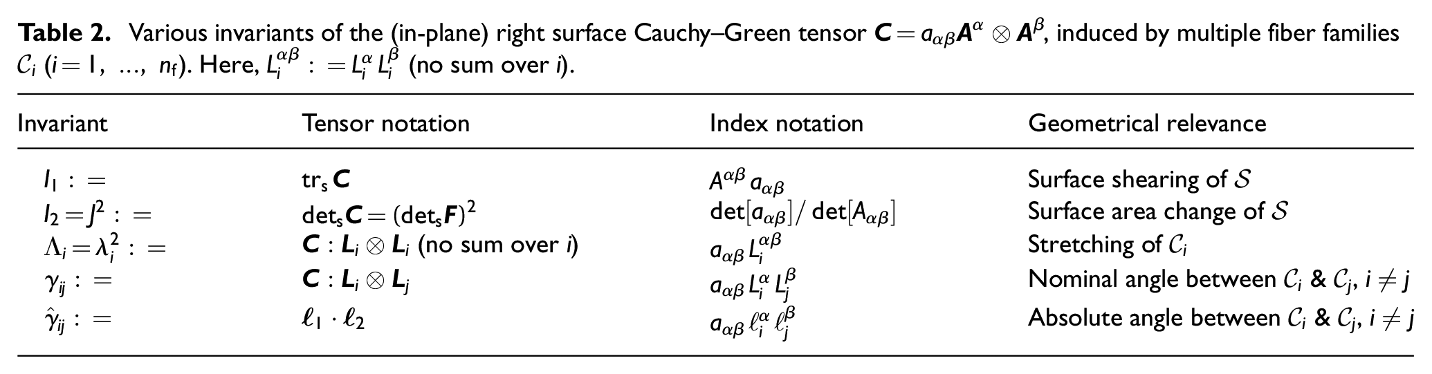
With the surface deformation gradient, the right Cauchy–Green surface tensor is defined by $\mathit{C}:={\mathit{F}}^{\mathrm{T}}\mathit{F}=a_{\alpha \beta }{\mathit{A}}^{\alpha }\otimes {\mathit{A}}^{\beta }$ . Table 2 lists some invariants induced by $\mathit{C}$ that can be useful for constructing material models. The Green–Lagrange surface strain tensor, which represents the change of the surface metric, is then defined by

$$\begin{array}{c}\mathit{E}:=\frac{1}{2}(\mathit{C}-\mathit{I})=\frac{1}{2}(a_{\alpha \beta }-A_{\alpha \beta }){\mathit{A}}^{\alpha }\otimes {\mathit{A}}^{\beta }=E_{\alpha \beta }{\mathit{A}}^{\alpha }\otimes {\mathit{A}}^{\beta }.\hfill \end{array}$$

(46)

• 2. The change of the out-of-plane curvature tensor:

$$\begin{array}{c}\mathit{K}:={\mathit{F}}^T\mathit{b}\mathit{F}-{\mathit{b}}_0=(b_{\alpha \beta }-B_{\alpha \beta }){\mathit{A}}^{\alpha }\otimes {\mathit{A}}^{\beta }=K_{\alpha \beta }{\mathit{A}}^{\alpha }\otimes {\mathit{A}}^{\beta }.\hfill \end{array}$$

(47)

• 3. The change of the in-plane curvature tensor:

$$\begin{array}{c}\overline{\mathit{K}}:={\mathit{F}}^T\overline{\mathit{b}}\mathit{F}-{\overline{\mathit{b}}}_0=({\overline{b}}_{\alpha \beta }-{\overline{B}}_{\alpha \beta }){\mathit{A}}^{\alpha }\otimes {\mathit{A}}^{\beta }={\overline{K}}_{\alpha \beta }{\mathit{A}}^{\alpha }\otimes {\mathit{A}}^{\beta }.\hfill \end{array}$$

(48)

Here, ${\overline{b}}_{\alpha \beta }$ can be computed from equation (35) taking into account equation (45). This gives

$$\begin{array}{c}{\overline{b}}_{\alpha \beta }=\frac{1}{2}{\ell }^{\gamma }({\ell }_{\alpha }{\mathrm{\Gamma }}_{\gamma \beta }^{\mathrm{c}}+{\ell }_{\beta }{\mathrm{\Gamma }}_{\gamma \alpha }^{\mathrm{c}})+\frac{1}{2}{c}^{\gamma }({\ell }_{\alpha }{\hat{L}}_{\gamma ,\beta }+{\ell }_{\beta }{\hat{L}}_{\gamma ,\alpha }).\hfill \end{array}$$

(49)

Table 2.

Various invariants of the (in-plane) right surface Cauchy–Green tensor $\mathit{C}=a_{\alpha \beta }{\mathit{A}}^{\alpha }\otimes {\mathit{A}}^{\beta }$ , induced by multiple fiber families ${\mathcal{C}}_i$ ( $i=1,...,n_{\mathrm{f}}$ ). Here, $L_i^{\alpha \beta }:=L_i^{\alpha }{L}_i^{\beta }$ (no sum over $i$ ).

Invariant	Tensor notation	Index notation	Geometrical relevance
$I_1:=$	$\mathrm{t}{\mathrm{r}}_{\mathrm{s}}\mathit{C}$	$A^{\alpha \beta }{a}_{\alpha \beta }$	Surface shearing of $\mathcal{S}$
$I_2=J^2:=$	$\mathrm{de}{\mathrm{t}}_{\mathrm{s}}\mathit{C}=(\mathrm{de}{\mathrm{t}}_{\mathrm{s}}\mathit{F}{)}^2$	$det[a_{\alpha \beta }]/det[A_{\alpha \beta }]$	Surface area change of $\mathcal{S}$
${\mathrm{\Lambda }}_i={\lambda }_i^2:=$	$\mathit{C}:{\mathit{L}}_i\otimes {\mathit{L}}_i$ (no sum over $i$ )	$a_{\alpha \beta }{L}_i^{\alpha \beta }$	Stretching of ${\mathcal{C}}_i$
${\gamma }_{\mathrm{ij}}:=$	$\mathit{C}:{\mathit{L}}_i\otimes {\mathit{L}}_j$	$a_{\alpha \beta }{L}_i^{\alpha }{L}_j^{\beta }$	Nominal angle between ${\mathcal{C}}_i$ & ${\mathcal{C}}_j$ , $i\ne j$
${\hat{\gamma }}_{\mathrm{ij}}:=$	${\mathit{\ell }}_1·{\mathit{\ell }}_2$	$a_{\alpha \beta }{\ell }_i^{\alpha }{\ell }_j^{\beta }$	Absolute angle between ${\mathcal{C}}_i$ & ${\mathcal{C}}_j$ , $i\ne j$

Accordingly, the geodesic curvature follows from equation (32) as

$$\begin{array}{c}{\kappa }_{\mathrm{g}}:={\overline{b}}_{\alpha \beta }{\ell }^{\alpha \beta }={\ell }^{\alpha \beta }{\mathrm{\Gamma }}_{\alpha \beta }^{\gamma }{c}_{\gamma }+{\lambda }^{-1}{c}_{\alpha }{\ell }^{\beta }{L}_{,\beta }^{\alpha }.\hfill \end{array}$$

(50)

Furthermore, using relation $L_{,\beta }^{\alpha }={\mathit{L}}_{,\beta }·{\mathit{A}}^{\alpha }-L^{\gamma }{\overline{\mathrm{\Gamma }}}_{\gamma \beta }^{\alpha }$ , similar to equation (25.1)—where ${\overline{\mathrm{\Gamma }}}_{\alpha \beta }^{\gamma }:={\mathit{A}}^{\gamma }·{\mathit{A}}_{\alpha ,\beta }$ denote the Christoffel symbols of the initial configuration—equation (50) can be rewritten as

$$\begin{array}{c}{\kappa }_{\mathrm{g}}=\underset{=:{\kappa }_{\mathrm{g}}^{\mathrm{\Gamma }}}{\underbrace{{\ell }^{\alpha \beta }{c}_{\gamma }{S}_{\alpha \beta }^{\gamma }}}+\underset{=:{\kappa }_{\mathrm{g}}^{\mathrm{L}}}{\underbrace{{\lambda }^{-1}{c}_{\alpha }{\ell }^{\beta }{L}_{;\beta }^{\alpha }}},\hfill \end{array}$$

(51)

where $S_{\alpha \beta }^{\gamma }:={\mathrm{\Gamma }}_{\alpha \beta }^{\gamma }-{\overline{\mathrm{\Gamma }}}_{\alpha \beta }^{\gamma }$ and $L_{;\beta }^{\alpha }:={\mathit{A}}^{\alpha }·{\mathit{L}}_{,\beta }$ .

Remark 2.4. As seen in equation (51), the geodesic curvature involves the change not only in the Christoffel symbols (term ${\kappa }_{\mathrm{g}}^{\mathrm{\Gamma }}$ ), but also the gradient of $\mathit{L}$ (term ${\kappa }_{\mathrm{g}}^{\mathrm{L}}$ ). For initially straight fiber, the geodesic curvature becomes

$${\kappa }_{\mathrm{g}}:={\kappa }_{\mathrm{g}}^{\mathrm{\Gamma }}={\ell }^{\alpha \beta }{c}_{\gamma }{S}_{\alpha \beta }^{\gamma }$$

(52)

as ${\kappa }_{\mathrm{g}}^{\mathrm{L}}$ vanishes. But for initially curved fibers, where ${\kappa }_{\mathrm{g}}^{\mathrm{L}}\ne 0$ , expression (51) should be used. This point will be demonstrated in section 7.1.

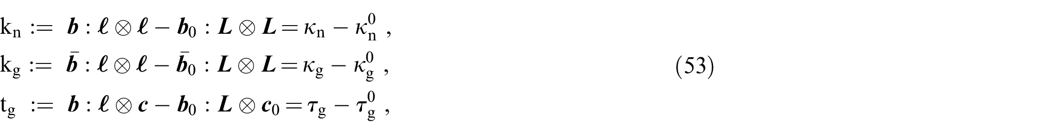
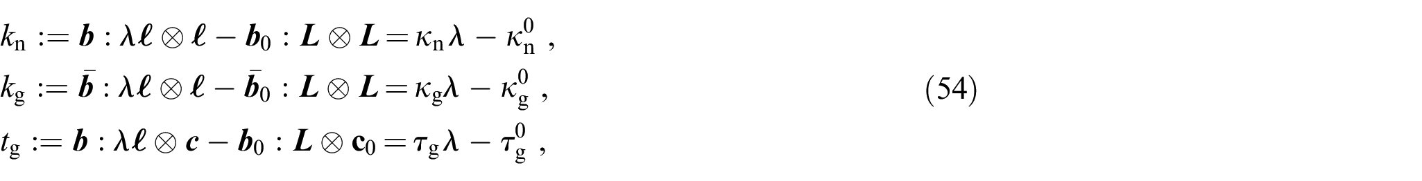
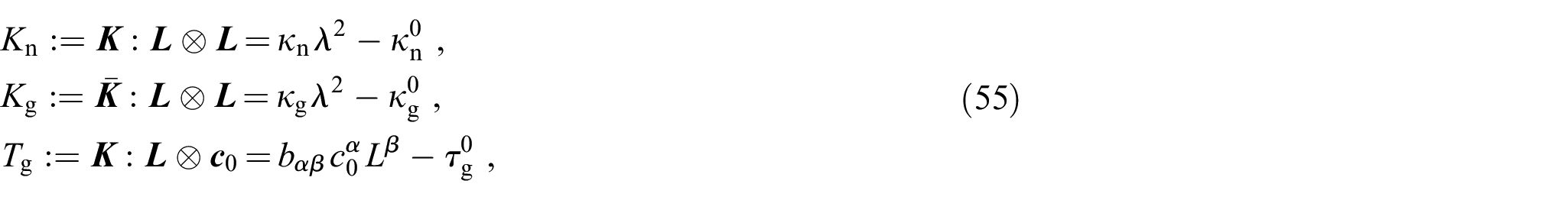
Remark 2.5. To measure the change in the curvatures, one can use the invariants

$$\begin{array}{c}{\mathrm{k}}_{\mathrm{n}}:=\mathit{b}:\mathit{\ell }\otimes \mathit{\ell }-{\mathit{b}}_0:\mathit{L}\otimes \mathit{L}={\kappa }_{\mathrm{n}}-{\kappa }_{\mathrm{n}}^0,\hfill \\ {\mathrm{k}}_{\mathrm{g}}:=\overline{\mathit{b}}:\mathit{\ell }\otimes \mathit{\ell }-{\overline{\mathit{b}}}_0:\mathit{L}\otimes \mathit{L}={\kappa }_{\mathrm{g}}-{\kappa }_{\mathrm{g}}^0,\hfill \\ {\mathrm{t}}_{\mathrm{g}}:=\mathit{b}:\mathit{\ell }\otimes \mathit{c}-{\mathit{b}}_0:\mathit{L}\otimes {\mathit{c}}_0={\tau }_{\mathrm{g}}-{\tau }_{\mathrm{g}}^0,\hfill \end{array}$$

(53)

called the absolute change in the normal curvature, geodesic curvature, and geodesic torsion, respectively. Here, ${•}^0$ denotes the corresponding quantities in the initial configuration.

Remark 2.6. However, the curvature changes (equation (53)) are not ideal for constitutive models, as they can lead to unphysical stress couples that respond to fiber stretching even when there is no bending. An example is pure dilatation, for example, due to thermal expansion or hydrostatic stress states as is discussed in example 7.4. To exclude fiber stretching, we define the invariants

$$\begin{array}{c}{k}_{\mathrm{n}}:=\mathit{b}:\lambda \mathit{\ell }\otimes \mathit{\ell }-{\mathit{b}}_0:\mathit{L}\otimes \mathit{L}={\kappa }_{\mathrm{n}}\lambda -{\kappa }_{\mathrm{n}}^0,\hfill \\ k_{\mathrm{g}}:=\overline{\mathit{b}}:\lambda \mathit{\ell }\otimes \mathit{\ell }-{\overline{\mathit{b}}}_0:\mathit{L}\otimes \mathit{L}={\kappa }_{\mathrm{g}}\lambda -{\kappa }_{\mathrm{g}}^0,\hfill \\ t_{\mathrm{g}}:=\mathit{b}:\lambda \mathit{\ell }\otimes \mathit{c}-{\mathit{b}}_0:\mathit{L}\otimes c_0={\tau }_{\mathrm{g}}\lambda -{\tau }_{\mathrm{g}}^0,\hfill \end{array}$$

(54)

called the stretch-excluded change in the normal curvature, geodesic curvature, and geodesic torsion, respectively.

Remark 2.7. Both curvature changes (53) and (54) can cause fiber tension apart from fiber bending. Therefore, one can use the so-called nominal change in the normal curvature, geodesic curvature, and geodesic torsion, defined by

$$\begin{array}{c}{K}_{\mathrm{n}}:=\mathit{K}:\mathit{L}\otimes \mathit{L}={\kappa }_{\mathrm{n}}{\lambda }^2-{\kappa }_{\mathrm{n}}^0,\hfill \\ K_{\mathrm{g}}:=\overline{\mathit{K}}:\mathit{L}\otimes \mathit{L}={\kappa }_{\mathrm{g}}{\lambda }^2-{\kappa }_{\mathrm{g}}^0,\hfill \\ T_{\mathrm{g}}:=\mathit{K}:\mathit{L}\otimes {\mathit{c}}_0=b_{\alpha \beta }{c}_0^{\alpha }{L}^{\beta }-{\tau }_{\mathrm{g}}^0,\hfill \end{array}$$

(55)

where $\mathit{K}$ and $\overline{\mathit{K}}$ are defined by equations (47) and (48), respectively. These invariants can also be found, for example, in the works by Steigmann and Dell’Isola [1] and Schulte et al. [36]. Since the measures (equation (55)) do not cause an axial tension in the fibers, their material tangents simplify significantly. Note however that, like equation (53), they can cause unphysical stress couples responding to fiber stretching.

Remark 2.8. The mentioned curvature measures (equations (53), (54), and (55)) are also listed in Table 1. It should be noted that all these measures are equivalent for inextensible fibers, that is, $\lambda =1$ , which is usually assumed for textile composites.

3. Balance laws

In this section, we discuss the balance laws for fibrous thin shells taking into account not only in-plane stretching and out-of-plane bending, but also in-plane bending. Like in classical Kirchhoff–Love shell theory, we directly postulate linear and angular momentum balance for our generalized Kirchhoff–Love shell with in-plane bending. Although the presented theory is not derived from general Cosserat theory, we show in Appendix 4 that our set of balance equations is consistent with that of Cosserat shell theory.

We consider that the out-of-plane shear energy and the out-of-plane thickness strain energy are negligible. The first condition amounts to the Kirchhoff–Love kinematical assumption of zero out-of-plane shear strains. The second condition is satisfied here by the plane stress assumption (i.e. zero thickness stress), which is commonly used for thin shells. It still allows for thickness changes, for example, due to large membrane stretching. Note, however, that these assumptions on the shear strains and thickness stress are mathematically independent of the thickness, so that the governing equations can be written directly in surface form without the need of a thickness variable. Instead, the influence of the thickness appears in the constitutive equations [2,5,10,11].

In the following, we first discuss in detail the theory with one embedded fiber family $\mathcal{C}$ . The extension to multiple fiber families is straightforward and will be discussed subsequently.

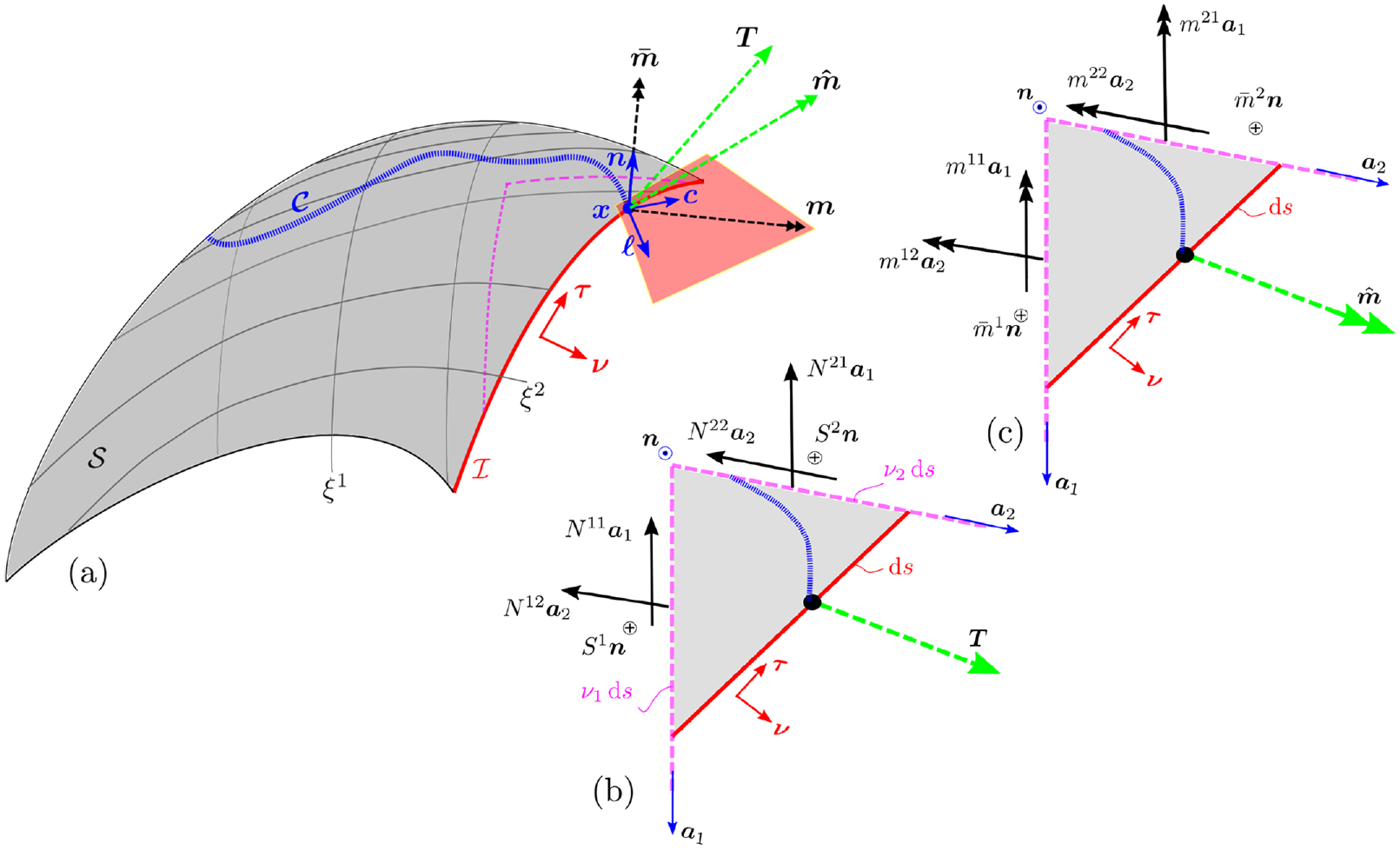
In order to define internal stresses and internal moment tensors, the shell $\mathcal{S}$ is virtually cut into two parts at position $\mathit{x}$ as depicted in Figure 2. On the parametrized cut, denoted by $\mathcal{I}(s)$ , we define the unit tangent vector $\mathit{\tau }:=\partial \mathit{x}/\partial s$ and the unit normal $\mathit{\nu }:=\mathit{\tau }\times \mathit{n}={\nu }_{\alpha }{\mathit{a}}^{\alpha }$ at $\mathit{x}$ .

Figure 2.

Internal stresses and moments: (a) illustration of physical traction vector $\mathit{T}$ and moment vector $\hat{\mathit{m}}$ acting on the cut $\mathcal{I}$ (red curve) through surface $\mathcal{S}$ with its embedded fiber $\mathcal{C}$ (blue curve). Both $\mathit{T}$ and $\hat{\mathit{m}}$ are general vectors in 3D space. The moment vector $\hat{\mathit{m}}$ can be decomposed into the component $\overline{\mathit{m}}$ , causing in-plane bending, and the component $\mathit{m}$ , causing out-of-plane bending and twisting. Vectors $\mathit{\ell }$ , $c$ , $\mathit{\nu }$ , $\mathit{\tau }$ , and $\mathit{m}$ lie in the tangent plane of $\mathcal{S}$ . (b) Stress and (c) moment components appearing on a triangular element—which is in force and moment equilibrium—under the action of the traction $\mathit{T}$ and moment $\hat{\mathit{m}}$ , respectively. These stress and moment components appear on the cuts that intersect with the tangent plane (pink dash lines). Assuming plane stress conditions, the stress and moment on any cut perpendicular to the surface normal $\mathit{n}$ (gray area) are neglected for the equilibrium of the triangular element.

3.1. Stress tensor

This section discusses Cauchy stress tensor $\mathbf{\sigma }$ for thin shells under plane-stress conditions. The influence of angular momentum balance on the stress tensor is then discussed in section 3.4.

The traction vector $\mathit{T}$ appearing on the cut can have arbitrary direction (see Figure 2(b)), but we can generally express it with respect to the basis $\{{\mathit{a}}_1,{\mathit{a}}_2,\mathit{n}\}$ as

$$\begin{array}{c}\mathit{T}=T^{\alpha }{\mathit{a}}_{\alpha }+T^3\mathit{n},\hfill \end{array}$$

(56)

where $T^{\alpha }$ and $T^3$ are the contravariant components of $\mathit{T}$ . This traction induces the Cauchy stress tensor $\mathbf{\sigma }$ . Following Cauchy’s theorem, the components of $\mathbf{\sigma }$ are balanced by the traction $\mathit{T}$ on an infinitesimal triangular element, as shown in Figure 2(b). Under plane-stress conditions, all stresses on any cut perpendicular to surface normal $\mathit{n}$ are neglected for the (force) equilibrium of the triangular element. That is, the components of tensor $\mathbf{\sigma }$ associated with bases $\mathit{n}\otimes {\mathit{a}}_{\alpha }$ and $\mathit{n}\otimes \mathit{n}$ are considered to be zero. This results in the asymmetry of tensor $\mathbf{\sigma }$ in the form,

$$\begin{array}{c}\mathbf{\sigma }=N^{\alpha \beta }{\mathit{a}}_{\alpha }\otimes {\mathit{a}}_{\beta }+S^{\alpha }{\mathit{a}}_{\alpha }\otimes \mathit{n},\hfill \end{array}$$

(57)

where $N^{\alpha \beta }$ and $S^{\alpha }$ are the membrane stress and out-of-plane shear stress components of $\mathbf{\sigma }$ . Accordingly, the components of $\mathbf{\sigma }$ on the cross-section perpendicular to ${\mathit{a}}^{\alpha }$ are defined by

$$\begin{array}{c}{\mathit{T}}^{\alpha }:={\mathbf{\sigma }}^{\mathrm{T}}{\mathit{a}}^{\alpha }=N^{\alpha \beta }{\mathit{a}}_{\beta }+S^{\alpha }\mathit{n},\hfill \end{array}$$

(58)

which is illustrated in Figure 2(b) for an infinitesimal triangular element on $\mathcal{S}$ . With this, we can write

$$\begin{array}{c}\mathbf{\sigma }={\mathit{a}}_{\alpha }\otimes {\mathit{T}}^{\alpha }.\hfill \end{array}$$

(59)

Furthermore, the force equilibrium of the triangle (see Figure 2(b)) gives

$$\begin{array}{c}\mathit{T}\mathrm{d}s=({\nu }_{\alpha }{N}^{\alpha \beta }){\mathit{a}}_{\beta }\mathrm{d}s+({\nu }_{\alpha }{S}^{\alpha })\mathit{n}\mathrm{d}s={\mathit{T}}^{\alpha }{\nu }_{\alpha }\mathrm{d}s,\hfill \end{array}$$

(60)

which implies Cauchy’s formula

$$\begin{array}{c}\mathit{T}=({\mathit{T}}^{\alpha }\otimes {\mathit{a}}_{\alpha })\mathit{\nu }={\mathbf{\sigma }}^{\mathrm{T}}\mathit{\nu },\hfill \end{array}$$

(61)

since ${\nu }_{\alpha }=\mathit{\nu }·{\mathit{a}}_{\alpha }$ . By comparing equation (61) with equation (56), we can further write

$$T^{\alpha }={\nu }_{\beta }{N}^{\beta \alpha },T^3={\nu }_{\alpha }{S}^{\alpha }.$$

(62)

Remark 3.1. Due to the presence of transverse shear components $S^{\alpha }$ , the traction vector $\mathit{T}$ has both in-plane and out-of-plane components as is seen from equation (56) and (62). As shown in section 3.4, in general, $N^{\alpha \beta }$ in equation (57) is not symmetric according to angular momentum balance. Instead, the so-called effective stress—denoted by ${\tilde{\sigma }}^{\alpha \beta }$ and defined in equation (93)—is symmetric according to angular momentum balance.

Remark 3.2. The format of the Cauchy stress (57) also contains all the stresses within a cut fiber. Indeed, consider a fiber $\mathcal{C}$ described by beam theory. According to beam theory, all stresses are neglected on a cut parallel to the fiber. Accordingly, the stress tensor in the fiber $\mathcal{C}$ —denoted by ${\mathbf{\sigma }}_{\mathrm{fib}}$ —can be written as

$${\mathbf{\sigma }}_{\mathrm{fib}}=\sigma \mathit{\ell }\otimes \mathit{\ell }+s_c\mathit{\ell }\otimes \mathit{c}+s_{\mathrm{n}}\mathit{\ell }\otimes \mathit{n},$$

(63)

where $\sigma$ , $s_c$ , and $s_{\mathrm{n}}$ denote the axial stress and the two shear stresses. By inserting the basis vectors $\mathit{\ell }={\mathit{\ell }}^{\alpha }{\mathit{a}}_{\alpha }$ , and $\mathit{c}=c^{\alpha }{\mathit{a}}_{\alpha }$ , equation (63) becomes

$${\mathbf{\sigma }}_{\mathrm{fib}}=N^{\alpha \beta }{\mathit{a}}_{\alpha }\otimes {\mathit{a}}_{\beta }+S^{\alpha }{\mathit{a}}_{\alpha }\otimes \mathit{n},$$

(64)

with

$$\begin{array}{c}{N}^{\alpha \beta }=\sigma {\ell }^{\alpha \beta }+s_c{\ell }^{\alpha }{c}^{\beta },\hfill \\ \multicolumn{1}{c}{S^{\alpha }=s_{\mathrm{n}}{\ell }^{\alpha }.}\end{array}$$

(65)

3.2. Generalized moment tensor

This section discusses the moment tensor $\widehat{\mathit{\mu }}$ for Kirchhoff–Love shells with in-plane bending. Also, equivalent stress couple tensors $\mathit{\mu }$ and $\overline{\mathit{\mu }}$ are defined by introducing stress couple vectors that are equivalent to the in-plane and out-of-plane bending moments.

At position $\mathit{x}$ on cut $\mathcal{I}(s)$ (see Figure 2(c)), the bending moment vector, denoted by $\hat{\mathit{m}}$ (with unit moment per unit length), is allowed to have both in-plane and out-of-plane components. It can be expressed with respect to basis $\{\mathit{\tau },\mathit{\nu },\mathit{n}\}$ as

$$\hat{\mathit{m}}:=m_{\mathit{\tau }}\mathit{\tau }+m_{\nu }\mathit{\nu }+\overline{m}\mathit{n},$$

(66)

where ⁷ $\overline{m}\mathit{n}=:\overline{\mathit{m}}$ is the moment causing in-plane bending and

$$m_{\tau }\mathit{\tau }+m_{\nu }\mathit{\nu }=:\mathit{m},$$

(67)

denotes the combined moment causing out-of-plane bending and twisting.

Similar to the Cauchy stress tensor (equation (57)), all moments on a cut perpendicular to surface normal $\mathit{n}$ are zero under Kirchhoff–Love assumptions. The total moment tensor $\hat{\mu }$ induced by $\hat{\mathit{m}}$ can thus be expressed in the form

$$\begin{array}{c}\hat{\mathit{\mu }}:=m^{\alpha \beta }{\mathit{a}}_{\alpha }\otimes {\mathit{a}}_{\beta }+{\overline{m}}^{\alpha }{\mathit{a}}_{\alpha }\otimes \mathit{n}.\hfill \end{array}$$

(68)

In this form, the first term $m^{\alpha \beta }{\mathit{a}}_{\alpha }\otimes {\mathit{a}}_{\beta }$ combines both out-of-plane bending and twisting in response to a change in the out-of-plane curvature of $\mathcal{S}$ , while the second term ${\overline{m}}^{\alpha }{\mathit{a}}_{\alpha }\otimes \mathit{n}$ is the response to a change in the in-plane curvature of fiber $\mathcal{C}$ .

The components of ${\hat{\mathit{\mu }}}^{\mathrm{T}}$ , on the cross-section perpendicular to ${\mathit{a}}^{\alpha }$ , thus read as (see Figure 2(c))

$$\begin{array}{c}{\hat{\mathit{m}}}^{\alpha }:={\hat{\mathit{\mu }}}^{\mathrm{T}}{\mathit{a}}^{\alpha }=m^{\alpha \beta }{\mathit{a}}_{\beta }+{\overline{m}}^{\alpha }\mathit{n}.\hfill \end{array}$$

(69)

Here, moment vectors $m^{\alpha \beta }{\mathit{a}}_{\beta }$ and ${\overline{m}}^{\alpha }\mathit{n}$ are associated with the angular velocity vector around the in-plane axis

$$\mathit{n}\times \stackrel{·}{\mathit{n}}=(\mathit{n}·{\stackrel{·}{\mathit{a}}}^{\alpha }){\mathit{a}}_{\alpha }\times \mathit{n},$$

(70)

and the out-of-plane axis $\mathit{n}=\mathit{\ell }\times \mathit{c}={\mathit{\ell }}^{\alpha }{\mathit{a}}_{\alpha }\times \mathit{c}$ , respectively. Therefore, it is mathematically convenient to express ${\hat{\mathit{m}}}^{\alpha }$ with respect to the basis $\{{\mathit{a}}_1\times \mathit{n},{\mathit{a}}_2\times \mathit{n},\mathit{n}\}$ , that is,

$$\begin{array}{c}{\hat{\mathit{m}}}^{\alpha }=M^{\alpha \beta }({\mathit{a}}_{\beta }\times \mathit{n})+{\overline{M}}^{\alpha \beta }({\mathit{a}}_{\beta }\times \mathit{c})\hfill \\ \multicolumn{1}{c}{=\mathit{n}\times {\mathit{M}}^{\alpha }+\mathit{c}\times {\overline{\mathit{M}}}^{\alpha },}\end{array}$$

(71)

where $M^{\alpha \beta }$ and ${\overline{M}}^{\alpha \beta }$ denote the components of vectors ${\hat{\mathit{m}}}^{\alpha }$ in directions ${\mathit{a}}_{\beta }\times \mathit{n}$ and ${\mathit{a}}_{\beta }\times \mathit{c}$ , respectively. Here, we have defined the so-called stress couple vectors for out-of-plane and in-plane bending ⁸

$${\mathit{M}}^{\alpha }:=-M^{\alpha \beta }{\mathit{a}}_{\beta },\mathrm{and}{\overline{\mathit{M}}}^{\alpha }:=-{\overline{M}}^{\alpha \beta }{\mathit{a}}_{\beta },\mathrm{with}{\overline{M}}^{\alpha \beta }:={\overline{m}}^{\alpha }{\ell }^{\beta }.$$

(72)

Equation (68) thus becomes

$$\begin{array}{c}\hat{\mu }:=M^{\alpha \beta }{\mathit{a}}_{\alpha }\otimes ({\mathit{a}}_{\beta }\times \mathit{n})+{\overline{M}}^{\alpha \beta }{\mathit{a}}_{\alpha }\otimes ({\mathit{a}}_{\beta }\times \mathit{c}).\hfill \end{array}$$

(73)

Similar to equation (61), moment equilibrium of the triangle (see Figure 2(c)) results in Cauchy’s formula

$$\hat{\mathit{m}}={\hat{\mathit{m}}}^{\alpha }{\nu }_{\alpha }=\mathit{n}\times \mathit{M}+\mathit{c}\times \overline{\mathit{M}}={\hat{\mathit{\mu }}}^{\mathrm{T}}\mathit{\nu },$$

(74)

where

$$\mathit{M}:={\mathit{M}}^{\alpha }{\nu }_{\alpha },\mathrm{and}\overline{\mathit{M}}:={\overline{\mathit{M}}}^{\alpha }{\nu }_{\alpha }$$

(75)

are referred to as the stress couple vectors associated with out-of-plane and in-plane bending, respectively. By comparing equations (74) and (66), the stress couple vectors $\mathit{M}$ and $\overline{\mathit{M}}$ can be related to their moment vector counterparts by

$$\mathit{m}=\mathit{n}\times \mathit{M},\mathrm{and}\overline{\mathit{m}}=\mathit{c}\times \overline{\mathit{M}},\mathrm{with}\overline{\mathit{M}}=-\overline{m}\ell .$$

(76)

In line with previous works, see, for example, Sauer and Duong [10], we can also define the stress couple tensors, ⁸

$$\mathit{\mu }:=-M^{\alpha \beta }{\mathit{a}}_{\alpha }\otimes {\mathit{a}}_{\beta },\mathrm{and}\overline{\mathit{\mu }}:=-{\overline{M}}^{\alpha \beta }{\mathit{a}}_{\alpha }\otimes {\mathit{a}}_{\beta },$$

(77)

associated with out-of-plane and in-plane bending, respectively. In view of eqution (74), we obtain the mapping

$$\mathit{M}={\mathit{\mu }}^{\mathrm{T}}\mathit{\nu },\mathrm{and}\overline{\mathit{M}}={\overline{\mathit{\mu }}}^{\mathrm{T}}\mathit{\nu }.$$

(78)

In order to relate the components of the moment vector (equation (66)) to the components of the stress couple tensors, we can equate equations (66) and (74). This results in

$$\begin{array}{c}{m}_{\nu }:=\hat{\mathit{m}}·\mathit{\nu }=\mathit{m}·\mathit{\nu }=M^{\alpha \beta }{\nu }_{\alpha }{\tau }_{\beta },\hfill \\ \multicolumn{1}{c}{m_{\tau }:=\hat{\mathit{m}}·\mathit{\tau }=\mathit{m}·\mathit{\tau }=-M^{\alpha \beta }{\nu }_{\alpha }{\nu }_{\beta },}\\ \multicolumn{1}{c}{\overline{m}:=\hat{\mathit{m}}·\mathit{n}=\overline{\mathit{m}}·\mathit{n}={\overline{M}}^{\alpha \beta }{\nu }_{\alpha }{\ell }_{\beta }={\overline{m}}^{\alpha }{\nu }_{\alpha },}\end{array}$$

(79)

where we have used the relations ${\mathit{a}}_{\beta }\times \mathit{n}={\tau }_{\beta }\mathit{\nu }-{\nu }_{\beta }\mathit{\tau }$ due to ${\mathit{a}}_{\alpha }={\tau }_{\alpha }\mathit{\tau }+{\nu }_{\alpha }\mathit{\nu }$ .

Remark 3.3. Similar to equation (63), the moment tensor for a fiber described by beam theory—denoted by ${\hat{\mathit{\mu }}}_{\mathrm{fib}}$ —can also be written in the form of equation (68), that is,

$${\hat{\mathit{\mu }}}_{\mathrm{fib}}:={\mu }_{\ell }\mathit{\ell }\otimes \mathit{\ell }+{\mathit{\mu }}_c\mathit{\ell }\otimes \mathit{c}+\overline{\mathit{\mu }}\mathit{\ell }\otimes \mathit{n}=m^{\alpha \beta }{\mathit{a}}_{\alpha }\otimes {\mathit{a}}_{\beta }+{\overline{m}}^{\alpha }{\mathit{a}}_{\alpha }\otimes \mathit{n}.$$

(80)

Here, ${\mu }_{\ell }$ , ${\mu }_c$ , and $\overline{\mu }$ denote twisting, out-of-plane bending, and in-plane bending moments in fiber $\mathcal{C}$ , respectively, and we have identified

$$\begin{array}{c}{m}^{\alpha \beta }={\mu }_{\ell }{\ell }^{\alpha \beta }+{\mu }_c{\ell }^{\alpha }{c}^{\beta },\hfill \\ \multicolumn{1}{c}{{\overline{m}}^{\alpha }=\overline{\mu }{\ell }^{\alpha }.}\end{array}$$

(81)

Remark 3.4. Furthermore, inserting ${\overline{m}}^{\alpha }$ from equation (81) into equations (72.3) and (79.3) gives

$$\begin{array}{c}{\overline{M}}^{\alpha \beta }=\overline{\mu }{\ell }^{\alpha \beta }\hfill \\ \multicolumn{1}{c}{\overline{m}=\overline{\mu }\mathit{\ell }·\mathit{\nu }.}\end{array}$$

(82)

Therefore, we can conclude that ${\overline{M}}^{\alpha \beta }$ is symmetric. Note that $\overline{\mu }$ does not depend on the cut $\mathcal{I}$ since it is a component of the internal moment tensor, but $\overline{m}$ does depend on $\mathcal{I}$ as seen in equation (82.2). For example, $\overline{m}=0$ when the cut is parallel to the fiber, that is, when $\mathit{\ell }·\mathit{\nu }=0$ .

3.3. Balance of linear momentum

Consider body forces $\mathit{f}$ acting on an arbitrary simply-connected region $\mathcal{R}\subset \mathcal{S}$ . The balance of linear momentum implies that the temporal change of linear momentum is equal to the resultant of all acting external forces. That is,

$$\frac{D}{\mathrm{Dt}}{\int }_{\mathcal{R}}\rho \mathit{\upsilon }\mathrm{d}a={\int }_{\mathcal{R}}\mathit{f}\mathrm{d}a+{\int }_{\partial \mathcal{R}}\mathit{T}\mathrm{d}s,\forall \in \mathcal{S},$$

(83)

where $\mathit{\upsilon }$ denotes the material velocity of the surface. Inserting $\mathit{T}$ from equation (61), and applying the surface divergence theorem and conservation of mass, one obtains the local form of linear momentum balance

$$\begin{array}{c}\mathrm{di}{\mathrm{v}}_{\mathrm{s}}{\mathbf{\sigma }}^{\mathrm{T}}+\mathit{f}=\rho \stackrel{·}{\mathit{\upsilon }},\hfill \end{array}$$

(84)

where $\mathrm{di}{\mathrm{v}}_{\mathrm{s}}$ denotes the surface divergence operator, defined by $\mathrm{di}{\mathrm{v}}_{\mathrm{s}}•:={•}_{,\alpha }·{\mathit{a}}^{\alpha }.$ Note that equation (84) can also be written in the form [10]

$$\begin{array}{c}{\mathit{T}}_{;\alpha }^{\alpha }+\mathit{f}=\rho \stackrel{·}{\mathit{\upsilon }},\hfill \end{array}$$

(85)

since

$$\mathrm{di}{\mathrm{v}}_{\mathrm{s}}{\mathbf{\sigma }}^{\mathrm{T}}={\mathbf{\sigma }}_{,\beta }^{\mathrm{T}}·{\mathit{a}}^{\beta }={\mathit{T}}_{,\alpha }^{\alpha }+{\mathrm{\Gamma }}_{\alpha \beta }^{\beta }{\mathit{T}}^{\alpha }={\mathit{T}}_{;\alpha }^{\alpha },$$

(86)

follows from equation (59).

3.4. Balance of angular momentum

The balance of angular momentum implies that the temporal change of angular momentum is equal to the resultant of all external moments. That is,

$$\frac{D}{\mathrm{Dt}}{\int }_{\mathcal{R}}\rho \mathit{x}\times \mathit{\upsilon }\mathrm{d}a={\int }_{\mathcal{R}}\mathit{x}\times \mathit{f}\mathrm{d}a+{\int }_{\partial \mathcal{R}}\mathit{x}\times \mathit{T}\mathrm{d}s+{\int }_{\partial \mathcal{R}}\hat{\mathit{m}}\mathrm{d}s,$$

(87)

where $\hat{\mathit{m}}$ includes both in-plane and out-of-plane bending moments acting on $\partial \mathcal{R}$ . From equations (61) and (74), the surface divergence theorem gives

$${\int }_{\partial \mathcal{R}}\mathit{x}\times \mathit{T}\mathrm{d}s={\int }_{\mathcal{R}}({\mathit{a}}_{\alpha }\times {\mathit{T}}^{\alpha }+\mathit{x}\times \mathrm{di}{\mathrm{v}}_{\mathrm{s}}{\mathbf{\sigma }}^{\mathrm{T}})\mathrm{d}a$$

(88)

and

$${\int }_{\partial \mathcal{R}}\hat{\mathit{m}}\mathrm{d}s={\int }_{\mathcal{R}}\mathrm{di}{\mathrm{v}}_{\mathrm{s}}{\hat{\mathit{\mu }}}^{\mathrm{T}}\mathrm{d}a.$$

(89)

Inserting these equations into equation (87) and applying local mass conservation gives

$${\int }_{\mathcal{R}}({\mathit{a}}_{\alpha }\times {\mathit{T}}^{\alpha }+\mathrm{di}{\mathrm{v}}_{\mathrm{s}}{\hat{\mathit{\mu }}}^{\mathrm{T}})\mathrm{d}a+{\int }_{\mathcal{R}}\mathit{x}\times (\mathrm{di}{\mathrm{v}}_{\mathrm{s}}{\sigma }^{\mathrm{T}}+\mathit{f}-\rho \stackrel{·}{\mathit{\upsilon }})\mathrm{d}a=0.$$

(90)

The second integral in equation (90) vanishes due to equation (84). This leads to the local form of the angular momentum balance,

$$\begin{array}{c}{\mathit{a}}_{\alpha }\times {\mathit{T}}^{\alpha }+\mathrm{di}{\mathrm{v}}_{\mathrm{s}}{\hat{\mathit{\mu }}}^{\mathrm{T}}=0.\hfill \end{array}$$

(91)

Keeping equation (82.1) in mind, the surface divergence of tensor ${\hat{\mathit{\mu }}}^{\mathrm{T}}$ follows from equation (73) as

$$\begin{array}{c}\mathrm{di}{\mathrm{v}}_{\mathrm{s}}{\hat{\mathit{\mu }}}^{\mathrm{T}}=(-M^{\alpha \beta }{b}_{\alpha }^{\gamma }+{\overline{m}}_{;\alpha }^{\alpha }{\ell }^{\beta }{c}^{\gamma }){\mathit{a}}_{\beta }\times {\mathit{a}}_{\gamma }+(M_{;\beta }^{\beta \alpha }+\overline{\mu }{\tau }_{\mathrm{g}}{\ell }^{\alpha }-\overline{\mu }{\kappa }_{\mathrm{n}}{c}^{\alpha }){\mathit{a}}_{\alpha }\times \mathit{n},\hfill \end{array}$$

(92)

where we have used ${\mathit{a}}_{\alpha }={\ell }_{\alpha }\mathit{\ell }+c_{\alpha }\mathit{c}=({\mathit{\ell }}_{\alpha }{c}^{\gamma }-c_{\alpha }{\mathit{\ell }}^{\gamma }){\mathit{a}}_{\gamma }\times \mathit{n}$ . Inserting equations (92) and (58) into equation (91) then implies that the so-called effective membrane stress ⁹

$$\begin{array}{c}{\tilde{\sigma }}^{\alpha \beta }:=N^{\alpha \beta }-M^{\gamma \alpha }{b}_{\gamma }^{\beta }+{\overline{m}}_{;\gamma }^{\gamma }{\ell }^{\alpha }{c}^{\beta }\hfill \end{array}$$

(93)

is symmetric, and that the shear stress is given by

$$\begin{array}{c}{S}^{\alpha }=-M_{;\beta }^{\beta \alpha }+\overline{\mu }({\kappa }_{\mathrm{n}}{c}^{\alpha }-{\tau }_{\mathrm{g}}{\ell }^{\alpha }).\hfill \end{array}$$

(94)

Thus, angular momentum balance implies the symmetry of the effective stress ${\tilde{\sigma }}^{\alpha \beta }$ instead of the Cauchy stress $N^{\alpha \beta }$ . The latter is only symmetric when there is no in-plane and out-of-plane bending resistance.

Remark 3.5. The last term in stress expression (93) relates to the in-plane shear force in the fiber, which, in accordance with the assumed Euler-Bernoulli kinematics, follows as the derivative of the in-plane bending moment.

3.5. Mechanical power balance

The mechanical power balance can be obtained from local momentum balance (eqation (84)). To this end, we can write

$${\int }_{\mathcal{R}}\mathit{\upsilon }·(\mathrm{di}{\mathrm{v}}_{\mathrm{s}}{\mathbf{\sigma }}^{\mathrm{T}}+\mathit{f}-\rho \stackrel{·}{\mathit{\upsilon }})\mathrm{d}a=0.$$

(95)

Here, the divergence term can be transformed by the identity

$$\begin{array}{c}\mathit{\upsilon }·\mathrm{di}{\mathrm{v}}_{\mathrm{s}}{\mathbf{\sigma }}^{\mathrm{T}}=\mathrm{di}{\mathrm{v}}_{\mathrm{s}}(\mathit{\upsilon }{\mathbf{\sigma }}^{\mathrm{T}})-{\mathbf{\sigma }}^{\mathrm{T}}:{\nabla }_{\mathrm{s}}\mathit{\upsilon },\hfill \end{array}$$

(96)

by the divergence theorem

$${\int }_{\mathcal{R}}\mathrm{di}{\mathrm{v}}_{\mathrm{s}}(\mathit{\upsilon }{\mathbf{\sigma }}^{\mathrm{T}})\mathrm{d}a={\int }_{\partial \mathcal{R}}\mathit{\upsilon }·{\mathbf{\sigma }}^{\mathrm{T}}\mathit{\nu }\mathrm{d}s={\int }_{\partial \mathcal{R}}\mathit{\upsilon }·\mathit{T}\mathrm{d}s,$$

(97)

and using the relation

$${\mathbf{\sigma }}^{\mathrm{T}}:{\nabla }_{\mathrm{s}}\mathit{\upsilon }=N^{\alpha \beta }{\mathit{a}}_{\beta }·{\stackrel{·}{\mathit{a}}}_{\alpha }+S^{\alpha }\mathit{n}·{\stackrel{·}{\mathit{a}}}_{\alpha }.$$

(98)

Inserting equations (93) and (94) into equation (98) gives

$${\mathbf{\sigma }}^{\mathrm{T}}:{\nabla }_{\mathrm{s}}\mathit{\upsilon }=\frac{1}{2}{\tilde{\sigma }}^{\alpha \beta }{\stackrel{·}{a}}_{\alpha \beta }-M^{\alpha \beta }{\mathit{n}}_{;\alpha }·{\stackrel{·}{\mathit{a}}}_{\beta }-\overline{\mu }({\kappa }_{\mathrm{n}}\mathit{c}·\stackrel{·}{\mathit{n}}-{\tau }_{\mathrm{g}}\mathit{\ell }·\stackrel{·}{\mathit{n}})-M_{;\beta }^{\beta \alpha }\mathit{n}·{\stackrel{·}{\mathit{a}}}_{\alpha }+{\overline{m}}_{;\alpha }^{\alpha }\mathit{\ell }·\stackrel{·}{c}.$$

(99)

Considering equations (15.2), (36), and (81.2), the last two terms can be written as

$$\begin{array}{c}{M}_{;\beta }^{\beta \alpha }\mathit{n}·{\stackrel{·}{\mathit{a}}}_{\alpha }={(\stackrel{·}{\mathit{n}}·{\mathit{M}}^{\alpha })}_{;\alpha }+M^{\alpha \beta }{\stackrel{·}{\mathit{n}}}_{;\alpha }·{\mathit{a}}_{\beta },\hfill \\ \multicolumn{1}{c}{{\overline{m}}_{;\alpha }^{\alpha }\mathit{\ell }·\stackrel{·}{\mathit{c}}={({\overline{m}}^{\alpha }\mathit{\ell }·\stackrel{·}{\mathit{c}})}_{;\alpha }+{\overline{m}}^{\alpha }\stackrel{·}{\overline{\left(c^{\beta }{\ell }_{\beta ;\alpha }\right)}}+\overline{\mu }({\kappa }_{\mathrm{n}}\mathit{c}·\stackrel{·}{\mathit{n}}-{\tau }_{\mathrm{g}}\mathit{\ell }·\stackrel{·}{\mathit{n}}).}\end{array}$$

(100)

By taking equations (96), (97), (99), (100) and local mass conservation into account, equation (95) becomes

$$\begin{array}{c}\stackrel{·}{K}+P_{\mathrm{int}}=P_{\mathrm{ext}},\hfill \end{array}$$

(101)

where

$$\stackrel{·}{K}={\int }_{\mathcal{R}}\rho \mathit{\upsilon }·\stackrel{·}{\mathit{\upsilon }}\mathrm{d}a$$

(102)

is the rate of kinetic energy,

$$P_{\mathrm{int}}=\frac{1}{2}{\int }_{\mathcal{R}}{\tilde{\sigma }}^{\alpha \beta }{\stackrel{·}{a}}_{\alpha \beta }\mathrm{d}a+{\int }_{\mathcal{R}}{M}^{\alpha \beta }{\stackrel{·}{b}}_{\alpha \beta }\mathrm{d}a+{\int }_{\mathcal{R}}{\overline{m}}^{\alpha }\stackrel{·}{\overline{\left(c^{\beta }{\ell }_{\beta ;\alpha }\right)}}\mathrm{d}a,$$

(103)

is the internal power, and

$$P_{\mathrm{ext}}={\int }_{\mathcal{R}}\mathit{\upsilon }·\mathit{f}\mathrm{d}a+{\int }_{\partial \mathcal{R}}\mathit{\upsilon }·\mathit{T}\mathrm{d}s+{\int }_{\partial \mathcal{R}}\stackrel{·}{\mathit{n}}·\mathit{M}\mathrm{d}s+{\int }_{\partial \mathcal{R}}\stackrel{·}{\mathit{c}}·\overline{\mathit{M}}\mathrm{d}s$$

(104)

denotes the external power. The last term in $P_{\mathrm{int}}$ can be written in alternative forms, as is discussed in the following section. The mechanical power balance (equation (101)) simplifies to the expression in Sauer and Duong [10] for ${\overline{m}}^{\alpha }\equiv 0$ and $\overline{M}=0$ .

4. Work-conjugate variables and constitutive equations

As seen from expression (103), the internal stress power per current area reads

$${\stackrel{·}{w}}_{\mathrm{int}}:=\frac{1}{2}{\tilde{\sigma }}^{\alpha \beta }{\stackrel{·}{a}}_{\alpha \beta }+M^{\alpha \beta }{\stackrel{·}{b}}_{\alpha \beta }+{\overline{m}}^{\alpha }\stackrel{·}{\overline{\left(c^{\beta }{\ell }_{\beta ;\alpha }\right)}},$$

(105)

which directly shows work-conjugate pairs. Accordingly, $c^{\beta }{\ell }_{\beta ;\alpha }{\mathit{A}}^{\alpha }=\mathit{c}{\overline{\nabla }}_{\mathrm{s}}\mathit{\ell }{\mathit{F}}^{-1}$ is a strain measure for the change in the in-plane curvatures. As shown in Appendix 3, the strain measure $c^{\beta }{\ell }_{\beta ;\alpha }$ is frame invariant under superimposed rigid body motion of the shell. However, it is somewhat unintuitive and thus inconvenient for the construction of material models. In the following, we will present two approaches with alternative definitions of this strain measure.

4.1. Geodesic curvature-based approach

This approach uses the geodesic curvature ${\kappa }_{\mathrm{g}}$ instead of $c^{\beta }{\ell }_{\beta ;\alpha }$ within the in-plane bending power. Namely, inserting ${\overline{m}}^{\alpha }$ from equation (81.2) into equation (105) and rearranging terms gives

$$\begin{array}{c}{\stackrel{·}{w}}_{\mathrm{int}}:=\frac{1}{2}{\sigma }^{\alpha \beta }{\stackrel{·}{a}}_{\alpha \beta }+M^{\alpha \beta }{\stackrel{·}{b}}_{\alpha \beta }+\overline{\mu }{\stackrel{·}{\kappa }}_{\mathrm{g}},\hfill \\ \mathrm{with}{\sigma }^{\alpha \beta }:={\tilde{\sigma }}^{\alpha \beta }+\overline{\mu }{\kappa }_{\mathrm{g}}{\ell }^{\alpha \beta }.\hfill \end{array}$$

(106)

Here, ${\sigma }^{\alpha \beta }$ represents the components of an effective membrane stress tensor. ¹⁰ It is symmetric as both ${\tilde{\sigma }}^{\alpha \beta }$ and ${\ell }^{\alpha \beta }$ are symmetric. The internal power (103) then becomes

$$P_{\mathrm{int}}=\frac{1}{2}{\int }_{{\mathcal{R}}_0}{\tau }^{\alpha \beta }{\stackrel{·}{a}}_{\alpha \beta }\mathrm{d}A+{\int }_{{\mathcal{R}}_0}{M}_0^{\alpha \beta }{\stackrel{·}{b}}_{\alpha \beta }\mathrm{d}A+{\int }_{{\mathcal{R}}_0}{\overline{\mu }}_0{\stackrel{·}{\kappa }}_{\mathrm{g}}\mathrm{d}A,$$

(107)

where ${\mathcal{R}}_0\in {\mathcal{S}}_0$ and

$${\tau }^{\alpha \beta }:=J{\sigma }^{\alpha \beta },M_0^{\alpha \beta }:=J{M}^{\alpha \beta },{\overline{\mu }}_0:=J\overline{\mu }.$$

(108)

These are the nominal quantities corresponding to the physical quantities ${\sigma }^{\alpha \beta }$ , $M^{\alpha \beta }$ , and $\overline{\mu }$ , respectively. Accordingly, we can assume a stored energy function of an hyperelastic shell in the form

$$\begin{array}{c}W=\stackrel{⌣}{W}(a_{\alpha \beta },b_{\alpha \beta },{\kappa }_{\mathrm{g}};h^{\alpha \beta }),\hfill \end{array}$$

(109)

where $h^{\alpha \beta }$ collectively represents the components of the structural tensor(s), for example, ${\ell }^{\alpha \beta }$ , $c^{\alpha \beta }$ , or, $c^{\alpha }{\ell }^{\beta }$ , that characterize material anisotropy due to embedded fibers. Equation (109) can equivalently be expressed in terms of invariants. All the strain measures $a_{\alpha \beta }$ , $b_{\alpha \beta }$ , ${\kappa }_{\mathrm{g}}$ , and $h^{\alpha \beta }$ used in equation (109) are frame invariant under superimposed rigid body motions as shown in Appendix 3. Using the usual arguments of Coleman and Noll [38], the constitutive equations can be written as

$${\tau }^{\alpha \beta }=2\frac{\partial \stackrel{⌣}{W}}{\partial a_{\alpha \beta }},M_0^{\alpha \beta }=\frac{\partial \stackrel{⌣}{W}}{\partial b_{\alpha \beta }},{\overline{\mu }}_0=\frac{\partial \stackrel{⌣}{W}}{\partial {\kappa }_{\mathrm{g}}}.$$

(110)

Remark 4.1. Compared to classical Kirchhoff–Love shell theory (see, for example, Naghdi [2] and Sauer and Duong [10]), the effective membrane stress ${\sigma }^{\alpha \beta }$ in equation (106.2) additionally contains the high-order bending term $\overline{\mu }$ and the in-plane fiber shear term $m_{;\gamma }^{\gamma }$ (see equation (93)). For slender fibers, they are negligible since the in-plane bending stiffness is usually much smaller than the membrane stiffness. However, these terms may become significant when there is a large (usually local) change in curvature (e.g. at shear bands).

Remark 4.2. Although a constitutive formulation following from equation (107) appears elegant, expression (110.3) is restricted to a material response expressible in terms of the geodesic curvature ${\kappa }_{\mathrm{g}}$ . Therefore, this setup might be unsuited for complex material behavior, for example, due to fiber dispersion [21]. In such cases, a more sophisticated structural tensor is usually desired for the in-plane bending response, and it thus may not always be possible to express $W$ in terms of ${\kappa }_{\mathrm{g}}$ . This motivates the following director gradient-based approach.

Remark 4.3. In equation (110), the stress components ${\tau }^{\alpha \beta }$ and $M_0^{\alpha \beta }$ , together with the strain components $a_{\alpha \beta }$ and $b_{\alpha \beta }$ in equation (109), are defined in the parameter space $\mathcal{P}$ , where they can be treated as independent variables without forming them into tensors. It is possible, though, to construct different stress and strain tensors from these components, such that their scalar product results in the same power as in equation (107). For example, ${\tau }^{\alpha \beta }$ can be the components of the Kirchhoff surface stress tensor $\hat{\mathit{\tau }}:={\tau }^{\alpha \beta }{\mathit{a}}_{\alpha }\otimes {\mathit{a}}_{\beta }$ , the second Piola–Kirchhoff stress tensor $\mathit{S}$ , or the first Piola–Kirchhoff stress tensor $\mathit{P}$ but with different bases. Indeed, $\mathit{S}={\mathit{F}}^{\mathrm{T}}\hat{\mathit{\tau }}\mathit{F}={\tau }^{\alpha \beta }{\mathit{A}}_{\alpha }\otimes {\mathit{A}}_{\beta }$ , and $\mathit{P}=\mathit{F}\mathit{S}={\tau }^{\alpha \beta }{\mathit{a}}_{\alpha }\otimes {\mathit{A}}_{\beta }$ . The strain variables work-conjugate to $\hat{\mathit{\tau }}$ , $\mathit{S}$ , and $\mathit{P}$ are related to the rate of surface deformation tensor $\mathit{D}$ , the Green–Lagrange surface strain tensor $\mathit{E}$ (or $\frac{1}{2}$ C ), and the surface deformation gradient tensor $\mathit{F}$ , respectively, since $\hat{\mathit{\tau }}:\mathit{D}=\mathit{S}:\stackrel{·}{\mathit{E}}=\mathit{S}:\frac{1}{2}\stackrel{·}{\mathit{C}}=\mathit{P}:\stackrel{·}{\mathit{F}}=\frac{1}{2}{\tau }^{\alpha \beta }{\stackrel{·}{a}}_{\alpha \beta }$ . See also Remark 4 in [39].

4.2. Director gradient-based approach

In this approach, the power expression (105) is rewritten by employing relation (38) and definitions (72.3) and (34) as

$${\stackrel{·}{w}}_{\mathrm{int}}:=\frac{1}{2}{\sigma }^{\alpha \beta }{\stackrel{·}{a}}_{\alpha \beta }+M^{\alpha \beta }{\stackrel{·}{b}}_{\alpha \beta }+{\overline{M}}^{\alpha \beta }{\stackrel{·}{\overline{b}}}_{\beta \alpha },$$

(111)

where ${\sigma }^{\alpha \beta }$ is now defined by ¹⁰

$$\begin{array}{c}{\sigma }^{\alpha \beta }:={\tilde{\sigma }}^{\alpha \beta }+({\overline{M}}^{\gamma \delta }{c}_{\delta ;\gamma }){\ell }^{\alpha \beta }.\hfill \end{array}$$

(112)

Thus, the internal power can be written as

$$P_{\mathrm{int}}=\frac{1}{2}{\int }_{{\mathcal{R}}_0}{\tau }^{\alpha \beta }{\stackrel{·}{a}}_{\alpha \beta }\mathrm{d}A+{\int }_{{\mathcal{R}}_0}{M}_0^{\alpha \beta }{\stackrel{·}{b}}_{\alpha \beta }\mathrm{d}A+{\int }_{{\mathcal{R}}_0}{\overline{M}}_0^{\alpha \beta }{\stackrel{·}{\overline{b}}}_{\alpha \beta }\mathrm{d}A,$$

(113)

where we have again used (108) and defined

$${\overline{M}}_0^{\alpha \beta }:=J{\overline{M}}^{\alpha \beta }.$$

(114)

Accordingly, the stored energy function can now be given in the form

$$\begin{array}{c}W=\hat{W}(a_{\alpha \beta },b_{\alpha \beta },{\overline{b}}_{\alpha \beta };h^{\alpha \beta }).\hfill \end{array}$$

(115)

This function can also be expressed equivalently in terms of invariants, and ${\overline{b}}_{\alpha \beta }$ can be shown to be frame invariant, see Appendix 3. The corresponding constitutive equations now read

$${\tau }^{\alpha \beta }=2\frac{\partial \hat{W}}{\partial a_{\alpha \beta }},M_0^{\alpha \beta }=\frac{\partial \hat{W}}{\partial b_{\alpha \beta }},{\overline{M}}_0^{\alpha \beta }=\frac{\partial \hat{W}}{\partial {\overline{b}}_{\alpha \beta }}.$$

(116)

Remark 4.4. Compared to equation (109), expression (115) allows to model more complex in-plane bending behavior using a generalized structural tensor applied to ${\overline{b}}_{\alpha \beta }$ . We therefore consider this setup in the following sections.

Remark 4.5. Equation (113) can also be written in tensor notation as

$$P_{\mathrm{int}}={\int }_{{\mathcal{R}}_0}\mathit{S}:\stackrel{·}{\mathit{E}}\mathrm{d}A-{\int }_{{\mathcal{R}}_0}{\mathit{\mu }}_0:\stackrel{·}{\mathit{K}}\mathrm{d}A-{\int }_{{\mathcal{R}}_0}{\overline{\mathit{\mu }}}_0:\stackrel{·}{\overline{\mathit{K}}}\mathrm{d}A,$$

(117)

where $\mathit{E}$ , $\mathit{K}$ , and $\overline{\mathit{K}}$ are the strain tensors defined by equations (46), (47), and (48), respectively, and

$$\mathit{S}:={\tau }^{\alpha \beta }{\mathit{A}}_{\alpha }\otimes {\mathit{A}}_{\beta },{\mathit{\mu }}_0:=-M_0^{\alpha \beta }{\mathit{A}}_{\alpha }\otimes {\mathit{A}}_{\beta },{\overline{\mathit{\mu }}}_0:=-{\overline{M}}_0^{\alpha \beta }{\mathit{A}}_{\alpha }\otimes {\mathit{A}}_{\beta },$$

(118)

are the effective second Piola–Kirchhoff surface stress tensor, and the nominal stress couple tensors associated with out-of-plane and in-plane bending, respectively. They are symmetric and follow from the pull-back of tensors $J{\sigma }^{\alpha \beta }{\mathit{a}}_{\alpha }\otimes {\mathit{a}}_{\beta }$ , $J\mathit{\mu }$ and $J\overline{\mathit{\mu }}$ in equations (112) and (77).

Remark 4.6. In view of internal power expression (117), an alternative form of the stored energy function, apart from equation (115), is

$$\begin{array}{c}W=\tilde{W}(\mathit{E},\mathit{K},\overline{\mathit{K}};\mathit{H}),\hfill \end{array}$$

(119)

where $\mathit{H}$ denotes the structural tensor(s). However, since the temporal change of $\mathit{E}$ , $\mathit{K}$ , and $\overline{\mathit{K}}$ only depends on $a_{\alpha \beta }$ , $b_{\alpha \beta }$ , and ${\overline{b}}_{\alpha \beta }$ , respectively, the energy form (equation (119)) is equivalent to equation (115), that is, $\tilde{W}(\mathit{E},\mathit{K},\overline{\mathit{K}})=\hat{W}(a_{\alpha \beta },b_{\alpha \beta },{\overline{b}}_{\alpha \beta })$ . Therefore, the stress and moment tensors (118) can be determined either from

$$\mathit{S}=\frac{\partial \tilde{W}}{\partial \mathit{E}},-{\mathit{\mu }}_0=\frac{\partial \tilde{W}}{\partial \mathit{K}},-{\overline{\mathit{\mu }}}_0=\frac{\partial \tilde{W}}{\partial \overline{\mathit{K}}},$$

(120)

or from their components ${\tau }^{\alpha \beta }$ , $M_0^{\alpha \beta }$ , and ${\overline{M}}_0^{\alpha \beta }$ using equation (116).

Remark 4.7. Balance equation (101) and various constitutive equations such as (120), (116), and (110) have been expressed directly in surface form without introducing a thickness variable. The unit of the strain energy $W$ is thus energy per reference area. However, the influence of the thickness is still present—either in the material parameters of the surface form or via a through-the-thickness integration of 3D constitutive laws [11,40]. In a surface formulation, the thickness strain can be still determined from various approaches: One can enforce incompressibility or the plane stress condition [11], or one can introduce an additional degree-of-freedom [41].

4.3. Comparison with existing second-gradient theory of Kirchhoff–Love shells

To show the consistency of our proposed theory with the existing second-gradient theory of Steigmann [34] we insert ${\stackrel{·}{\kappa }}_{\mathrm{g}}$ obtained from equation (51) into the power expression (107). This results in the expression (see Appendix 5)

$$P_{\mathrm{int}}={\int }_{{\mathcal{R}}_0}{\mathit{\tau }}^{\alpha }·{\stackrel{·}{\mathit{a}}}_{\alpha }\mathrm{d}A+{\int }_{{\mathcal{R}}_0}{M}_0^{\alpha \beta }{\stackrel{·}{b}}_{\alpha \beta }\mathrm{d}A+{\int }_{{\mathcal{R}}_0}{\overline{M}}_{0\gamma }^{\alpha \beta }{\stackrel{·}{S}}_{\alpha \beta }^{\gamma }\mathrm{d}A,$$

(121)

where $S_{\alpha \beta }^{\gamma }:={\mathrm{\Gamma }}_{\alpha \beta }^{\gamma }-{\overline{\mathrm{\Gamma }}}_{\alpha \beta }^{\gamma }$ . The last term in equation (121) is the power due to in-plane fiber bending. Here, the relative Christoffel symbol $S_{\alpha \beta }^{\gamma }$ is the chosen strain measure for the in-plane curvature, and ${\overline{M}}_{0\gamma }^{\alpha \beta }:=J\overline{\mu }{\ell }^{\alpha \beta }{c}_{\gamma }$ is the in-plane bending moment corresponding to a change in $S_{\alpha \beta }^{\gamma }$ .

In the first term of equation (121), ${\mathit{\tau }}^{\alpha }:=J{\sigma }^{\alpha \beta }{\mathit{a}}_{\beta }$ denotes the effective stress vectors that are work-conjugate to ${\stackrel{·}{\mathit{a}}}_{\alpha }$ , with ${\sigma }^{\alpha \beta }$ now being defined by

$${\sigma }^{\alpha \beta }:={\tilde{\sigma }}^{\alpha \beta }-\overline{\mu }{\kappa }_{\mathrm{g}}{\ell }^{\alpha \beta }+\overline{\mu }({\lambda }^{-1}{L}_{;\gamma }^{\alpha }{\ell }^{\gamma }+S_{\gamma \delta }^{\alpha }{\ell }^{\gamma \delta })c^{\beta }-\overline{\mu }({\lambda }^{-1}{L}_{;\delta }^{\gamma }{\ell }_{\gamma }^{\delta }+S_{\gamma \delta }^{\theta }{\ell }^{\gamma \delta }{\ell }_{\theta }){\ell }^{\alpha }{c}^{\beta },$$

(122)

which is generally unsymmetric. Therefore, in contrast to expressions (107) and (113), the effective stress ${\tau }^{\alpha \beta }:={\mathit{\tau }}^{\alpha }·{\mathit{a}}^{\beta }$ is generally unsymmetric here. With a possible loss of generality, its symmetrization is adopted in the work by Steigmann [34], that is, ${\tau }^{\alpha \beta }:=\frac{1}{2}({\mathit{\tau }}^{\alpha }·{\mathit{a}}^{\beta }+{\mathit{\tau }}^{\beta }·{\mathit{a}}^{\alpha })$ , so that the internal power becomes

$$P_{\mathrm{int}}=\frac{1}{2}{\int }_{{\mathcal{R}}_0}{\tau }^{\alpha \beta }{\stackrel{·}{a}}_{\alpha \beta }\mathrm{d}A+{\int }_{{\mathcal{R}}_0}{M}_0^{\alpha \beta }{\stackrel{·}{b}}_{\alpha \beta }\mathrm{d}A+{\int }_{{\mathcal{R}}_0}{\overline{M}}_{0\gamma }^{\alpha \beta }{\stackrel{·}{S}}_{\alpha \beta }^{\gamma }\mathrm{d}A,$$

(123)

which is equivalent to expression (63) in Steigmann [34]. ¹¹

Remark 4.8. As shown in Appendix 5, the asymmetry of the effective stress (122) is due to the fact that it still contains in-plane bending apart from surface stretching. It is unsymmetric even for initially straight fibers in a general setting. Therefore, the symmetrization employed in Steigmann [34] is valid only for special cases.

Remark 4.9. The power term ${\overline{M}}_{0\gamma }^{\alpha \beta }{\stackrel{·}{S}}_{\alpha \beta }^{\gamma }$ in the gradient theory of Steigmann [34] can become ill-defined for initially curved fibers when ${\stackrel{·}{\mathrm{\Gamma }}}_{\alpha \beta }^{\gamma }$ approaches zero even though there is a change in geodesic curvature. This can solely result from the choice of parametrization, as seen, for example, in section 7.1. In contrast, the internal power expressions (103), (107), and (113) presented above overcome this limitation.

4.4. Extension to multiple fiber families

In case of $n_{\mathrm{f}}$ fiber families ${\mathcal{C}}_i$ , $i=1,...,n_{\mathrm{f}}$ , we define the tangent ${\mathit{\ell }}_i$ and director ${\mathit{c}}_i$ for each ${\mathcal{C}}_i$ . The in-plane curvatures (equation (48)) and the moment $\overline{m}$ in equation (66) are then defined for each fiber family ${\mathcal{C}}_i$ . Then $P_{\mathrm{int}}$ in equation (113) simply becomes

$$P_{\mathrm{int}}=\frac{1}{2}{\int }_{{\mathcal{R}}_0}{\tau }^{\alpha \beta }{\stackrel{·}{a}}_{\alpha \beta }\mathrm{d}A+{\int }_{{\mathcal{R}}_0}{M}_0^{\alpha \beta }{\stackrel{·}{b}}_{\alpha \beta }\mathrm{d}A+\sum _{i=1}^{n_{\mathrm{f}}}{\int }_{{\mathcal{R}}_0}{\overline{M}}_{0i}^{\alpha \beta }{\stackrel{·}{\overline{b}}}_{\alpha \beta }^i\mathrm{d}A.$$

(124)

In accordance with equation (124), the form of the stored energy function is extended from equation (115) to

$$\begin{array}{c}W=\hat{W}(a_{\alpha \beta },b_{\alpha \beta },{\overline{b}}_{\alpha \beta }^i;h_i^{\alpha \beta }).\hfill \end{array}$$

(125)

This function can equivalently be expressed in terms of the invariants, for example, as

$$\begin{array}{c}W=\stackrel{⌣}{W}(I_1,J,{\mathrm{\Lambda }}_i,{\gamma }_{\mathrm{ij}},H,\kappa ,{\kappa }_{\mathrm{n}}^i,{\tau }_{\mathrm{g}}^i,{\kappa }_{\mathrm{g}}^i),\hfill \end{array}$$

(126)

since all these invariants are functions of $a_{\alpha \beta }$ , $b_{\alpha \beta }$ , and ${\overline{b}}_{\alpha \beta }^i$ . The constitutive equations thus read

$${\tau }^{\alpha \beta }=2\frac{\partial \hat{W}}{\partial a_{\alpha \beta }},M_0^{\alpha \beta }=\frac{\partial \hat{W}}{\partial b_{\alpha \beta }},{\overline{M}}_{0i}^{\alpha \beta }=\frac{\partial \hat{W}}{\partial {\overline{b}}_{\alpha \beta }^i},$$

(127)

where ${\overline{M}}_{0i}^{\alpha \beta }$ are the components of the nominal stress couple tensor associated with in-plane bending of fiber $i$ . They correspond to the change in the in-plane curvature ${\overline{b}}_{\alpha \beta }^i$ of fiber $i$ .

5. Constitutive examples

This section presents constitutive examples for the presented theory considering unconstrained and constrained fibers. We restrict ourselves here to two families of fibers. Note, however, that our approach allows for any number of fiber families.

5.1. A simple generalized fabric model

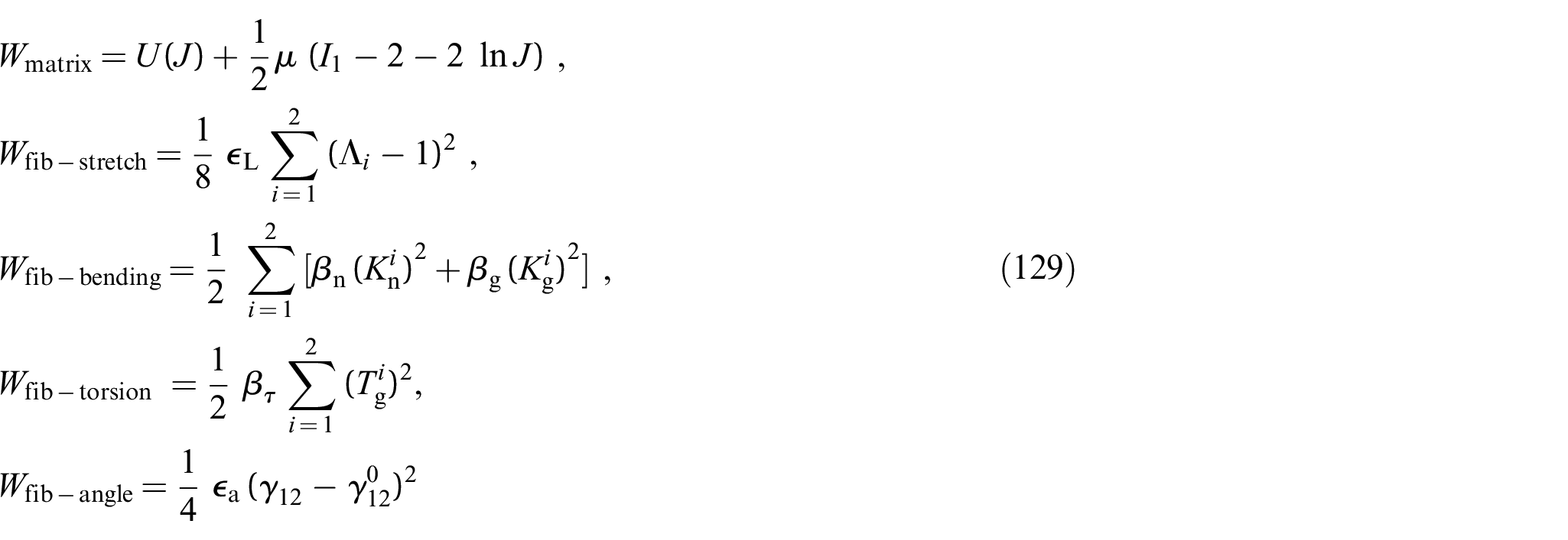
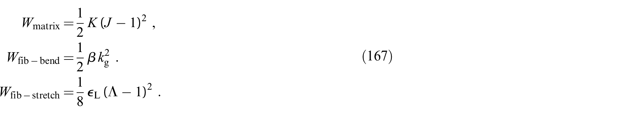
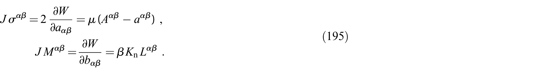
A simple generalized shell model for two-fiber-family fabrics that are initially curved and bonded to a matrix is given by

$$W=W_{\mathrm{matrix}}+W_{\mathrm{fib}-\mathrm{stretch}}+W_{\mathrm{fib}-\mathrm{bending}}+W_{\mathrm{fib}-\mathrm{torsion}}+W_{\mathrm{fib}-\mathrm{angle}},$$

(128)

where

$$\begin{array}{c}{W}_{\mathrm{matrix}}=U(J)+\frac{1}{2}\mu (I_1-2-2\ln J),\hfill \\ W_{\mathrm{fib}-\mathrm{stretch}}=\frac{1}{8}{ϵ}_{\mathrm{L}}\sum _{i=1}^2({\mathrm{\Lambda }}_i-1{)}^2,\hfill \\ W_{\mathrm{fib}-\mathrm{bending}}=\frac{1}{2}\sum _{i=1}^2[{\beta }_{\mathrm{n}}{(K_{\mathrm{n}}^i)}^2+{\beta }_{\mathrm{g}}{(K_{\mathrm{g}}^i)}^2],\hfill \\ W_{\mathrm{fib}-\mathrm{torsion}}=\frac{1}{2}{\beta }_{\tau }\sum _{i=1}^2(T_{\mathrm{g}}^i{)}^2,\hfill \\ W_{\mathrm{fib}-\mathrm{angle}}=\frac{1}{4}{ϵ}_{\mathrm{a}}({\gamma }_{12}-{\gamma }_{12}^0{)}^2\hfill \end{array}$$

(129)

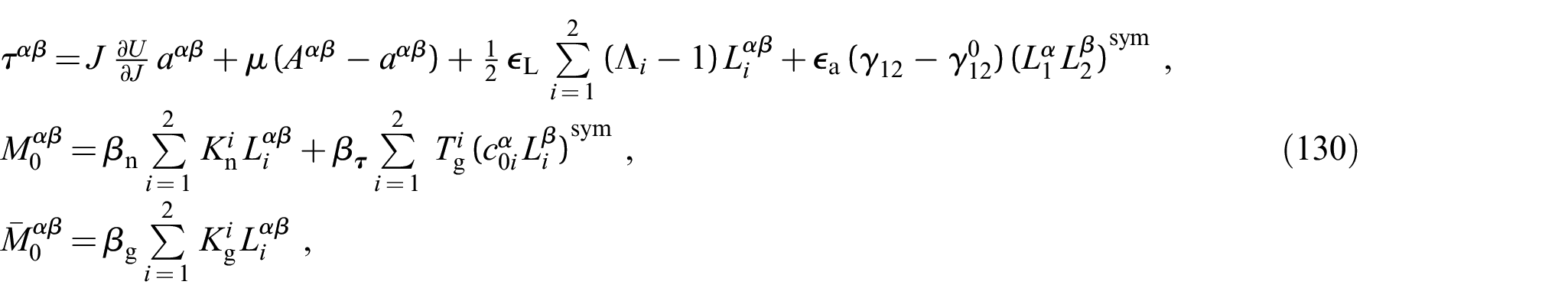
are the strain energies for matrix deformation, fiber stretching, out-of-plane and in-plane fiber bending, fiber torsion, and the linkage between the two fiber families, respectively. $U(J)$ is the surface dilatation energy. In the above expression, $\sqrt{\mathrm{\Lambda }}$ , $T_{\mathrm{g}}$ , $K_{\mathrm{n}}$ , $K_{\mathrm{g}}$ , and ${\gamma }_{12}$ denote the fiber stretch, the norminal change in geodesic fiber torsion, normal fiber curvature and geodesic fiber curvature, and the relative angle between fiber families, respectively (see Tables 1 and 2). Symbols $\mu$ , ${ϵ}_{•}$ , and ${\beta }_{•}$ are material parameters. ${ϵ}_{\mathrm{L}}$ can be taken as zero during fiber compression ( ${\mathrm{\Lambda }}_i<1$ ) to mimic buckling phenomenologically.

From equations (116) and (129), we then find the effective stress and moment components for the director gradient-based formulation (section 4.2) (see Appendix 2 and Sauer and Duong [10] for the required derivatives of kinematical quantities) as

$$\begin{array}{c}{\tau }^{\alpha \beta }=J\frac{\partial U}{\partial J}{a}^{\alpha \beta }+\mu (A^{\alpha \beta }-a^{\alpha \beta })+\frac{1}{2}{ϵ}_{\mathrm{L}}\sum _{i=1}^2({\mathrm{\Lambda }}_i-1)L_i^{\alpha \beta }+{ϵ}_{\mathrm{a}}({\gamma }_{12}-{\gamma }_{12}^0){(L_1^{\alpha }{L}_2^{\beta })}^{\mathrm{sym}},\hfill \\ \multicolumn{1}{c}{M_0^{\alpha \beta }={\beta }_{\mathrm{n}}\sum _{i=1}^2{K}_{\mathrm{n}}^i{L}_i^{\alpha \beta }+{\beta }_{\mathit{\tau }}\sum _{i=1}^2{T}_{\mathrm{g}}^i{(c_{0i}^{\alpha }{L}_i^{\beta })}^{\mathrm{sym}},}\\ \multicolumn{1}{c}{{\overline{M}}_0^{\alpha \beta }={\beta }_{\mathrm{g}}\sum _{i=1}^2{K}_{\mathrm{g}}^i{L}_i^{\alpha \beta },}\end{array}$$

(130)

where $({•}^{\alpha \beta }{)}^{\mathrm{sym}}=(\frac{1}{2})({•}^{\alpha \beta }+{•}^{\beta \alpha })$ denotes symmetrization.

5.2. Fiber inextensibility constraints

For most textile materials, the deformation is usually characterized by very high tensile stiffness in fiber direction and low in-plane shear and bending stiffness. In this case, one may model the very high tensile stiffness along the fiber direction $i$ by the inextensibility constraint

$$\begin{array}{c}{g}_i:={\mathrm{\Lambda }}_i-1=0,{\mathrm{\Lambda }}_i>1,\hfill \end{array}$$

(131)

where ${\mathrm{\Lambda }}_i$ is defined in Table 2. This constraint then replaces the $W_{\mathrm{fib}-\mathrm{stretch}}$ term in equation (128). To enforce this constraint, we can employ the Lagrange multiplier method in the strain energy function

$$\begin{array}{c}\hat{W}:=W+\sum _{i=1}^{n_{\mathrm{f}}}{q}_i{g}_i,\hfill \end{array}$$

(132)

where $q_i$ ( $i=1,...,n_{\mathrm{f}}$ ) denote the corresponding Lagrange multipliers. The stress components in this case become

$${\tau }^{\alpha \beta }=2\frac{\partial \hat{W}}{\partial a_{\alpha \beta }}=2\frac{\partial W}{\partial a_{\alpha \beta }}+\sum _{i=1}^{n_{\mathrm{f}}}2q_i{L}_i^{\alpha \beta }.$$

(133)

This leads to the same stress and moment components as in equation (130.1) with the exception that ${ϵ}_{\mathrm{L}}({\mathrm{\Lambda }}_i-1)/2$ is now replaced by $2q_i$ .

6. Weak form

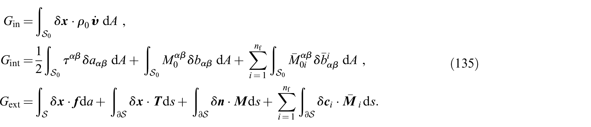
This section presents the weak form for the generalized Kirchhoff–Love shell. The weak form is obtained by the same steps as the mechanical power balance in section 3.5, simply by replacing velocity $\mathit{\upsilon }$ by variation $\delta x$ . This gives

$$\begin{array}{c}{G}_{\mathrm{in}}+G_{\mathrm{int}}-G_{\mathrm{ext}}=0\forall \delta \mathit{x}\in \mathcal{V},\hfill \end{array}$$

(134)

where according to equations (101), (102), (104), and (124)

$$\begin{array}{c}\multicolumn{1}{c}{G_{\mathrm{in}}={\int }_{{\mathcal{S}}_0}\delta \mathit{x}·{\rho }_0\stackrel{·}{\mathit{\upsilon }}\mathrm{d}A,}\\ \multicolumn{1}{c}{G_{\mathrm{int}}=\frac{1}{2}{\int }_{{\mathcal{S}}_0}{\tau }^{\alpha \beta }\delta a_{\alpha \beta }\mathrm{d}A+{\int }_{{\mathcal{S}}_0}{M}_0^{\alpha \beta }\delta b_{\alpha \beta }\mathrm{d}A+\sum _{i=1}^{n_{\mathrm{f}}}{\int }_{{\mathcal{S}}_0}{\overline{M}}_{0i}^{\alpha \beta }\delta {\overline{b}}_{\alpha \beta }^i\mathrm{d}A,}\\ \multicolumn{1}{c}{G_{\mathrm{ext}}={\int }_{\mathcal{S}}\delta \mathit{x}·\mathit{f}\mathrm{d}a+{\int }_{\partial \mathcal{S}}\delta \mathit{x}·\mathit{T}\mathrm{d}s+{\int }_{\partial \mathcal{S}}\delta \mathit{n}·\mathit{M}\mathrm{d}s+\sum _{i=1}^{n_{\mathrm{f}}}{\int }_{\partial \mathcal{S}}\delta {\mathit{c}}_i·{\overline{\mathit{M}}}_i\mathrm{d}s.}\end{array}$$

(135)

Using equation (127), $G_{\mathrm{int}}$ can also be expressed as the variation of potential (125) w.r.t. its arguments,

$$G_{\mathrm{int}}={\int }_{{\mathcal{S}}_0}\delta W\mathrm{d}A={\int }_{{\mathcal{S}}_0}\frac{\partial W}{\partial a_{\alpha \beta }}\delta a_{\alpha \beta }\mathrm{d}A+{\int }_{{\mathcal{S}}_0}\frac{\partial W}{\partial b_{\alpha \beta }}\delta b_{\alpha \beta }\mathrm{d}A+\sum _{i=1}^{n_{\mathrm{f}}}{\int }_{{\mathcal{S}}_0}\frac{\partial W}{\partial {\overline{b}}_{\alpha \beta }^i}\delta {\overline{b}}_{\alpha \beta }^i\mathrm{d}A.$$

(136)

For constrained materials, for example, equation (132), $G_{\mathrm{int}}$ becomes

$$G_{\mathrm{int}}={\int }_{{\mathcal{S}}_0}\delta \hat{W}\mathrm{d}A={\int }_{{\mathcal{S}}_0}(\frac{1}{2}{\tau }^{\alpha \beta }\delta a_{\alpha \beta }+M_0^{\alpha \beta }\delta b_{\alpha \beta }+\sum _{i=1}^{n_{\mathrm{f}}}{\overline{M}}_{0i}^{\alpha \beta }\delta {\overline{b}}_{\alpha \beta }^i)\mathrm{d}A+\sum _{i=1}^{n_{\mathrm{f}}}{\int }_{{\mathcal{S}}_0}\frac{\partial \hat{W}}{\partial q_i}\delta q_i\mathrm{d}A.$$

(137)

For the constitutive example in section 5, ${\tau }^{\alpha \beta }$ , $M_0^{\alpha \beta }$ and ${\overline{M}}_0^{\alpha \beta }$ are given by equations (133), (130.2), and (130.3), respectively, while $\partial \hat{W}/\partial q_i=g_i$ .

The linearization of weak form (134) and its discretization can be found in the work by Duong et al. [37].

7. Analytical solutions

This section illustrates the preceding theory by several analytical examples considering simple homogeneous deformation states. They are useful elementary test cases for the verification of computational formulations.

7.1. Geodesic curvature of a circle embedded in an expanding flat surface

The first example presents the computation of geodesic curvature ${\kappa }_{\mathrm{g}}$ from equations (51) and (52) and confirms that only equation (51) gives the correct value for initially curved fibers. This illustrates the limitation of existing second-gradient Kirchhoff–Love shell theory for cases where ${\stackrel{·}{\mathrm{\Gamma }}}_{\alpha \beta }^{\gamma }=0$ due to the choice of the surface parametrization.

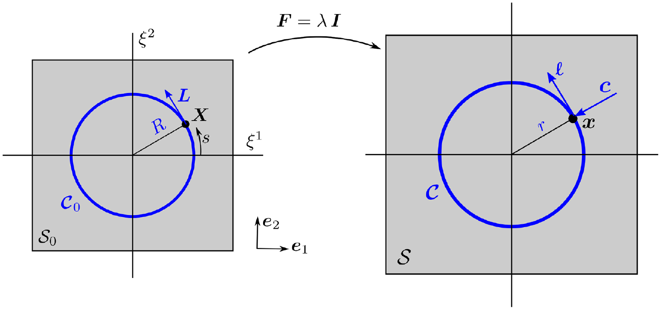
To this end, we consider a circular fiber ${\mathcal{C}}_0\in {\mathcal{S}}_0$ with initial radius $R$ expanding according to the deformation gradient $\mathit{F}=\lambda \mathit{I}$ to $\mathcal{C}\in \mathcal{S}$ with the current radius $r$ as shown in Figure 3. Therefore, the geodesic curvatures of ${\mathcal{C}}_0$ and $\mathcal{C}$ are expected to simply be ${\kappa }_{\mathrm{g}}^0=1/R$ and ${\kappa }_{\mathrm{g}}=1/r$ , respectively.

Figure 3.

Computation of geodesic curvature ${\kappa }_{\mathrm{g}}$ : A circular fiber $\mathcal{C}$ is embedded in the planar surface $\mathcal{S}$ that is expanded by the homogeneous deformation $\mathit{F}=\lambda \mathit{I}$ .

With respect to the convective coordinates $({\xi }^1=X$ , ${\xi }^2=Y)$ shown in Figure (3(left)), the position vector on any point of ${\mathcal{S}}_0$ and $\mathcal{S}$ can be represented by

$$\begin{array}{c}\mathit{X}={\mathit{X}}_{\mathrm{s}}({\xi }^1,{\xi }^2):={\xi }^1{\mathit{e}}_1+{\xi }^2{\mathit{e}}_2,\hfill \\ \multicolumn{1}{c}{\mathit{x}={\mathit{x}}_{\mathrm{s}}({\xi }^1,{\xi }^2):=\lambda {\xi }^1{\mathit{e}}_1+\lambda {\xi }^2{\mathit{e}}_2.}\end{array}$$

(138)

The surface tangent and normal vectors follow from equation (138) as

$$\begin{array}{c}{\mathit{A}}_1={\mathit{e}}_1,{\mathit{A}}_2={\mathit{e}}_2,\mathrm{and}\mathit{N}={\mathit{e}}_3,\hfill \\ \multicolumn{1}{c}{{\mathit{a}}_1=\lambda {\mathit{e}}_1,{\mathit{a}}_2=\lambda {\mathit{e}}_2,\mathrm{and}\mathit{n}={\mathit{e}}_3,}\end{array}$$

(139)

so that

$$\begin{array}{c}{\mathit{A}}^1={\mathit{e}}_1,{\mathit{A}}^2={\mathit{e}}_2,\hfill \\ \multicolumn{1}{c}{{\mathit{a}}^1=\frac{1}{\lambda }{\mathit{e}}_1,{\mathit{a}}^2=\frac{1}{\lambda }{\mathit{e}}_2.}\end{array}$$

(140)

The surface deformation gradient then reads

$$\mathit{F}={\mathit{a}}_{\alpha }\otimes {\mathit{A}}^{\alpha }=\lambda ({\mathit{e}}_1\otimes {\mathit{e}}_1+{\mathit{e}}_2\otimes {\mathit{e}}_2),$$

(141)

and the surface Christoffel symbols take the form

$${\overline{\mathrm{\Gamma }}}_{\alpha \beta }^{\gamma }:={\mathit{A}}_{\alpha ,\beta }·{\mathit{A}}^{\gamma }=0,{\mathrm{\Gamma }}_{\alpha \beta }^{\gamma }:={\mathit{a}}_{\alpha ,\beta }·{\mathit{a}}^{\gamma }=0.$$

(142)

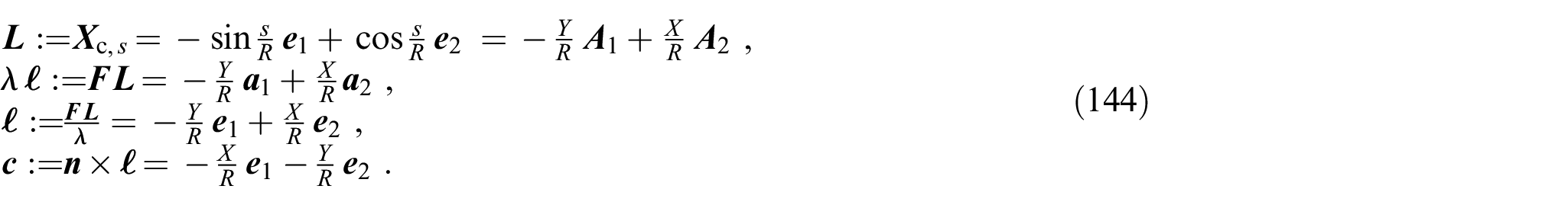
In the reference configuration, the fiber is parametrized by the arc-length coordinate $s$ as

$$\begin{array}{c}\mathit{X}={\mathit{X}}_{\mathrm{c}}(s):=R\cos \frac{s}{R}{\mathit{e}}_1+R\sin \frac{s}{R}{\mathit{e}}_2.\hfill \end{array}$$

(143)

From equations (143) and (141) follows

$$\begin{array}{c}\mathit{L}:={\mathit{X}}_{\mathrm{c},s}=-\sin \frac{s}{R}{\mathit{e}}_1+\cos \frac{s}{R}{\mathit{e}}_2=-\frac{Y}{R}{\mathit{A}}_1+\frac{X}{R}{\mathit{A}}_2,\hfill \\ \multicolumn{1}{c}{\lambda \mathit{\ell }:=\mathit{F}\mathit{L}=-\frac{Y}{R}{\mathit{a}}_1+\frac{X}{R}{\mathit{a}}_2,}\\ \multicolumn{1}{c}{\mathit{\ell }:=\frac{\mathit{F}\mathit{L}}{\lambda }=-\frac{Y}{R}{\mathit{e}}_1+\frac{X}{R}{\mathit{e}}_2,}\\ \multicolumn{1}{c}{\mathit{c}:=\mathit{n}\times \mathit{\ell }=-\frac{X}{R}{\mathit{e}}_1-\frac{Y}{R}{\mathit{e}}_2.}\end{array}$$

(144)

In this equation $({\xi }^1,{\xi }^2)=(X,Y)\in {\mathcal{C}}_0$ . Thus,

$$[{\hat{L}}_{,\beta }^{\alpha }]:=\frac{1}{\lambda }[L_{,\beta }^{\alpha }]=\frac{1}{\lambda R}\left[\begin{array}{cc}0\hfill & -1\hfill \\ \multicolumn{1}{c}{1}& 0\hfill \end{array}\right],$$

(145)

and

$$[{\ell }^{\alpha }]:=[\mathit{\ell }·{\mathit{a}}^{\alpha }]=\frac{1}{\lambda R}\left[\begin{array}{c}-Y\hfill \\ \multicolumn{1}{c}{X}\end{array}\right],[c_{\alpha }]:=[\mathit{c}·{\mathit{a}}_{\alpha }]=-\frac{\lambda }{R}\left[\begin{array}{c}X\hfill \\ \multicolumn{1}{c}{Y}\end{array}\right].$$

(146)

Inserting these expressions into equation (51), and using the identity $X^2+Y^2=R^2$ gives the geodesic curvature

$${\kappa }_{\mathrm{g}}^{\mathrm{\Gamma }}=0,{\kappa }_{\mathrm{g}}^{\mathrm{L}}=\frac{1}{\lambda R}=\frac{1}{r},{\kappa }_{\mathrm{g}}={\kappa }_{\mathrm{g}}^{\mathrm{\Gamma }}+{\kappa }_{\mathrm{g}}^{\mathrm{L}}=\frac{1}{r}.$$

(147)

For ${\mathcal{C}}_0$ , setting $\lambda =1$ directly yields ${\kappa }_{\mathrm{g}}^0=1/R$ .

In contrast, equation (52) obviously fails to reproduce the correct geodesic curvatures since the Christoffel symbols are zero everywhere solely due to the choice of the surface parametrization. Furthermore, since ${\stackrel{·}{\mathrm{\Gamma }}}_{\alpha \beta }^{\gamma }=0$ , the in-plane bending term of the internal power is ill-defined in second-gradient theory (equation (123)), whereas we get a well-defined power from equation (51) with equations (103), (107), and (113). It correctly captures the change in geodesic curvature.

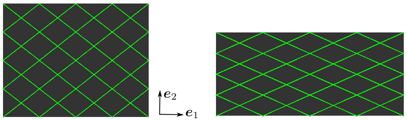
7.2. Biaxial stretching of a sheet containing diagonal fibers

The second example presents an analytical solution for homogeneous biaxial stretching of a rectangular sheet from dimension $L\times H$ to $\ell \times h$ , such that $\ell ={\lambda }_{\ell }L$ and $h={\lambda }_{h}H$ . The sheet contains a matrix material and two fiber families distributed diagonally as shown in Figure 4. The strain energy function in this example is taken from equation (129) as

$$W=\frac{\mu }{2}(I_1-2-\ln J)+\frac{1}{8}{ϵ}_{\mathrm{L}}\sum _{i=1}^2({\mathrm{\Lambda }}_i-1{)}^2+\frac{1}{4}{ϵ}_{\mathrm{a}}({\gamma }_{12}-{\gamma }_{12}^0{)}^2.$$

(148)

Figure 4.

Biaxial stretching of a rectangular sheet from dimension $L\times H$ (left) to $\ell \times h$ (right).

Therefore, the stress components follow as

$${\tau }^{\alpha \beta }=\mu (A^{\alpha \beta }-a^{\alpha \beta })+\sum _{i=1}^2{\tau }_i{L}_i^{\alpha \beta }+{ϵ}_{\mathrm{a}}({\gamma }_{12}-{\gamma }_{12}^0)(L_1^{\alpha }{L}_2^{\beta }{)}^{\mathrm{sym}},$$

(149)

where ${\tau }_i:=\frac{1}{2}{ϵ}_{\mathrm{L}}({\mathrm{\Lambda }}_i-1)$ denotes the nominal fiber tension. The parameterization can be chosen such that the surface tangent vectors are ${\mathit{A}}_1=L{\mathit{e}}_1$ , ${\mathit{A}}_2=H{\mathit{e}}_2$ , ${\mathit{a}}_1=\ell {\mathit{e}}_1$ , and ${\mathit{a}}_2=h{\mathit{e}}_2$ , where $e_{\alpha }$ are the basis vectors shown in Figure 4. The fiber directions are ${\mathit{L}}_1=(L{\mathit{e}}_1+H{\mathit{e}}_2)/D$ , ${\mathit{L}}_2=(L{\mathit{e}}_1-H{\mathit{e}}_2)/D$ , where $D^2:=L^2+H^2$ . We thus find

$$\begin{array}{c}[A^{\alpha \beta }]=\left[\begin{array}{cc}1/L^2\hfill & 0\hfill \\ \multicolumn{1}{c}{0}& 1/H^2\hfill \end{array}\right],[a^{\alpha \beta }]=\left[\begin{array}{cc}1/{\ell }^2\hfill & 0\hfill \\ \multicolumn{1}{c}{0}& 1/h^2\hfill \end{array}\right],[L_1^{\alpha \beta }]=\frac{1}{D^2}\left[\begin{array}{cc}1\hfill & 1\hfill \\ \multicolumn{1}{c}{1}& 1\hfill \end{array}\right],\hfill \\ [L_2^{\alpha \beta }]=\frac{1}{D^2}\left[\begin{array}{cc}1\hfill & -1\hfill \\ \multicolumn{1}{c}{-1}& 1\hfill \end{array}\right],\mathrm{and}[L_1^{\alpha }{L}_2^{\beta }{]}^{\mathrm{sym}}=\frac{1}{D^2}\left[\begin{array}{cc}1\hfill & 0\hfill \\ \multicolumn{1}{c}{0}& -1\hfill \end{array}\right].\hfill \end{array}$$

(150)

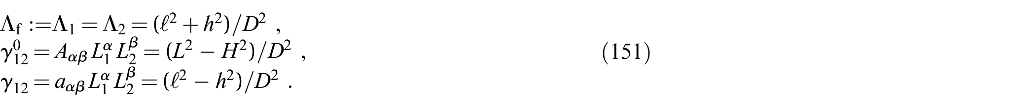
Furthermore, we find the fiber stretch and angles

$$\begin{array}{c}{\mathrm{\Lambda }}_{\mathrm{f}}:={\mathrm{\Lambda }}_1={\mathrm{\Lambda }}_2=({\ell }^2+h^2)/D^2,\hfill \\ \multicolumn{1}{c}{{\gamma }_{12}^0=A_{\alpha \beta }{L}_1^{\alpha }{L}_2^{\beta }=(L^2-H^2)/D^2,}\\ \multicolumn{1}{c}{{\gamma }_{12}=a_{\alpha \beta }{L}_1^{\alpha }{L}_2^{\beta }=({\ell }^2-h^2)/D^2.}\end{array}$$

(151)

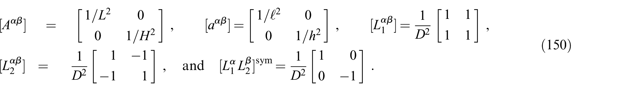
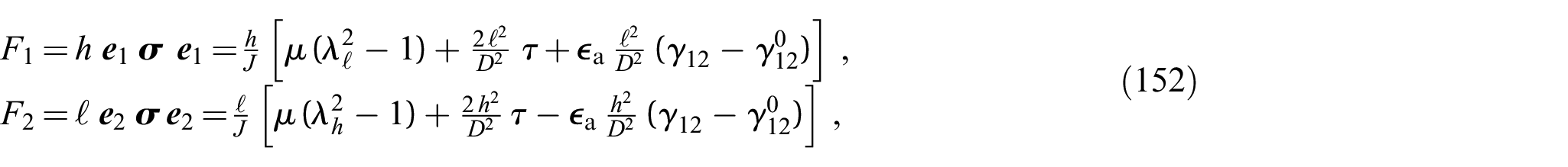
Inserting equation (151) into equation (149) gives the stress tensor $\mathbf{\sigma }=J^{-1}{\tau }^{\alpha \beta }{\mathit{a}}_{\alpha }\otimes {\mathit{a}}_{\beta }$ , where $J:={\lambda }_{\ell }{\lambda }_h$ The resultant reaction forces at the boundaries then follow as

$$\begin{array}{c}{F}_1=h{\mathit{e}}_1\mathbf{\sigma }{\mathit{e}}_1=\frac{h}{J}[\mu ({\lambda }_{\ell }^2-1)+\frac{2{\ell }^2}{D^2}\tau +{ϵ}_{\mathrm{a}}\frac{{\ell }^2}{D^2}({\gamma }_{12}-{\gamma }_{12}^0)],\hfill \\ \multicolumn{1}{c}{F_2=\ell {\mathit{e}}_2\mathbf{\sigma }{\mathit{e}}_2=\frac{\ell }{J}[\mu ({\lambda }_h^2-1)+\frac{2h^2}{D^2}\tau -{ϵ}_{\mathrm{a}}\frac{h^2}{D^2}({\gamma }_{12}-{\gamma }_{12}^0)],}\end{array}$$

(152)

where $\tau :={\tau }_1={\tau }_2=\frac{1}{2}{ϵ}_{\mathrm{L}}({\mathrm{\Lambda }}_{\mathrm{f}}-1)$ .

Remark 7.1. The presented solution (152) includes pure shear by simply setting ${\lambda }_h=1/{\lambda }_{\ell }$ .

Remark 7.2. For uniaxial tension, for example, in the ${\mathit{e}}_1$ direction and with free horizontal boundaries, condition $F_2=0$ in equation (152.2) gives the solution of ${\lambda }_h$ , which in turn can be inserted to equation (152.1) for the resultant reaction force $F_1({\lambda }_{\ell })$ as

$$F_1=\frac{H}{{\lambda }_{\ell }{D}^4}[D^4\mu ({\lambda }_{\ell }^2-1)+({ϵ}_{\mathrm{L}}+{ϵ}_{\mathrm{a}}){\lambda }_{\ell }^4{L}^4+({ϵ}_{\mathrm{L}}-{ϵ}_{\mathrm{a}}){\lambda }_{\ell }^2{\lambda }_h^2{H}^2{L}^2+({ϵ}_{\mathrm{L}}-{\gamma }_{12}^0{ϵ}_{\mathrm{a}}){\lambda }_{\ell }^2{L}^2{D}^2],$$

(153)

where

$${\lambda }_h^2=\frac{1}{2a}(-b+\sqrt{b^2+4a\mu }),$$

(154)

while $a:=\frac{H^2}{D^4}({ϵ}_{\mathrm{L}}+{ϵ}_{\mathrm{a}})$ , and $b:=\mu +({ϵ}_{\mathrm{L}}-{ϵ}_{\mathrm{a}})\frac{{\lambda }_{\ell }^2{L}^2{H}^2}{D^4}-{ϵ}_{\mathrm{L}}\frac{H^2}{D^2}+{\gamma }_{12}^0{ϵ}_{\mathrm{a}}\frac{H^2}{D^2}$ .

Remark 7.3. Solution (152) also captures the inextensibility of fibers. In this case, either the vertical or the horizontal boundaries have to be stress free. In the latter case, $F_2=0$ and

$${\lambda }_h=\sqrt{\frac{D^2}{H^2}-{\lambda }_{\ell }^2\frac{L^2}{H^2}},$$

(155)

due to $D^2={\ell }^2+h^2$ . In this case, the deformation is limited by ${\lambda }_{\ell }^{\max }=D/L$ . From $F_2=0$ , the nominal fiber tension now follows as

$$\tau =\frac{1}{2}{ϵ}_{\mathrm{a}}({\gamma }_{12}-{\gamma }_{12}^0)-\frac{1}{2}\frac{D^2}{h^2}\mu ({\lambda }_h^2-1).$$

(156)

Inserting equation (156) into equation (152.1) then gives

$$F_1=\frac{h}{J}[\mu ({\lambda }_{\ell }^2-1)-\frac{{\ell }^2}{h^2}\mu ({\lambda }_h^2-1)+2{ϵ}_{\mathrm{a}}\frac{{\ell }^2}{D^2}({\gamma }_{12}-{\gamma }_{12}^0)].$$

(157)

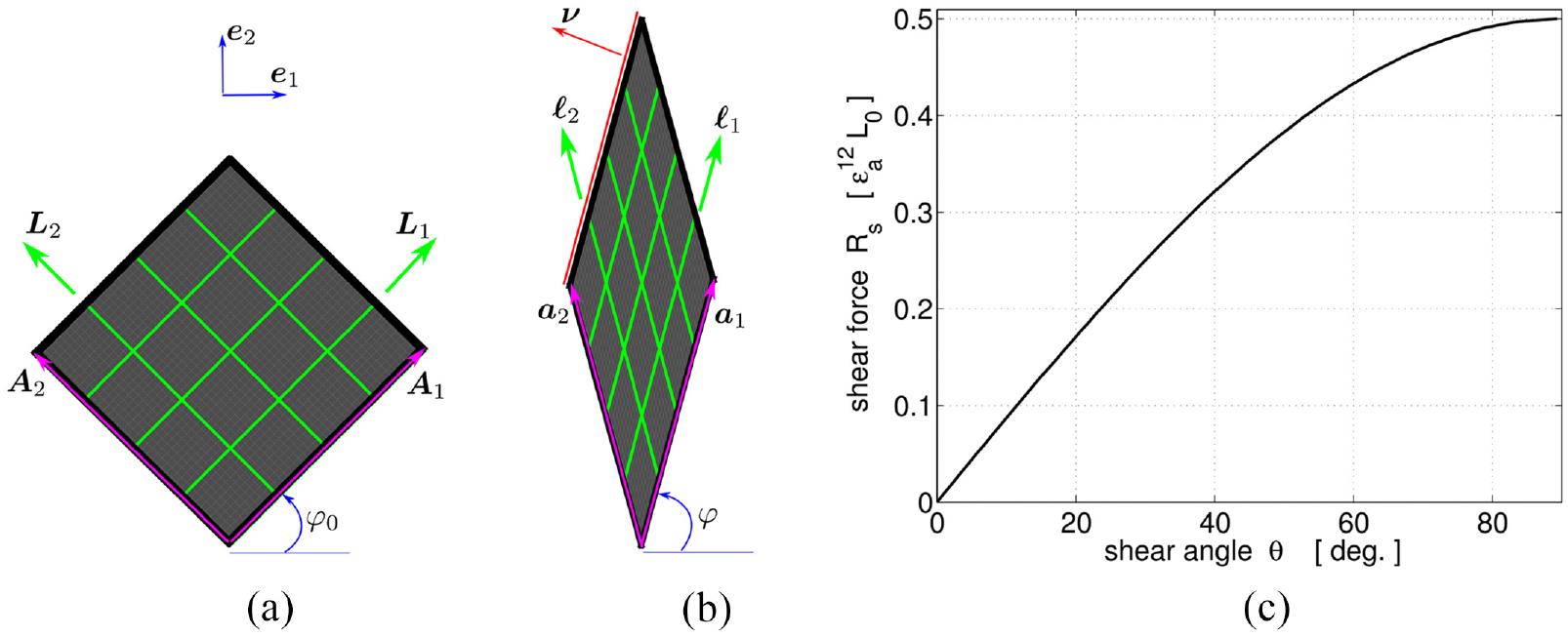
7.3. Picture frame test

The third example derives an analytical solution for the shear force in the picture frame test of an $L_0\times L_0$ square sheet with two fiber families as shown in Figure 5(a) and (b). From the figure, we find the surface tangent vectors

$$\begin{array}{c}{\mathit{A}}_1=L_0\cos {\phi }_0{\mathit{e}}_1+L_0\sin {\phi }_0{\mathit{e}}_2,{\mathit{a}}_1=L_0\cos \phi {\mathit{e}}_1+L_0\sin \phi {\mathit{e}}_2,\hfill \\ {\mathit{A}}_2=-L_0\cos {\phi }_0{\mathit{e}}_1+L_0\sin {\phi }_0{\mathit{e}}_2,{\mathit{a}}_2=-L_0\cos \phi {\mathit{e}}_1+L_0\sin \phi {\mathit{e}}_2,\hfill \end{array}$$

(158)

and the fiber directions

$$\begin{array}{c}{\mathit{L}}_1=\cos {\phi }_0{\mathit{e}}_1+\sin {\phi }_0{\mathit{e}}_2,{\mathit{\ell }}_1=\cos \phi {\mathit{e}}_1+\sin \phi {\mathit{e}}_2,\hfill \\ {\mathit{L}}_2=-\cos {\phi }_0{\mathit{e}}_1+\sin {\phi }_0{\mathit{e}}_2,{\mathit{\ell }}_2=-\cos \phi {\mathit{e}}_1+\sin \phi {\mathit{e}}_2,\hfill \end{array}$$

(159)

where ${\phi }_0=\pi /4$ . Accordingly, the components of tensors $\mathit{C}$ and $({\mathit{L}}_1\otimes {\mathit{L}}_2{)}^{\mathrm{sym}}$ read

$$\begin{array}{c}[C_{\alpha }^{\beta }]=a_{\alpha \gamma }{A}^{\gamma \beta }=\left[\begin{array}{cc}1\hfill & -\cos (2\phi )\hfill \\ \multicolumn{1}{c}{-\cos (2\phi )}& 1\hfill \end{array}\right],\mathrm{and}{[L_1^{\alpha }{L}_2^{\beta }]}^{\mathrm{sym}}=\frac{1}{2L_0^2}\left[\begin{array}{cc}0\hfill & 1\hfill \\ \multicolumn{1}{c}{1}& 0\hfill \end{array}\right],\hfill \end{array}$$

(160)

respectively. From equation (160.1), the surface stretch is found as

$$J=\sqrt{det[C_{\alpha }^{\beta }]}=\sin (2\phi ).$$

(161)

Figure 5.

Picture frame test: (a) initial and (b) deformed configurations containing two fiber families. (c) Exact solution of the shear force versus shear angle $\theta :=2\phi -{90}^{°}$ .

Furthermore, the strain energy function in this example is taken from equation (129) as $W=\frac{1}{4}{ϵ}_{\mathrm{a}}({\gamma }_{12}-{\gamma }_{12}^0{)}^2$ , so that the Cauchy stress components are

$$[{\sigma }^{\alpha \beta }]=\frac{1}{J}{ϵ}_{\mathrm{a}}({\gamma }_{12}-{\gamma }_{12}^0)[L_1^{\alpha }{L}_2^{\beta }{]}^{\mathrm{sym}}=-\frac{1}{2L_0^2}{ϵ}_{\mathrm{a}}\cot (2\phi )\left[\begin{array}{cc}0\hfill & 1\hfill \\ \multicolumn{1}{c}{1}& 0\hfill \end{array}\right].$$

(162)

Here, we have used equations (160.2) and (161), ${\gamma }_{12}^0={\mathit{L}}_1·{\mathit{L}}_2=0$ , and ${\gamma }_{12}={\mathit{\ell }}_1·{\mathit{\ell }}_2=-\cos (2\phi )$ .

Consider the upper left edge with normal vector $\mathit{\nu }=-\sin \phi {\mathit{e}}_1+\cos \phi {\mathit{e}}_2={\nu }_{\alpha }{\mathit{a}}^{\alpha }$ , where ${\nu }_1=\mathit{\nu }·{\mathit{a}}_1=0$ , and ${\nu }_2=\mathit{\nu }·{\mathit{a}}_2=L_0\sin (2\phi )$ . The traction components on this edge can be computed from

$$[t^{\alpha }]=[{\sigma }^{\alpha \beta }{\nu }_{\beta }]=-\frac{1}{2L_0}{ϵ}_{\mathrm{a}}^{12}\cos (2\phi )\left[\begin{array}{c}1\hfill \\ \multicolumn{1}{c}{0}\end{array}\right].$$

(163)

Therefore, the traction vector solely contains the shear contribution

$$\mathit{t}=t^{\alpha }{\mathit{a}}_{\alpha }=t^1{\mathit{a}}_1=-\frac{1}{2}{ϵ}_{\mathrm{a}}^{12}\cos (2\phi )(\cos \phi {\mathit{e}}_1+\sin \phi {\mathit{e}}_2),$$

(164)

so that the shear force (i.e. the tangential reaction) at the edge of the sheet is

$$R_{\mathrm{s}}=\mathit{t}·\frac{{\mathit{a}}_1}{\parallel {\mathit{a}}_1\parallel }{L}_0=-\frac{1}{2}{ϵ}_{\mathrm{a}}^{12}\cos (2\phi )L_0=\frac{1}{2}{ϵ}_{\mathrm{a}}^{12}\sin (\theta )L_0,$$

(165)

where $\theta :=2\phi -{90}^{°}$ denotes the shear angle. This solution is plotted in Figure 5(c).

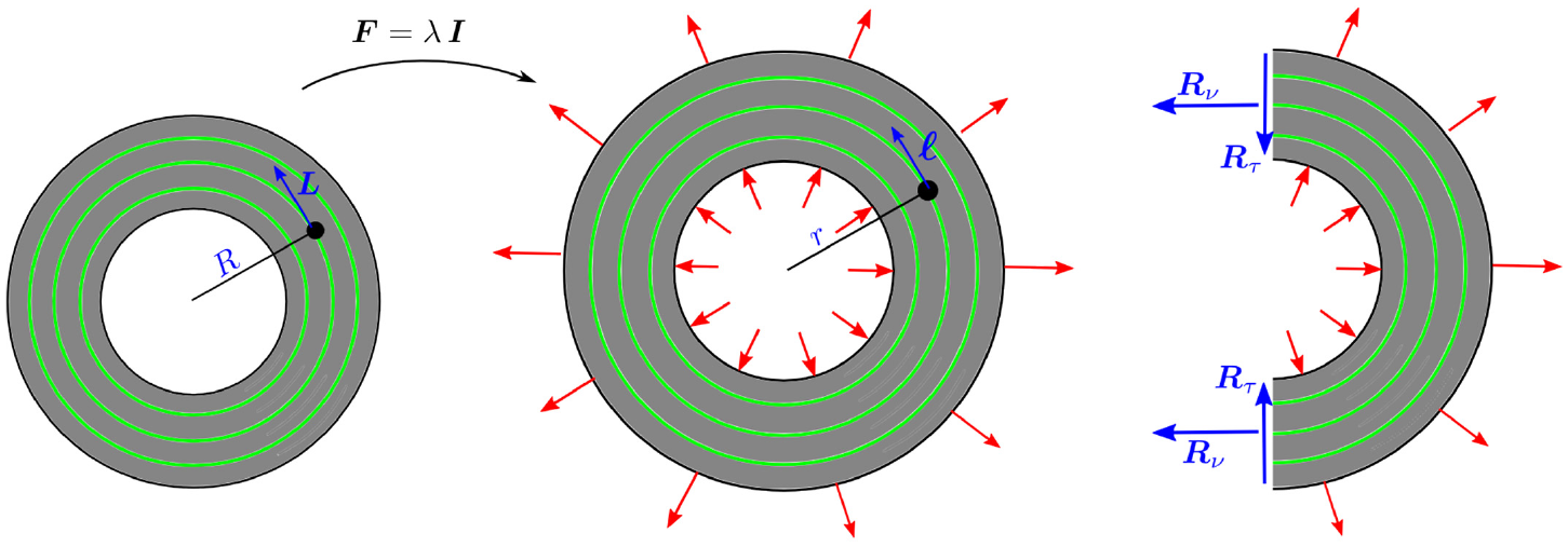
7.4. Annulus expansion

The fourth example presents an analytical solution for the expansion of an annulus containing distributed circular fibers and matrix material as depicted in Figure 6.

Figure 6.

Annulus expansion: An annulus containing matrix (gray color) and distributed circular fibers (green color) is expanded homogeneously from its initial configuration (left) by applying Dirichlet boundary condition on both inner and outer surfaces (middle). The expansion causes the resultant interface forces ${\mathit{R}}_{\nu }$ and ${\mathit{R}}_{\tau }$ on the cut through a symmetry plane (right).

The inner and the outer rings with radius $R_{\mathrm{i}}$ and $R_{\mathrm{o}}$ , respectively, are expanded to $r_{\mathrm{i}}$ and $r_{\mathrm{o}}$ by the constant stretch $\overline{\lambda }=r_{\mathrm{i}}/R_{\mathrm{i}}=r_{\mathrm{o}}/R_{\mathrm{o}}$ . The strain energy density (per reference area) is taken as

$$W=W_{\mathrm{matrix}}+W_{\mathrm{fib}-\mathrm{bend}}+W_{\mathrm{fib}-\mathrm{stretch}},$$

(166)

where

$$\begin{array}{c}\multicolumn{1}{c}{W_{\mathrm{matrix}}=\frac{1}{2}K{(J-1)}^2,}\\ \multicolumn{1}{c}{W_{\mathrm{fib}-\mathrm{bend}}=\frac{1}{2}\beta k_{\mathrm{g}}^2.}\\ \multicolumn{1}{c}{W_{\mathrm{fib}-\mathrm{stretch}}=\frac{1}{8}{ϵ}_{\mathrm{L}}{(\mathrm{\Lambda }-1)}^2.}\end{array}$$

(167)

Here, $K(R)$ , $\beta$ , and ${ϵ}_{\mathrm{L}}$ are material parameters for matrix dilatation, fiber bending, and fiber stretching, respectively, and $J$ , $\mathrm{\Lambda }$ , and $k_{\mathrm{g}}$ are invariants induced by tensors $\mathit{C}$ and $\overline{\mathit{K}}$ as listed in Tables 1 and 2.

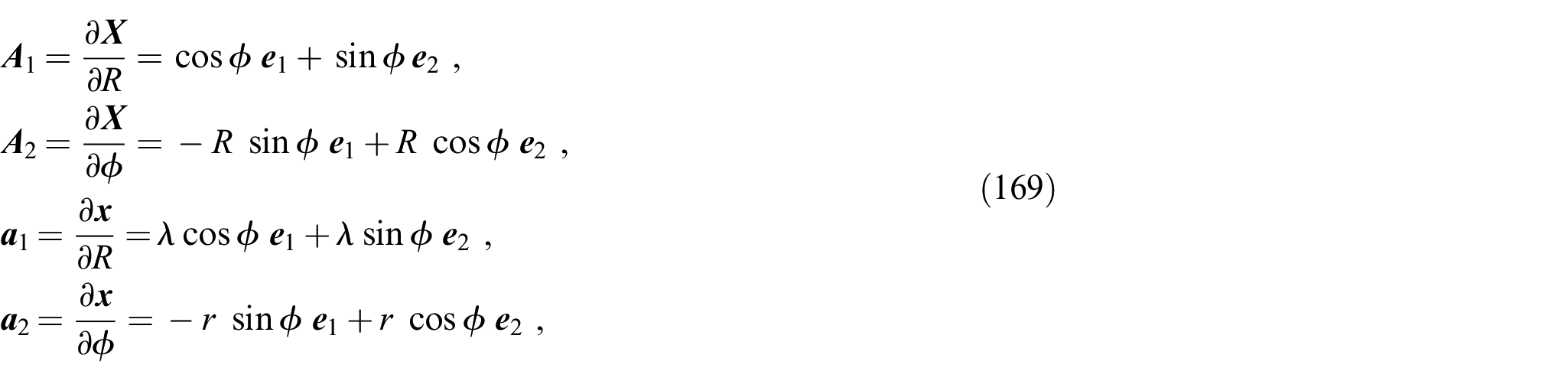
7.4.1. Kinematical quantities

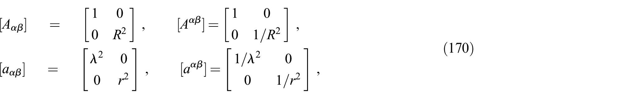
According to Figure 6, the initial and current configurations as well as the initial fiber direction can be described by

$$\begin{array}{c}\mathit{X}=\mathit{X}(R,\varphi ):=R\cos \varphi {\mathit{e}}_1+R\sin \varphi {\mathit{e}}_2,\hfill \\ \multicolumn{1}{c}{\mathit{x}=\mathit{x}(R,\varphi ):=r\cos \varphi {\mathit{e}}_1+r\sin \varphi {\mathit{e}}_2,}\\ \multicolumn{1}{c}{\mathit{L}=\mathit{L}(\varphi ):=-\sin \varphi {\mathit{e}}_1+\cos \varphi {\mathit{e}}_2.}\end{array}$$

(168)

Here $r=\lambda R$ , due to the homogeneous deformation, with $\lambda$ being the fiber stretch. From this, we find the covariant tangent vectors

$$\begin{array}{c}{\mathit{A}}_1=\frac{\partial \mathit{X}}{\partial R}=\cos \varphi {\mathit{e}}_1+\sin \varphi {\mathit{e}}_2,\hfill \\ {\mathit{A}}_2=\frac{\partial \mathit{X}}{\partial \varphi }=-R\sin \varphi {\mathit{e}}_1+R\cos \varphi {\mathit{e}}_2,\hfill \\ {\mathit{a}}_1=\frac{\partial \mathit{x}}{\partial R}=\lambda \cos \varphi {\mathit{e}}_1+\lambda \sin \varphi {\mathit{e}}_2,\hfill \\ {\mathit{a}}_2=\frac{\partial \mathit{x}}{\partial \varphi }=-r\sin \varphi {\mathit{e}}_1+r\cos \varphi {\mathit{e}}_2,\hfill \end{array}$$

(169)

and the constant surface normal $\mathit{n}=\mathit{N}={\mathit{e}}_3$ during deformation. From the tangent vectors, we get

$$\begin{array}{c}[A_{\alpha \beta }]=\left[\begin{array}{cc}1\hfill & 0\hfill \\ \multicolumn{1}{c}{0}& R^2\hfill \end{array}\right],[A^{\alpha \beta }]=\left[\begin{array}{cc}1\hfill & 0\hfill \\ \multicolumn{1}{c}{0}& 1/R^2\hfill \end{array}\right],\hfill \\ [a_{\alpha \beta }]=\left[\begin{array}{cc}{\lambda }^2\hfill & 0\hfill \\ \multicolumn{1}{c}{0}& r^2\hfill \end{array}\right],[a^{\alpha \beta }]=\left[\begin{array}{cc}1/{\lambda }^2\hfill & 0\hfill \\ \multicolumn{1}{c}{0}& 1/r^2\hfill \end{array}\right],\hfill \end{array}$$

(170)

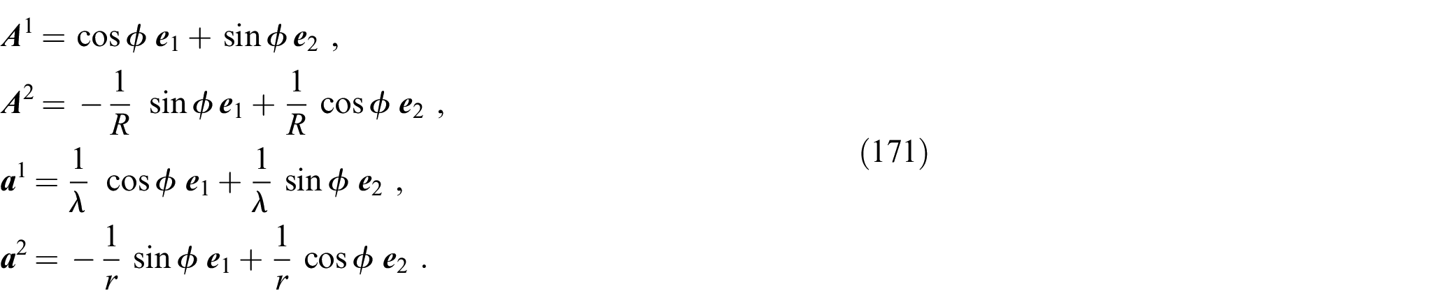
and thus the contravariant tangent vectors take the form

$$\begin{array}{c}{\mathit{A}}^1=\cos \varphi {\mathit{e}}_1+\sin \varphi {\mathit{e}}_2,\hfill \\ {\mathit{A}}^2=-\frac{1}{R}\sin \varphi {\mathit{e}}_1+\frac{1}{R}\cos \varphi {\mathit{e}}_2,\hfill \\ {\mathit{a}}^1=\frac{1}{\lambda }\cos \varphi {\mathit{e}}_1+\frac{1}{\lambda }\sin \varphi {\mathit{e}}_2,\hfill \\ {\mathit{a}}^2=-\frac{1}{r}\sin \varphi {\mathit{e}}_1+\frac{1}{r}\cos \varphi {\mathit{e}}_2.\hfill \end{array}$$

(171)

The initial and current fiber direction thus can be expressed as

$$\begin{array}{c}\mathit{L}=L^{\alpha }{\mathit{A}}_{\alpha },\hfill \\ \multicolumn{1}{c}{\mathit{\ell }=\frac{1}{\lambda }\mathit{F}\mathit{L}={\ell }^{\alpha }{\mathit{a}}_{\alpha },}\end{array}$$

(172)

with

$$[L^{\alpha }]:=[\mathit{L}·{\mathit{A}}^{\alpha }]=\left[\begin{array}{c}0\hfill \\ \multicolumn{1}{c}{1/R}\end{array}\right],\mathrm{and}[{\ell }^{\alpha }]:=[L^{\alpha }/\lambda ]=\left[\begin{array}{c}0\hfill \\ \multicolumn{1}{c}{1/r}\end{array}\right].$$

(173)

The components of the structural tensors $\mathit{L}\otimes \mathit{L}$ and $\mathit{\ell }\otimes \mathit{\ell }$ thus read

$$[L^{\alpha \beta }]=\left[\begin{array}{cc}0\hfill & 0\hfill \\ \multicolumn{1}{c}{0}& 1/R^2\hfill \end{array}\right],[{\ell }^{\alpha \beta }]=\left[\begin{array}{cc}0\hfill & 0\hfill \\ \multicolumn{1}{c}{0}& 1/r^2\hfill \end{array}\right],[{\ell }_{\beta }^{\alpha }]=\left[\begin{array}{cc}0\hfill & 0\hfill \\ \multicolumn{1}{c}{0}& 1\hfill \end{array}\right].$$

(174)

Furthermore, the fiber director is obtained as

$$\begin{array}{c}\mathit{c}=\mathit{n}\times \mathit{\ell }=-\cos \varphi {\mathit{e}}_1-\sin \varphi {\mathit{e}}_2=c_{\alpha }{\mathit{a}}^{\alpha },\hfill \end{array}$$

(175)

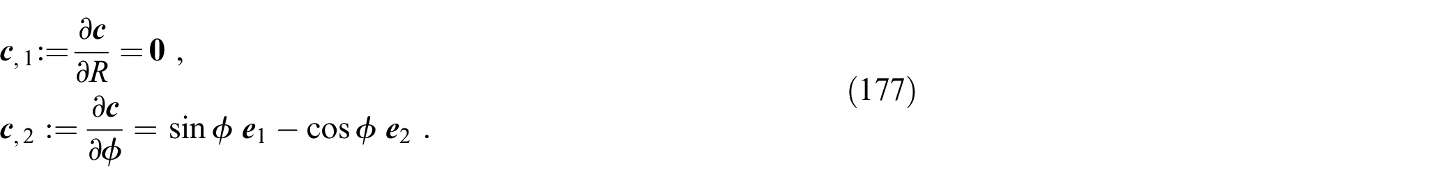
with

$$[c_{\alpha }]:=[\mathit{c}·{\mathit{a}}_{\alpha }]=\left[\begin{array}{c}-\lambda \hfill \\ \multicolumn{1}{c}{0}\end{array}\right].$$

(176)

Therefore, its derivatives read

$$\begin{array}{cc}\multicolumn{1}{c}{{\mathit{c}}_{,1}}& :=\frac{\partial \mathit{c}}{\partial R}=0,\hfill \\ \multicolumn{1}{c}{{\mathit{c}}_{,2}}& :=\frac{\partial \mathit{c}}{\partial \varphi }=\sin \varphi {\mathit{e}}_1-\cos \varphi {\mathit{e}}_2.\hfill \end{array}$$

(177)

From equation (35) then follow the components of the in-plane curvature tensor in the current configuration as

$$\begin{array}{c}[{\overline{b}}_{\alpha \beta }]=-\frac{1}{2}[{\mathit{c}}_{,\alpha }·{\mathit{a}}_{\beta }+{\mathit{c}}_{,\beta }·{\mathit{a}}_{\alpha }]=\left[\begin{array}{cc}0\hfill & 0\hfill \\ \multicolumn{1}{c}{0}& r\hfill \end{array}\right].\hfill \end{array}$$

(178)

Similarly, we find the in-plane curvature tensor in the initial configuration as

$$[{\overline{B}}_{\alpha \beta }]=\left[\begin{array}{cc}0\hfill & 0\hfill \\ \multicolumn{1}{c}{0}& R\hfill \end{array}\right].$$

(179)

Accordingly, the current geodesic curvature can be computed from equation (32) as

$${\kappa }_{\mathrm{g}}={\overline{b}}_{\alpha \beta }{\ell }^{\alpha \beta }=1/r.$$

(180)

Similarly, we can verify that the initial geodesic curvature satisfies ${\kappa }_{\mathrm{g}}^0=1/R$ . These results lead to $k_{\mathrm{g}}={\kappa }_{\mathrm{g}}\lambda -{\kappa }_{\mathrm{g}}^0=0$ , and thus $W_{\mathrm{fib}-\mathrm{bend}}=0$ due to the particular choice of strain energy (equation (167.2)). This means that the change in the geodesic curvature ${\kappa }_{\mathrm{g}}$ in this example is purely due to fiber stretching and not due to fiber bending.

7.4.2. Analytical expression for the reaction forces

From equation (166), we find the effective membrane stress

$$J{\sigma }^{\alpha \beta }=2\frac{\partial W}{\partial a_{\alpha \beta }}=K(J-1)J{a}^{\alpha \beta }+\frac{1}{2}{ϵ}_{\mathrm{L}}({\lambda }^2-1)L^{\alpha \beta }.$$

(181)

Here, the component of the Cauchy stress tensor is $N^{\alpha \beta }={\sigma }^{\alpha \beta }$ since $M^{\alpha \beta }={\overline{M}}^{\alpha \beta }=0$ (see equation (112) with equation (93)). Its mixed components thus read

$$[N_{\beta }^{\alpha }]=K(J-1)\left[\begin{array}{cc}1\hfill & 0\hfill \\ \multicolumn{1}{c}{0}& 1\hfill \end{array}\right]+\frac{{ϵ}_{\mathrm{L}}}{2J}({\lambda }^2-1)\left[\begin{array}{cc}0\hfill & 0\hfill \\ \multicolumn{1}{c}{0}& {\lambda }^2\hfill \end{array}\right],$$

(182)

where we have inserted $A^{\alpha \beta }$ and $L^{\alpha \beta }$ from equations (170) and (174), respectively. It can be verified that for a homogeneous deformation $J={\lambda }^2$ , the local equilibrium equation $\mathrm{di}{\mathrm{v}}_{\mathrm{s}}\mathbf{\sigma }=\mathrm{di}{\mathrm{v}}_{\mathrm{s}}(N^{\alpha \beta }{\mathit{a}}_{\alpha }\otimes {\mathit{a}}_{\beta })=0$ is satisfied for the functionally graded surface bulk modulus

$$K(R)=\frac{1}{2}{ϵ}_{\mathrm{L}}\ln R.$$

(183)

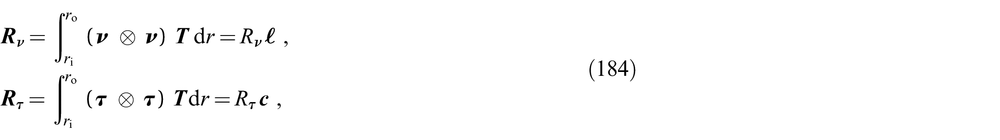
Furthermore, the resultant reaction force at the cut in Figure 6 (right) can be computed by

$$\begin{array}{c}{\mathit{R}}_{\nu }={\int }_{r_{\mathrm{i}}}^{r_{\mathrm{o}}}(\mathit{\nu }\otimes \mathit{\nu })\mathit{T}\mathrm{d}r=R_{\nu }\mathit{\ell },\hfill \\ {\mathit{R}}_{\mathit{\tau }}={\int }_{r_{\mathrm{i}}}^{r_{\mathrm{o}}}(\mathit{\tau }\otimes \mathit{\tau })\mathit{T}\mathrm{d}r=R_{\tau }\mathit{c},\hfill \end{array}$$

(184)

since $\mathit{\nu }=\mathit{\ell }$ and $\mathit{\tau }=\mathit{c}$ . Here, $\mathit{T}=N^{\alpha \beta }{\nu }_{\beta }{\mathit{a}}_{\alpha }$ denotes the traction acting on the cut. Therefore, we get

$$\begin{array}{c}\mathit{T}·\mathit{\ell }=N_{\beta }^{\alpha }{\mathit{\ell }}_{\alpha }^{\beta }=(\frac{1}{2}{ϵ}_{\mathrm{L}}+K)(J-1),\hfill \\ \mathit{T}·\mathit{c}=N_{\beta }^{\alpha }{c}_{\alpha }{\mathit{\ell }}^{\beta }=0.\hfill \end{array}$$

(185)

Inserting this into equation (184) and taking equation (183) into account finally results in

$$\begin{array}{c}{R}_{\nu }=\frac{1}{2}{ϵ}_{\mathrm{L}}(J-1)\overline{\lambda }(R_{\mathrm{o}}\ln R_{\mathrm{o}}-R_{\mathrm{i}}\ln R_{\mathrm{i}}),\hfill \\ R_{\tau }=0.\hfill \end{array}$$

(186)

7.5. Pure bending of a flat rectangular sheet

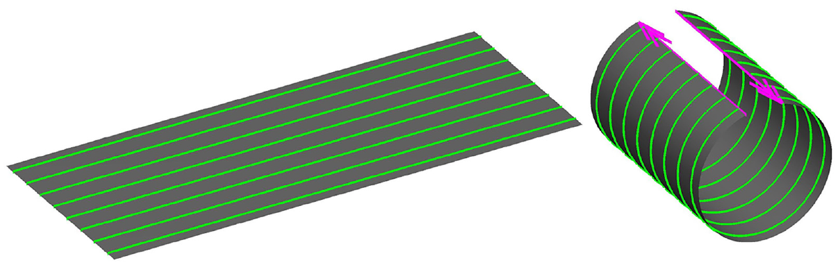
The last example presents the analytical solution for the pure bending of a flat rectangular sheet ${\mathcal{S}}_0$ with dimension $S\times L$ , subjected to an external bending moment $M_{\mathrm{ext}}$ along the two shorter edges, as shown in Figure 7. This problem was solved by Sauer and Duong [10] for an isotropic material, and here we additionally consider the influence of fiber bending. For simplicity the fibers are aligned along the bending direction. The strain energy function is taken from (129), which reduces to

$$W=\frac{\mu }{2}(I_1-2-\ln J)+\frac{\beta }{2}{K}_{\mathrm{n}}^2$$

(187)

in this example.

Figure 7.

Pure bending: Deformation of a rectangular sheet (left) into a circular arc (right).

7.5.1. Kinematical quantities

We extend the kinematical quantities derived in the work by Sauer and Duong [10] to account for embedded fibers. The sheet is parametrized by ${\xi }^1\in [0,S]$ and ${\xi }^2\in [0,L]$ . Bending induces (high-order) in-plane deformation, such that the current configuration $\mathcal{S}$ has dimension $s\times \ell$ . The stretches along the longer and shorter edges are ${\lambda }_{\ell }=\ell /L$ and ${\lambda }_s=s/S$ , respectively, and we have relations $\theta :={\kappa }_{\ell }{\lambda }_{\ell }\xi$ and $r:=1/{\kappa }_{\ell }$ , where ${\kappa }_{\ell }$ is the homogeneous curvature of the sheet.

With this, the sheet in the initial and current configurations, and the initial fiber direction can be described by

$$\begin{array}{c}\mathit{X}(\xi ,\eta )=\xi {\mathit{e}}_1+\eta {\mathit{e}}_2,\hfill \\ \multicolumn{1}{c}{\mathit{x}(\xi ,\eta )=r\sin \theta {\mathit{e}}_1+{\lambda }_s\eta {\mathit{e}}_2+r(1-\cos \theta ){\mathit{e}}_3,}\\ \multicolumn{1}{c}{\mathit{L}={\mathit{e}}_1.}\end{array}$$

(188)

Therefore, the initial and current tangent vectors, and current normal vector are

$$\begin{array}{c}{\mathit{A}}_1=\frac{\partial \mathit{X}}{\partial \xi }={\mathit{e}}_1,{\mathit{A}}_2=\frac{\partial \mathit{X}}{\partial \eta }={\mathit{e}}_2,\hfill \\ {\mathit{a}}_1=\frac{\partial \mathit{x}}{\partial \xi }={\lambda }_{\ell }(\cos \theta {\mathit{e}}_1+\sin \theta {\mathit{e}}_3),{\mathit{a}}_2=\frac{\partial x}{\partial \eta }={\lambda }_s{\mathit{e}}_2,\hfill \\ \mathit{n}=-\sin \theta {\mathit{e}}_1+\cos \theta {\mathit{e}}_3.\hfill \end{array}$$

(189)

From these, we find the components of the structural tensor

$$\begin{array}{c}[L^{\alpha \beta }]=[{\mathit{A}}^{\alpha }(\mathit{L}\otimes \mathit{L}){\mathit{A}}^{\beta }]=\left[\begin{array}{cc}1\hfill & 0\hfill \\ \multicolumn{1}{c}{0}& 0\hfill \end{array}\right],\hfill \end{array}$$

(190)

the surface metrics

$$\begin{array}{c}[A_{\alpha \beta }]=\left[\begin{array}{cc}1\hfill & 0\hfill \\ \multicolumn{1}{c}{0}& 1\hfill \end{array}\right],[A^{\alpha \beta }]=\left[\begin{array}{cc}1\hfill & 0\hfill \\ \multicolumn{1}{c}{0}& 1\hfill \end{array}\right],\hfill \end{array}$$

(191)

$$\begin{array}{c}[a_{\alpha \beta }]=\left[\begin{array}{cc}{\lambda }_{\ell }^2\hfill & 0\hfill \\ \multicolumn{1}{c}{0}& {\lambda }_s^2\hfill \end{array}\right],[a^{\alpha \beta }]=\left[\begin{array}{cc}{\lambda }_{\ell }^{-2}\hfill & 0\hfill \\ \multicolumn{1}{c}{0}& {\lambda }_s^{-2}\hfill \end{array}\right],\hfill \end{array}$$

(192)

the surface stretch $J={\lambda }_{\ell }{\lambda }_s,$ and the components of the curvature tensor

$$[b_{\alpha \beta }]=\left[\begin{array}{cc}{\kappa }_{\ell }{\lambda }_{\ell }^2\hfill & 0\hfill \\ \multicolumn{1}{c}{0}& 0\hfill \end{array}\right],[b_{\beta }^{\alpha }]=\left[\begin{array}{cc}{\kappa }_{\ell }\hfill & 0\hfill \\ \multicolumn{1}{c}{0}& 0\hfill \end{array}\right],[b^{\alpha \beta }]=\left[\begin{array}{cc}{\kappa }_{\ell }{\lambda }_{\ell }^{-2}\hfill & 0\hfill \\ \multicolumn{1}{c}{0}& 0\hfill \end{array}\right],H=\frac{{\kappa }_{\ell }}{2}.$$

(193)

Therefore, the nominal change in the normal curvature is

$$K_{\mathrm{n}}=b_{\alpha \beta }{L}^{\alpha \beta }={\kappa }_{\ell }{\lambda }_{\ell }^2$$

(194)

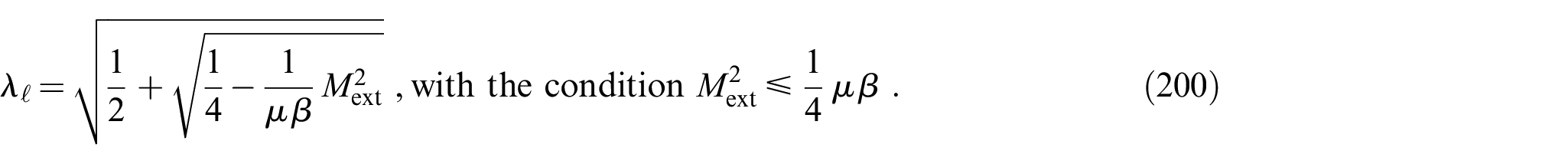
7.5.2. Analytical relation between external moment and mean curvature

From equation (187), we find

$$\begin{array}{c}\multicolumn{1}{c}{J{\sigma }^{\alpha \beta }=2\frac{\partial W}{\partial a_{\alpha \beta }}=\mu (A^{\alpha \beta }-a^{\alpha \beta }),}\\ \multicolumn{1}{c}{J{M}^{\alpha \beta }=\frac{\partial W}{\partial b_{\alpha \beta }}=\beta K_{\mathrm{n}}{L}^{\alpha \beta }.}\end{array}$$

(195)

According to equations (93) and (112) with ${\overline{M}}^{\alpha \beta }={\overline{m}}_{;\alpha }^{\alpha }=0$ , the components of the Cauchy stress tensors read

$$N_{\beta }^{\alpha }={\sigma }^{\alpha \gamma }{a}_{\gamma \beta }+M^{\alpha \gamma }{b}_{\gamma \beta }.$$

(196)

Inserting here $A^{\alpha \beta }$ , $a^{\alpha \beta }$ , and $L^{\alpha \beta }$ from equations (191), (192), and (190) gives

$$[N_{\beta }^{\alpha }]=\frac{\mu }{J}\left[\begin{array}{cc}{\lambda }_{\ell }^2-1\hfill & 0\hfill \\ \multicolumn{1}{c}{0}& {\lambda }_s^2-1\hfill \end{array}\right]+\frac{\beta }{J}{\kappa }_{\ell }^2{\lambda }_{\ell }^4\left[\begin{array}{cc}1\hfill & 0\hfill \\ \multicolumn{1}{c}{0}& 0\hfill \end{array}\right].$$

(197)

By assuming free edges, we have $N_1^1=N_2^2=0$ . That is

$$\begin{array}{c}{N}_1^1=\frac{\mu }{J}({\lambda }_{\ell }^2-1)+\frac{\beta }{J}{\kappa }_{\ell }^2{\lambda }_{\ell }^4=0,\hfill \\ \multicolumn{1}{c}{N_2^2=\frac{\mu }{J}({\lambda }_s^2-1)=0.}\end{array}$$

(198)

From the second equation follows ${\lambda }_s=1$ . The distributed external moment $M_{\mathrm{ext}}$ is in equilibrium to the distributed internal moment $m_{\tau }$ —see equation (79.2)—on any cut parallel to the shorter edge. We therefore have

$$M_{\mathrm{ext}}=-m_{\tau }=M^{\alpha \beta }{\nu }_{\alpha }{\nu }_{\beta }=\frac{\beta }{J}{\kappa }_{\ell }{\lambda }_{\ell }^4,$$

(199)

where $\mathit{\nu }={\mathit{a}}_1/{\lambda }_{\ell }$ , ${\nu }_1={\lambda }_{\ell }$ , and ${\nu }_2=0$ . By combining equations (199) and (198.1), we get an expression for ${\lambda }_{\ell }$ in terms of $M_{\mathrm{ext}}$

$${\lambda }_{\ell }=\sqrt{\frac{1}{2}+\sqrt{\frac{1}{4}-\frac{1}{\mu \beta }{M}_{\mathrm{ext}}^2}},\mathrm{with}\mathrm{the}\mathrm{condition}{M}_{\mathrm{ext}}^2\le \frac{1}{4}\mu \beta .$$

(200)

With this result and equation (199), we obtain the relation between the external moment and the mean curvature,

$$H=\frac{M_{\mathrm{ext}}}{2\beta {\lambda }_{\ell }^4}.$$

(201)

8. Conclusion

We have presented a generalized Kirchhoff–Love shell theory capable of capturing in-plane bending of fibers embedded in the surface. The formulation is an extension of classical Kirchhoff–Love shell theory that can handle multiple fiber families, possibly with initial curvature. We use a direct approach to derive our theory assuming Kirchhoff–Love kinematics, plane-stress conditions, and lumped mass at the mid-surface. Like classical Kirchhoff–Love shell theory, no additional degrees-of-freedom are required such as the independent director fields of Cosserat shell theory, and the postulated set of balance laws for the shell only include linear and angular momentum balance.

Our thin shell kinematics is fully characterized by the change of three symmetric tensors: $a_{\alpha \beta }$ , $b_{\alpha \beta }$ , and the newly added ${\overline{b}}_{\alpha \beta }$ —denoting the in-plane curvature tensor. These tensors capture the change of the tangent vectors ${\mathit{a}}_1$ , ${\mathit{a}}_2$ , and the in-plane fiber director $\mathit{c}$ . Tensor ${\overline{b}}_{\alpha \beta }$ and director vector $\mathit{c}$ are defined for each fiber family separately. The corresponding stress and moments work-conjugate to $a_{\alpha \beta }$ , $b_{\alpha \beta }$ , and ${\overline{b}}_{\alpha \beta }$ are the effective membrane stress ${\sigma }^{\alpha \beta }$ , the out-of-plane stress couple ${\overline{M}}^{\alpha \beta }$ , and the in-plane stress couple ${\overline{M}}^{\alpha \beta }$ , respectively. The symmetry of ${\sigma }^{\alpha \beta }$ follows from angular momentum balance. With these work-conjugated pairs, general constitutive equations for hyperelastic materials are derived.

The introduction of ${\overline{b}}_{\alpha \beta }$ for the in-plane curvature measure is an advantage over existing second-gradient shell theory. Since it is a second-order tensor instead of a third-order tensor, its induced invariants and their physical meaning can be identified in a straightforward manner from the defined kinematics. Furthermore, it makes in-plane bending fully analogous to out-of-plane bending for both the internal and the external power. These features are advantageous in constructing material models and evaluating Neumann boundary conditions.

Finally this work also provides the weak form, which is required for a finite element formulation based on $C^1$ -continuous surface discretizations that are presented in future work [37]. Several analytical examples are presented to serve as useful elementary test cases for the verification of nonlinear computational formulations. The presented analytical examples also confirm that the model correctly describes the mechanics of shells with initially curved fibers.