
Abstract
A model order reduction methodology for reducing the order of the peridynamic transient heat model is proposed. This methodology is based on the static condensation procedure. To set the development of the model reduction procedure on a sound mathematical setting, a nonlocal vector calculus was employed in the formulation of the heat transport problem. The model order reduction framework proposed in this study provides a technique to reduce the dimensionality of a peridynamic transport model while still maintaining accurate prediction of the model response. Moreover, the methodology can be adaptively applied to accommodate different resolution requirements for different sections of the model. Using numerical experiments, the proposed methodology is shown to be capable of accurately reproducing results of the full peridynamic transient heat transport problem.
Keywords
1. Introduction
The peridynamic model for solid mechanics was proposed by Silling [1] to provide a suitable alternative to the classical continuum model where the later fails to provide meaningful results, either because the classical model fall short of capturing the underlying physics such as the existence of long-range or nonlocal interaction or where the partial derivatives in the classical model become unevaluable due to the presence of singularities such as cracks, shockwaves, and interfaces. The existence of long-range interaction in dynamic fracture was suggested in Ramulu et al. [2] in which a crack curving criterion was proposed as a sufficient condition for crack branching. This criterion is predicated on the postulate that the direction of crack propagation is dictated by the microcracks ahead of the crack tip. Under this postulate, a crack will deflect if a microcrack within a critical distance
Because differential operators are the building block of the mathematical framework on which the classical continuum theory is based, modelling of systems with singular surfaces where large changes occur in some field properties of the system becomes challenging or impossible. This is because, differential operators as composed of derivatives are undefined on such singularities. To make models based on the classical continuum theory applicable in situations where such singularities exist, various remedial methodologies have been proposed within the framework of the classical continuum theory. These include the Linear Elastic Fracture Mechanics [4–6] and methodologies based on the cohesive zone model [7–10].
Classical continuum-based methods have been used to model heat transport in bodies with singularities. In Sih [11], complex variable method was used to find solution to the problem of heat conduction in a medium with line discontinuities. The heat flux obtained from the classical continuum model exhibited the characteristic inverse square root singularity as is observed with stress near singularities in linear elastic fracture mechanics. The finite element method has been applied in modelling heat transport in fractured medium [12–16]. A common characteristic shared by all these methodologies is the requirement to either modify the underlying equations or to provide additional criteria for special treatment of the fractured surface. Another problem associated with application of finite element method in modelling heat transport in medium containing multiple random cracks is non-triviality of mesh generation [17].
Despite the advancement recorded in the use of methods based on the classical continuum theory in modelling physical phenomena involving singularities such as cracks, these methodologies are still unable to accurately predict a wide range of problems [18]. Peridynamics (PD) provide a framework that admits discontinuity and long-range forces. A key feature of the mathematical framework of peridynamic theory that gives it this robustness is the use of integral operators instead of spatial differential operators. Owing to this mathematical framework and its theoretical structure, the peridynamic theory accounts for nonlocality and allows for the modelling of a wide range of physical phenomena in the realm of mechanics and heat transport in materials with discontinuous or evolving topology.
Peridynamics has been successfully applied in studying a wide spectrum of physical phenomena in the realm of solid and fluid mechanics. These include studies in dynamic crack propagation [19–35], fatigue analysis [36–40], vibration and wave dispersion [41–46]. In the field of heat transport, considerable research efforts have been expended in developing and applying peridynamic framework to model heat transport phenomena. The first attempt at applying peridynamic framework to model transport phenomena appeared in Gerstle et al. [47]. The developed framework is a multi-physics framework that allowed for the coupling of thermo-mechanical, electrical potential distribution and atomic diffusion mechanisms in a single model. Further development of the peridynamic electromigration appeared in previous works [48,49]. A Bond-based peridynamic transient thermal conduction model based on Fourier heat conduction law was developed in Bobaru and Duangpanya [50] and was later extended for application on bodies with evolving topology in Bobaru and Duangpanya [51].
A state-based thermal diffusion model was proposed in Oterkus et al. [52]. The formulation utilized the Lagrange’s equation to derive an ordinary state-based peridynamic heat diffusion equation. The formulation allows for the utilization of the heat flux from the classical heat conduction model within the nonlocal peridynamic framework. A deviation from deriving the peridynamic heat conduction equation based on the Fourier law appeared in Wang et al. [53] where the nonlocal peridynamic heat conduction equation was derived based on the Dual-Phase-Lag model [54].
However, the increased accuracy and modelling capability offered by peridynamics is partially offset by several numerical and modelling challenges: some of which include increased computational cost due to the nonlocality of the peridynamic model [55] and nontrivial prescription of boundary conditions [56–58]. Another challenge associated with peridynamics is selection of appropriate model parameters such as the so-called peridynamic horizon [3]. Our interest in this paper is focused on developing a framework that will reduce the computational cost of simulating the nonlocal peridynamic transient heat conduction model. Efforts have been made to implement peridynamic model with fewer degrees of freedom to reduce computational cost. A coarsening method was proposed in Silling [59] which allows accurate solution of the linearized peridynamic model to be obtained using fewer degrees of freedom. This framework was later extended for two-dimensional implementation in Galadima et al. [60]. The coarsening methodology has the limitation of not being suitable for reducing dynamic models. A model order reduction for peridynamics based on static condensation was proposed in Galadima et al. [61] like the coarsening method but with extended capability of reducing the order of dynamic models. All the frameworks above have been applied only to solid mechanics problems. This research work aim at developing a model order reduction framework for peridynamic transport model.
The model order reduction technique proposed here is achieved by applying static condensation to the peridynamic heat transport model. Although the focus in this work is on heat conduction, the framework developed here can easily be applied in modelling other transport phenomena such as mass transport, owing to the common mathematical framework shared by these phenomena. Because our goal is to achieve the model order reduction of a nonlocal peridynamic heat transport model, we will first introduce some element of nonlocal calculus that will provide a concise and systematic formulation of the heat transport problem. This review will be presented in section 1.1 and is based on and will largely follow the exposition in Du et al. [62]. This presentation will review only results that are deemed relevant to this work. The key result to be presented are the nonlocal divergence and gradient operators. These operators in conjunction with appropriate thermal conduction coefficients serve as the building blocks in the development of the nonlocal thermal conduction model in section 1.2. In section 2, a framework for static condensation of the transient peridynamic heat conduction model will be proposed. The framework developed will be applied to numerical problems in section 3 to be followed by discussion of results and concluding remarks.
1.1. Nonlocal calculus
The exposition about nonlocal vector calculus will start with the definition of some key concepts. We will begin with the definition of functions and operators. Let

is the nonlocal flux of
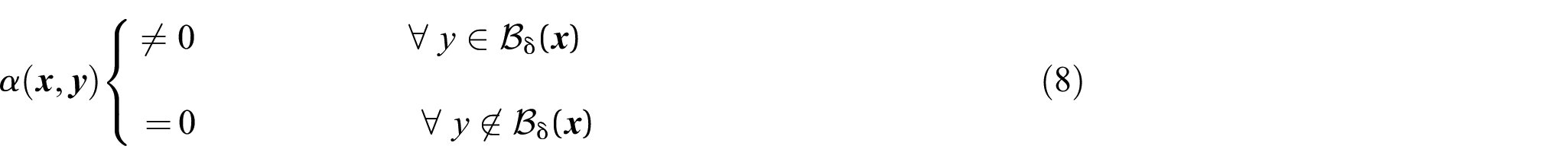
1. There is no self-interaction, i.e.,

2. The nonlocal action-reaction principle holds for

The action–reaction principle given by equation (3) simply states that the flux from
1.1.1. Nonlocal divergence and gradient operators and their adjoint
Given a vector two-point function

and

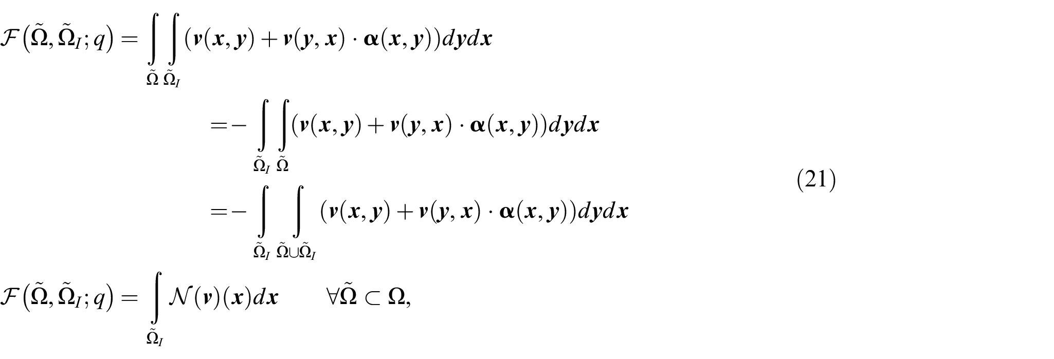
where
Given a scalar two-point function

and

Observe that, unlike in local calculus which deals with point functions only, nonlocal calculus involves two kinds of functions: point and two-point functions. This therefore necessitates the definition of alternative forms of the nonlocal operators defined in equations (4)–(7). The alternative forms of the nonlocal divergence and gradient operators were given in Galadima et al. [61] to be the pairs
1.1.2. Interaction kernels and domains
In equations (4)–(7), the two-point vector functions
Given two points
where

The interaction subdomain contains all the points
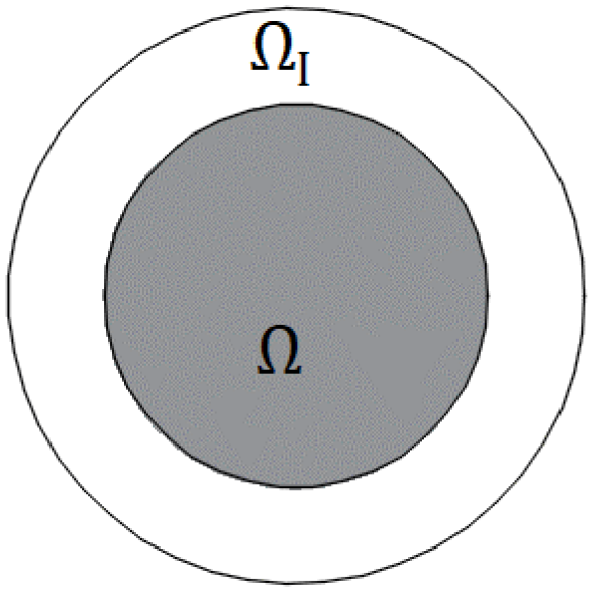
A typical relationship between
1.1.3. Nonlocal interaction operators
Given a domain

Corresponding to the nonlocal gradient operator

1.1.4. Nonlocal integral theorem
A very important outcome of the nonlocal operators developed in the proceeding subsections is statement of the nonlocal Gauss theorem. Recall from equation (2) that
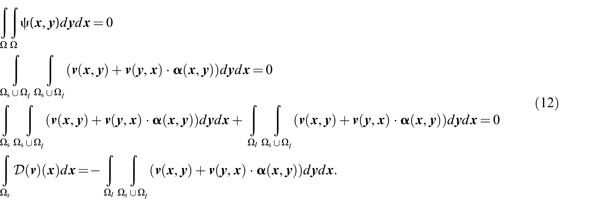

Consider the right-hand side of equation (12). If the interaction kernel function
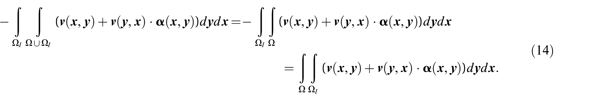
From equation (14) and considering equation (13), it can be deduced that
1.1.5. Nonlocal flux
From the statement of the divergence theorem which can be stated as the flux of a vector

1.2. Peridynamic model
The goal of the peridynamic theory is to provide a nonlocal alternative to the classical continuum theory that can unify the treatment of both continuous and discontinuous response of bodies in a single mathematical framework. Our goal in this section is to derive the nonlocal peridynamic transient heat conduction model using the principle of the nonlocal calculus presented in section 1.1. To proceed with our objective, it is necessary to restate some important concept in peridynamic theory. Given a bounded open domain

where
In the original development [1] that came to be known as the Bond-Based Peridynamics, interaction within a bond is independent of all other bonds. This lack of dependence imposes certain limitation to the peridynamic model. For example, in the realm of solid mechanics, this restricted the value of Poisson’s ratio to 1/3 for 2D and 1/4 for 3D isotropic solids. To circumvent this limitation and obtain a more general material model, State Based Peridynamics was developed. To pursue the development of the state based peridynamics, mathematical objects called states which are functions defined on bonds in

is the family of bonds for the point
1.2.1. The nonlocal peridynamic balance law
The governing equation of motion in PD can be formulated using the nonlocal vector calculus presented in section 1.1 based on a statement of balance law which postulate the dependence of the rate of change in the content of an extensive quantity over a given domain on the rate at which the quantity is produced within the domain and a flux through the boundary of the domain. Let the region occupied by a body

where equation (18) postulate that

If

If we write
where the third equality follows from consideration of equation (2) and the fourth is due to equation (10). The balance law equation (18) can now be written as

Applying the nonlocal divergence theorem equation (13) yields

which owing to the arbitrariness of

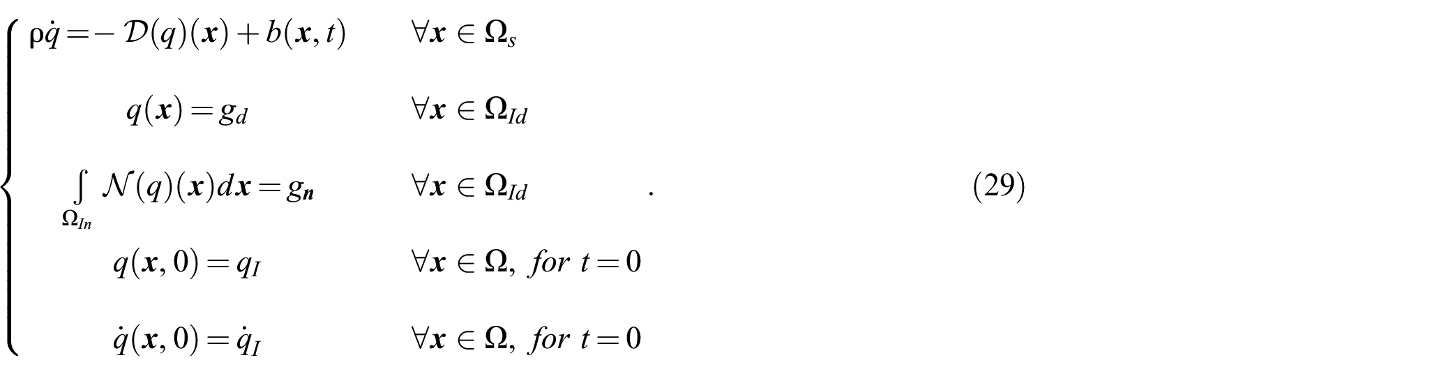
To uniquely determine

To prescribe the Neumann type constraint, recall that in the classical boundary value problem, this involves prescribing a flux density

The presence of the first order time derivative of the solution

and

are the initial conditions. So that equations (24)–(28) give the complete definition of the nonlocal problem which can be stated as
For the specific case of heat conduction,

where

The stored internal energy density

where
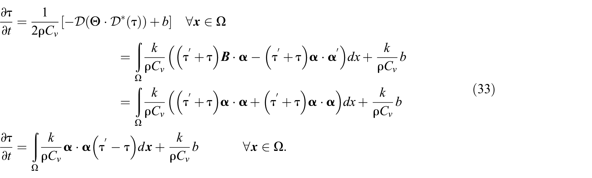
If we write

The integrand of the integral in equations (33) and (34) without the factor

where

Just like the micro-conductivity parameter, the micro-diffusivity function is also a parameter intrinsic to the material. Thus equation (34) can be written as

where
If we define the kernel function as

which leads to a form of the response function that appeared in Bobaru and Duangpanya [50] herein denoted as

If we, however, define

resulting in a response function that was proposed in Gerstle et al. [47] herein denoted as

On the other hand, if we define the kernel in equation (34) as

which corresponds to the form of the response function in previous works [62,67] given as

1.2.2. Relationship between micro-conductivity and thermal conductivity
The peridynamic micro-conductivity

where

where

The thermal potential from the classical model is given as

where
1.2.2.1. One-dimensional micro-conductivity
If a linear temperature field of the form

and equation (47) becomes

Let
where
Equating (49) and (51), respectively, yields

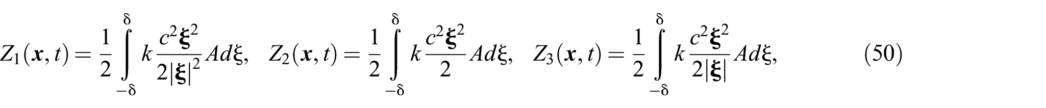
In the case where the distance between points is assumed to have considerable effect on the long-range thermal interaction between them, then the kernel function chosen for the micro-conductivity function must be able to capture the distribution of intensity of interaction. Typical kernel functions used in this case are the linear and quadratic kernel functions given, respectively, as

and

The micro-conductivity functions (equations (53)–(54)) all have compact support within the horizon. In other words, the interaction between a given point and any other point in a body cease if the distance between them is greater the horizon
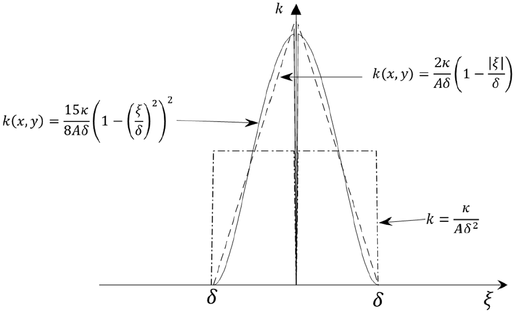
Comparison of micro-conductivity functions.
Although the different forms of the thermal response functions and their associated micro-conductivity functions have been established in the literature as cited, results of numerical experiments [67] have shown that the response function (equation (43)) provides the best approximation to the classical solution and would henceforth be used in the development of the proposed model reduction methodology. Also, the three different forms of the micro-conductivity functions presented in this section will be statically condensed in section 2.2. However, the choice of the micro-conductivity used in section 3 is limited to the constant function because of its simplicity of implementation and because the condensation of the peridynamic heat model with the other linear and quadratic micro-conductivity functions follows the same procedure.
1.2.2.2. Two-dimensional micro-conductivity function
Following the same procedure laid out in section 1.2.2.1, the explicit form of the constant and triangular micro-conductivity as well as the corresponding diffusivity modulus function can be obtained. A constant micro modulus function with its corresponding diffusivity function are given as

Interested readers are referred to Agwai [67] for discussion on the various forms of the response functions and their corresponding micro-conductivity functions.
1.2.3. The discrete heat conduction equation
Different discretization schemes have been proposed for the numerical approximation of balance laws arising from the peridynamic theory, such as the meshfree method [68,69], the collocation methods [70,71], and methods based on finite elements mesh [55,72]. Due to its simple implementation algorithm and relatively low computational cost, the meshfree method suggested in Silling and Askari [68] is the most widely used [73] and is the preferred method in this work for these same reasons. In this approximation method, the discrete form of equation (37) is

where
2. Static condensation of the peridynamic head conduction model
The assembled peridynamic transient heat conduction equations for the body in matrix form is given by

where

Neglecting the transient term and assuming there is no heat source at the truncated degrees of freedom, then the solution of the second submatrix equation for

where

The condensation matrix relates the retained degrees of freedom and truncated degrees of freedom and is load independent because it is assumed there is no heat source at the truncated degrees of freedom. Also note that in arriving at equation (59), the transient term in equation (58) has been neglected; hence, this method is called static condensation method. The temperature state of the full model may be expressed as

where

where

Substituting equations (62) and (63) into equation (57) and pre-multiplying by

where

2.1. Handling boundary conditions
It is necessary to provide some notes on how the Dirichlet and Neumann boundary conditions are handled in this model order reduction scheme. When implementing the static condensation procedure, the region constrained by a Dirichlet type boundary condition must be retained in the reduced model. This is because in Dirichlet boundary condition, a specified value of the temperature is imposed on the boundary volume. As can be seen from equation (8), there is no transformation on the temperature field. Hence, to preserve the dynamics of the system, any boundary with Dirichlet condition imposed must be retained. This is not the case with Neumann boundary condition. This is because in Neuman type boundary condition, instead of temperature, a specified value of heat is applied to the boundary volume. From equation (8) and the definitions in equation (9), in going from the full model to a reduced model, there is a transformation relation between the heat source term in the full model and its counterpart in the reduced model (see the third definition in equation (9)). Therefore, irrespective of what region is retained in the reduced model, the characteristics of the full model are preserved. This affords more flexibility on the final configuration of the reduced model compared with the Dirichlet boundary condition scenario.
2.2. Condensation of parameters of peridynamic heat conduction model
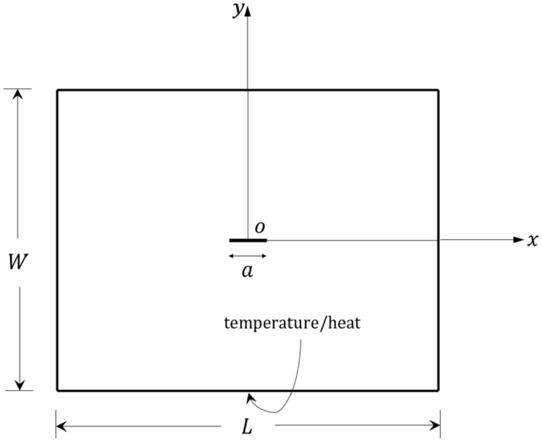
The condensation of the micro-conductivity and micro-diffusivity functions will be illustrated using an example of a bar as shown in Figure 3. The goal is to demonstrate the behaviour of the peridynamic parameters when subjected to static condensation. Let the bar be of length
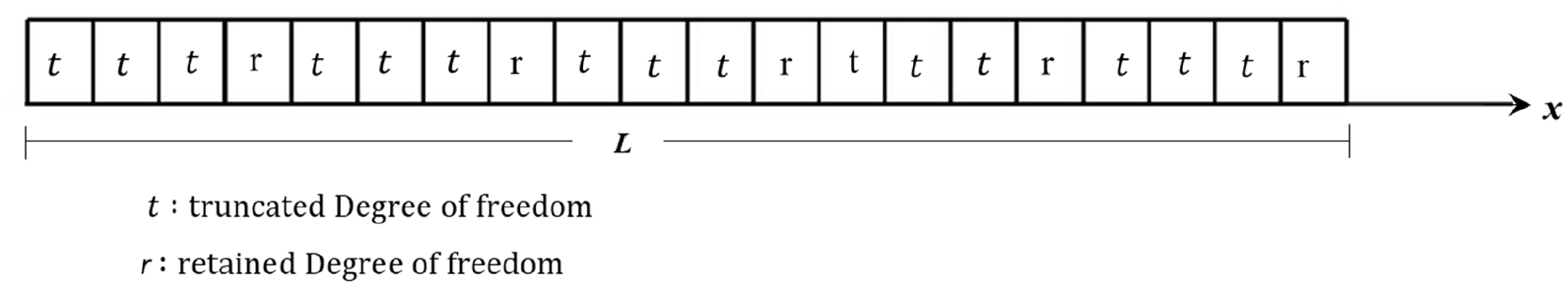
A discretized bar to illustrate condensation of the micro-conductivity functions.
The horizon is
The condensed curves of the micro-conductivity functions and the micro-diffusivity functions are characterized by sharp spikes as can be seen from Figures 4 and 5, respectively. This behaviour is expected since the condensed model is defined only at the retained degrees of freedom.
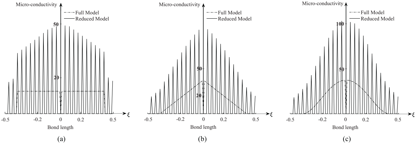
Static condensation of micro-conductivity functions of a homogeneous bar: (a) constant micro-conductivity, (b) linear micro-conductivity, and (c) quadratic micro-conductivity.
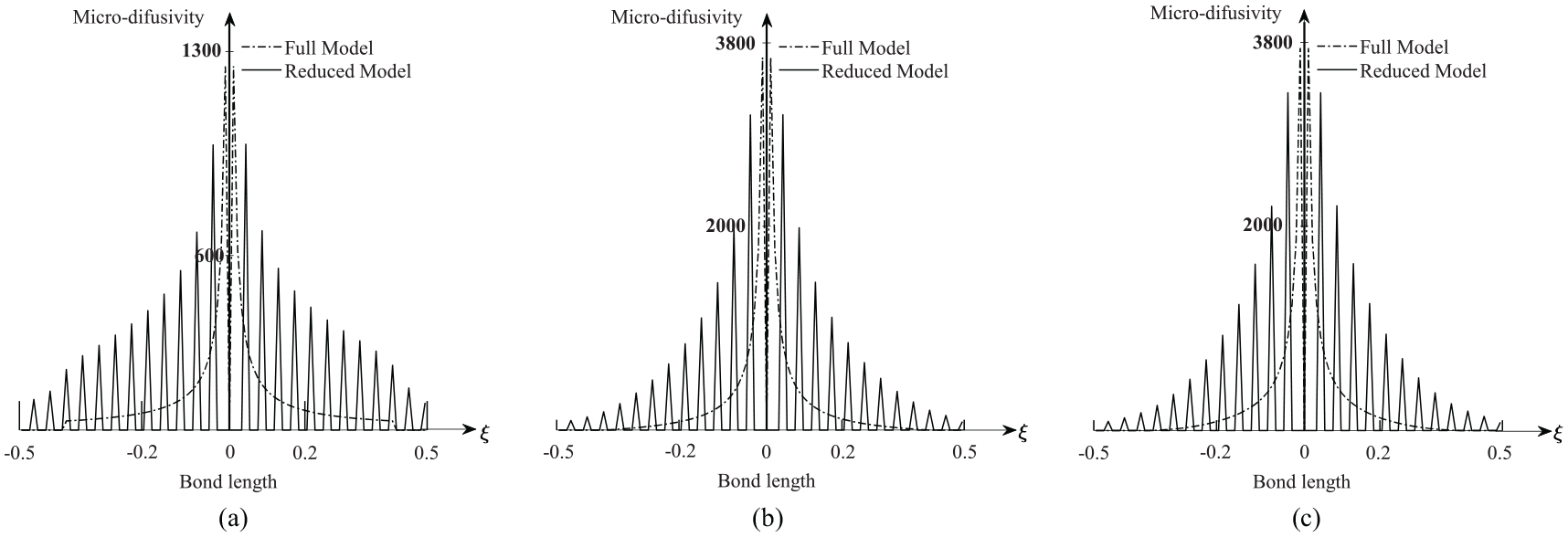
Static condensation of micro-diffusivity functions of a homogeneous bar: (a) corresponding to constant micro-conductivity, (b) corresponding to linear micro-conductivity, and (c) corresponding to quadratic micro-conductivity.
3. Numerical verification
The static condensation scheme described in section 2 will be tested on numerical problems to verify and demonstrate its capabilities in reducing the order of a peridynamic transient heat conduction model. To achieve this goal, the temperature field in a one-dimensional bar and two-dimensional plate is predicted using the proposed static condensation scheme and the result is compared with prediction using the full model.
3.1. A homogeneous bar with constant temperature applied at both ends
A homogeneous bar initially at zero temperature is subjected to boundary temperature of 1°C at both ends as shown in Figure 6. The bar has a length and thickness of 1 m and 0.01 m, respectively. The specific heat capacity, thermal conductivity, and density of the bar are specified as
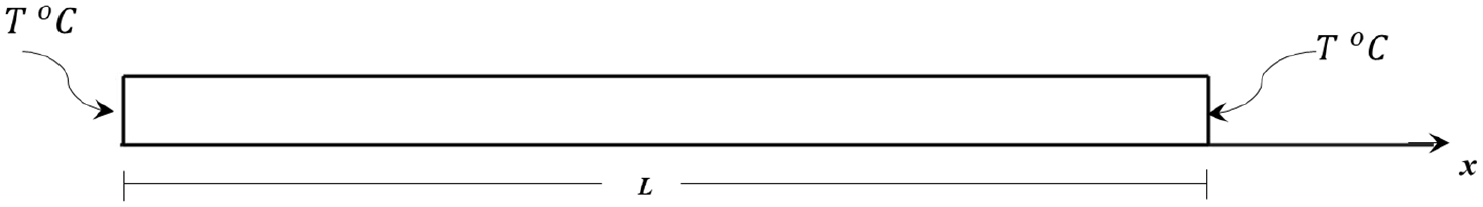
A homogeneous bar subjected to constant temperature at both ends.
The bar is discretized into
Temperature prediction for both full model and reduced model for the three instances of reduction are presented in Figures 7–9. The reported results are temperature distribution across the bar corresponding to time steps
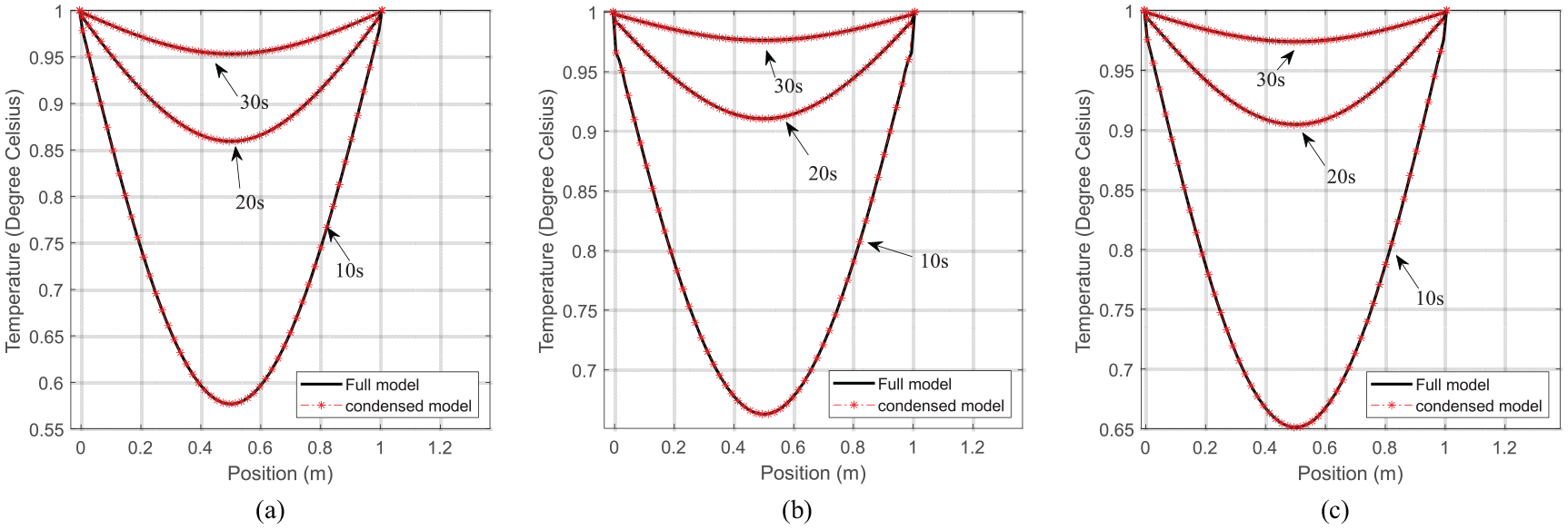
Temperature distribution in a homogeneous bar subjected to constant temperature at both ends corresponding to retaining every second node of the full model and response function (a)
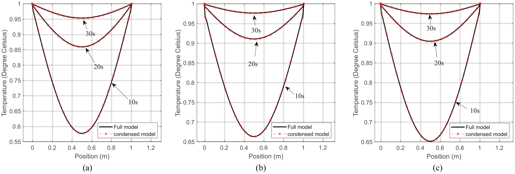
Temperature distribution in a homogeneous bar subjected to constant temperature at both ends corresponding to retaining every fifth node of the full model and response function (a)
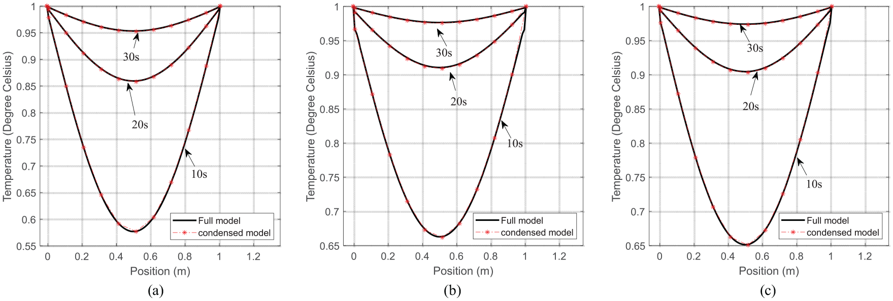
Temperature distribution in a homogeneous bar subjected to constant temperature at both ends corresponding to retaining every 10th node of the full model and response function (a)
3.2. Numerical study of heat conduction in plate with a pre-existing crack
The static condensation scheme will be used to study temperature distribution in a plate with a pre-existing crack. The geometry of the plate is specified as length
Example 2 problem setup: A plate with pre-existing crack.
The numerical implementation of the peridynamic transient heat conduction model proceed by discretizing the plate into
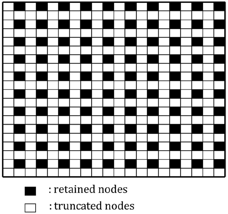
Schematic representation of static condensation.
3.2.1. Example 1. Case I: Dirichlet boundary condition
In this case, the plate is subjected to the following initial and boundary conditions, respectively:

and

Note that in this case, although the condensation algorithm may exclude the boundary nodes, we are constrained to still retain them. Temperature distribution in time across the plate for both full model and the reduced model are shown Figure 12. A profile of the temperature along a grid of nodes parallel to the vertical axis of the plate at
Dirichlet boundary condition: Temperature distribution across the plate: (a) Full model corresponding to
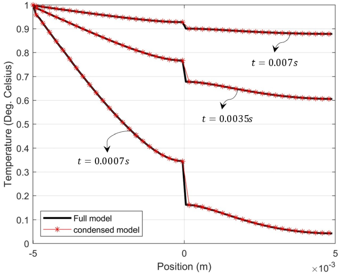
Temperature profile along the grid at
The results presented in Figures 12 and 13 show a very good match between predictions from the full model and those from the reduced model. The difference between the full model and reduce model curves close to the crack location in Figure 13 reflects wider spacing between nodes in the reduced model due to fewer nodes. Note that all boundary nodes subjected to the Dirichlet boundary condition were retained in the reduced model.
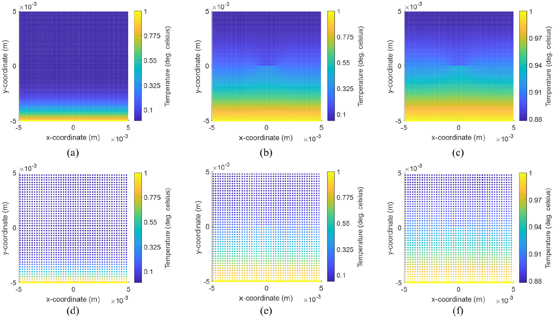
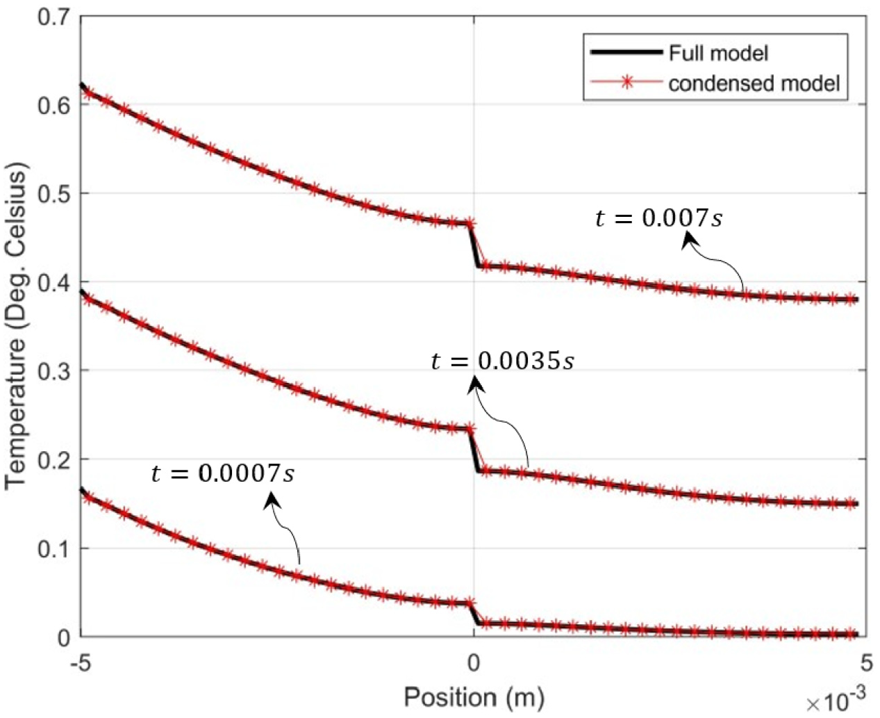
3.2.2. Example 2. Case II: Neumann boundary condition
The goal in this example is to demonstrate the performance of the model order reduction in reducing a 2D model with a Neumann type boundary condition. In this case, in addition to equation (66), the plate is subjected to the following conditions:

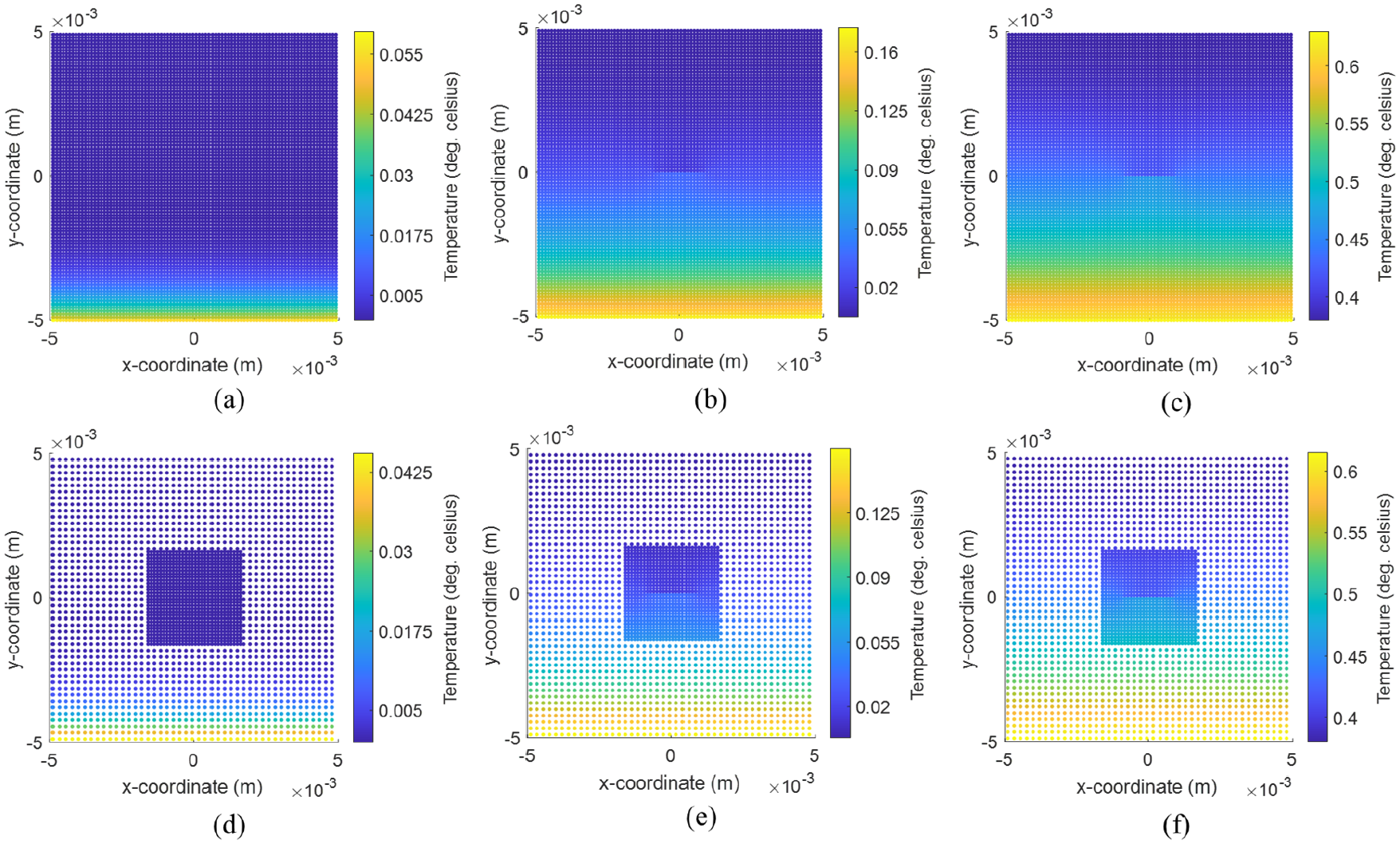
Figure 14(a)–(c) illustrates the full model prediction of the distribution of temperature over the plate, while Figure 14(d)–(f) are the predicted temperature distribution in the plate from the reduced model corresponding to simulation times

Neumann boundary condition: Temperature distribution across the plate: (a) Full model corresponding to
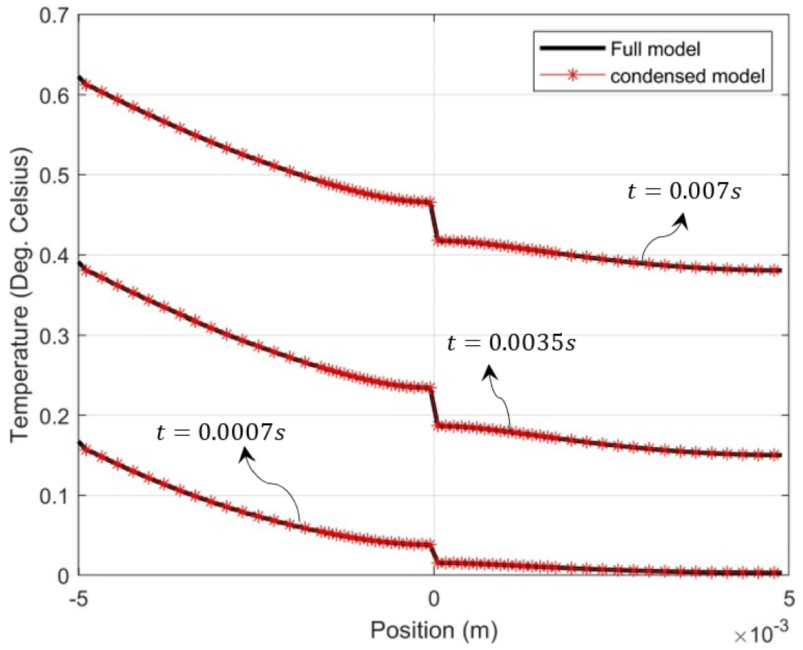
Temperature profile along the grid at
The results presented show a near identical match between predictions from the full model and those from the reduced model. It is worthy to note that in the case of the Neumann type boundary condition, there was no constraint to the choice of nodes to retain and those to be condensed out. This potentially allows for the use of fewer degrees of freedom than in the scenario where a Dirichlet type boundary condition is imposed.
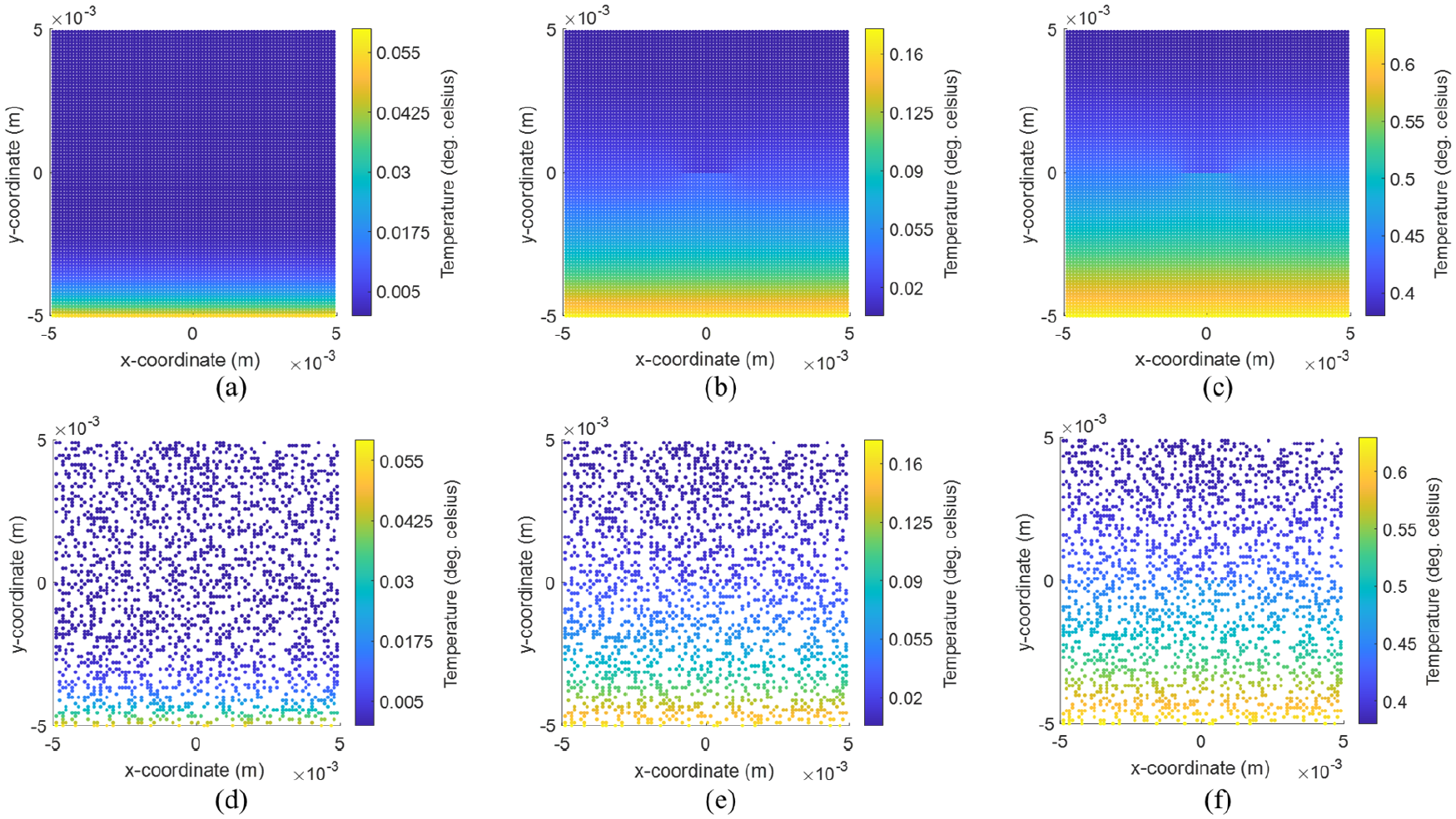
3.2.3. Example 3. Neumann boundary condition with retained nodes selected randomly
In this example, the plate of example 2 will be analysed using the same boundary conditions and plate properties. However, in coarsening the plate, instead of following a predetermined pattern as done in the previous examples, the retained nodes in this case will be selected randomly. The goal is to demonstrate the robustness of the condensation methodology in handling any kind of selection pattern during model reduction. In this condensation scheme, 2,025 nodes were randomly selected from a total of 8,190 nodes. Result of the temperature distribution over the surface of the plate is shown in Figure 16, while the temperature profile of nodes that falls along a grid located at
Neumann boundary condition: Temperature distribution across the plate: (a) Full model corresponding tot = 7×10^(-5) s, (b) Full model corresponding to t = 7×10^(-4) s (c) Full model corresponding to t = 7×10^(-3) s,(d) Reduced model corresponding.
The results presented in Figures 16 and 17 show good agreement between prediction from the full model and the condensed model. This is a demonstration of the robustness of the condensation methodology in predicting accurate result irrespective of the algorithm or pattern employed in the condensation process.
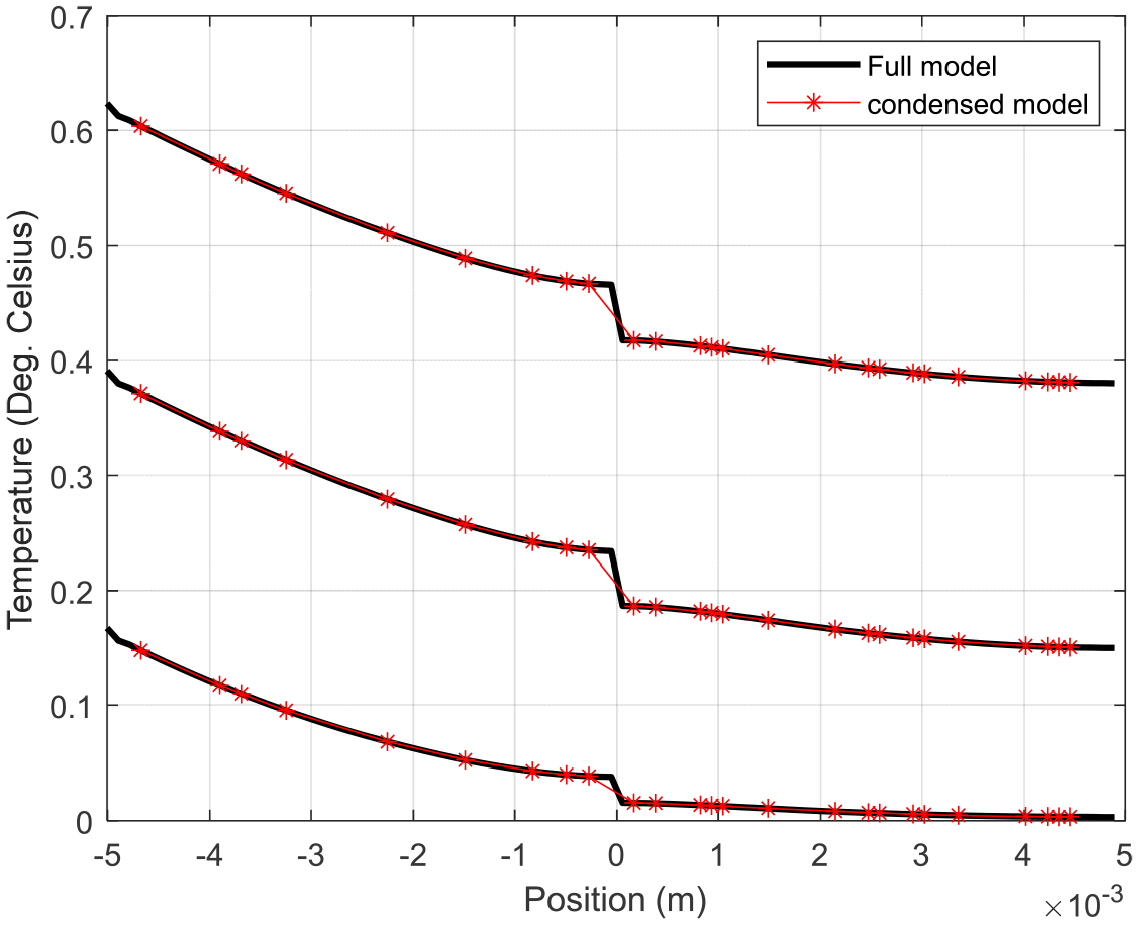
Temperature profile along a grid of the plate with Neumann boundary condition and condensation achieved through random selection of nodes.
3.2.4. Example 3. Nonuniform condensation
It is sometimes necessary to have high resolution at certain region of the model while such level of detail may not be required in other regions. This model order reduction can be selectively applied to accommodate this different resolution requirement. For example, high resolution may be required around regions close to the crack of the plate in section 3.2.2 to allow for more detailed information than is required in regions further away from the cracks. To achieve this, a nonuniform condensation algorithm will be implemented in this example where all nodes around the crack are retained and regions further away from the crack will be condensed. The region around the crack is defined by a square of dimension
Prediction of temperature distribution in time using the adaptive condensation scheme is presented alongside prediction from the full model in Figure 18. Temperature profile along a grid of nodes parallel to the vertical axis is also presented in Figure 19. In addition to the near identical prediction from both models as can be seen from Figures 18 and 19, the temperature profile near the crack for both curves are also near identical. This contrasts with the case in sections 3.2.1 and 3.2.2 where there is a slight difference between the curves from the full and reduced models.
Adaptive condensation: Temperature distribution across the plate: (a) Full model corresponding to
Adaptive condensation. Temperature profile along a grid of the plate with Neumann boundary condition.
4. Conclusion
In this paper, we have been able to utilize a nonlocal vector calculus to derive the general form of the nonlocal peridynamic transient heat conduction equation. Using specific kernel functions, we show how the different explicit forms of the peridynamic heat transport equation developed in the literature can be recovered from the general form.
A model order reduction of the nonlocal peridynamic transient heat conduction model based on static condensation algorithm was implemented. The results from predictions based on the full order model and reduced order model show a near perfect match, thus demonstrating the capability of the model reduction scheme in preserving the characteristics of the system. The model reduction scheme also allows for adaptive implementation of the condensation algorithm so that a more detailed model is implemented in regions where higher resolution results are needed for greater insight into the numerical predictions.
The development in this study only treats systems with time invariant physical and geometrical characteristics. For example, model parameters such as the thermal conductivity or peridynamic bonds existing between material points must be time invariant. Because of this constraint, treatment of thermal conduction problems in the presence of propagating cracks is beyond the capabilities of the present scheme. In a future endeavour, the authors would like to extend the capabilities of this model order reduction scheme to problems with time dependent properties.
Footnotes
Funding
The author(s) disclosed receipt of the following financial support for the research, authorship, and/or publication of this article: The first author is supported by the government of the federal republic of Nigeria through the Petroleum Technology Development Fund (PTDF). This material is based upon work supported by the Air Force Office of Scientific Research under award number FA9550-18-1-7004.