Model order reduction of linear peridynamic systems using static condensation

Abstract

Static condensation is widely used as a model order reduction technique to reduce the computational effort and complexity of classical continuum-based computational models, such as finite-element models. Peridynamic theory is a nonlocal theory developed primarily to overcome the shortcoming of classical continuum-based models in handling discontinuous system responses. In this study, a model order reduction algorithm is developed based on the static condensation technique to reduce the order of peridynamic models. Numerical examples are considered to demonstrate the robustness of the proposed reduction algorithm in reproducing the static and dynamic response and the eigenresponse of the full peridynamic models.

1. Introduction

The increasing requirement for cost saving means that more complex and increasingly larger systems need to be mathematically modelled and simulated, thus increasing computational time and cost. To ensure computational efficiency, various techniques have been developed to reduce the size of the model to be solved for either static or dynamic responses.

Every mathematical model is an attempt to imitate a physical process. Because of the uncertainties involved in the parameters that describe the system, such as loads and material properties, inaccuracies are inevitably introduced into the model and ultimately to the predicted response of the system. In the design of high-technology systems, the accuracy of the mathematical model is crucial because the margin for errors for such systems is usually much smaller than for conventional systems. It therefore becomes necessary to verify results obtained from virtual simulation with experimental results.

Traditionally, finite-element models are used to predict the static and dynamic responses of structural systems across a wide spectrum of industries, such as aerospace, automobile and civil engineering. Where the mathematically predicted dynamic response of the system needs to be verified experimentally, a structural dynamic test is conducted on a physical model. Usually, the dynamic experiment is conducted with fewer degrees of freedom (DoFs) than the mathematical model. This represents a classic motivation to develop model reduction techniques, the objective of which is to allow for correlation of the dynamic response from experiment with that of the mathematical model by reducing the DoFs of the finite-element model in order to eliminate the problem of mesh incompatibility. The reduced mathematical model in this sense is called a test analysis model [1]. Several techniques have been proposed to help with the condensation of static and dynamic finite-element models [2–7].

Despite its many successes, there are still numerous problems for which the finite-element method based on the classical continuum model is simply inadequate. One factor responsible for the inadequacy is the fact that the governing equations describing the response of systems in the classical continuum theory rely on spatial derivatives. Such partial derivatives, by their nature, are not valid in the presence of discontinuous system responses, such as cracks.

Peridynamic theory was primarily developed [8] to overcome the shortcomings of the classical continuum mechanics in handling discontinuous system responses. Built on a mathematical framework based on an integro-differential framework, the development of peridynamic theory paved the way for unification of the mathematical modelling of continuous media, fractures and particles in a single modelling framework, which can find application in situations involving evolution and propagation of discontinuities, such as crack nucleation and growth, using the same field equation as in the continuous case. Another feature of the peridynamic formulation is that it is a nonlocal theory that incorporate the concept of long-range force by allowing interaction of particles located at finite distance from each other through a pairwise force field.

Since its introduction [8], peridynamic theory has been successfully deployed to study a range of engineering systems [9–15]. However, the use of peridynamic theory in solving practical engineering problems implies dealing with systems with very large DoFs. This comes with the attendant consequence of high computational cost. In response, several multiscale techniques have been proposed to achieve the goal of reducing complexity of peridynamic models. An adaptive refinement and multiscale algorithm was developed [16], which essentially allowed use of variable horizon sizes in different regions of a peridynamic model to gain computational efficiency.

A hierarchical multiscale modelling framework that coupled molecular dynamics with peridynamics was developed [17]. The coupling of peridynamic particles at coarse scale and fine-scale molecular dynamics particles was achieved through an intermediate mesoscale model called the coarse-grain atomic model. The algorithm so developed was a hierarchical downscaling framework that allowed information about the system at the peridynamic macroscale to be transferred and captured at the molecular dynamics microscale.

A coarsening method for linear peridynamics was proposed and implemented for one dimension [18] and was extended [19] for two-dimensional applications. The objective of the coarsening algorithm was to derive a simplified model from a detailed and more complex model by retaining fewer DoFs, on the one hand, and preserving the effect of the excluded DoFs in the response of the model, on the other hand. Numerical investigation conducted in both works [18, 19] demonstrated the robustness of the technique in reducing the order of the peridynamic model for a range of problems, without compromising on predictive capability.

A key limitation of the coarsening algorithm is the fact that the boundary data must be specified on the retained DoFs. In other words, the applied body force or prescribed nonzero displacement must be specified on the retained DoFs. This consequently places restrictions on which DoFs to eliminate and which to retain. Another limitation of the coarsening method is that the algorithm is not suitable for application in solving dynamic equilibrium problems.

The objective in this work is to present a model order reduction algorithm based on a static condensation method [2] that is similar to the coarsening methodology [18] described in that both methodologies seek to reduce the complexity of a peridynamic model and hence computational effort by reducing the DoFs of the model and yet are still able to accurately predict the response of the system. However, the proposed algorithm in this work promises to provide extended capabilities covering both static and dynamic system responses. Numerical investigation will be conducted to demonstrate the robustness of the algorithm in effectively reducing the order of peridynamic models for static, dynamic and modal responses.

In what will follow, a brief overview of the peridynamic theory will be given in Section 2, while the algorithm and procedure of statically condensing a peridynamic model will be laid out in Section 3. In Section 3.1, the expression for static condensation of the peridynamic static response problem will be derived, to be followed in Section 3.2 by the derivation of the expression for the static condensation of the peridynamic dynamic response analysis. In Section 3.3, the modal equations of peridynamic theory will be derived, and the proposed condensation algorithm will be applied to obtain the reduced-order model for the peridynamic eigenproblem. The general form of the reduced micromodulus function is presented in Section 4. A numerical demonstration of the capabilities of the proposed reduction algorithm in reproducing the static, dynamic and modal responses of the peridynamic model using fewer DoFs is presented in Section 5.

2. Peridynamic theory

Recalling from the classical continuum theory, the equation of motion of a medium arising from conservation of momentum is

$$\rho \left(x\right)\stackrel{··}{u}(x,t)=\nabla ·\sigma +b(x,t)$$

(1)

where ρ is the mass density of the medium, σ is the stress tensor, b is a vector of body force density, $\stackrel{··}{u}$ is the acceleration vector field and x is a vector that represents the location of material points (particles) within the medium at time t. The key challenge in using equation (1) to model discontinuous system behaviour is the presence of the gradient operator, which implies the existence of the spatial derivative of the stress field and consequently the displacement field within the domain of interest. However, since these field variables are not continuous over such features as crack tips and crack surfaces, the derivatives in such instances are undefined. In the peridynamic formulation, the equation of motion was cast such that the integral operators replaced the derivatives on the right-hand side of equation (1). A ‘bond-based’ peridynamic equation of motion was originally proposed [8] as

$$\rho \left(x\right)\stackrel{··}{u}(x,t)=\underset{{\mathcal{H}}_x}{\int }\mathbf{f}(u(q,t)-u(x,t),q-x)\mathrm{d}{V}_q+b(x,t),$$

(2)

where u is the displacement vector field and ${\mathcal{H}}_x$ is the neighbourhood (horizon) of the particle located at point x. The pairwise force function f is the force per unit volume squared that a particle located at point q exerts on a particle located at point x.

If we assume a linear material behaviour, the pairwise force function [8] takes the form

$$\mathbf{f}(\eta ,\xi )=C\left(\xi \right)\eta ,\forall \xi ,\eta ,$$

(3)

where $C\left(\xi \right)$ is a tensor-valued function called the micromodulus function, given by

$$\mathrm{C}\left(\xi \right)=\frac{\partial f(0,\xi )}{\partial \eta },\forall \xi .$$

(4)

The peridynamic equation of motion (equation (2)) therefore specialises to

$$\rho \left(x\right)\stackrel{··}{u}(x,t)=\underset{{\mathcal{H}}_x}{\int }C(x,q)(u(q,t)-u(x,t))\mathrm{d}{V}_k+b(x,t)$$

(5)

The discretised form of equation (5), as described in [13], is

$$\rho {\stackrel{··}{u}}_i^n=\sum _j^{N_i}C(x_j-x_i)(u_j-u_i)V_j+b_i^n,$$

(6)

where N_i is the number of particles within the horizon of the particle located at x_i. The assembled peridynamic equations of equilibrium for the body in matrix notation take the form

$$\left[M\right]\left\{\stackrel{··}{u}\right\}+\left[C\right]\left\{u\right\}=\left\{b\right\},$$

(7)

where {u} is a vector of all displacement DoFs, {b} is a vector that collects all applied body forces, [M] is a diagonal matrix of mass density and [C] is the micromodulus matrix, which is analogous to the stiffness matrix in the finite-element method.

3. Static condensation

3.1. Reduced static peridynamic models

Consider a linear peridynamic body $\mathcal{B}$ that is discretised into N material points. Considering a static response, the equation of motion (equation (7)) for a system of N material points is

$${\left[C\right]}_{N\times N}{\left\{u\right\}}_N={\left\{b\right\}}_N.$$

(8)

The objective is to replace this system with a reduced DoF system while maintaining the kinematic characteristics of the original system. Let $\left\{u_a\right\}\subset {\left\{u\right\}}_N$ be the primary (active) DoFs to be retained and $\left\{u_d\right\}\subset {\left\{u\right\}}_N$ be the secondary DoFs to be condensed out.

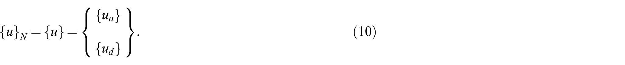
In the condensation process, the assembled peridynamic equilibrium equations are partitioned, as

$$\left[\begin{array}{cc}\left[C_{\mathrm{aa}}\right]\hfill & \left[C_{\mathrm{ad}}\right]\hfill \\ \multicolumn{1}{c}{\left[C_{\mathrm{da}}\right]}& \left[C_{\mathrm{dd}}\right]\hfill \end{array}\right]\left\{\begin{array}{c}\left\{u_a\right\}\hfill \\ \multicolumn{1}{c}{\left\{u_d\right\}}\end{array}\right\}=\left\{\begin{array}{c}\left\{b_a\right\}\hfill \\ \multicolumn{1}{c}{\left\{b_d\right\}}\end{array}\right\}.$$

(9)

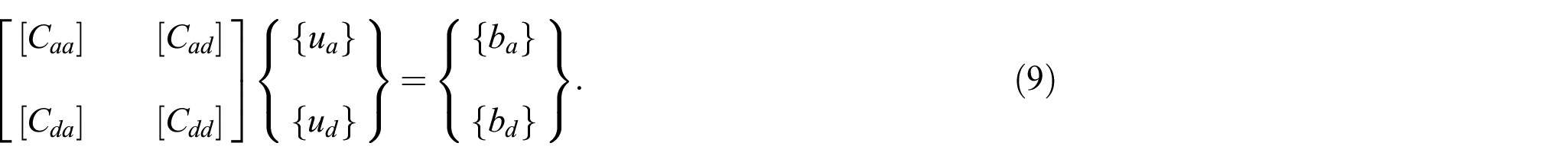
The global vector of DoFs of the system may be written as

$${\left\{u\right\}}_N=\left\{u\right\}=\left\{\begin{array}{c}\left\{u_a\right\}\hfill \\ \multicolumn{1}{c}{\left\{u_d\right\}}\end{array}\right\}.$$

(10)

Multiplying out equation (9), we have

$$\left[C_{\mathrm{aa}}\right]\left\{u_a\right\}+\left[C_{\mathrm{ad}}\right]\left\{u_d\right\}=\left\{b_a\right\},$$

(11)

$$\left[C_{\mathrm{da}}\right]\left\{u_a\right\}+\left[C_{\mathrm{dd}}\right]\left\{u_d\right\}=\left\{b_d\right\}.$$

(12)

Consider the solution to equation (12). If $\left[C_{\mathrm{dd}}\right]$ is nonsingular, we can solve for the DoFs to be condensed out:

$$\left\{u_d\right\}={\left[C_{\mathrm{dd}}\right]}^{-1}(\left\{b_d\right\}-\left[C_{\mathrm{da}}\right]\left\{u_a\right\}).$$

(13)

Substituting equation (13) into equation (11) yields

$$\left[C_G\right]\left\{u_a\right\}=\left\{b_G\right\}.$$

(14)

Equation (14) is the condensed linearised peridynamic equilibrium equation, where

$$\left[C_G\right]=\left[C_{\mathrm{aa}}\right]-\left[C_{\mathrm{ad}}\right]{\left[C_{\mathrm{dd}}\right]}^{-1}\left[C_{\mathrm{da}}\right],\left\{b_G\right\}=\left\{b_a\right\}-\left[C_{\mathrm{ad}}\right]{\left[C_{\mathrm{dd}}\right]}^{-1}\left\{b_d\right\}$$

(15)

are the condensed micromodulus matrix and the body force vector, respectively. If we assume the inertia contribution as well as the external forces acting on the secondary DoFs to be negligible, this will permit a static relationship between the primary DoFs and the secondary DoFs such that equation (12) yields

$$\left\{u_d\right\}=\left[R_G\right]\left\{u_a\right\},$$

(16)

where $\left[R_G\right]\in R^{d\times a}$ represents the Guyan condensation matrix, which is defined as

$$\left[R_G\right]=-{\left[C_{\mathrm{dd}}\right]}^{-1}\left[C_{\mathrm{da}}\right].$$

(17)

Introducing equation (17) into equation (10) gives the expression

$$\left\{u\right\}=\left[T_G\right]\left\{u_a\right\}.$$

(18)

In equation (18), $\left[T_G\right]\in R^{n\times a}$ is a linear transformation matrix that maps DoFs in the reduced model onto DoFs in the full model and is defined as

$$\left[T_G\right]=\left[\begin{array}{c}\left[\mathrm{I}\right]\hfill \\ \multicolumn{1}{c}{\left[R_G\right]}\end{array}\right],$$

(19)

where [I] is an $a\times a$ identity matrix. It is easily verifiable that equation (15) can be expressed as

$$\left[C_G\right]={\left[T_G\right]}^{\mathrm{T}}\left[C\right]\left[T_G\right],\left\{b_G\right\}={\left[T_G\right]}^{\mathrm{T}}\left\{b\right\}.$$

(20)

Note that the static condensation is so called because we ignored the inertia effect on the deleted DoFs. Also note that in order to obtain the expression for the transformation matrix in equation (19), an assumption of zero body force density acting on the deleted DoFs was made. However, the fact that the expansion of equation (20) exactly gives the expression in equation (15) shows that this assumption does not affect the reduced stiffness matrix and the reduced force density vector. The condensed peridynamic equilibrium equations as represented by equation (14) yields the exact solution of the peridynamic model at the retained material points, as would be obtained if we used the detailed model.

3.2. Reduced dynamic models

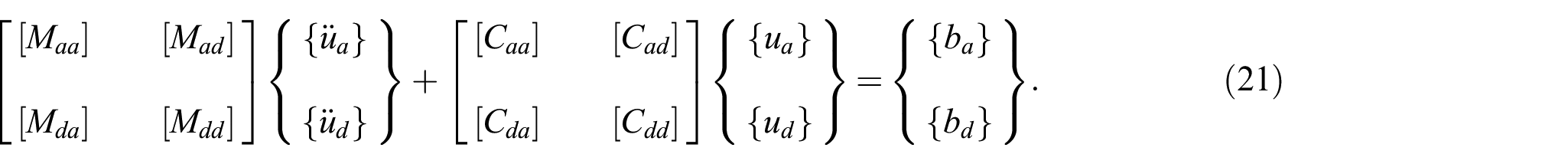
To reduce the order of a dynamic peridynamic model, the equation of motion given in equation (7) may be written in partitioned form:

$$\left[\begin{array}{cc}\left[M_{\mathrm{aa}}\right]\hfill & \left[M_{\mathrm{ad}}\right]\hfill \\ \multicolumn{1}{c}{\left[M_{\mathrm{da}}\right]}& \left[M_{\mathrm{dd}}\right]\hfill \end{array}\right]\left\{\begin{array}{c}\left\{{\stackrel{··}{u}}_a\right\}\hfill \\ \multicolumn{1}{c}{\left\{{\stackrel{··}{u}}_d\right\}}\end{array}\right\}+\left[\begin{array}{cc}\left[C_{\mathrm{aa}}\right]\hfill & \left[C_{\mathrm{ad}}\right]\hfill \\ \multicolumn{1}{c}{\left[C_{\mathrm{da}}\right]}& \left[C_{\mathrm{dd}}\right]\hfill \end{array}\right]\left\{\begin{array}{c}\left\{u_a\right\}\hfill \\ \multicolumn{1}{c}{\left\{u_d\right\}}\end{array}\right\}=\left\{\begin{array}{c}\left\{b_a\right\}\hfill \\ \multicolumn{1}{c}{\left\{b_d\right\}}\end{array}\right\}.$$

(21)

If we assume the micromodulus function $\left[C\right]$ to be time-invariant, then $[T_G]$ is independent of time and hence the second derivative of equation (18) with respect to time yields

$$\left\{\stackrel{··}{u}\right\}=\left[T_G\right]\left\{{\stackrel{··}{u}}_a\right\}.$$

(22)

Introducing equations (18) and (22) into equation (7) and premultiplying both sides by the transpose of the transformation matrix $\left[T_G\right]$ gives the equation of equilibrium of the reduced model:

$$\left[M_G\right]\left\{{\stackrel{··}{u}}_a\right\}+\left[C_G\right]\left\{u_a\right\}=\left\{b_G\right\},$$

(23)

where the matrices $\left[M_G\right]$ and $\left[C_G\right]$ and the vector $\left\{b_G\right\}$ are the condensed mass matrix, condensed micromodulus matrix and condensed body force vector, respectively, associated with the reduced model, defined as

$$\left[M_G\right]={\left[T_G\right]}^{\mathrm{T}}\left[M\right]\left[T_G\right],\left[C_G\right]={\left[T_G\right]}^{\mathrm{T}}\left[C\right]\left[T_G\right],\left\{b_G\right\}={\left[T_G\right]}^{\mathrm{T}}\left\{b\right\},$$

(24)

If we neglect dynamic effects in the reduced model, equation (23) specialises to the reduced model for the static problem defined in equation (14). Since the majority of storage requirement and computational effort required to implement this condensation technique is used in the computation of ${\left[C_{\mathrm{dd}}\right]}^{-1}$ , a computationally more efficient way to achieve the condensation of the peridynamic static model is to employ the standard Gauss–Jordan elimination procedure [20].

3.3. Reduced eigenvalue models

Assume that the solution u to equation (5) is given by the general form of a plane wave:

$$u(x,t)=A{e}^{\mathrm{i}(\mathrm{kx}-\omega t)},$$

(25)

where u is the displacement of a point x, A is the constant amplitude vector, k is the wave number, $\omega$ is the wave frequency and t is time. Substituting equation (25) into equation (5) and assuming no body force applied will yield

$$-{\omega }^2\rho \left(x\right)A=\underset{{\mathcal{H}}_x}{\int }C(x,q)({\mathrm{e}}^{\mathrm{i}k(q-x)}-1)d{V}_k·A.$$

(26)

Taking Euler’s transformation of equation (26) gives

$$-{\omega }^2\rho \left(x\right)u(x,t)=\underset{{\mathcal{H}}_x}{\int }C(x,q)(\cos \left(k(q-x)\right)+\mathrm{i}\sin \left(k(q-x)\right)-1)d{V}_k·u(x,t).$$

(27)

Since the micromodulus function is an even function and $\sin \left(k(q-x)\right)$ is an odd function, equation (27) reduces to

$${\omega }^2\rho \left(x\right)A=\underset{{\mathcal{H}}_x}{\int }C(x,q)(1-\cos \left(k(q-x)\right))d{V}_k·A.$$

(28)

It can be inferred from equation (4) that the integral in equation (28) can be written in a matrix form. Using the simplified notation

$$\mathcal{D}(k,\xi )=\underset{{\mathcal{H}}_x}{\int }C(x,q)(1-\cos \left(k(q-x)\right))d{V}_k$$

(29)

with the definition that $\xi =q-x$ , equation (29) can be written as

$${\omega }^2\rho \left(x\right)A=\mathcal{D}(k,\xi )·A,$$

(30)

which gives us a classical eigenvalue problem with the following characteristic equation:

$$|\mathcal{D}(k,\xi )-{\omega }^2\rho \left(x\right)|=0.$$

(31)

The dispersion matrix $\mathcal{D}(k,\xi )$ first appeared in [8]. The eigenvalues and eigenvectors resulting from equation (31) give the natural frequencies and natural modes of the peridynamic system. Equation (31) may be written in matrix form as

$$|\left[\mathcal{D}\right]-{\omega }^2\left[M\right]|=0.$$

(32)

In equation (32), $\left[M\right]=\rho \left[\mathrm{I}\right]$ is the mass-density matrix and $\left[\mathrm{I}\right]$ is the identity matrix. The reduced-order eigenvalue problem may be stated as

$$|\left[{\mathcal{D}}_G\right]-{\omega }^2\left[M_G\right]|=0,$$

(33)

where $\left[{\mathcal{D}}_G\right]$ is the statically condensed dispersion matrix, and is defined as

$$\left[{\mathcal{D}}_G\right]={\left[T_G\right]}^{\mathrm{T}}\left[\mathcal{D}\right]\left[T_G\right].$$

(34)

4. Condensation of the micromodulus function

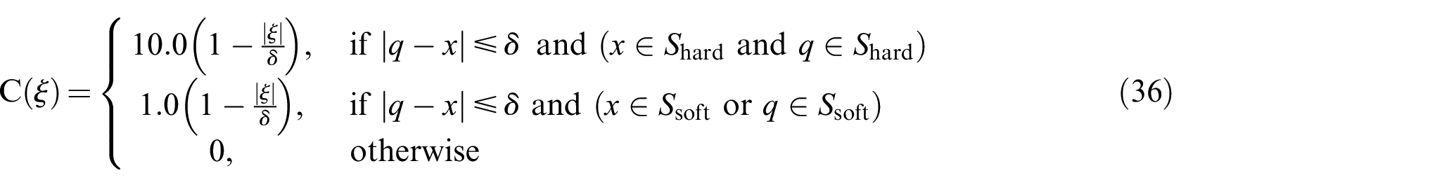
This section will illustrate the typical form of a condensed micromodulus function. Consider a one-dimensional homogeneous bar of length 1.0 with a micromodulus function of the form

$$\mathrm{C}\left(\xi \right)=\{\begin{array}{cc}1.0(1-\frac{\left|\xi \right|}{\delta }),\hfill & \mathrm{if}\left|\xi \right|\le \delta \hfill \\ \multicolumn{1}{c}{0,}& \mathrm{if}\left|\xi \right|>\delta \hfill \end{array}$$

(35)

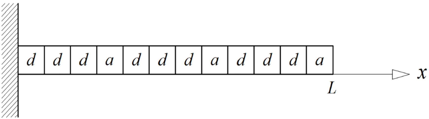
The bar is discretised into 100 nodes with interaction distance 3dx, where dx represents the distance between successive nodes. The reduced model consists of every fourth node in the detailed model, as shown in Figure 1, in which retained nodes are designated with letter ‘a’ and deleted nodes are designated with letter ‘d’.

Figure 1.

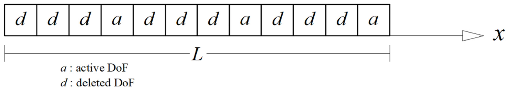
The one-dimensional reduction process.

The micromodulus of the detailed model and that of the reduced model are shown in Figure 2. The micromodulus function of the reduced model, as can be seen from Figure 2, is defined only at the retained DoFs.

Figure 2.

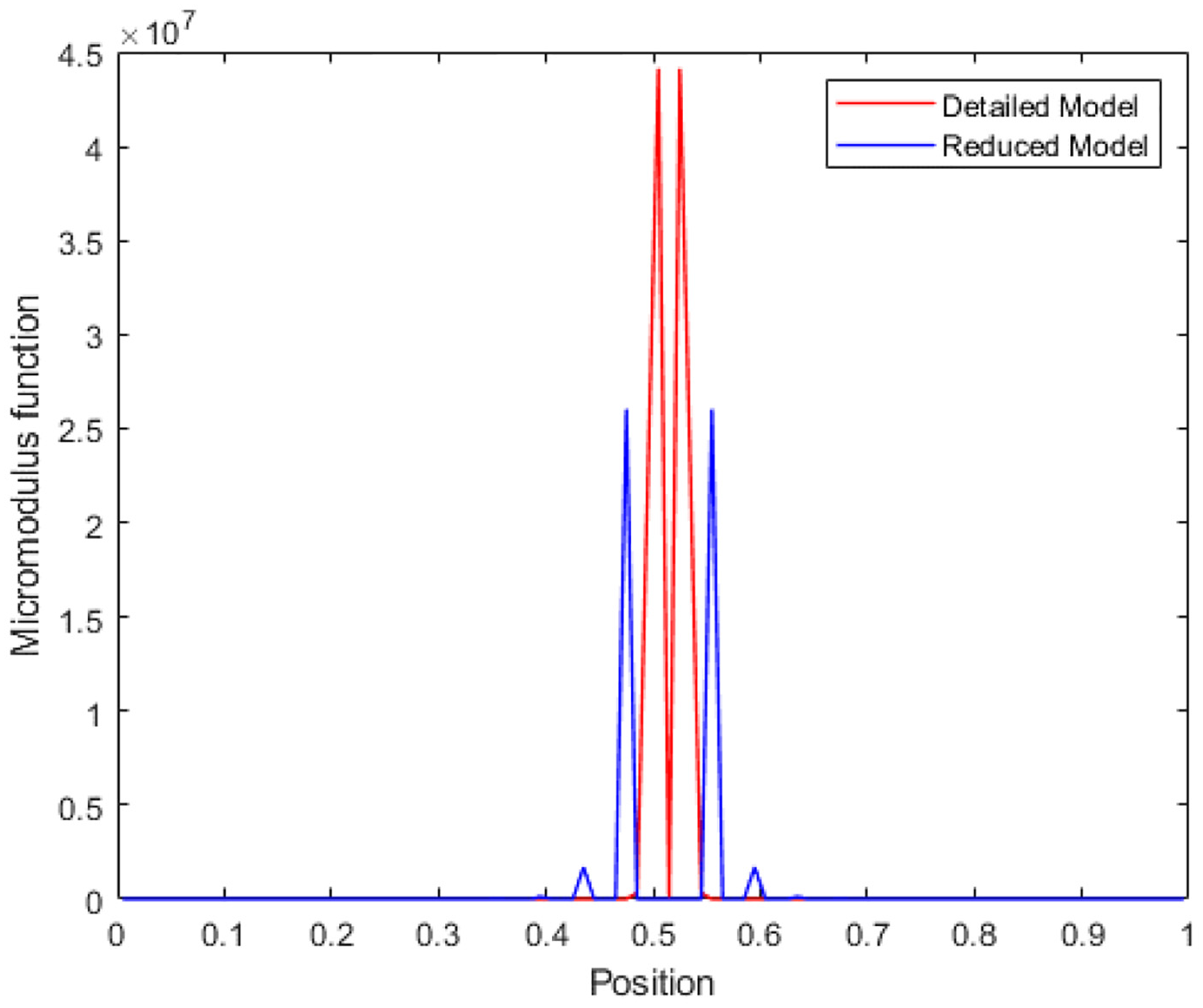
Coarsening of one-dimensional micromodulus function.

5. Numerical results

5.1. Reduction of static problems

In this section, a series of numerical experiments will be outlined to illustrate the application of this model reduction technique in coarsening one- and two-dimensional peridynamic models.

5.1.1. A bar with periodic microstructure

Consider a composite bar of length 1.0 and a periodic microstructure consisting of alternate strips $S_{\mathrm{hard}}$ and $S_{\mathrm{soft}}$ of hard and soft materials, respectively, as shown in Figure 3. Each strip is 0.05 in length. The interaction distance, $\delta$ , in both hard and soft materials is 3dx. The micromodulus of the composite system is

$$\mathrm{C}\left(\xi \right)=\{\begin{array}{cc}10.0(1-\frac{\left|\xi \right|}{\delta }),\hfill & \mathrm{if}|q-x|\le \delta \mathrm{and}(x\in S_{\mathrm{hard}}\mathrm{and}q\in S_{\mathrm{hard}})\hfill \\ \multicolumn{1}{c}{1.0(1-\frac{\left|\xi \right|}{\delta }),}& \mathrm{if}|q-x|\le \delta \mathrm{and}(x\in S_{\mathrm{soft}}\mathrm{or}q\in S_{\mathrm{soft}})\hfill \\ \multicolumn{1}{c}{0,}& \mathrm{otherwise}\hfill \end{array}$$

(36)

Figure 3.

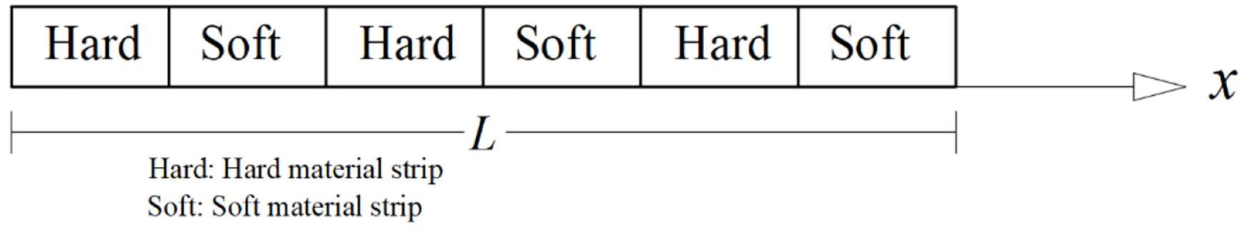
Composite bar showing hard and soft material strips.

Bonds with both ends in a hard strip are assigned hard material properties, otherwise they are given soft material properties. The coarsening of the detailed model is schematically represented in Figure 1. Every fourth material point in the detailed model is retained as an active point in the coarsened model. In the detailed model, a force density of $b=0.002$ is applied to the rightmost material point, while the leftmost material point is constrained from movement. Figure 4 shows the displacement fields of the detailed and coarsened models.

Figure 4.

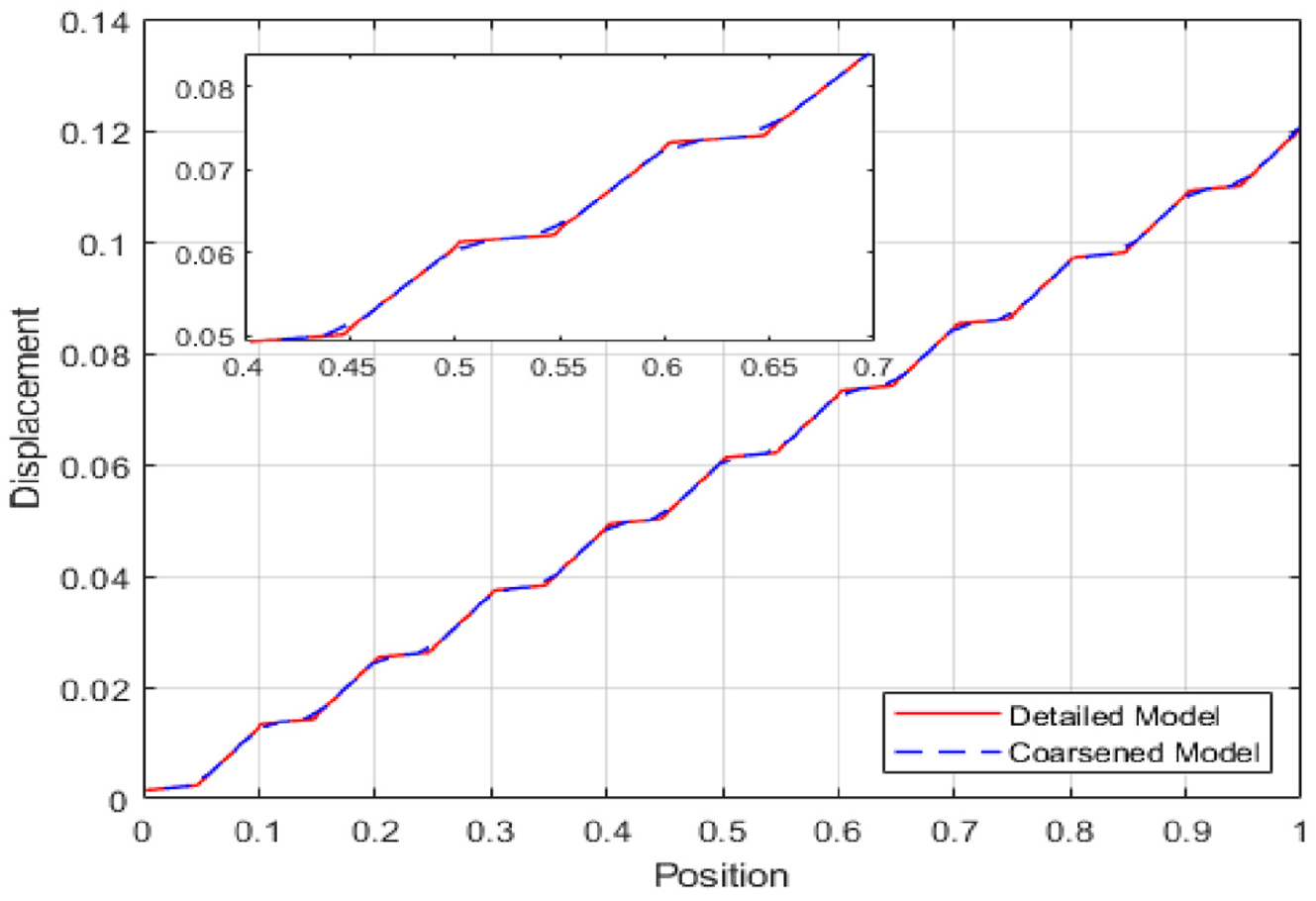
Displacement fields for detailed and coarsened models.

Results of displacement fields from simulations of both the detailed and reduced models show an exact match for all shared material points between the two models and hence both have the same global stretch. However, as expected, the reduced model reflects less resolution of microstructural information than the detailed model.

5.1.2. Reduction of peridynamic plate static model

Static condensation can be employed in the reduction of static models of peridynamic plates. The motivation for this may arise from the need to analyse a very large DoF model, if the key focus is in determining the global response of the system without the need for a very detailed model. The objective in this example is to employ static condensation to eliminate all DoFs except those corresponding to the nodes located at the vertices of the plate shown in Figure 5. The bottom length of the plate is 1.0, while all other edges of the plate are of length 0.5. The micromodulus function of the plate material has the form

$$\begin{array}{cc}\mathrm{C}\left(\xi \right)=10.0(1-\frac{\left|\xi \right|}{\delta }),\hfill & \mathrm{if}|q-x|\le \delta \hfill \end{array}.$$

(37)

Figure 5.

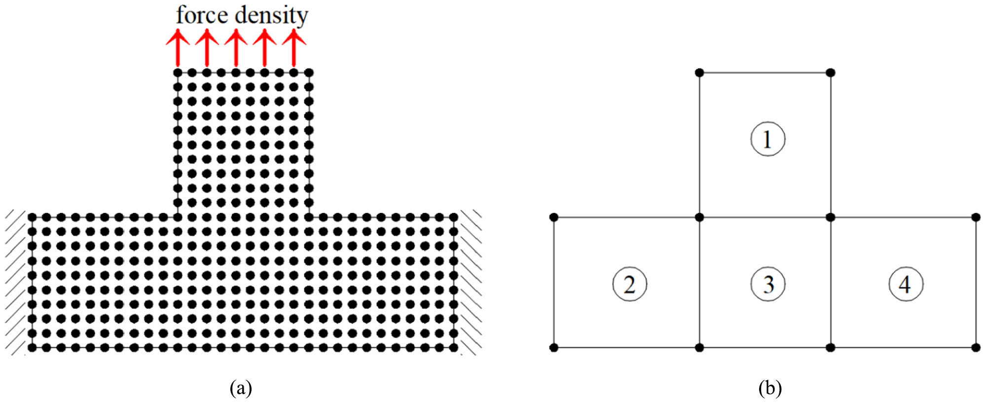
Peridynamic model of plate for static response analysis.

The maximum interaction distance $\delta =3\mathrm{dx}$ , where dx is the horizontal distance between nodes. A body force density of 0.001 is applied to the boundary nodes at the topmost edge of the plate, as shown in Figure 5(a). The detailed model is discretised into 100 material points.

The reduction procedure is achieved by condensing a group of nodes to form a substructure. At the end of the procedure, we are left with four substructures bounded by ten ‘supernodes’, as shown in Figure 5(b). As shown in Figures 6 and 7, the displacement results from the analysis of both detailed and condensed models give solutions that are exact.

Figure 6.

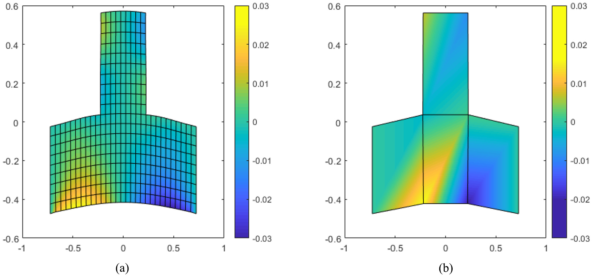
Displacement profile in x-direction: (a) detailed model; (b) coarsened model.

Figure 7.

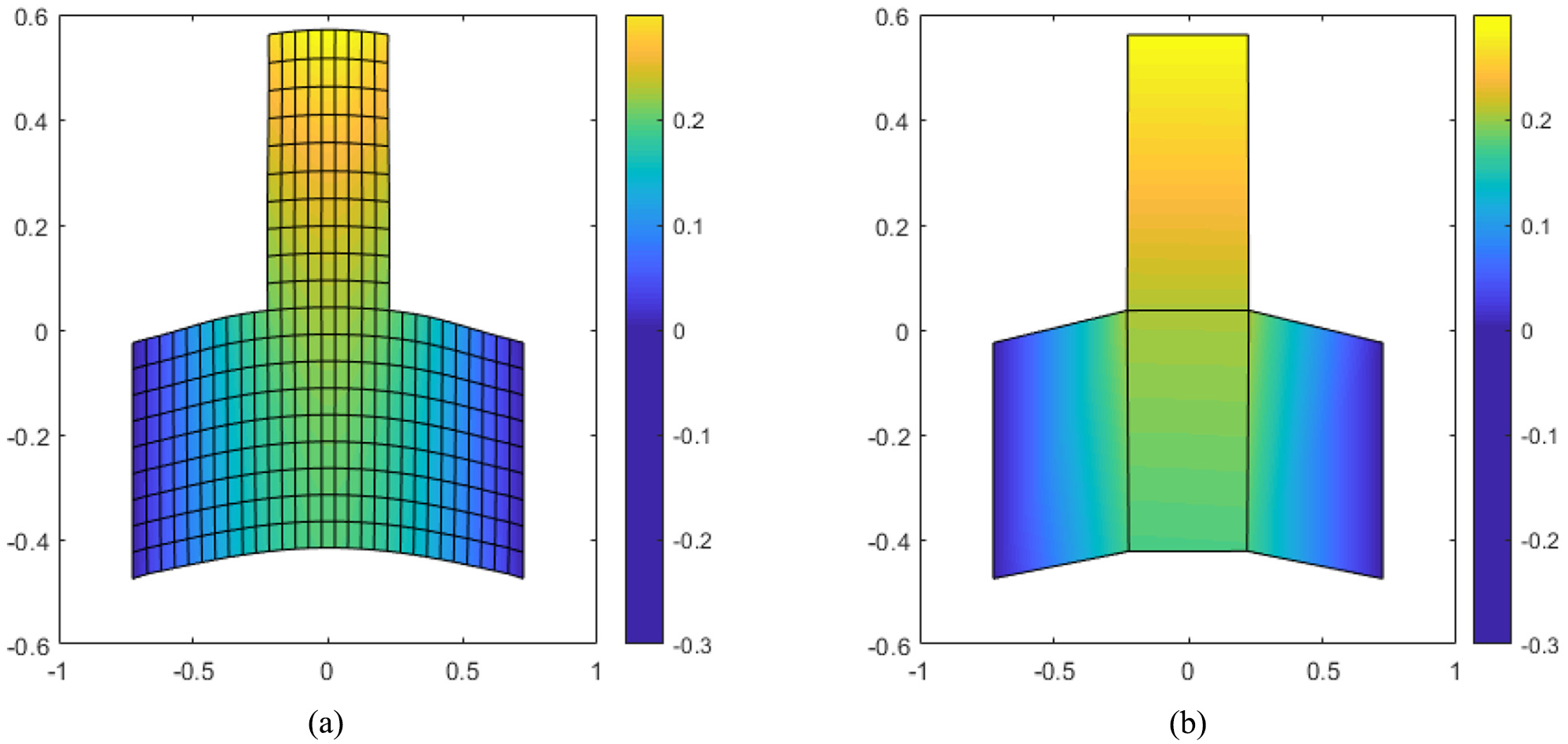
Displacement profile in y-direction: (a) detailed model; (b) coarsened model.

5.2. Reduced eigenproblems

5.2.1. A bar with one end fixed and the other free

Consider a bar of length $L=1$ and uniform cross-sectional area $A=1$ with the following material properties: Young modulus $E=1$ , density $\rho =1$ . Let the bar be fixed at one end and free at the other end, as shown in Figure 8.

Figure 8.

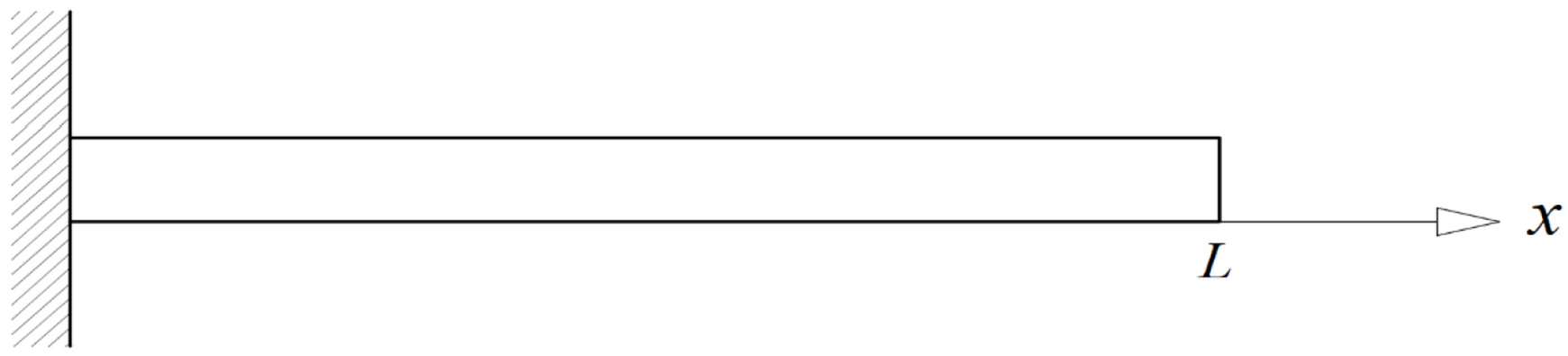
A bar with one end fixed and one end free.

To numerically compute the natural frequencies and mode shapes arising from equation (33), the given bar is discretised into 1000 nodes. The interaction distance characteristic of the bar material, $\delta$ , is assumed to be 3dx, with dx being the distance between nodes. The material is assumed to have a micromodulus function of the form

$$C\left(\xi \right)=\frac{2E}{A{\delta }^2\left|\xi \right|}.$$

(38)

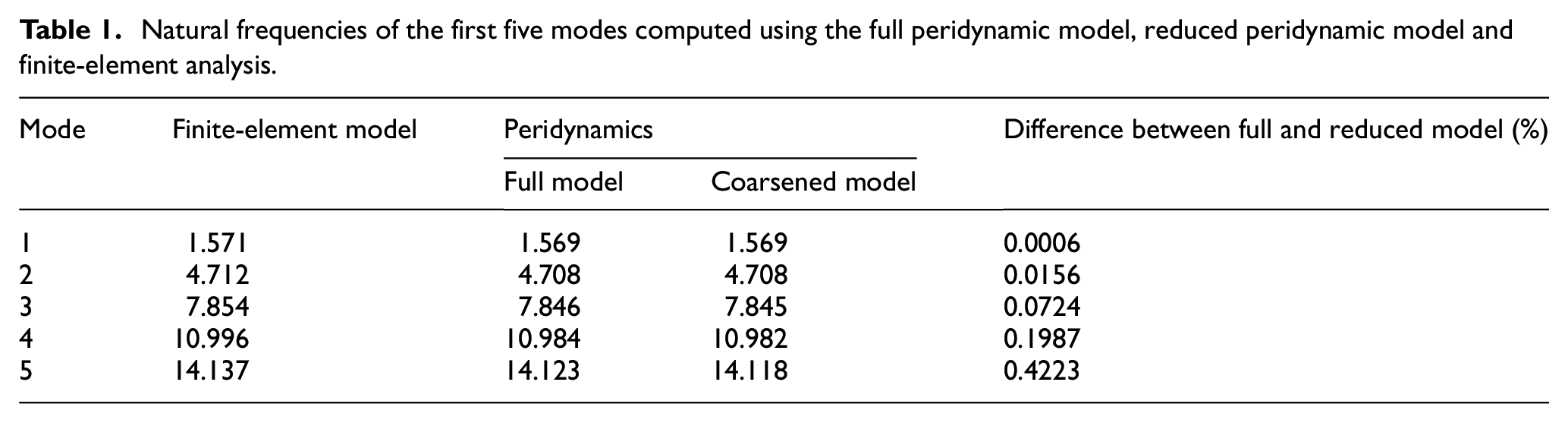
The first five lowest frequencies of the bar, as computed from equation (31), are shown in Table 1. These frequencies were then validated against frequencies obtained from the characteristic equation of the corresponding finite-element model of the bar. The eigenvalues of the first 50 modes are presented in Figure 9.

Table 1.

Natural frequencies of the first five modes computed using the full peridynamic model, reduced peridynamic model and finite-element analysis.

Mode	Finite-element model	Peridynamics		Difference between full and reduced model (%)
		Full model	Coarsened model
1	1.571	1.569	1.569	0.0006
2	4.712	4.708	4.708	0.0156
3	7.854	7.846	7.845	0.0724
4	10.996	10.984	10.982	0.1987
5	14.137	14.123	14.118	0.4223

Figure 9.

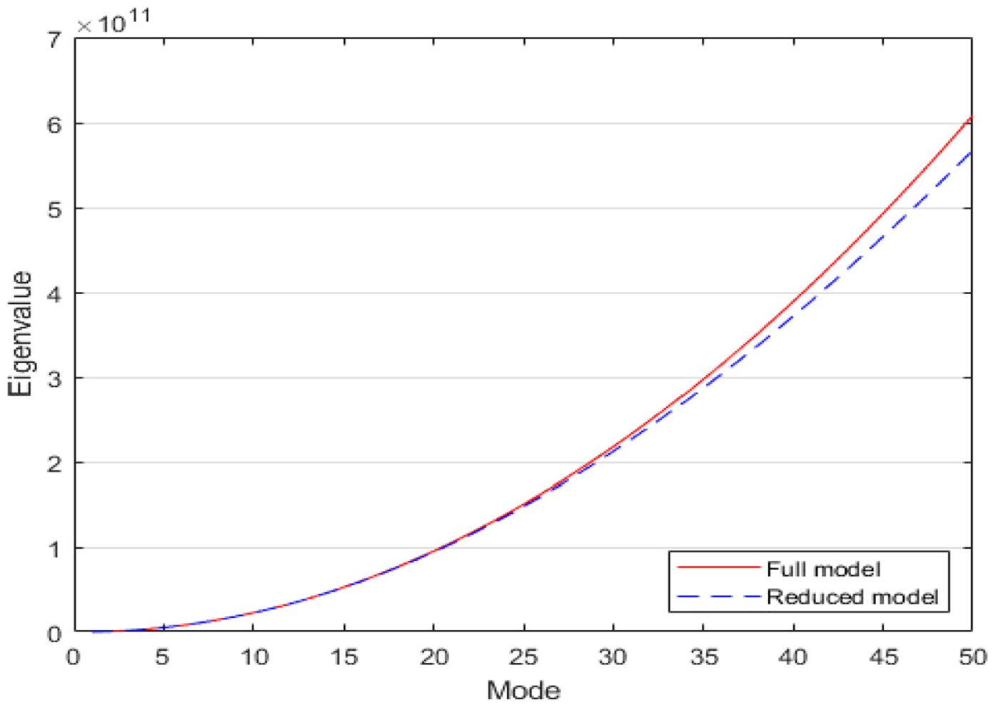
Comparison of eigenvalues from the full peridynamic model and coarsened model.

The percentage difference between the natural frequencies computed from modal analysis of the full peridynamic model and the reduced-order peridynamic model, as presented in Table 1, shows a difference that ranges from 0.0006% to 0.4223%. This error margin, coupled with the results presented in Figure 9, shows that the reduced model can accurately reproduce the lower eigenproperties of the full model.

5.3. Reduction of dynamic problems

In this section, the static condensation technique will be applied to reduce the order of a peridynamic model and determine its time-history response. The objective is to determine the effectiveness of the model reduction technique in predicting the dynamic response of a given model despite the use of fewer DoFs. To illustrate the capabilities and limitation of the dynamic condensation technique, the bar shown in Figure 8 will be subjected to various excitations to determine the accuracy of the dynamic response predicted from the reduced-order model. The bar will be assumed to have a Young modulus of $200\mathrm{GPa}$ and a density of $7850\mathrm{Kg}/{\mathrm{m}}^3$ . The numerical integration method used to integrate the discretised peridynamic equation of motion for the transient analysis is the forward Euler method.

5.3.1. Free vibration of a peridynamic bar

The transient response of the peridynamic bar will be studied. Three initial condition cases will be considered.

5.3.1.1. Case 1: displacement-induced initial excitation

In this scenario, the bar is given an initial constant strain of 0.0001. The excitation is immediately removed to allow for free vibration of the bar. A transient analysis of the full peridynamic model of the bar was conducted. The condensation process proceeded by retaining every forth node of the full peridynamic model, as shown in Figure 10.

Figure 10.

Discretisation and condensation of the full peridynamic model.

The results of the time-history response of material points located at $x=0.0995$ and $x=0.4995$ arising from both the full peridynamic model and the reduced model, respectively, are shown in Figure 11(a and b). Figure 12 shows the displacement values of all nodes at the 5000th, 10,000th, 20,000th and 26,000th time steps. These results show that the reduced model closely reproduces the dynamic response of the original peridynamic model. However, as can be seen from Figure 11, there are some errors, arising from the neglect of inertia effects at the deleted DoF.

Figure 11.

Time-history response of material points located at (a) x = 0.0995 and (b) x = 0.4995, for both full and coarsened models.

Figure 12.

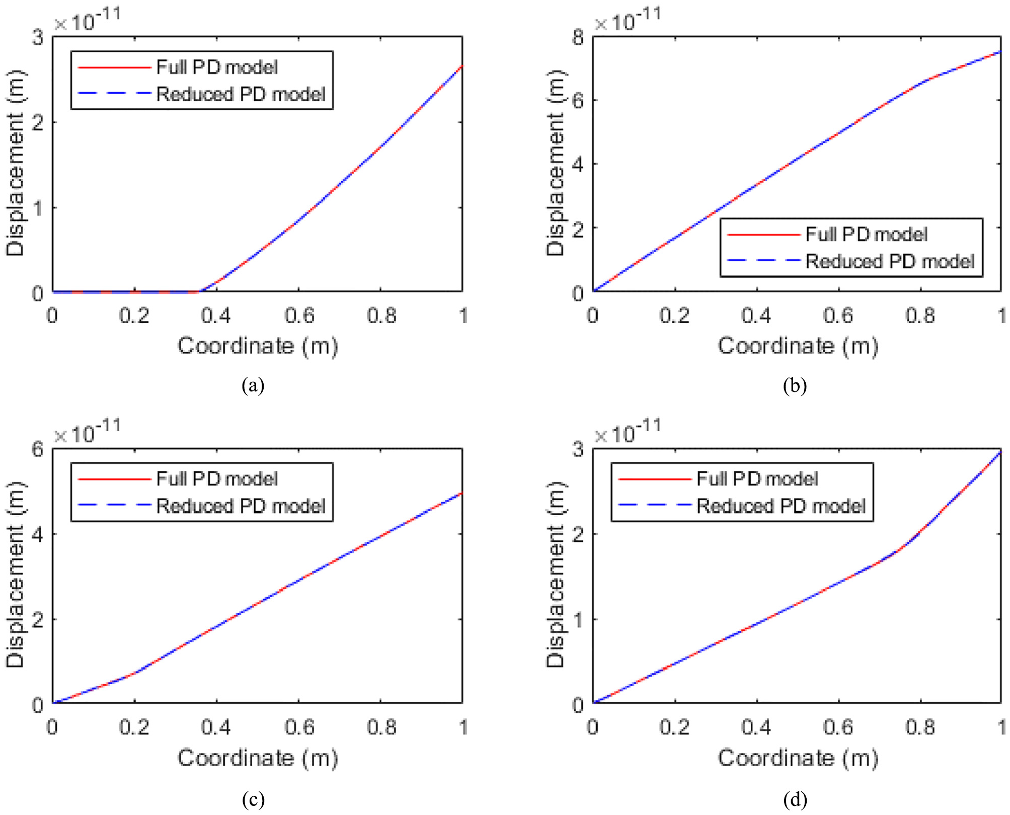
Displacement values at all nodes at (a) 5000th time step, (b) 10,000th time step, (c) 20,000th time step and (d) 26,000th time step.

5.3.1.2. Case 2: force-induced initial excitation

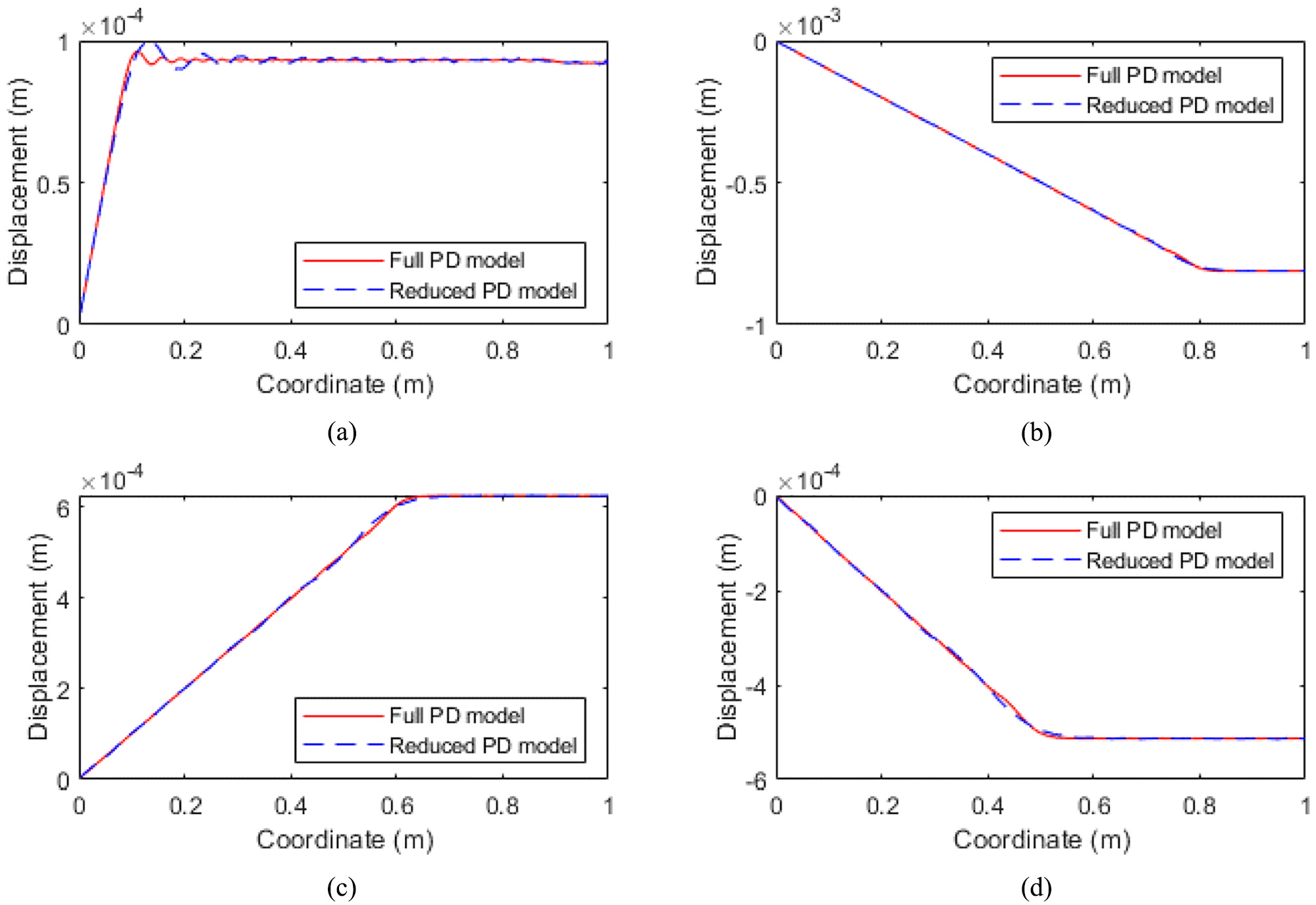
In this case study, an initial constant body force density of $1\times {10}^4\mathrm{kN}/{\mathrm{m}}^3$ is applied to every second node of the discretised peridynamic bar and the force is immediately removed to allow for a free vibration of the bar. Equation (24) is used to condense the mass matrix, the stiffness matrix and the force vector. The time-history responses of points located at $x=0.0995,x=0.2995,x=0.4995$ and $x=0.7995$ for both the full and reduced models are shown in Figure 13, while Figure 14 shows the displacement values for all nodes at time steps 5000, 10,000, 20,000 and 26,000. The results of the time-history analysis of the both the full peridynamic model and the reduced model show that the condensation technique can accurately reproduce the dynamic response of the full peridynamic model of the bar.

Figure 13.

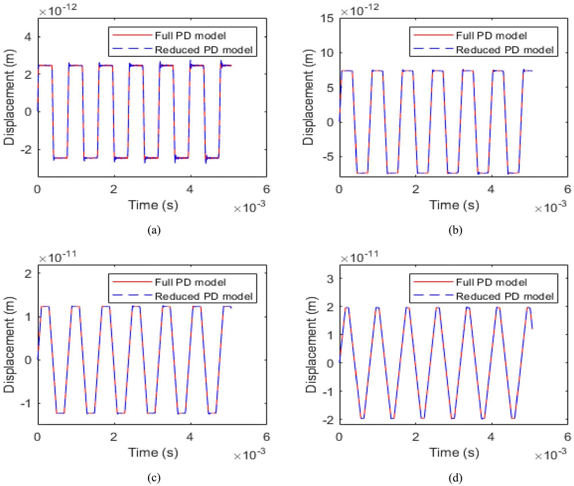
Time-history response of material points located at (a) x = 0.0995 (b) x = 0.2995 (c) x = 0.4995 and (d) x = 0.7995 for both the full peridynamic model and the coarsened model.

Figure 14.

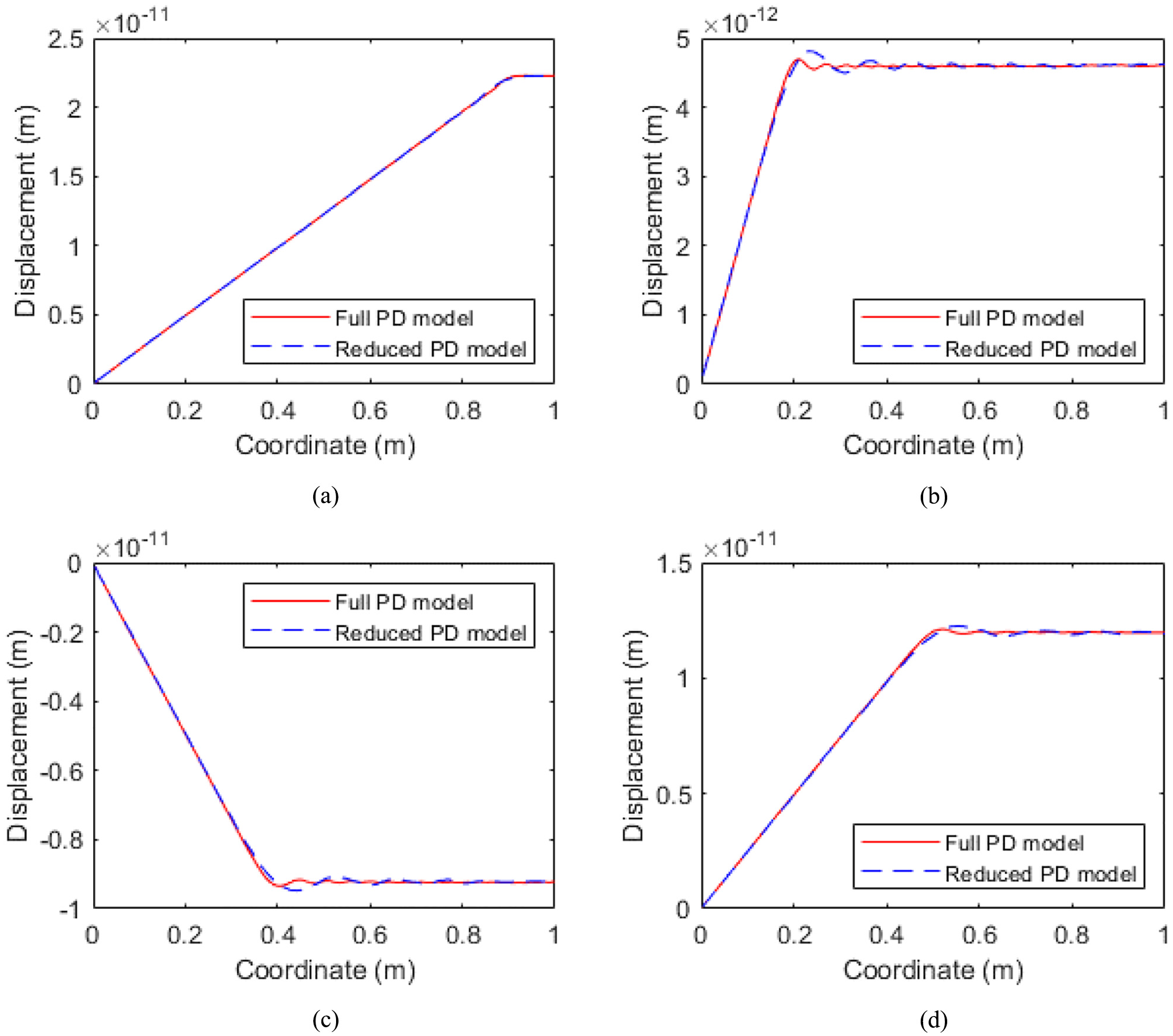
Displacement values at all nodes at (a) 5000th time step, (b) 10,000th time step, (c) 20,000th time step and (d) 26,000th time step.

5.3.2. forced vibration

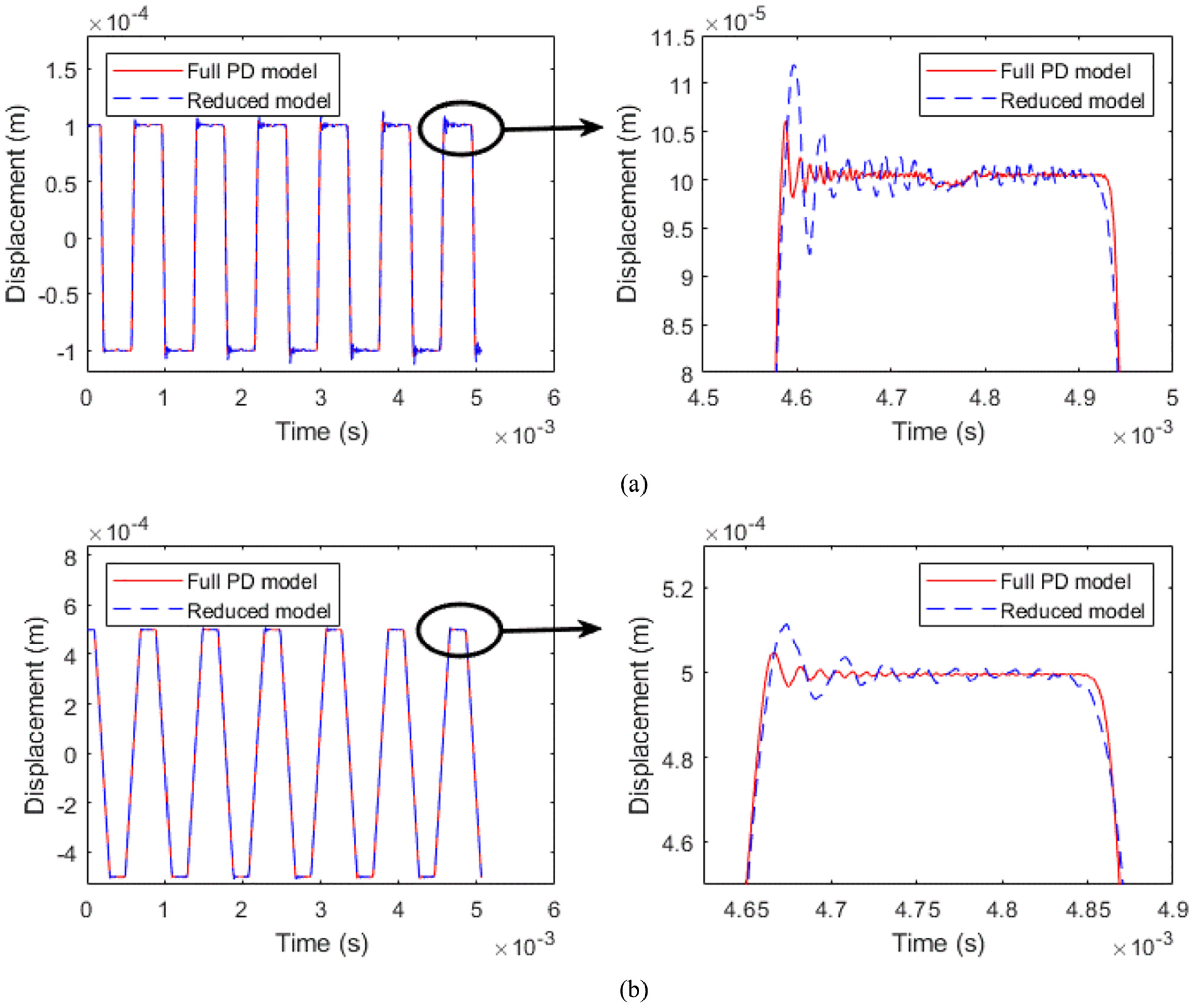
The bar in this case is assumed to be subjected to a time-dependent body force density of the form $\left\{b\left(t\right)\right\}=\left\{b_0\right\}\sin (\omega t)$ , where $b_0$ is the amplitude of excitation and $\omega$ is the frequency of excitation. The force is applied at the rightmost node of the bar.

Results from a transient analysis of the full and coarsened models for $b_0=1\times {10}^4\mathrm{kN}/{\mathrm{m}}^3$ and $\omega =5\mathrm{rad}/\mathrm{s}$ for a total of 86,000 time steps are shown in Figures 15 and 16. The dynamic response of the full peridynamic model was accurately predicted using the coarsened model.

Figure 15.

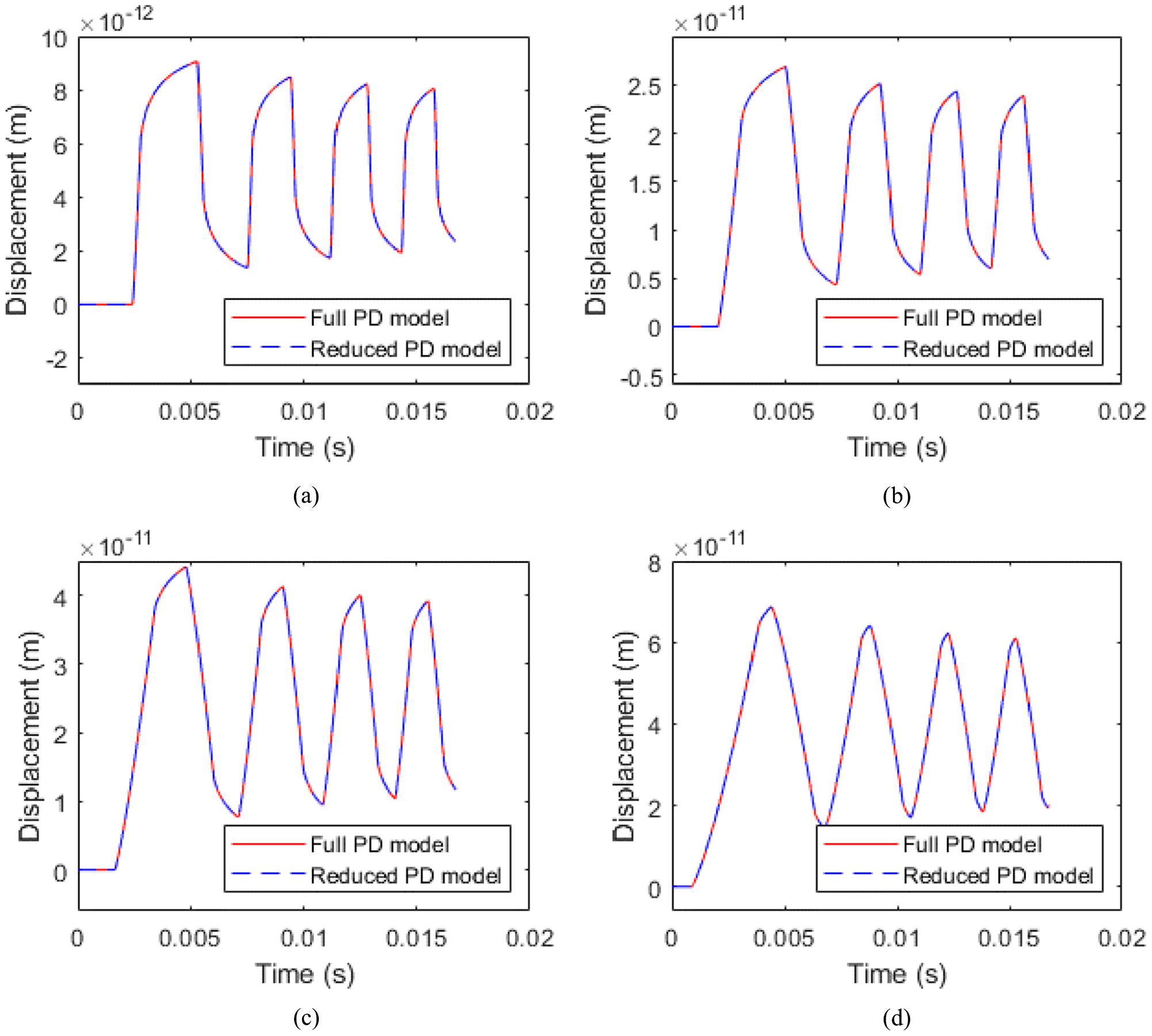
Time-history response of material points located at x = 0.0995, 0.2995, 0.4995 and 0.7995 for both the full peridynamic model and coarsened model.

Figure 16.

Displacement values at all nodes at (a) 10,000th time step, (b) 20,000th time step, (c) 50,000th time step, and (d) 86,000th time step.

6. Conclusion

A model reduction procedure for peridynamic systems based on static condensation has been developed and investigated in this study. The presented results of numerical experiments show that the reduction algorithm based on the static condensation technique can closely preserve the characteristics and response of the original model. In the static regime, the algorithm has proved to yield identical results to those obtained from the original model. The results of the eigenresponse prediction of the reduced model shows some errors, as shown in the eigenresponse and transient analysis; however, the results show that the proposed algorithm has capabilities of accurate prediction of dynamic response at low frequencies.