
Abstract
Over the last two decades, there have been tremendous advances in the computation of diffusion and today many key properties of materials can be accurately predicted by modelling and simulations. In this paper, we present, for the first time, comprehensive studies of interdiffusion in three dimensions, a model, simulations and experiment. The model follows from the local mass conservation with Vegard’s rule and is combined with Darken’s bi-velocity method. The approach is expressed using the nonlinear parabolic–elliptic system of strongly coupled differential equations with initial and nonlinear coupled boundary conditions. Implicit finite difference methods, preserving Vegard’s rule, are generated by some linearization and splitting ideas, in one- and two-dimensional cases. The theorems on the existence and uniqueness of solutions of the implicit difference schemes and the consistency of the difference methods are studied. The numerical results are compared with experimental data for a ternary Fe-Co-Ni system. A good agreement of both sets is revealed, which confirms the strength of the method.
Keywords
1. Introduction
Diffusion controls many chemical and physical processes; therefore, a knowledge of diffusion and the ability to study it theoretically and experimentally are very valuable in materials science. Common examples of diffusion-controlled processes are: sintering of powders, grain growth, nitriding and carburizing by vapour deposition, oxidation and diffusional creep, as well as processes applied in microelectronics devices, such as the addition of n or p impurities to semiconducting silicon, germanium or other crystals, welding, crystallization and many other alloying and metallurgical processes. Among the given examples of engineering applications, there are situations in which the solids under study do not present one-dimensional geometry. These are mainly examples of metallic joints in welding and soldiering, and of the stability of coating–substrate systems. Therefore, a knowledge of the mass transport in bodies with an arbitrary two- or three-dimensional geometry is important.
A suitable formalism for an

where

Mass conservation needs to be combined with a constitutive equation for the flux. A theory that is considered the most fundamental to describe interdiffusion in multicomponent systems is provided by linear phenomenological laws [1] combined with Onsager reciprocal relations [2, 3]. Linear phenomenological laws predict that when the system is close to the state of equilibrium and local equilibrium holds, the flows

In this equation,

and

where the superscripts “

where

which is implied by equations (1), (4) and (6). In the one-dimensional case, if the fluxes on the boundaries of a domain equal zero, then the explicit formula on

However, in the multidimensional cases, this is obviously not true. Nonetheless, the three-dimensional case has been studied, for example in [16, 17] with the use of equation (8). Taking into account equation (7), this is not a mathematical method and, physically, a part of information from the fluxes is neglected. We omit this assumption by a postulate that the drift field is a potential, i.e.
Much research has been conducted to understand the interdiffusion behaviour and its after-effects in multicomponent systems. For an extensive study, see, for example, the book by Gusak [19]. If a process is described by the diffusive model, the diffusion equation must be solved and initial and boundary conditions should be established. For two- and three-dimensional diffusion, a geometry of the solids must be assumed. Owing to many difficulties, numerical solution of the diffusion equation in three dimensions remains a challenging mathematical problem.
There have been only a few attempts to study multicomponent diffusion in the systems of an arbitrary geometry. Verbrugge et al. [20] simulated Fickian diffusion (
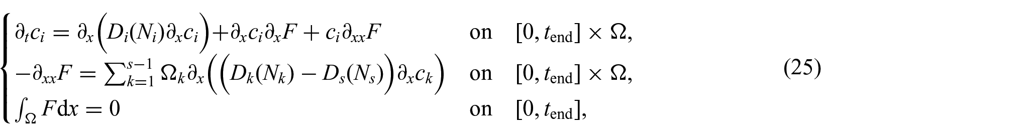
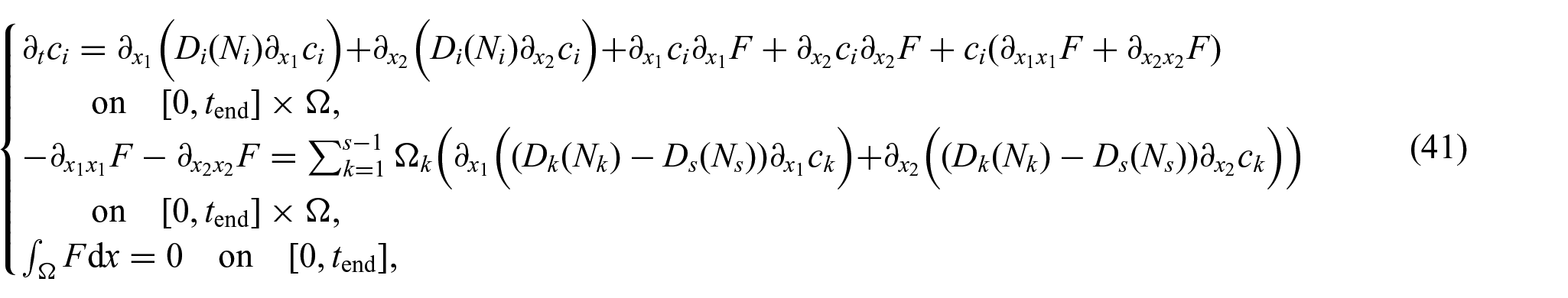
To make progress, we combine, in the present studies, computations and experiments of the interdiffusion in two-dimensional geometry. As an example, a ternary Fe-Co-Ni system is considered. A model based on Darken’s method with the use of Vegard’s rule is formulated. It is expressed by the strongly coupled nonlinear parabolic–elliptic system
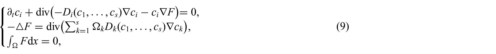
for
Let us stress that such strongly coupled systems as in our model (i.e., by the second derivatives) have seldom been investigated mathematically. Equation (9) is a little similar in the structure to the Nernst–Planck–Poisson system [36–39]. We suppose, after analysis of the papers mentioned, concerning the Nernst–Planck–Poisson model, that if the initial concentrations and the fluxes on the boundaries are sufficiently regular, then equation (9) has a unique regular solution. It is a completely new model and our analytical investigations are not finished.
The paper is organized in the following way. In Section 2, the initial–boundary differential problem is formulated. Section 3 deals with the construction of the implicit finite difference methods, the analysis of the existence and the uniqueness of solutions to the suitable difference schemes and consistency of the difference methods in the one- and two-dimensional cases, respectively. Experimental and simulated data are discussed in Section 4. We show preparation of the diffusion couple, diffusion experiment, concentration maps and chosen profiles. The diffusion fluxes and drift velocity are computed and the time evolution is simulated. In Section 5, the results are summarized.
2. Interdiffusion model
In [23, 24], the following model of interdiffusion is constructed. Let an open and bounded set

The following data are given:
(a)
(b)
(c)
(d)
The following functions are unknown:
(a)
(b)
We assume that each component of the mixture is a continuous medium, i.e. it satisfies the local mass conservation law (continuity equation)

where

is a flux of the

The solutions of the interdiffusion in the
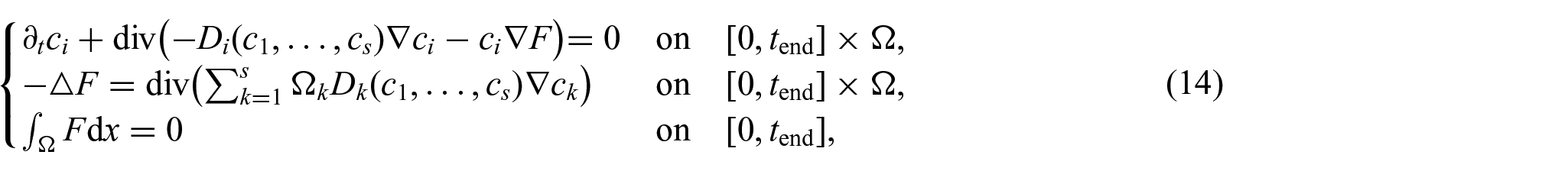
with the initial conditions

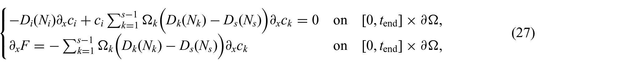
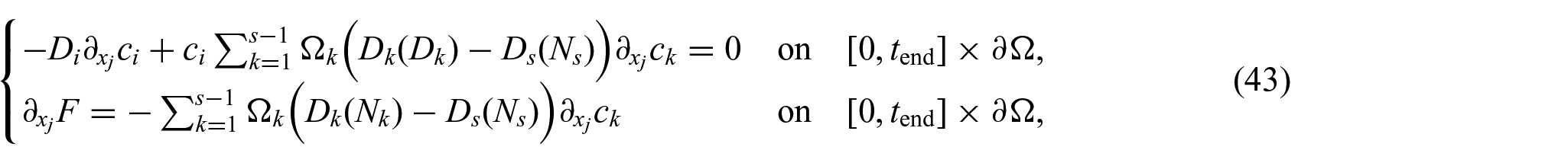
and the coupled nonlinear boundary conditions
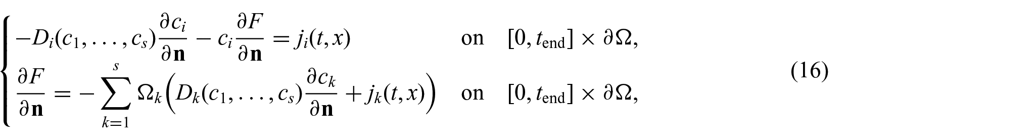
where
We assume the constant overall volume; thus, from incompressible transport

This can be treated as the compatibility condition to the elliptic subsystem to be well posed. This condition also follows immediately from the Gauss theorem.
Moreover, we assume the Vegard rule on the initial concentrations


on

on


leads to a differential algebraic system like equations (11) and (13), with
3. Implicit difference method
3.1. Case n = 1
Let
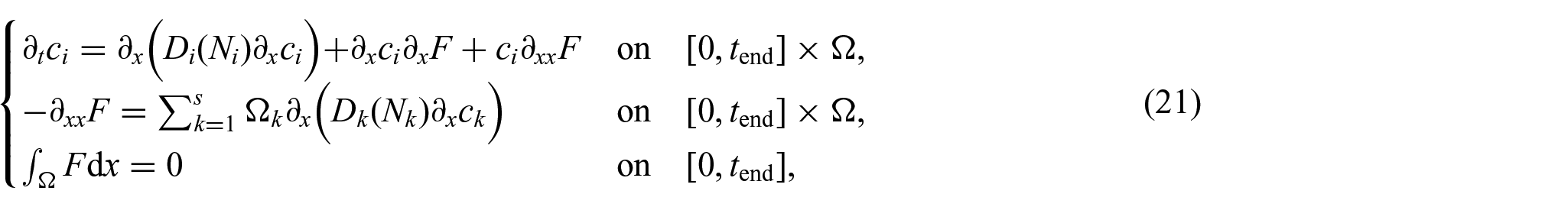


and then equations (21) to (23) are reduced as follows:


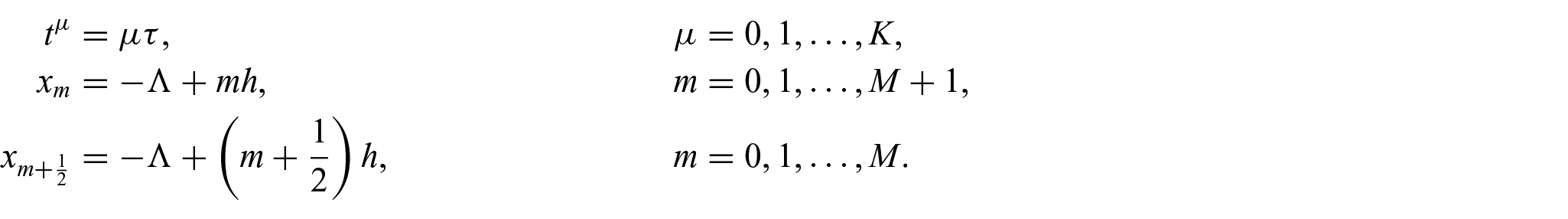
Define a mesh on
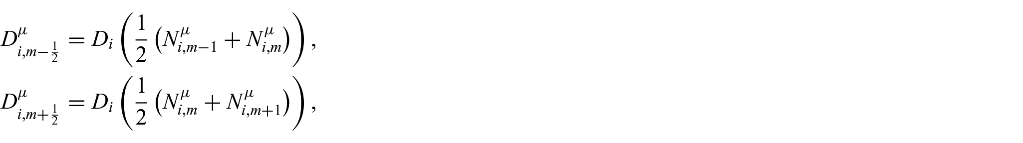
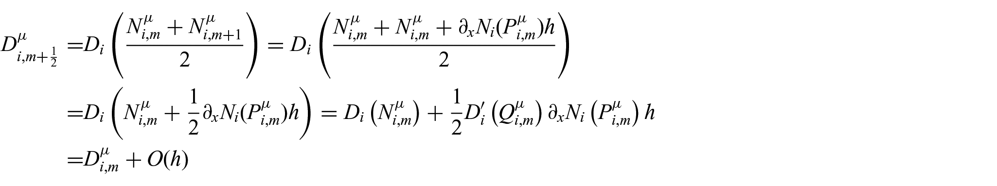
The terms

where
for

for
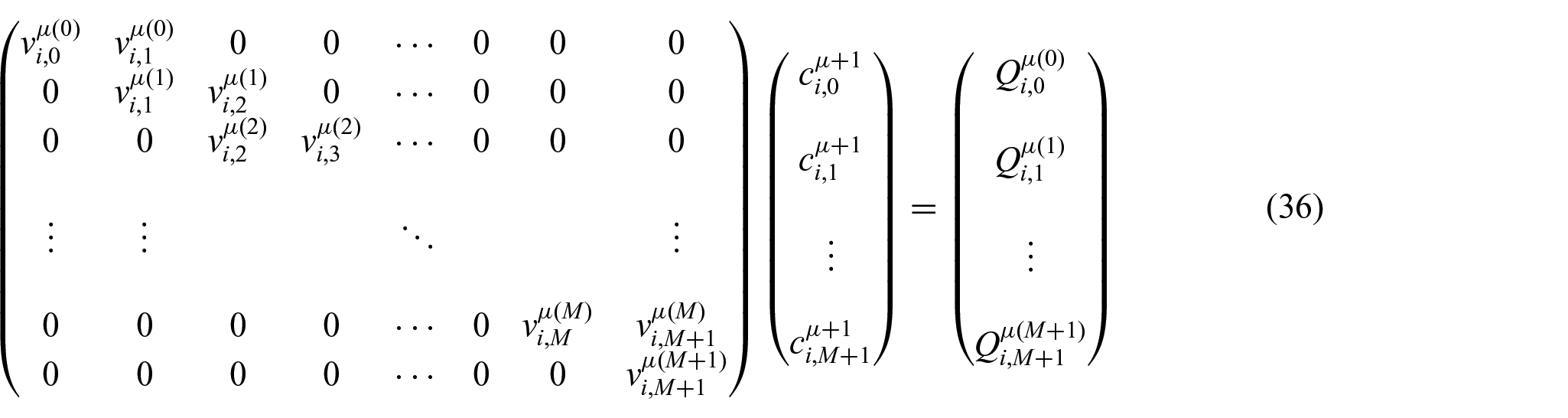
We define an implicit difference scheme for the elliptic subsystem on the potential
for
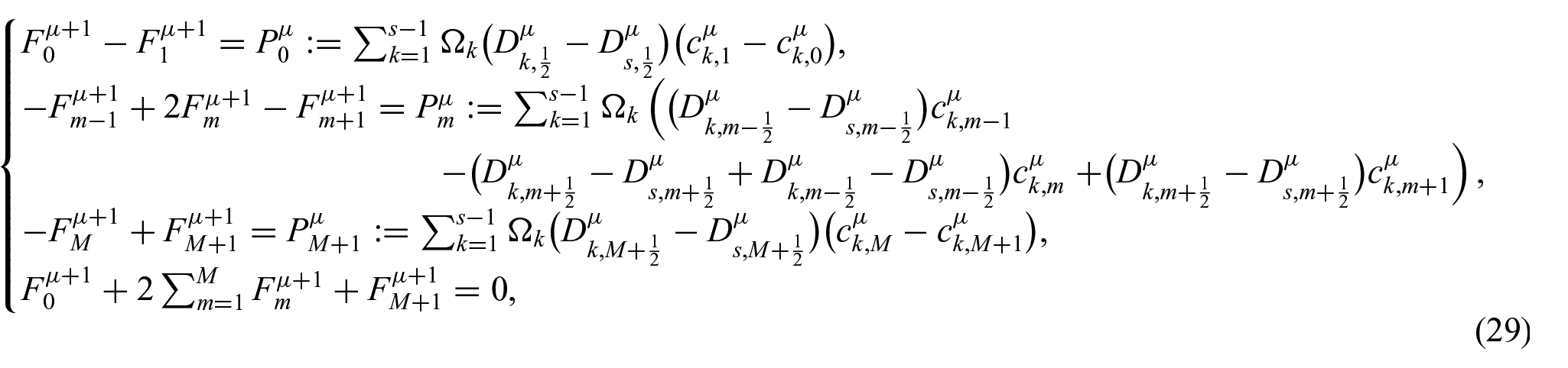
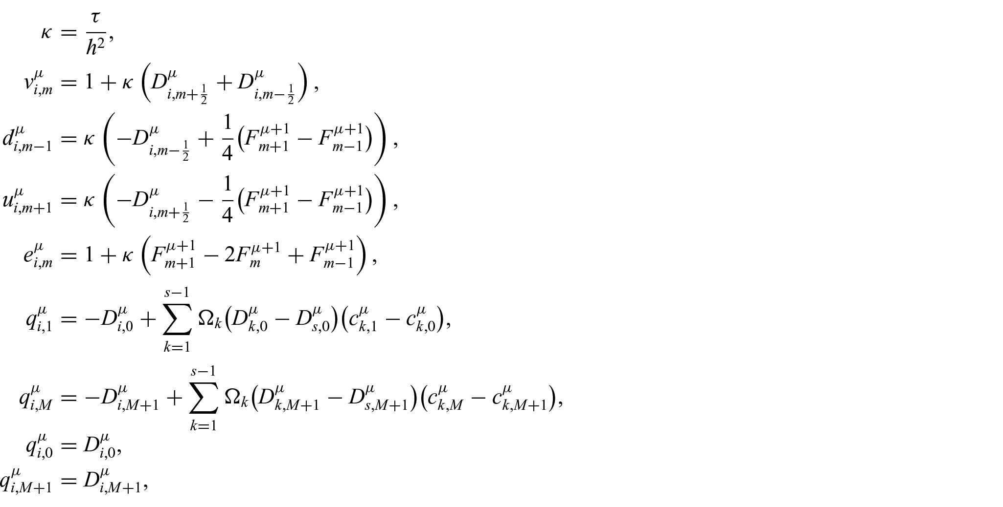
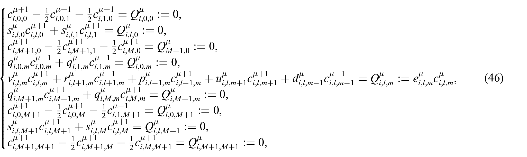
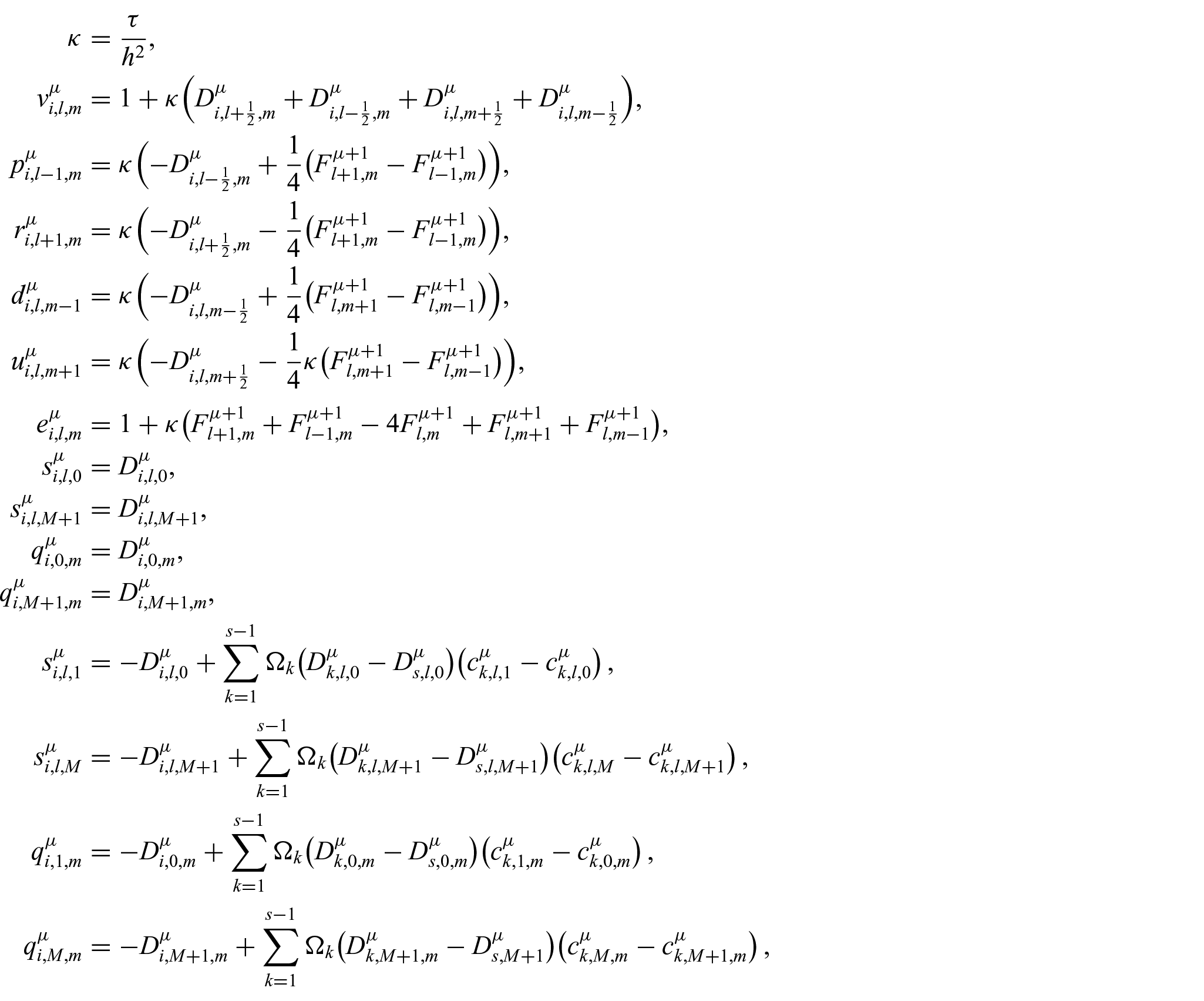
Then we define an implicit difference scheme for the parabolic subsystem on the concentrations
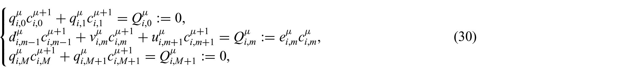
where
for
If the steps
with
(1) For all the steps

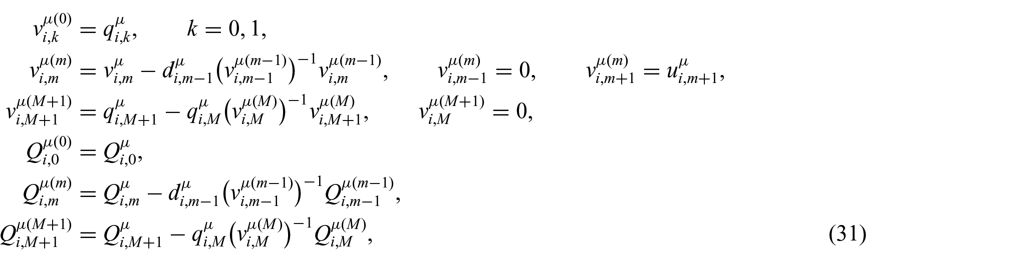
(ii) Equation (30) has exactly one solution
for
It follows from elementary calculations that
with the square
Now we will prove point (ii). Let any
Hence, equation (30) has a unique solution
Analogously, in the boundary points:
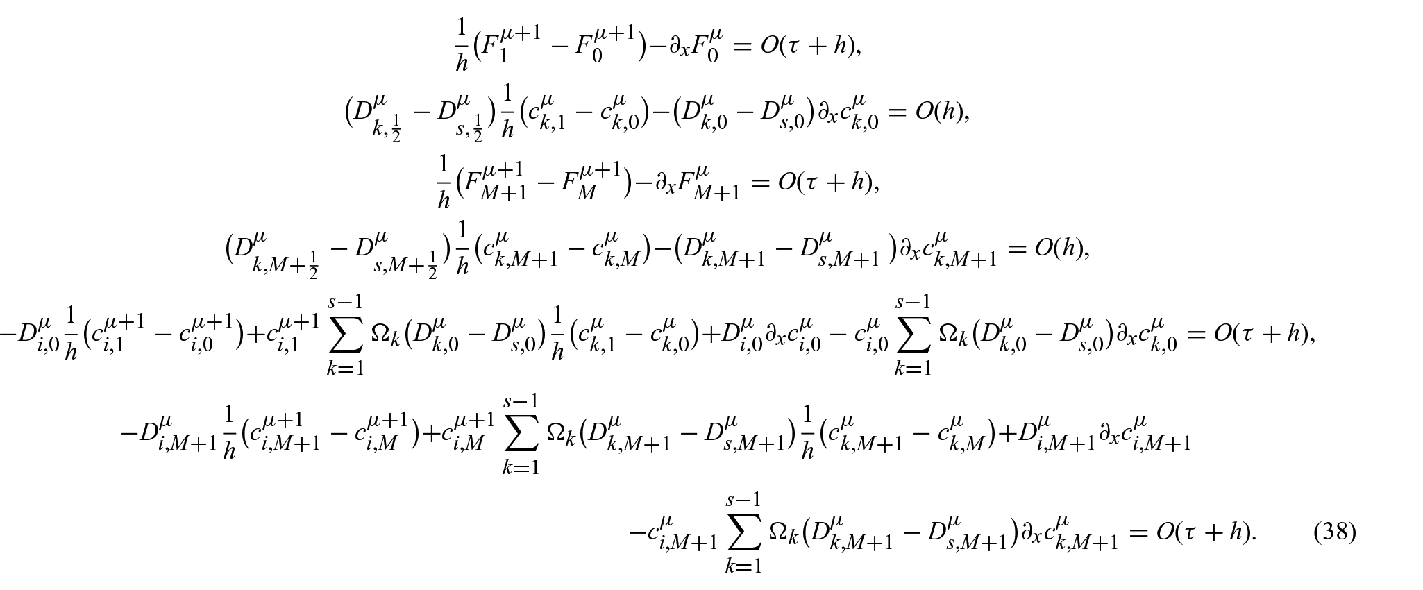
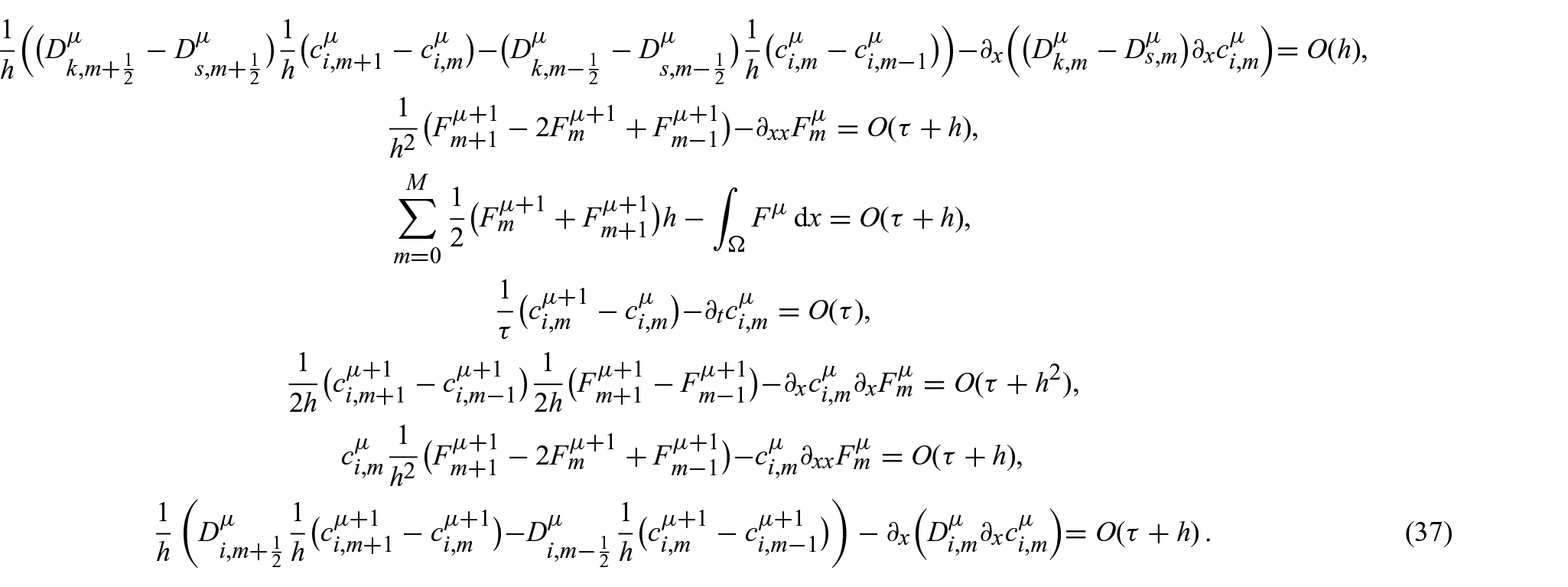
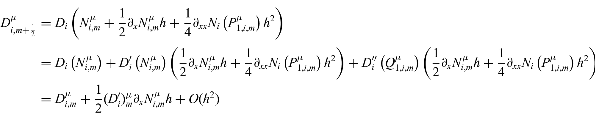
We will justify the most difficult last formula in equation (37) only. We will use the Taylor formula for the concentrations

where

Moreover,
for some intermediate points

In consequence,

Making similar calculations as before, we obtain
for some intermediate points

Hence,

Equations (39) and (40) imply
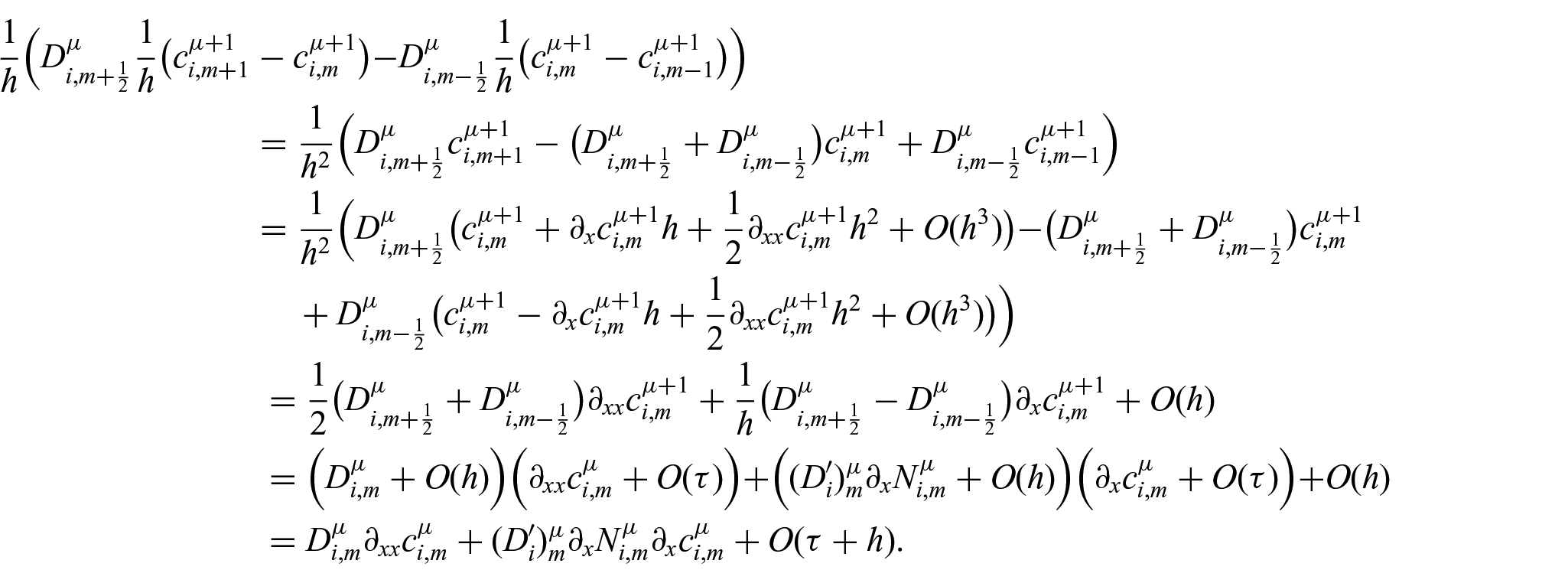
It follows immediately from the form of equations (25) to (27), (29), (30), (37) and (38) that our difference method is consistent and the truncation errors
3.2. Case n = 2
Let

with

We assume, additionally, that

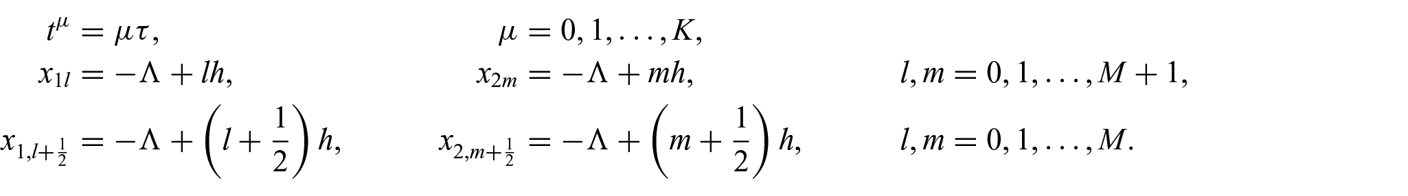
We define a mesh on
The terms
where
for

for
We define an implicit difference scheme for the elliptic subsystem on the potential
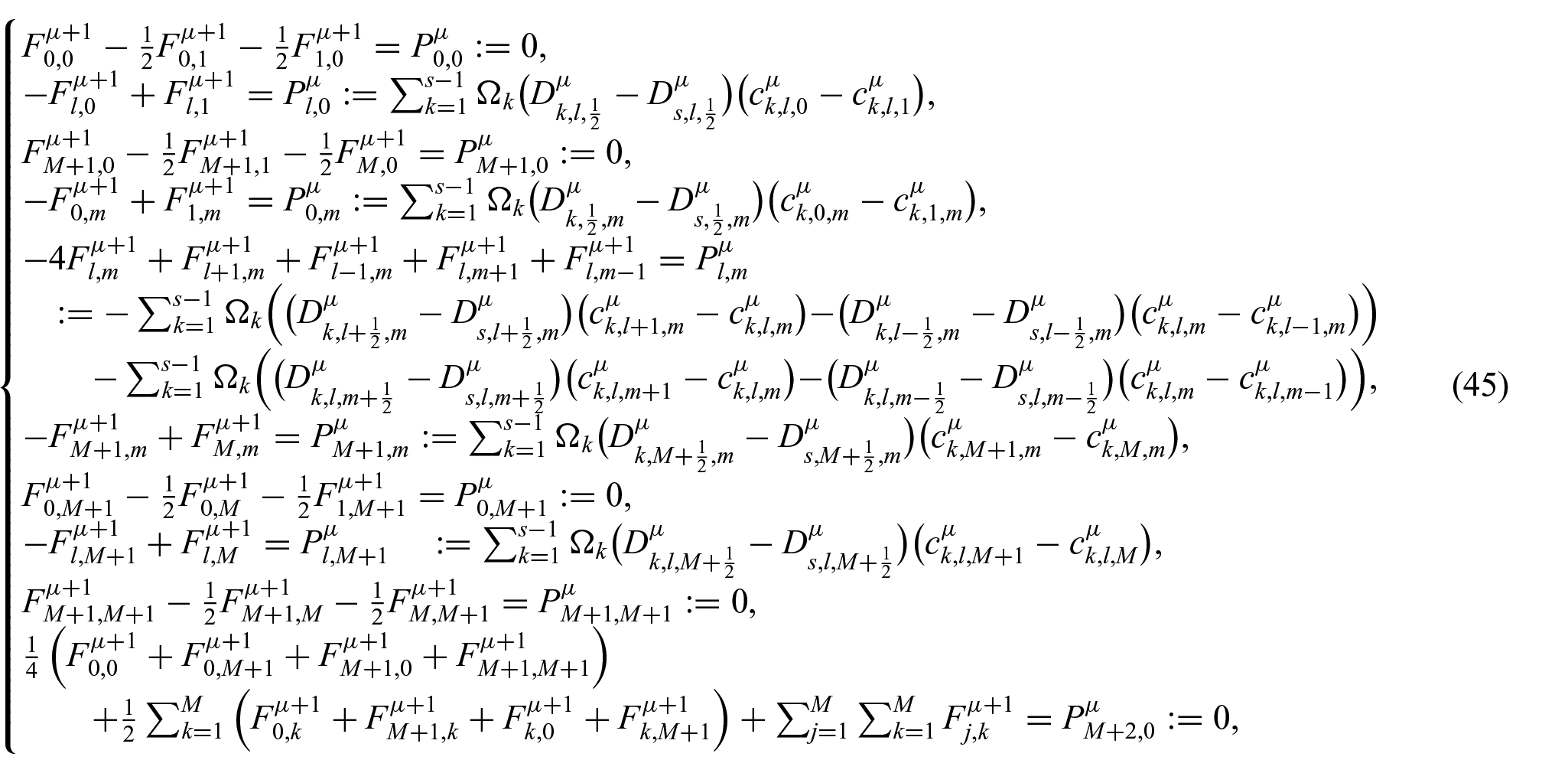
for
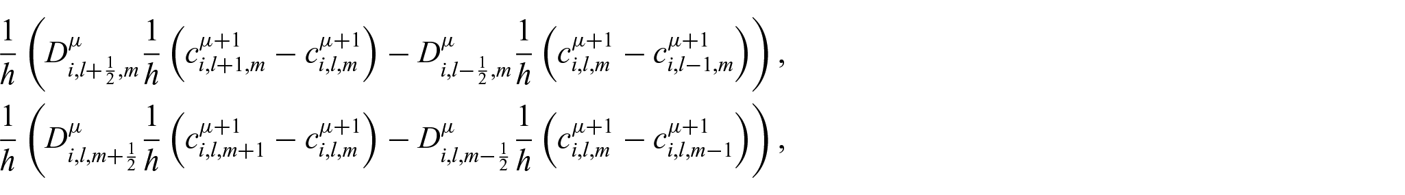
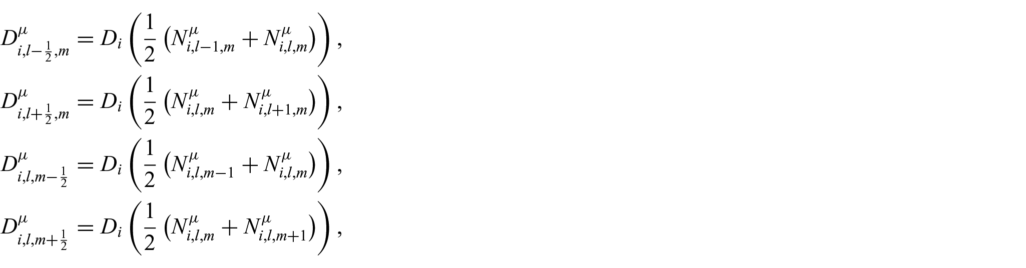
Then we define an implicit difference scheme for the parabolic subsystem on the concentrations
where
for
4. Experiment and simulations
In this section, we explicitly show the results, experiment and simulations. We start with the diffusion multiple experiment and perform the computations of the concentration maps and profiles and the drift velocity.
4.1. Diffusion multiple
To validate the model and numerical simulations, a diffusion multiple was prepared from pure Fe, Co and Ni, each with a purity of at least 99.95%, provided by Alfa Aesar. In subsequent stages, the materials were polished down to
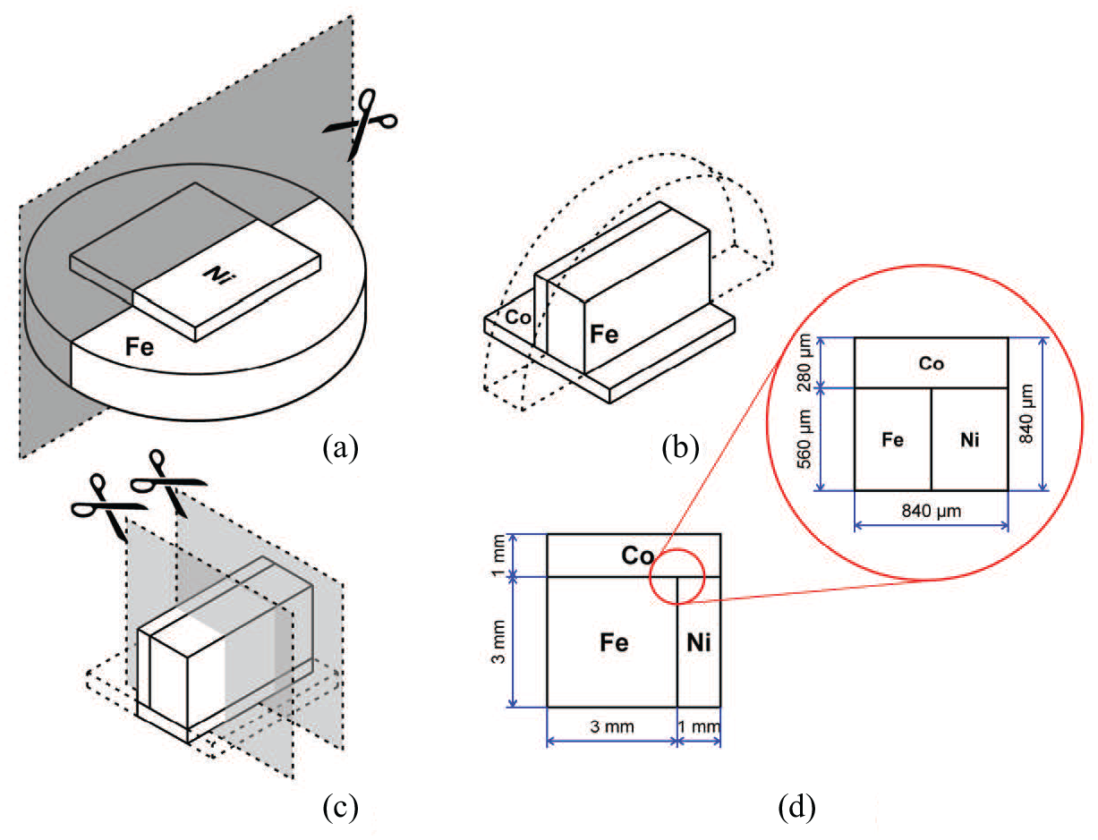
Steps to prepare the Fe-Co-Ni multiple sample: (a) Fe|Ni couple, (b) multiple, (c) cutting, (d) sample; the inset shows an examined area.
The Fe, Co and Ni concentration maps were measured with a resolution of
4.2. Calculations
We consider a ternary Fe-Co-Ni mixture and assume the following data:
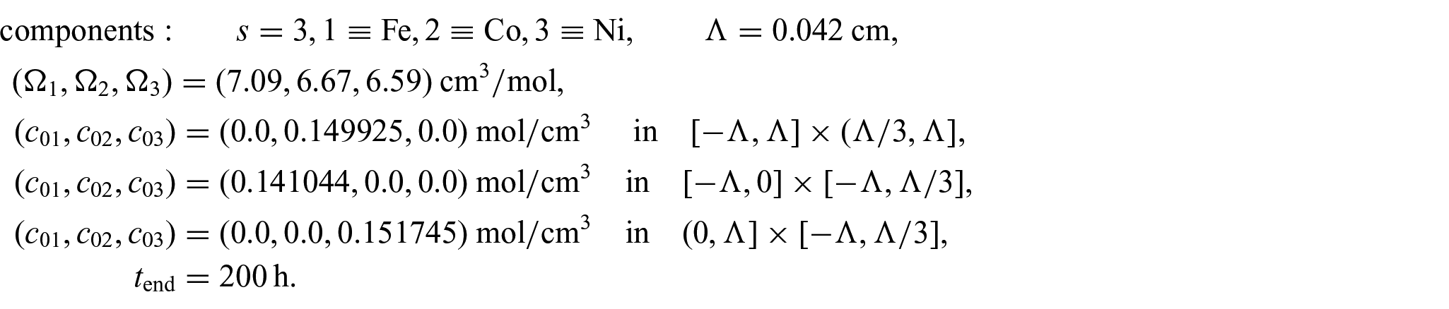
For the mixture, the diffusion coefficients
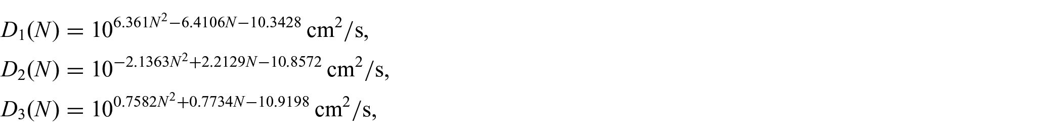
where
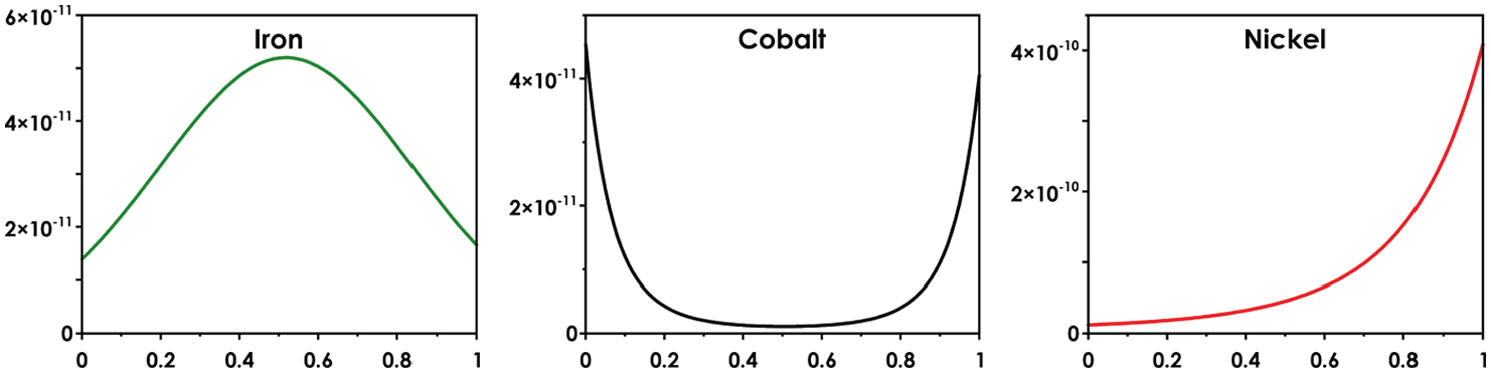
Diffusion coefficients, cm2/s, for the components in the ternary Fe-Co-Ni mixture.
The one-dimensional concentration profiles were calculated using the difference method presented in case
4.2.1. Maps and profiles: comparison with experiment
Experimental concentration maps, processed with the Savitzky–Golay filter to reduce noise, are shown in Figure 3(a). The scanning electron micrographs reveal the Frenkel porosity in iron. For binary couples chosen from the multiple, the positions of the Matano’s planes were calculated using the procedure of Leszczyński et al. [45]. They were used to simulate the interdiffusion in the multiple. The resulting concentrations maps are shown in Figure 3(b). Together with the maps, we show the simulated fluxes in Figure 3(c).
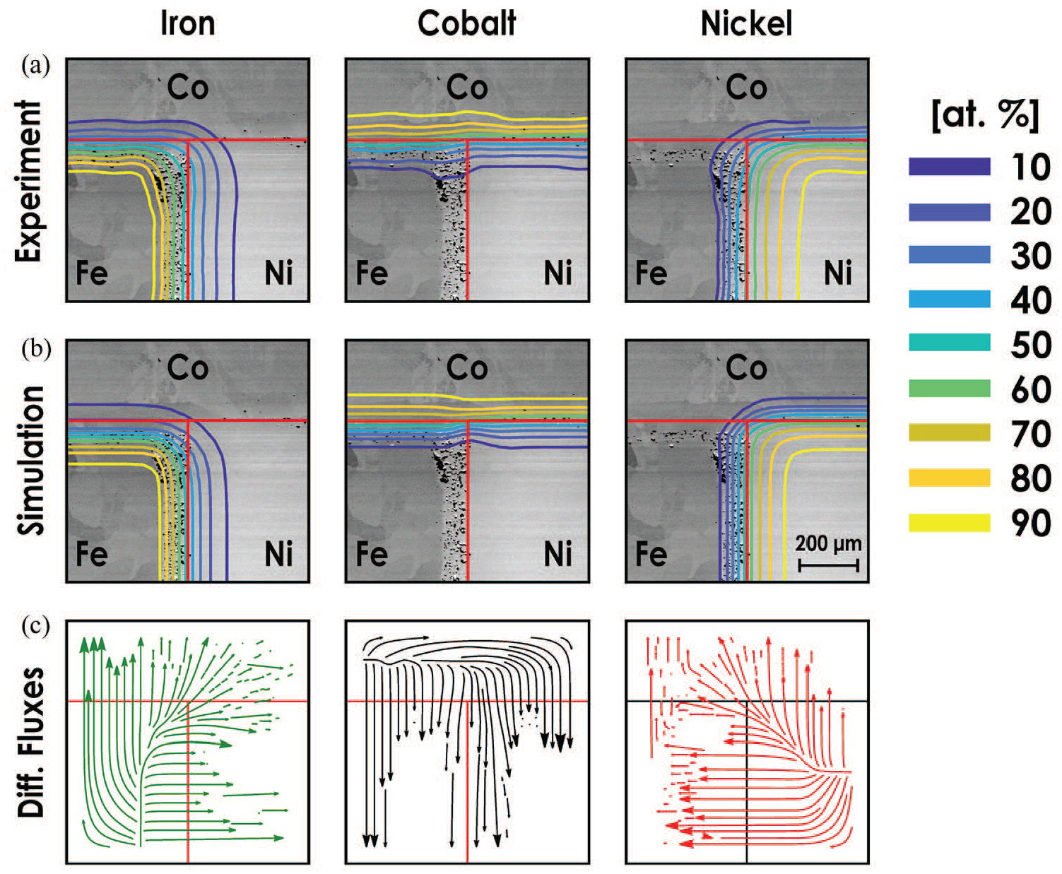
Experimental (a) and simulated (b) concentration maps, and the fluxes (c) in the Fe-Co-Ni multiple after annealing at 1373 K for 200 h.
For better presentation of the effectiveness of the present model, the concentration profiles for various one-dimensional cross-sections were simulated (Figures 4 to 8). In the figures, we compare the experimental with simulated profiles. In simulations, the one- and two-dimensional difference methods were used (Section 3). Generally, a good qualitative agreement of all sets of data is seen.
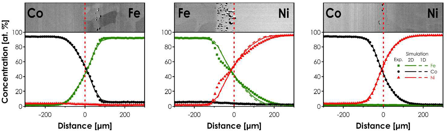
Scanning electron micrographs and concentration profiles at the cross-sections: Fe|Ni, Co|Ni, Co|Fe. The Matano plane position is indicated.
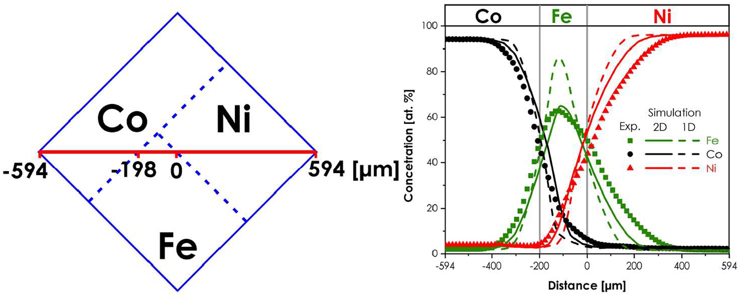
Concentration profiles at the one-dimensional Co|Fe|Ni cross-section (shown on the left) of the multiple.
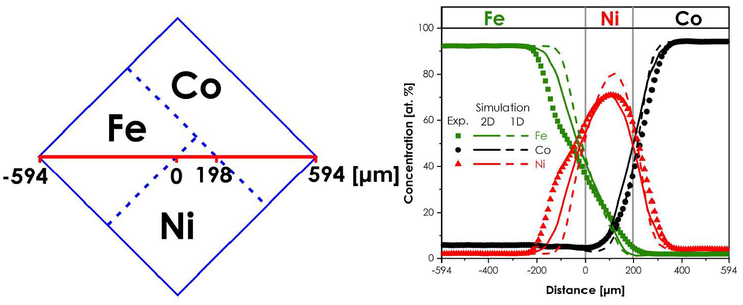
Concentration profiles at the one-dimension Fe|Ni|Co cross-section (shown on the left) of the multiple.
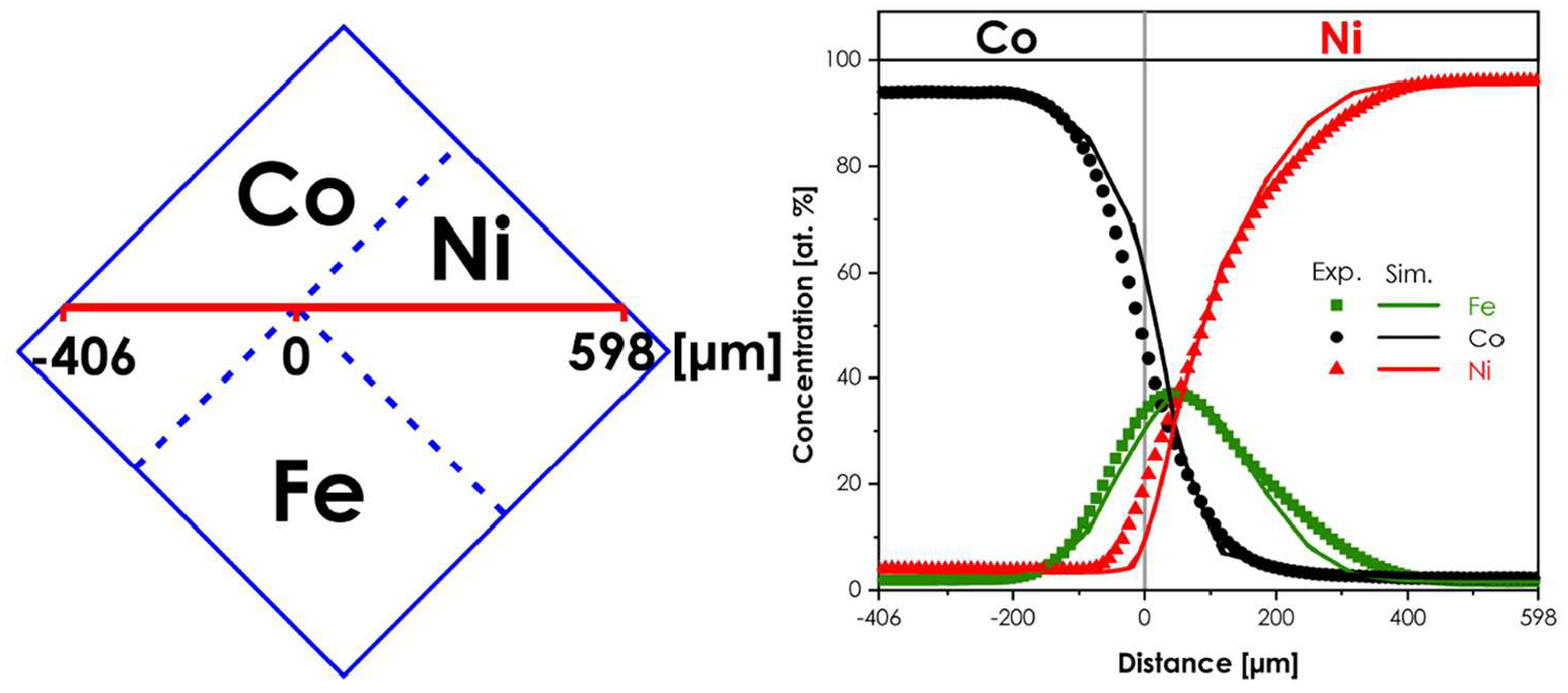
Concentration profiles at the one-dimension Co|Ni cross-section (shown on the left) of the multiple.
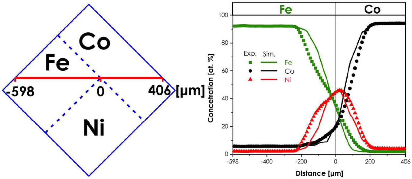
Concentration profiles at the one-dimension Fe|Co cross-section (shown on the left) of the multiple.
In Figure 4, the results for the three pseudo one-dimension couples are shown. We present two sets of simulated data, computed using the one- and two-dimensional methods.
The computed and experimental profiles agree perfectly with experimental data only for the Co|Ni and Co|Fe couples. In the case of the Fe|Ni couple, the data simulated with the one- and two-dimensional models overlap but the experimental results clearly differ. The discrepancy can be attributed to a big fraction of the voids in iron next to the contact plane.
In Figures 5 and 6, we compare the results for the Co|Fe|Ni and Fe|Ni|Co cross-sections passing the three-metal contact point. Here we compare the results from the one- and two-dimensional methods with the experimental ones. For all components, a clearly better agreement with experimental results is provided by the two-dimensional model, which is primarily seen in the case of the central components, Fe and Ni, respectively.
An advantage of the two-dimensional method over the one-dimensional method is particularly seen in Figures 7 and 8, where the concentration profiles at the one-dimensional cross-sections going through the three-metal joint point are shown. Only the two-dimensional method has been used in this case. The one-dimensional model neglects one of the multiple components.
4.2.2. Time evolution
An advantage of any numerical model of the diffusion is that it can be applied to simulate the processing. In Figures 9 to 12, we present the simulations of the time evolution and we show the results for the times
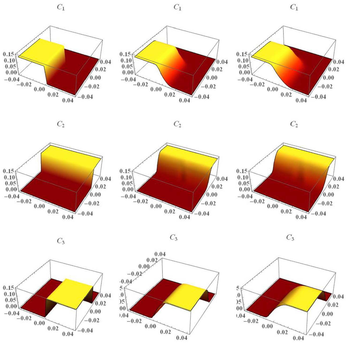
Time evolution of the concentrations of Fe (
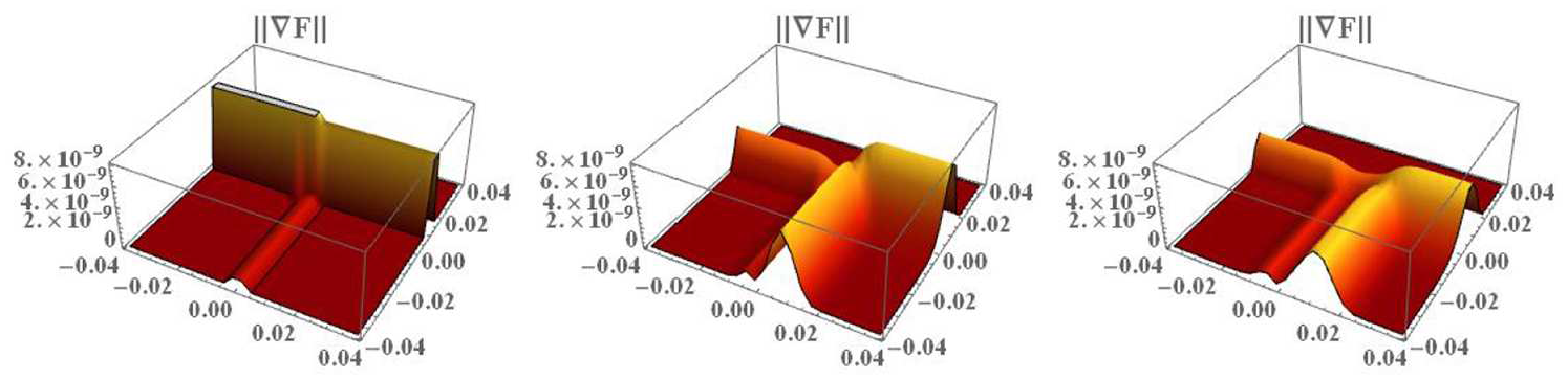
Time evolution of the norm of the drift velocity
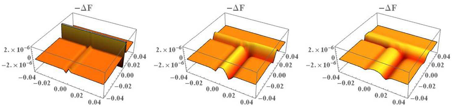
Time evolution of the divergence of the drift velocity div
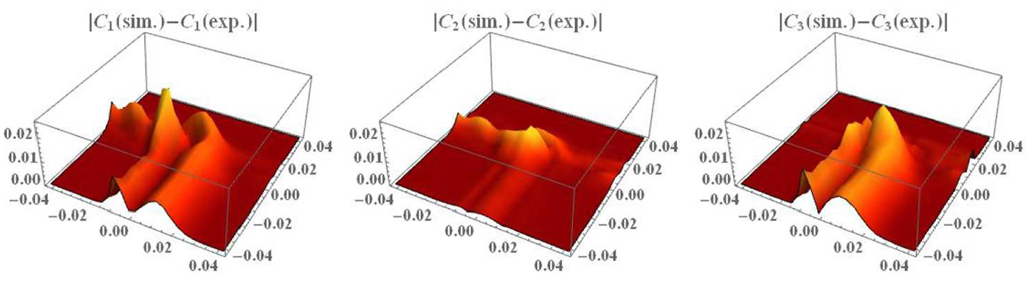
Modules of difference between the experimental and simulated (the last column of Figure 9) concentrations, for 200 h.
5. Conclusions
The results of the paper are summarized as follows:
We presented a theoretical study of the model introduced in [23, 24] of the one- and multidimensional transport in an
The implicit finite difference methods in one and two dimensions were constructed, for the case of nonlinear diffusion coefficients depending on mole fractions. Let us stress that in [24] only the case of constant diffusion coefficients was studied.
The existence and uniqueness of solutions of the implicit difference schemes and consistency of the difference methods were proved. The Vegard rule was preserved.
The numerical results were compared with experimental data for a ternary Fe-Co-Ni system. A good agreement of both sets was revealed, which confirmed a force of the model and numerical methods. The comparison particularly demonstrates that our methods are convergent and stable.
Footnotes
Funding
The author(s) disclosed receipt of the following financial support for the research, authorship, and/or publication of this article: This work was supported by the Faculty of Applied Mathematics AGH UST statutory tasks within subsidy of Ministry of Science and Higher Education (Grant Number 16.16.420.054) and the National Science Centre for OPUS 13 (Grant Number 2017/25/B/ST8/02549).