
Abstract
The vast majority of the roughly half-million elected officials in the U.S. occupy local offices, however, research examining how they get elected to remains scant. The present study examines turnout in local elections, focusing on the effects of electoral rules, the competitiveness of local races, and whether and how place matters. Based on a sample of roughly 10,000 mayoral elections, this study represents the most systematic empirical analysis of local turnout to date. While we find substantial differences in turnout across rural towns, suburbs, and central cities, these differences are largely explained by electoral and contextual factors that are unevenly distributed across the local landscape. Though election timing is far and away the most important factor, uncontested mayoral races, local elections in states with restrictive voting laws as well as those mid-sized municipalities are associated with significantly lower turnout.
One component of a healthy democracy at any level is that its citizens participate in elections, otherwise those who are elected to office may not reflect the interests, values, and beliefs of the population. While we know quite a bit about turnout in federal and state elections, local elections remain much less studied, particularly in the U.S. According to Berry and Howell (2007), less than one percent of the literature on voter turnout focuses on local elections. As a result, we don’t have good answers to even basic questions, such as what percentage of Americans vote for mayors, city councilors, or school board members? There is decent evidence that turnout in big cities tends to be very low (Portland State University 2016), but we know much less about turnout in small- and medium-sized municipalities, the places where the vast majority of Americans live. One reason is because local election data have historically been hard to find, access, and collect. Consequently, empirical studies of turnout in local elections have typically been based on returns that are most readily available, and scholars have tended to focus on samples of cities that are relatively small (Arrington and Ingalls 1984; Gierzynski, Kleppner and Lewis 1998; Krebs 1998; Lieske 1989) and/or limited in scope or geography (Alford and Lee 1968; Caren 2007; Hajnal and Lewis 2003; Holbrook and Weinschenk 2014; Lublin and Tate 1995; Lappie and Marschall 2018; Marschall and Lappie 2018; Wood 2002).
Data issues aside, studies of local elections are theoretically and empirically distinct from the literature on federal and state elections in several important ways. First, rather than relying on information about individual voters, empirical work on local elections tends to employ aggregate-level data (but see Oliver 1999, 2000). Not only is surveying a representative sample of residents in a large sample of local jurisdictions challenging and expensive, but using cities as the unit of analysis makes sense given scholars’ interest in how local electoral and governing arrangements affect turnout. Second, and relatedly, candidate characteristics and features of local campaigns are not nearly as prevalent in studies of local turnout as they are in traditional studies that focus on state and federal elections (but see Holbrook and Weinschenk 2014). The challenges associated with locating and collecting data on local candidates and campaigns help explain why. Finally, while scholars of local elections examine traditional demographic factors, like race/ethnicity, income, and education, they are also interested in contextual and geographic features associated with local jurisdictions. For example, there has been considerable debate in political science about whether and how city size matters for local turnout (Keheller and Lowery 2004, 2009; Oliver 2000), and economists have honed in on the material interests of homeowners to explain the behavior of especially suburban voters or “homevoters” (Fischel 2005). There has also been growing interest among social scientists of all stripes in the ways that ‘sense of place’ might engender civic (and other) attitudes and behaviors (Armstrong and Stedman 2019; Dang et al. 2022; Lappie and Marschall 2018).
Against this backdrop, the current study focuses on three primary research questions. First, how much does variation in local electoral rules, especially election timing, partisan elections, and state laws that restrict voter access explain turnout in local elections? While studies have found that election timing is far and away the most important predictor of turnout in local elections (Hajnal and Lewis 2003; Marschall and Lappie 2018), most of what we know comes from studies of California, where mayoral elections tend to be off-cycle and where cities tend to be relatively large. Second, how much does competition matter? Given that interest in politics is one of the most significant factors in electoral participation (Oliver 2000), it seems likely that the absence of electoral competition would disincentivize turnout. Previous studies have examined how competition, measured by campaign spending, margin of victory, and the number of candidates running, affects local turnout (Holbrook and Weinschenk 2014). While these studies provide valuable insights, they too have tended to focus on larger cities, where unopposed mayoral races are quite rare, rather than small rural and suburban towns, where the absence of contestation is often the norm (see Williams, Marschall and Lappie 2017). Third, does “place,” separately from the demographic or socioeconomic features of a place's inhabitants, matter when it comes to turnout in local elections? Lappie and Marschall (2018) found that turnout in mayoral elections was significantly higher in rural towns than in other types of municipalities. However, it is not clear that their finding holds up outside of the two states they examined (Indiana and Kentucky).
The present study utilizes a sample of some 10,000 mayoral elections from over 2,400 cities located in nine states (LEAP 2017) to examine these questions. In addition, the considerable variation in demographic, contextual, and institutional features of municipalities included in the sample, this study allows us to examine whether existing findings holdup across an expanded set of states and a much larger sample of medium- and small-size cities, which make up the vast majority of municipalities in the U.S. The broader theoretical and empirical scope of this study enables us to draw more valid and reliable conclusions about the state of local elections in the U.S. 1
While there are substantive differences in both turnout and the competitiveness of local elections across the places where Americans live, data from our sample indicate that less than half of eligible voters (43 percent) turnout in any given mayoral election in the U.S. and that nearly half of these races (48 percent) are uncontested. However, findings from our study suggest that solutions that can substantially improve turnout in mayoral elections are within reach. Specifically, we find that turnout is most strongly associated with election laws, namely the timing of elections and state laws that restrict voter access. Thus, by simply shifting local elections so they coincide with presidential elections, turnout in mayoral elections could be increased by some 25 percentage-points. Eliminating state laws that restrict access to voting could boost turnout by an additional two and a half percentage-points. Our study uncovered other factors that had negative effects on turnout in mayoral elections. The first is city size, where we found significant, though non-linear effects. Compared to small towns, mid-sized cities had significantly lower turnout, ranging from 3.5 to about 8 percentage-points on average. On the other hand, turnout in mayoral races was not significantly lower in the largest U.S. cities. We also found that unopposed mayoral races were associated with significantly lower turnout than races featuring two or more candidates. On average, the difference was nine percentage-points.
What We Know About Turnout in Local Elections in the U.S.
The heterogeneity of local places and governments along with data limitations have traditionally made it difficult to describe with any confidence what average turnout in local elections across the U.S. looks like. A recent study of mayoral turnout in the nation's largest thirty cities showed that average turnout was a mere 15 percent of the citizen voting-age population (Jurjevich et al. 2016). However, focusing on the largest cities in the U.S. tends to capture observations concentrated in the left tail of the turnout distribution. Indeed, turnout in municipal elections is not universally low. For instance, in Minnesota turnout in mayoral elections averages over 50 percent, and in cities like Portland, OR or Cranston, RI, turnout is routinely higher than this, and on par with turnout rates for presidential elections. The fact that variation in turnout is so much greater at the local than either the state or federal levels suggests that any effort to explain local turnout cannot rely solely on explanatory factors employed in studies of state and federal elections.
When it comes to theory and approach, studies of local elections are divided between those that rely on individual-level theories and data, and those that focus on institutional and contextual factors and employ aggregate-level data. While the former provide excellent information on the motivations of the individual voter, they generally do not help us understand whether or how electoral rules or the features of cities impact turnout. This in part, is why studies that employ aggregate-level data and treat the local jurisdiction (typically the municipality) as the unit of analysis are most common. Within this body of work, two broad sets of explanatory factors have featured most prominently: electoral rules and features of the local context. 2 Table 1 provides a summary of these studies.
Summary of Key Empirical Studies of Turnout in U.S. Local Elections
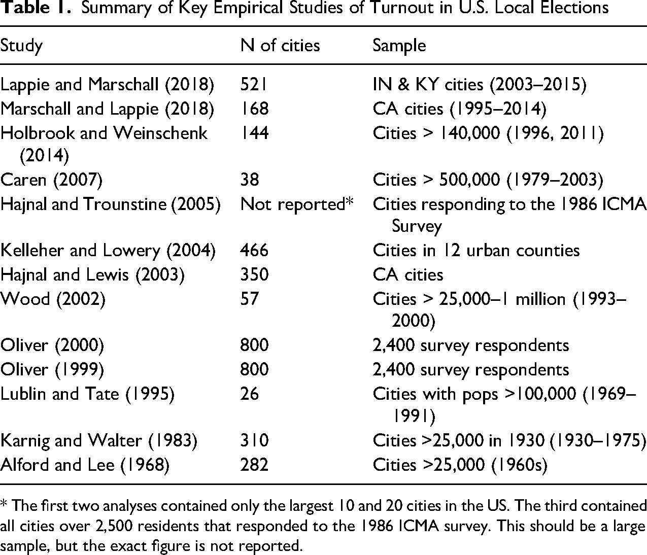
* The first two analyses contained only the largest 10 and 20 cities in the US. The third contained all cities over 2,500 residents that responded to the 1986 ICMA survey. This should be a large sample, but the exact figure is not reported.
Theoretical Framework
Nearly all studies of turnout are rooted in the costs and benefits of participation. The present study focuses on how interest and information in particular can both reduce the costs of voting and increase benefits associated with participating in the electoral process. Our theoretical framework examines how electoral rules, competition, and place shape turnout in local elections by operating on the costs/benefit calculus of would-be voters.
Electoral Rules and Voter Access
Scholarly interest in how electoral rules affect turnout in local elections stems partly from the fact that these rules vary tremendously at the municipal level, and increasingly the state level, and partly because many were introduced with at least an implicit goal of limiting turnout. For example, Progressive Era reformers despised the corrupt and inefficient party machines of the late 19th and early 20th centuries and adopted reforms like the recall, referendum, and initiative, city managers, nonpartisan elections, and off-cycle elections in an effort to weaken and destroy them. Off-cycle elections in particular were meant to separate local politics from national politics, undermining the influence of party machines. However, the progressives also believed that off-cycle local elections would lead to lower turnout rates, particularly among the working-class, and racial/ethnic minorities, who were the backbone of most party machines (Anzia 2014; Trounstine 2008).
Of all the electoral rules examined in empirical research on local elections, election timing is far and away the most influential. 3 Turnout in local elections is presumed to be higher in on-cycle elections because voters interested in national and state politics are brought out to the polls. 4 Their interest in the federal and state offices on the ballot has already made them accept the most obvious costs of voting: registering to vote and going to the polls. While there is clearly roll-off in these elections (Bullock and Dunn 1996), once at the polls, many voters do complete the full ballot and even more cast votes for local races and questions that are of particular salience to them (but see Wattenberg, McAllister and Salvanto 2000). On the other hand, those same voters may not turn out if the election were held off-cycle—due to lower interest, less information, or barriers that make it difficult for voters to get to the polls on multiple days throughout the year. Existing studies have uniformly confirmed these expectations. The seminal study by Hajnal and Lewis (2003) found that half the variance in California's local election turnout was explained by election timing alone, with average turnout in on-cycle municipal elections ranging from 25 to 36 percentage-points higher than those held off-cycle.
In addition to the shift to off-cycle elections, another Progressive Era reform that explicitly targeted ballot access was the nonpartisan election. Designed to remove party cues from the voting calculus, the nonpartisan election caused voters to seek alternative information about candidates and ultimately increased the costs of voting. Nonpartisan elections do not hinder citizens from voting in the election, but rather disincentivize participation. Voters who do not know the names, let alone issue positions, of candidates often rely on party labels as a heuristic (Lau and Redlawsk 2001). In the absence of party labels, citizens may prefer to leave the ballot blank rather than risk voting for the “wrong candidate.” While this presumably depresses voter turnout in general, Progressive Era reformers expected the effect to be particularly strong for low-income, immigrant, and nonwhite voters.
Interestingly, findings on the effects of nonpartisan elections have been somewhat mixed. Early studies found that nonpartisanship was associated with reductions in turnout of around eight percentage-points (Alford and Lee 1968), and that cities adopting nonpartisan elections had greater declines in voter turnout than cities retaining partisan elections (Karnig and Walter 1983). More recent research has typically found no effect of nonpartisanship (Caren 2007; Lublin and Tate 1995; Wood 2002; but see Holbrook and Weinschenk 2014), however most of these studies are based on limited samples. Further, because statewide rules typically determine whether local elections are partisan or nonpartisan, the effects of partisan elections may be difficult to disentangle from state effects.
Apart from Progressive Era reforms, researchers have also considered how contemporary rules and requirements related to voter registration and casting the ballot shape turnout. For example, Caren (2007) looked at variation in how long polls were open across cities in his sample, and Holbrook and Weinschenk (2014) examined whether voter registration deadlines (i.e., the number of days before an election registration closed) mattered for local turnout. Over the past couple of decades states have expanded beyond these more practical and relatively uncontroversial election administration matters by increasingly enacting laws that seek to either increase or restrict voter access. One particularly popular and controversial example is voter ID laws. These laws, which came onto the scene after the 2000 election, place restrictions on the form of ID required, when IDs must be presented, and how voters without the required ID are dealt with at the polls. Similar to voter ID laws, state laws that limit voters’ access to early or absentee voting can prevent eligible voters from successfully casting a ballot. For example, fewer early-voting hours can transfer more pressure onto Election Day resources, leading to longer lines and making voting costlier and more burdensome.
While many states have sought to restrict voter access, others have been doing the opposite. Some notable examples include state laws that make voter registration automatic, the adoption of same-day voter registration, or allowing no excuse absentee (mail-in) voting. In addition, when it comes to felon disenfranchisement, over the last few decades, the general trend has been toward reinstating the right to vote at some point (typically upon release from prison or after probation ends).
In the present study, we test two traditional hypotheses regarding the relationship between electoral rules and turnout in local elections. Specifically, we expect that, all things equal, municipalities with off-cycle or nonpartisan elections will have lower turnout than those with elections held concurrently with presidential or midterm elections, or with ballots featuring partisan labels. Since these tests are based on a larger, more representative sample than those used in previous studies, we expect our analysis to shed important light on just how much election timing, and the lesser studied nonpartisan election, matter for turnout in local elections. In addition to these two hypotheses, the broader, multi-state sample allows us to test for whether a more contemporary set of restrictive voting laws implemented by states (voter ID laws, limited or no early voting, and felon disenfranchisement) is associated with turnout in local elections.
Competition and Local Elections
As one might expect, competitive elections are associated with greater media attention, campaign spending, and voter interest. While less studied at the local level, Holbrook and Weinschenk (2014) provide the most comprehensive and definitive analysis of the effects of competition on turnout in local elections. Their findings tend to corroborate evidence from federal and state elections showing that competition is associated with higher turnout (Cox and Munger 1989; Hill and Leighley 1999). In particular, they find that campaign spending (logged) had a positive effect on turnout and that the closeness of the race, measured as the margin of victory between the first and second place candidates, also increased turnout (see also Caren 2007). While not looking at turnout, Adams (2018) found that campaign contributions were positively associated with candidates’ vote shares.
The number of candidates vying for office is another indicator of competitiveness. More candidates running suggests greater interest in local politics among a potentially wider array of groups within the city, which in turn could help bolster turnout. On the other hand, a race with a single candidate is by definition uncompetitive. Such races may suggest a lack of interest in running for or holding office or in local politics more generally or belief among would-be candidates that their chances of winning are too low. Further, candidates who run unopposed have little incentive to mobilize voters, while voters have little incentive to vote in an election where they have no choices to make. While studies find limited support that the number of candidates competing for office affects turnout (Hajnal, Lewis and Louch 2002; Holbrook and Weinschenk 2014; Norrander 1986), there is strong, consistent evidence that uncontested races are associated with lower turnout (Aldag 2019; Hajnal, Lewis and Louch 2002; Lappie and Marschall 2018).
The presence of incumbents on the ballot is yet another indicator of electoral competition. Although the name recognition, fund-raising capacity, and electoral benefits enjoyed by incumbents are thought to reduce some costs associated with low salience elections, races that feature incumbents also tend to be less competitive. This is because incumbent candidates often discourage would-be challengers from running (Jacobson and Kernell 1983). When challengers do emerge, incumbents’ significant electoral advantages can often make the race less interesting to voters, thereby reducing turnout. By and large, empirical studies of local elections have found little to no effect of incumbency on turnout (Hajnal, Lewis and Louch 2002; Holbrook and Weinschenk 2014; Lappie and Marschall 2018). 5 This may be because these studies also control for uncontested races or the number of candidates running, or because they are based on samples that only include larger U.S. cities. The present study tests for the relationship between uncontested mayoral races as well as mayoral contests that feature incumbents. Ceteris paribus, we expect both to be associated with lower turnout compared to contests with at least one challenger or an open seat.
Place and the Local Context
In addition to electoral rules and the competitiveness of local contests, studies of turnout have found that where and how voters live matters. For example, although not looking at local elections, Wolfinger and Rosenstone (1980) found that people who live in rural areas are more likely than those who live in urban areas to vote. In fact, research on turnout in local elections has focused considerable attention on how city size and a variety of city-level demographic and socio-economic characteristics shape residents’ participation. This research examines how factors like population size and density, household income and inequality, race/ethnicity, and homeownership shape political behavior at the local level (Books and Prysby 1991; Huckfeldt 1986; Oliver 1999, 2000). Generally, these contextual features have been conceptualized and measured as aggregations of the individuals who reside in local jurisdictions, rather than features of the places themselves. Hypothesized causal mechanisms linking contextual features to behavioral outcomes in these studies include the psychological effects of living in dense, large, or poor areas (e.g., via anomie or threat), the social structures, processes, and interactions that shape information flows, resources, interest, and opportunities for participation, or the norms, sanctions, and social pressures surrounding political activism. Thus, it is the characteristics of local inhabitants rather than something about the place itself that is associated with variation in turnout across jurisdictions.
A recent study by Lappie and Marschall (2018) argued that the spatial, geographic, and functional features of places might themselves shape turnout. They focused on city type, which in the U.S. is commonly defined as central cities, suburbs, and rural towns. Central cities are located in metropolitan areas and represent the economic and social center of these relatively large and more densely populated areas. Suburbs are incorporated municipalities that are located in a metropolitan area, but are simply in the economic and (typically) social orbit of a nearby central city rather than serving this function themselves. Finally, rural towns are located outside metropolitan areas and tend to be geographically, economically, and socially distinct from both central cities and suburbs.
In many ways, rural towns embody what Verba and Nie (1972) called bounded communities. Because they are relatively isolated and usually do not directly border other municipalities, there is a clear distinction between town and countryside. Residents in rural towns are likely to perform their economic and social activities within town limits. Since nodes of human activity tend to generate greater interest/attachment to particular places (Agnew 1987), this may help explain the positive relationship between rural residence and higher turnout (Wolfinger and Rosenstone 1980). Conversely, suburbs generally lack clear boundaries (Verba and Nie 1972), and suburbanites are just as likely, if not more likely, to perform their economic and social activities in other suburbs (or the central city) as they are in their hometown. The lack of clear demarcation between a suburb and similar communities, and the proximity to the central city, may make it difficult for suburban residents to consider their municipality as distinct and important. Finally, similar to suburbs, central cities are not geographically isolated. While we posited that this would have a negative effect on turnout in suburbs, we believe the effect for central cities is weaker because they are larger, more diverse, and provide more outlets for human activity than the surrounding suburbs. Furthermore, since central cities typically offer more government services than suburbs, city government is more visible and thus likely to be more important to the lives of its residents.
Overall, the geographic, spatial, and functional features of U.S. cities work together to make municipalities more (or less) salient and meaningful in the lives of their residents. Controlling for demographic, contextual, and institutional features, we expect suburbs to have the lowest turnout rates, rural towns the highest, and central cities somewhere in between.
Data and Methods
We test the hypotheses developed above on a dataset of approximately 10,000 mayoral elections held across nine states between 2000 and 2017 (LEAP 2017). This dataset contains cities of all sizes, from tiny Funkley, Minnesota (population 5) to Los Angeles, the nation's second largest city. 6 Table 2 presents a breakdown of municipalities (cities, towns, villages) in the sample compared to the U.S. population (in 2019). Municipalities in the nine states vary greatly in terms of geography, socio-demographic characteristics, governmental and electoral arrangements. This variation allows a more robust empirical analysis of the determinants of turnout in mayoral elections and makes the results more generalizable. Table 3 reports the number of observations, available years, method, and timing of elections by state. 7
Sample and Population Municipalities by Size
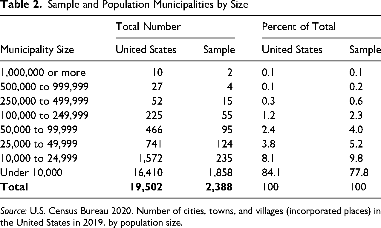
Source: U.S. Census Bureau 2020. Number of cities, towns, and villages (incorporated places) in the United States in 2019, by population size.
Sample Characteristics
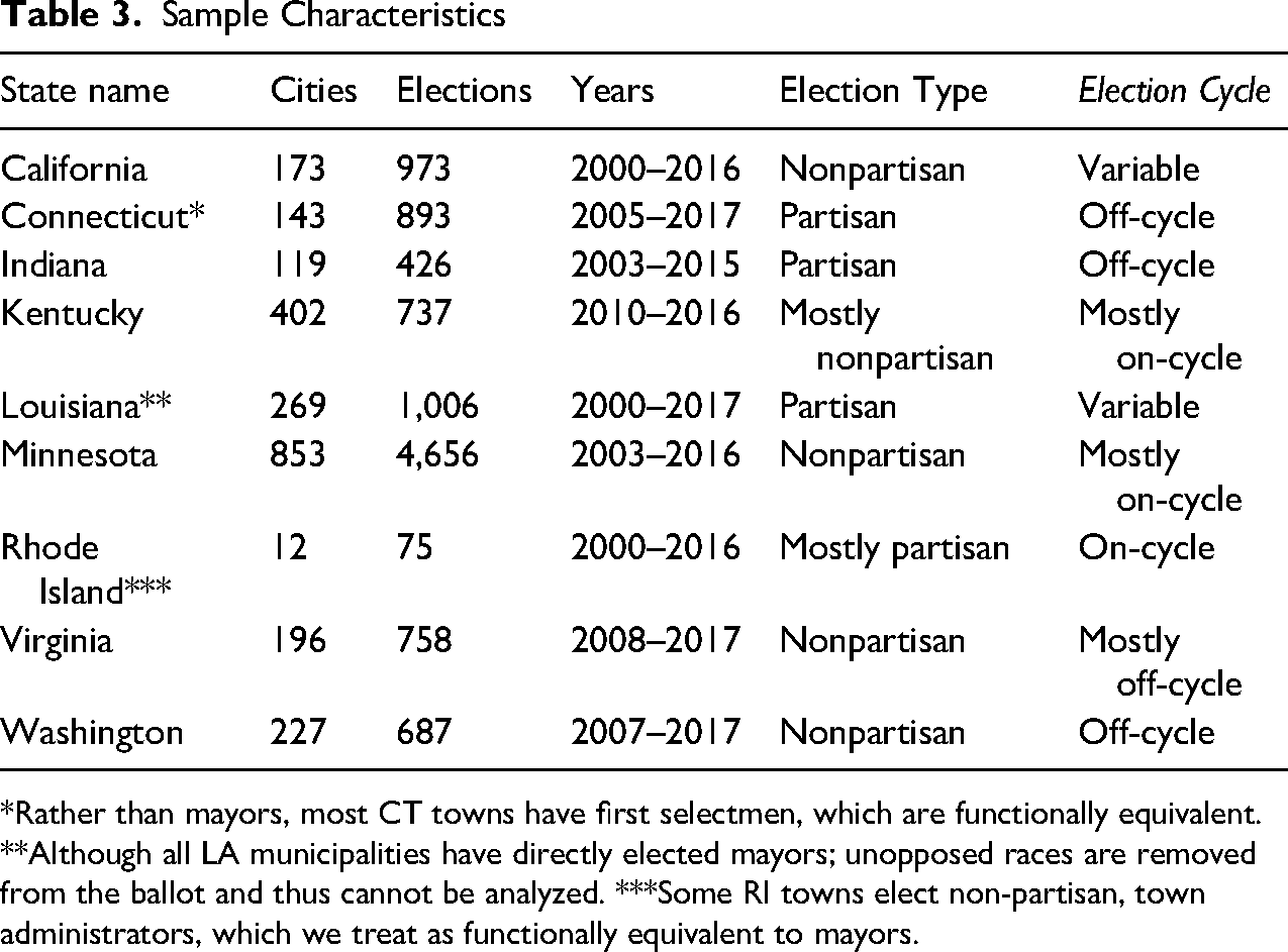
Rather than mayors, most CT towns have first selectmen, which are functionally equivalent. **Although all LA municipalities have directly elected mayors; unopposed races are removed from the ballot and thus cannot be analyzed. ***Some RI towns elect non-partisan, town administrators, which we treat as functionally equivalent to mayors.
Note that the vast majority of municipal elections in our sample (98 percent) represent the contest that produced the winner. This is typically the ‘general’ election, though in Louisiana, which has open or ‘jungle’ primaries, winners are almost always determined in the primary rather than the general election. In two states with mixed election timing (California and Louisiana), we included a small number of first stage elections that did not produce a winner because these were the ‘regularly’ scheduled elections. 8 While there could be some missing races based on the state or county source data, our sample includes all mayoral elections for which local election results were publicly available in the nine states between 2000–2017.
Demographic data for municipalities comes from two U.S. Census Bureau products: the 2000 U.S. Census and the American Community Survey (ACS) 5-Year Data (2012–19). 9 Since the Census Bureau moved many key variables to the ACS after 2000, we use the ACS data from 2010 onward. Since the unit of analysis is a city-year, we employ linear interpolation to estimate values for years between 2000 and 2010, when annual ACS data were not available.
Variables and Measurement
Our dependent variable is the percentage of the voting age population (VAP) casting a ballot for the office of mayor in each election. We use VAP rather than citizen voting-age population (CVAP) because the latter is not available at the municipal level in the 2000 Census and thus cannot be used to interpolate for years for which the ACS did not yet exist. 10 We divide the total number of votes for mayor by the total number of municipal residents aged 18 and above (VAP).
We include three different variables to measure electoral rules. Foremost among these is election timing, where we use a series of dummy variables: 1 if the mayoral election was held simultaneously with a presidential (Presidential) or midterm general election (Midterm), 0 if not. Elections held on dates other than a presidential or midterm general election are treated as Off-cycle, which is the excluded category. 11 Our second measure denotes the use of partisan elections (1 if party labels appear on the ballot in municipal elections, 0 otherwise). Finally, we include an index that taps the general restrictiveness of state voting laws, focusing here on three laws in particular: early voting, voter ID, and felon (dis)enfranchisement. The index ranges from 0 to 3, varies by state and year, and is based on data reported by the Election Assistance Commission (EAC, various years). 12 Higher values represent more restrictive voting laws. We also test for individual effects of these three laws, though findings here should be treated as suggestive since our study was not designed with these tests in mind. We expect turnout to be higher in municipalities with partisan or on-cycle elections and in states scoring lower on the voting restriction index, all things equal. Our model also includes two variables that tap electoral competition: unopposed mayoral races and contests featuring incumbents (1 if yes; 0 otherwise). 13 We expect mayoral contests with challengers or without incumbents to have higher turnout than uncontested races or contests with incumbents.
We measure city type with a pair of dummy variables for central and suburban cities (rural towns are the excluded category). These classifications are based on 2000 Census. We expect rural municipalities will have the highest turnout rates, with suburban cities having the lowest turnout rates and central cities in-between. In addition to our variables measuring city types, we include a set of control variables that tap socio-economic and other features of the local context. The first is a measure of metropolitan fragmentation that controls for the number of local governments in the county. Number of local governments is the total number of municipal and special district governments (including school districts) located in the county, based on the 2010 U.S. Census of Governments. We constructed the variables based on quartiles, with 0 representing municipalities in the first quartile and 3 corresponding to those in the 4th. In places where there are more governments and more overlapping service jurisdictions, the functional responsibilities of municipalities may be blurred, and the municipality may be less identifiable and of less import to residents. We also include a set of dummy variables for city size. Given the greater range of city sizes our sample, we can test for potential non-linear effects in the relationship between city size and turnout. Along with population size, we also include a measure of the municipality's population density (1,000 s).
There is also a vector of other controls that tap socio-economic characteristics of the municipal population. These include educational attainment (measured as the percent over age 25 with at least a bachelors’ degree), the percentage of the municipality's nonwhite and 65 and older population, the percentage of homeowners and the percentage of both non-citizens and families with school-aged children. We also include a measure of the age of the housing stock, since the architecture of newer housing developments tends to inhibit rather than promote interaction with one's neighbors (Oliver 2001) and may thereby reduce residents’ interest in and information about local politics, driving down turnout. Since residents in so called ‘bedroom communities’—places where many if not most residents commute to a job in a different locality—may also be less interested in and informed about local politics simply because they spend so much time in a different city and in their cars (Langdon 1994), we include a measure for the percentage of residents who spend more than 30 min per day commuting to work. Finally, municipalities that have experienced recent population growth (measured as the percent change in the population over a ten-year period) have a larger number of newcomers who may lack strong ties to the locality, which may depress mayoral turnout (Oliver 2001).
Finally, we include election cycle dummy variables, with the first election cycle in the municipality's time series as the excluded categories respectively, and in some of the models, state dummies (with California as the reference). 14 In Table 4 we report descriptive statistics for the full sample, and, to highlight variation across local jurisdiction, by each of the place types.
Sample Summary Statistics
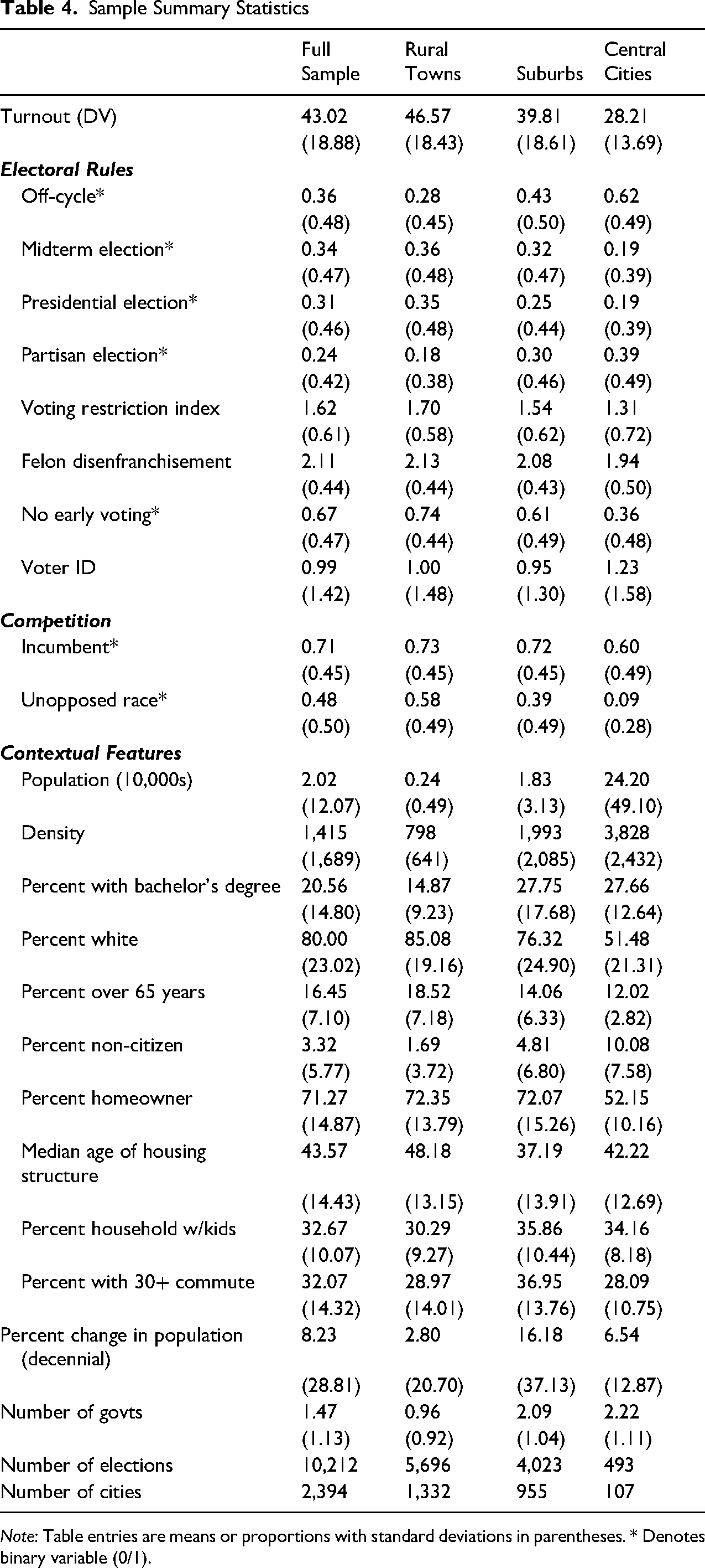
Note: Table entries are means or proportions with standard deviations in parentheses. * Denotes binary variable (0/1).
Empirical Results
We estimate our models using Generalized Least Squares (GLS) regression, with random effects since cities repeat in the dataset, and observations are thus not independent of one another. Failing to account for this would lead to inefficient standard errors. As an additional robustness check, we estimate robust standard errors clustered on the municipality. The coefficients can be interpreted as the marginal effect of a one unit change in the independent variable on turnout, ceteris paribus. We estimate three different models with progressively more control variables (Table 5). The first model includes our key independent variables of interest: those measuring electoral rules (election timing, partisan elections, and the index of state voting restrictions), competition (incumbency and unopposed races), 15 and the city type dummies. Controls for the election cycle are also included in this, and all other models. This model provides an important starting point for comparison and illustrates just how important the inclusion of other control variables and the state dummies will be. Model 2 includes the full set of control variables and Model 3 adds the state dummies. 16
GLS Regression Results
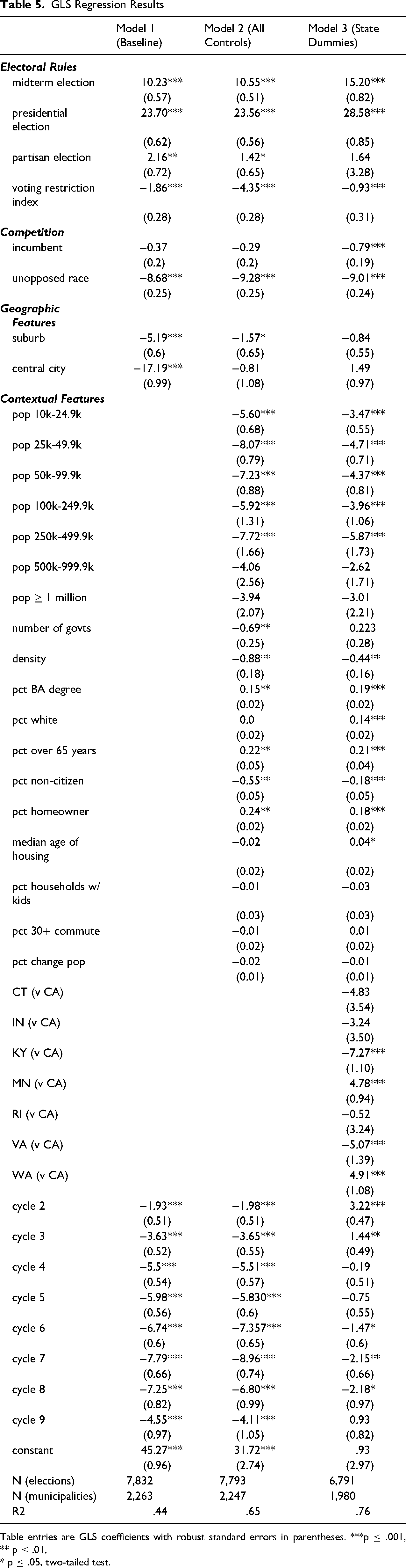
Table entries are GLS coefficients with robust standard errors in parentheses. ***p
* p
There are two important takeaways from this model building exercise. First, the effects of election timing are substantial and are only slightly affected by the inclusion of control variables and state dummies. Second, the effects of several variables, city type and partisan elections in particular, are also quite sizeable; however, once the full set of control variables is included, their effects are greatly attenuated. This underscores the diversity of state and local contexts in the U.S., the value of a large, representative sample, and the importance of control variables. From here, we shift our focus to the estimates from Models 2 (all controls) and 3 (all control variables plus state dummies) and Figure 1, which displays the coefficient plot for our key independent variables from these two models.
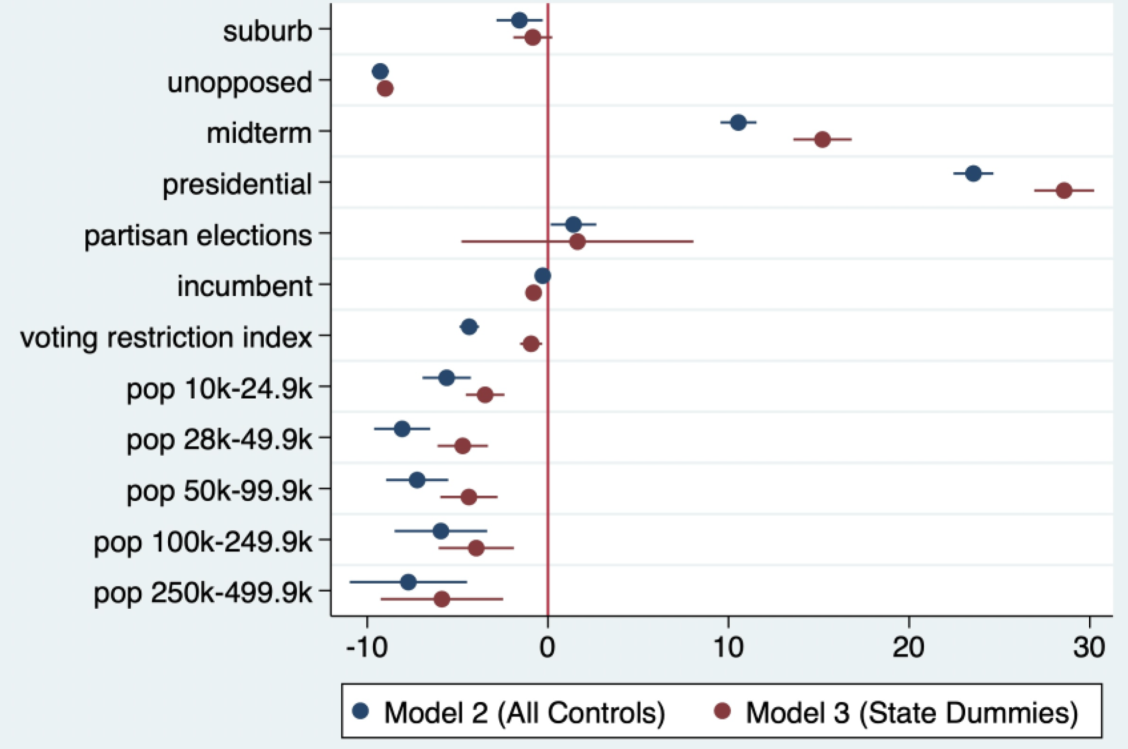
Coefficient plot.
What is abundantly clear in the coefficient plot depicted in Figure 1 is the magnitude of the election timing effect. All things equal, municipalities that hold mayoral elections concurrently with presidential elections see average turnout between 24 and 29 percentage-points higher than municipalities that hold mayoral elections off-cycle. Municipalities whose mayoral elections are held concurrently with midterm elections also see significantly higher turnout—between 11 and 15 percentage-points.
While the effects of election timing are not attenuated by the inclusion of the full set of controls or the state dummies, this is not the case for the effects of partisan elections, and to a lesser extent, the index measuring the three state voter access laws. This is perhaps not surprising given the partisan election variable is binary and since there is little within state variation. 17 This makes disentangling the effects of partisan elections and the state dummies more difficult. In Model 2, partisan elections are associated with a nearly 1.5 percentage-point increase in turnout, however, in Model 3 the coefficient loses its statistical significance. In contrast, the coefficient for the voting restriction index more than doubles in size in Model 2. Controlling for city size and other demographic and contextual factors, state laws that restrict voting access are associated with significantly lower turnout (about 13 percentage points for elections in states with the most to the least restrictive voting laws). While the coefficient remains significant in Model 3 (state dummies), the magnitude of the effect is greatly reduced. This is a tough test given that the voting restrictions analyzed here did not change in four of the nine states between 2000 and 2017. Nevertheless, our findings indicate that municipalities in the state scoring highest on the voting restriction index (VA), have turnout rates that average about two and half percentage points lower than municipalities in states that score the lowest (CA and MN).
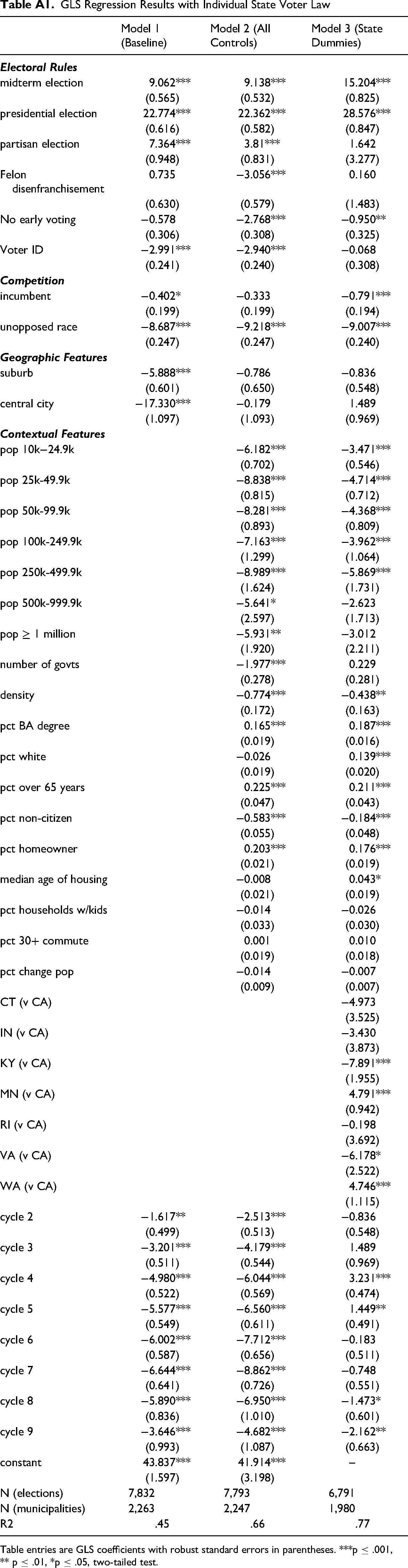
The non-trivial effect of the voting restriction index naturally leads to the question of how the component parts of the index—felon disenfranchisement, voter ID laws, and the absence of early voting—are individually related to turnout. To explore this question, we ran the same three models from Table 5 substituting the voting restriction index with the individual measures of the three specific state laws. The full models are reported in Table A1 in the Appendix. Figure 2 displays the coefficient plot for the three individual measures.
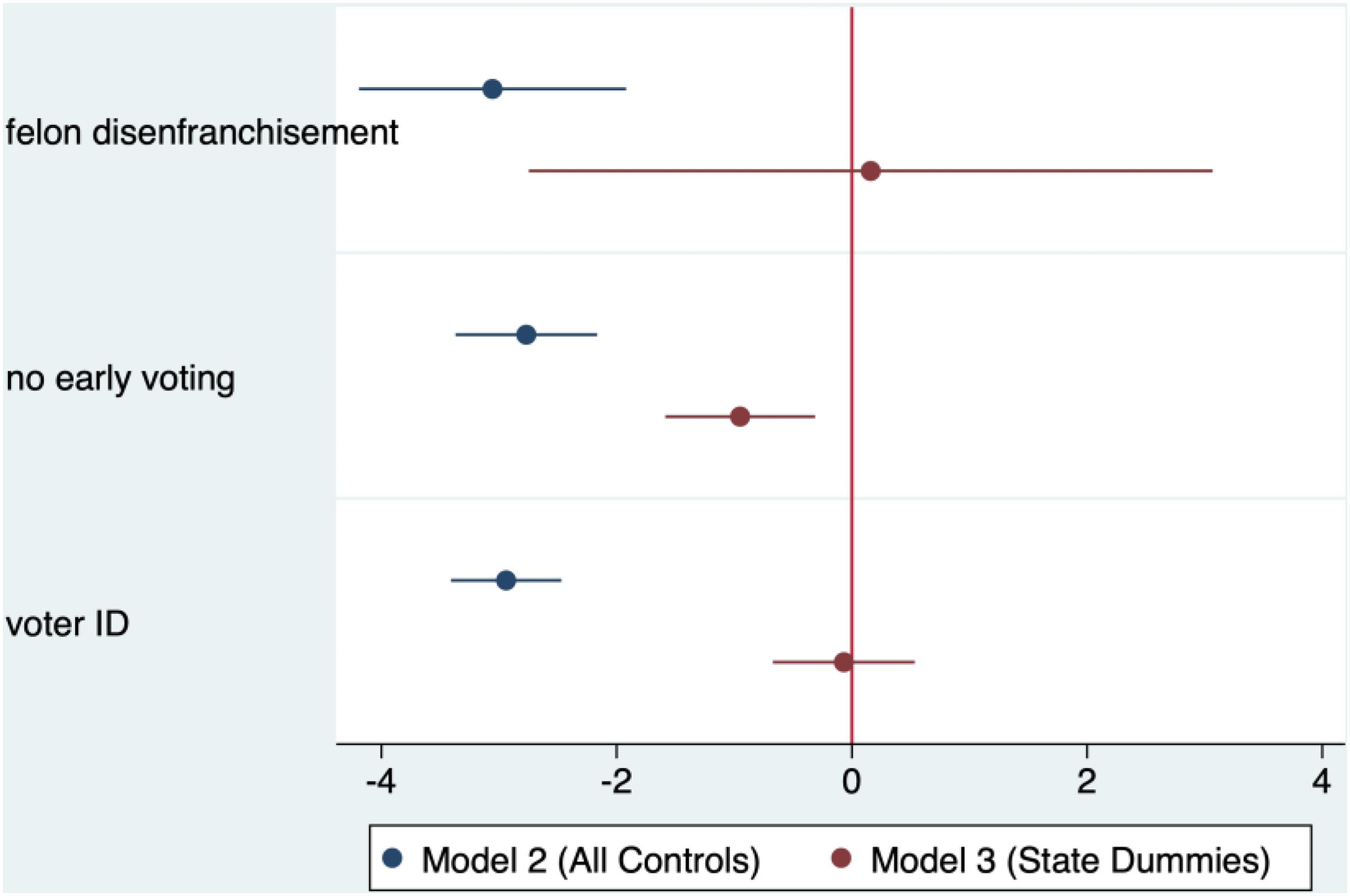
Coefficient plot for voting restriction measures.
As the coefficient plot indicates, the individual measures are statistically significant in Model 2. For each, a one-unit increase (more restrictive) corresponds to about a three percentage-point decrease in turnout. However, when the state dummy variables are included (Model 3), only the variable measuring the absence of laws allowing early voting remains statistically significant. Since this is a binary measure, it indicates that municipalities in states without access to early voting see about a one percentage-point decrease in turnout compared to municipalities in states with early voting. While these findings clearly demonstrate that state voting laws matter for turnout in local elections, we recommend additional analysis, ideally with research designs that are explicitly intended to test for these effects.
Shifting attention back to Table 5 and Figure 1, we can see that electoral rules and voter access are not the only covariates that are strongly associated with turnout. Competition also matters. In particular, mayoral races that feature at least two candidates see significantly higher turnout than those with uncontested races. Across all three model specifications, the effect of an uncontested mayoral race translates into about a nine percentage-point decrease in turnout. Electoral competition is also reduced by the presence an incumbent mayor on the ballot. Our results indicate that while races with incumbents are associated with lower turnout, the effect is relatively minor—about one percentage-point on average (Model 3).
The coefficient plot in Figure 1 also reveals that the inclusion of the full set of control variables has not completely washed away the effect of city type. While there is no statistically significant, independent effect for central cities, there is a statistically significant and negative effect for suburban jurisdictions. Compared to rural towns, turnout in suburbs is about one and a half percentage-points lower, on average (Model 2). This result confirms Lappie and Marschall (2018), who found higher turnout in rural towns versus suburbs in Indiana and Kentucky. In addition, Figure 1 shows that city size has statistically and substantively significant effects on turnout, though not exactly as the literature might have expected. It appears that the more heterogenous sample of municipalities, particularly regarding municipal populations, allowed for a broader test of the effect of city size than many prior studies. Our findings indicate that city size is not linearly related to turnout, but that instead, only in mid-sized cities does turnout significantly differ. Specifically, compared to small towns (those under 10,000), turnout in mid-sized cities is between 3.5 and 8 percentage-points lower. On the other hand, in the largest U.S. cities, those over 500,000, turnout in mayoral elections are not significantly different than in the smallest U.S. towns.
Finally, our empirical findings indicate that many of the variables tapping socio-demographic features of municipalities matter. In particular, municipalities with higher percentages of college educated residents, homeowners, non-Hispanic Whites, and senior citizens have significantly higher turnout rates, as do cities with older housing stocks. On the other hand, municipalities with larger shares of non-citizens and with higher density have significantly lower turnout. These effects are not reported in the coefficient plot (Figure 1), however, for many variables a one percentage-point change is associated with between a 0.1 and 0.2 percentage-point change in turnout (Model 3). When we consider this across a one standard deviation change in the independent variable, it typically corresponds to about a four to six percentage-point change in turnout. For example, all things equal, cities where 35 percent of residents are over 65 years of age see turnout rates averaging five and half percentage-points higher than cities where only five percent of residents are seniors. Similarly, compared to cities where only half of residents are homeowners, in those where 85 percent of residents own their own home turnout is also about five and a half percentage-points higher.
Discussion and Implications
Judging by rates of turnout and contestation in mayoral races across the roughly 2,500 municipalities examined in this study, it seems safe to conclude that there is room for improvement when it comes to the health of local elections in the United States. While turnout varies considerably, across the more than 10,000 mayoral races we investigated, it averaged only 43 percent, and almost half of all races (48 percent) were unopposed. Though these statistics seem rather pessimistic, our study confirms prior research, which finds that the most powerful predictor of turnout in mayoral elections is when the election is held (Hajnal and Lewis 2003; Marschall and Lappie 2018). We find that irrespective of size or location, municipalities with off-cycle elections have turnout rates about 25 percentage-points lower than municipalities whose mayoral elections are concurrent with presidential elections. The good news then, is that a very promising means by which to significantly increase turnout in local elections is not only quite simple, but also clearly within the province of policymakers: changing the election date.
Our study of turnout in local elections also shed important new empirical light on the effects of city size. With the larger and more diverse sample of localities employed in this study, we found significant, though non-linear effects of city size on turnout in mayoral races. Compared to the smallest towns, medium-sized cities have significantly lower turnout, ranging from about 3.5 to 8 percent-points on average. In contrast, we found no difference in turnout between the biggest cities and these small towns.
Beyond the effects of election timing and city size, this study broke new ground as well. In particular, we looked at how election laws, namely partisan elections and state laws seeking to restrict voting access, shape turnout in mayoral elections. While we uncovered evidence that both matter for local turnout, effect sizes were attenuated with the introduction of state dummy variables. However, the statistically significant effects of the voting restriction index remained. Municipalities in states that scored highest on the index of state voting restrictions saw significantly lower turnout rates (about 2.5 percentage-points) than those in states with the least restrictive laws. When we looked at the component parts of this index separately, our findings suggest that all three laws, those prohibiting early voting, requiring government-issued photo IDs to vote, and disenfranchising felons, operate independently on local turnout. This preliminary evidence indicates that these “Jim Crow 2.0” laws are associated with significantly lower turnout at the local level, suggesting that further exploration and analysis are warranted. Indeed, the number and type of other restrictive voting laws is on the rise (Brennan Center for Justice 2021), and we do not know what, if any, additional impact these laws have on local turnout. It is possible that restrictive laws operate even more strongly on turnout in off-cycle elections or in municipalities with larger shares of low-income or minority voters. After all, in presidential and midterm years parties, candidates, and civic-minded NGOs exert a great deal of effort telling voters what forms of voter ID are acceptable, how to cast provisional ballots, when registration and early voting deadlines are, etc. These things are less likely to occur in off-cycle elections for local office, where campaigns are typically much more limited, and where parties are often uninvolved. In addition, since some laws disproportionately affect low-income and minority voters, who already face greater barriers, there is good reason to believe that the effects of these Jim Crow 2.0 laws may be felt more strongly in municipalities where these voters are more concentrated. Future studies could fruitfully explore these and other questions.
Finally, while existing research has examined the relationship between competition and turnout, typically finding that more competition leads to higher turnout, few studies have focused on the other extreme: the lack of any competition at all. In this study, we took a closer look at how unopposed mayoral races affect turnout. Our results show that these races are associated with significantly lower turnout than those with two or more candidates. In fact, turnout in these races was on average nine percentage-points lower than turnout in contested mayoral races. This effect is large enough to nearly wipe out the boost in turnout associated with holding mayoral elections concurrently with midterm elections. The role of contestation and the impact of unopposed elections on local turnout are substantial and deserve more scholarly attention.
In sum, our study makes a number of important contributions to the literature on local elections. Having access to a dataset that included a representative sample of municipalities in the U.S. provided greater variance in many key variables, including election timing, partisan elections, city size, and importantly, contestation, thereby enabling us test for how both traditional and more novel factors shape turnout in local elections. At the same time, the data allowed for some important descriptive insights about the state of local elections in the U.S. For example, while the vast majority of Americans live in medium- and small-sized cities, these are the places prior research has studied least. Our data revealed that it is actually in America's smallest towns, which make up 84 percent of all municipalities in the U.S., where turnout in mayoral elections is highest. At the same time, uncontested elections are most common in these small towns. Fully 56 percent of mayoral candidates in small towns ran unopposed. This compares to only eight percent of mayoral races in large cities and 22 percent of mayoral races in medium-sized cities. Importantly, our study also found that independent of city size and a host of other variables controlling for socio-demographic and institutional features, there are significant differences in turnout across rural and suburban municipalities. While the broader scope of the present study allowed us to take a closer look at the state of local elections in the places where most Americans live, clearly even more work is needed to better understand how electoral access, competition, and place shape turnout across the diverse, local landscape of the U.S.
Footnotes
Declaration of Conflicting Interests
The authors declared no potential conflicts of interest with respect to the research, authorship, and/or publication of this article.
Funding
The authors received no financial support for the research, authorship, and/or publication of this article.
Notes
Author Biographies
Appendix
GLS Regression Results with Individual State Voter Law
| Model 1 (Baseline) | Model 2 (All Controls) | Model 3 (State Dummies) | |
|---|---|---|---|
|
|
|||
| midterm election | 9.062*** | 9.138*** | 15.204*** |
| (0.565) | (0.532) | (0.825) | |
| presidential election | 22.774*** | 22.362*** | 28.576*** |
| (0.616) | (0.582) | (0.847) | |
| partisan election | 7.364*** | 3.81*** | 1.642 |
| (0.948) | (0.831) | (3.277) | |
| Felon disenfranchisement | 0.735 | −3.056*** | 0.160 |
| (0.630) | (0.579) | (1.483) | |
| No early voting | −0.578 | −2.768*** | −0.950** |
| (0.306) | (0.308) | (0.325) | |
| Voter ID | −2.991*** | −2.940*** | −0.068 |
| (0.241) | (0.240) | (0.308) | |
|
|
|
||
| incumbent | −0.402* | −0.333 | −0.791*** |
| (0.199) | (0.199) | (0.194) | |
| unopposed race | −8.687*** | −9.218*** | −9.007*** |
| (0.247) | (0.247) | (0.240) | |
|
|
|||
| suburb | −5.888*** | −0.786 | −0.836 |
| (0.601) | (0.650) | (0.548) | |
| central city | −17.330*** | −0.179 | 1.489 |
| (1.097) | (1.093) | (0.969) | |
|
|
|||
| pop 10k−24.9k | −6.182*** | −3.471*** | |
| (0.702) | (0.546) | ||
| pop 25k-49.9k | −8.838*** | −4.714*** | |
| (0.815) | (0.712) | ||
| pop 50k-99.9k | −8.281*** | −4.368*** | |
| (0.893) | (0.809) | ||
| pop 100k-249.9k | −7.163*** | −3.962*** | |
| (1.299) | (1.064) | ||
| pop 250k-499.9k | −8.989*** | −5.869*** | |
| (1.624) | (1.731) | ||
| pop 500k-999.9k | −5.641* | −2.623 | |
| (2.597) | (1.713) | ||
| pop ≥ 1 million | −5.931** | −3.012 | |
| (1.920) | (2.211) | ||
| number of govts | −1.977*** | 0.229 | |
| (0.278) | (0.281) | ||
| density | −0.774*** | −0.438** | |
| (0.172) | (0.163) | ||
| pct BA degree | 0.165*** | 0.187*** | |
| (0.019) | (0.016) | ||
| pct white | −0.026 | 0.139*** | |
| (0.019) | (0.020) | ||
| pct over 65 years | 0.225*** | 0.211*** | |
| (0.047) | (0.043) | ||
| pct non-citizen | −0.583*** | −0.184*** | |
| (0.055) | (0.048) | ||
| pct homeowner | 0.203*** | 0.176*** | |
| (0.021) | (0.019) | ||
| median age of housing | −0.008 | 0.043* | |
| (0.021) | (0.019) | ||
| pct households w/kids | −0.014 | −0.026 | |
| (0.033) | (0.030) | ||
| pct 30+ commute | 0.001 | 0.010 | |
| (0.019) | (0.018) | ||
| pct change pop | −0.014 | −0.007 | |
| (0.009) | (0.007) | ||
| CT (v CA) | −4.973 | ||
| (3.525) | |||
| IN (v CA) | −3.430 | ||
| (3.873) | |||
| KY (v CA) | −7.891*** | ||
| (1.955) | |||
| MN (v CA) | 4.791*** | ||
| (0.942) | |||
| RI (v CA) | −0.198 | ||
| (3.692) | |||
| VA (v CA) | −6.178* | ||
| (2.522) | |||
| WA (v CA) | 4.746*** | ||
| (1.115) | |||
| cycle 2 | −1.617** | −2.513*** | −0.836 |
| (0.499) | (0.513) | (0.548) | |
| cycle 3 | −3.201*** | −4.179*** | 1.489 |
| (0.511) | (0.544) | (0.969) | |
| cycle 4 | −4.980*** | −6.044*** | 3.231*** |
| (0.522) | (0.569) | (0.474) | |
| cycle 5 | −5.577*** | −6.560*** | 1.449** |
| (0.549) | (0.611) | (0.491) | |
| cycle 6 | −6.002*** | −7.712*** | −0.183 |
| (0.587) | (0.656) | (0.511) | |
| cycle 7 | −6.644*** | −8.862*** | −0.748 |
| (0.641) | (0.726) | (0.551) | |
| cycle 8 | −5.890*** | −6.950*** | −1.473* |
| (0.836) | (1.010) | (0.601) | |
| cycle 9 | −3.646*** | −4.682*** | −2.162** |
| (0.993) | (1.087) | (0.663) | |
| constant | 43.837*** | 41.914*** | -- |
| (1.597) | (3.198) | ||
| N (elections) | 7,832 | 7,793 | 6,791 |
| N (municipalities) | 2,263 | 2,247 | 1,980 |
| R2 | .45 | .66 | .77 |
Table entries are GLS coefficients with robust standard errors in parentheses. ***p
** p