
Abstract
The key to implementing acoustic diagnostic technology is to separate the target acoustic source from multiple sources in complex scenarios. This paper proposes a method for localizing fault acoustic sources in rotating machinery, which is based on reduced-rank cyclic regression and acoustic arrays. First, the cyclic spectral density technique is utilized to determine the cyclic frequency of the acoustic source in the rotating machine. Subsequently, the signal of interest corresponding to this cyclic frequency is separated using the reduced-rank cyclic regression method. By integrating this approach with conventional beamforming technology, it is possible to localize fault acoustic sources in rotating machinery. Numerical simulations and experiments are conducted to validate the proposed method. To investigate potential applications, the localization of rolling bearings with inner ring faults was assessed, and the findings indicated that the R-CBF method efficiently mitigates noise interference in complex environments, surmounting the constraint of conventional beamforming in distinguishing cyclostationary acoustic sources.
Keywords
1. Introduction
Rotating machinery is crucial in modern industry, with its applications being utilized in power generation (including generators, steam turbines, and wind turbines), transportation (encompassing engines, ship propellers, compressors, etc.), and structural health monitoring. Despite the wide range of applications, this equipment is prone to failure due to the complex operating environment and continuous workload demands (Vinaya et al., 2020; Zhao et al., 2024). Fault diagnosis and location techniques must be developed to improve reliability and prevent catastrophic accidents. Studies by Rai and Upadhyay (2017) and He and He (2020) have shown that vibration signal analysis is a critical method for fault diagnosis. This is further corroborated by the effective approaches proposed by Shrivastava and Mohanty (2020), Goyal et al. (2021), and Yi et al. (2024). Traditional contact microphones have limitations under extreme conditions (Leo et al., 2012). A contactless alternative for accurate localization and diagnosis is provided by acoustic signal measurement (Wang et al., 2022b; Li et al., 2023; Zheng et al., 2024; Wang et al., 2024). Acoustic imaging methods are broadly divided into beamforming (Chiariotti et al., 2019) and near-field acoustic holography (Ginn and Haddad, 2012).
Conventional beamforming (CBF) enhances signals from a specific direction, with noise and interference effectively suppressed, for acoustic source localization or enhancement. For example, Suzuki’s generalized inverse beamforming (Suzuk 2011) reduces side-lobe effects and improves localization accuracy. Similarly, Li’s generalized functional inverse beamforming (Li et al., 2017) with regularization improves spatial recognition and suppresses side lobes. Karo’s feedback beamforming (Karo et al., 2020) enhances spatial recognition by simulating infinite apertures. The CBF method is often used to locate acoustic sources in rotating machinery because of its excellent ability to identify acoustic sources (Wang et al., 2022a; Guo et al., 2023). The CBF method has a disadvantage: CBF cannot separate the target acoustic source (TAS). To address this issue, Zhang et al. (2023) introduced cyclically stationary high-resolution beamforming (HR-CSBF), utilizing Bayesian and compressed sensing techniques. Additionally, an acoustic source separation method based on modal synthesis beamforming was proposed by Hu et al. (2024).
Currently, cyclostationary characteristics are utilized by most acoustic source separation techniques for rotating machinery to extract acoustic sources with distinct cycle frequencies, allowing the localization of the TAS among multiple sources and noise. The signals of interest (SOI) are commonly separated using the Cyclic Wiener filter. Subsequently, the TAS location is determined utilizing an acoustic map. For instance, Bonnardot’s Multiple Cyclic Regression (MCR) method extends the classical Cyclic Wiener filtering approach. The signal is decomposed into a second-order cyclostationary signal (McFadden, 1987; Antoni and Randall, 2004) and then enhanced by cyclic regression (Bonnardot et al., 2005). Introduced by Boustany and Antoni (2005), the subspace blind extraction (SUBLEX) method replaces the blind source separation (BSS) method typically used in complex mechanical systems. Under identical assumptions, MCR and SUBLEX exhibit nearly equivalent performance. Based on these methods, reduced-rank cyclic regression (RRCR) was proposed (Boustany and Antoni, 2008). RRCR integrates the strengths of MCR and SUBLEX, effectively mitigating their limitations.
In this paper, a method for acoustic source localization of rotating machinery faults, termed reduced-rank cyclic regression beamforming (R-CBF), is proposed. The method utilizes cyclic frequencies, extracted from array signals through CSD, as a priori conditions. An RRCR cyclic Wiener filter is utilized to extract specific cyclic frequency acoustic source signals. These signals are then localized using CBF, allowing for the precise localization of individual rotating machinery fault acoustic sources. Loudspeaker experiments and faulty bearing experiments confirmed the efficacy of the R-CBF method. Overcomes conventional beamforming’s poor localization in low SNR and difficulties in separating cyclostationary sources.
The structure of the subsequent sections of this paper is refined as follows. Section 2 provides a concise review of the forward model for free-field acoustic source propagation and the fundamental principles of the CBF method. Section 3 introduces the model for rotating machinery signals and the theoretical basis of cyclostationarity. Section 4 presents the R-CBF method, which combines RRCR with CBF. Section 5 validates the method using a simulated cyclostationary acoustic source. Section 6 assesses the effectiveness of the method in a real environment through a loudspeaker experiment. Section 7 verifies the proposed method using bearing data. Finally, Section 8 summarizes the paper.
2. Acoustic source localization
2.1. Propagation model of acoustic source
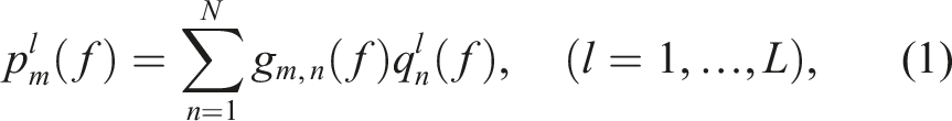
As illustrated in Figure 1, the process of sound pressure acquisition by the array is depicted. Multiple sources emit sound pressure outward, and the source plane is segmented into N different source points, which form the scan plane. The array, positioned parallel to this scanning plane at a distance d, consists of M microphones. The sound pressure at the N source points, as captured by the mth microphone, is expressed as The propagation model of an acoustic source in a free field is described as follows. The acoustic source plane is divided into N smaller planes, which are referred to as scanning planes. An array consisting of M microphones is established at a distance d from the scanning plane, in order to measure the sound field.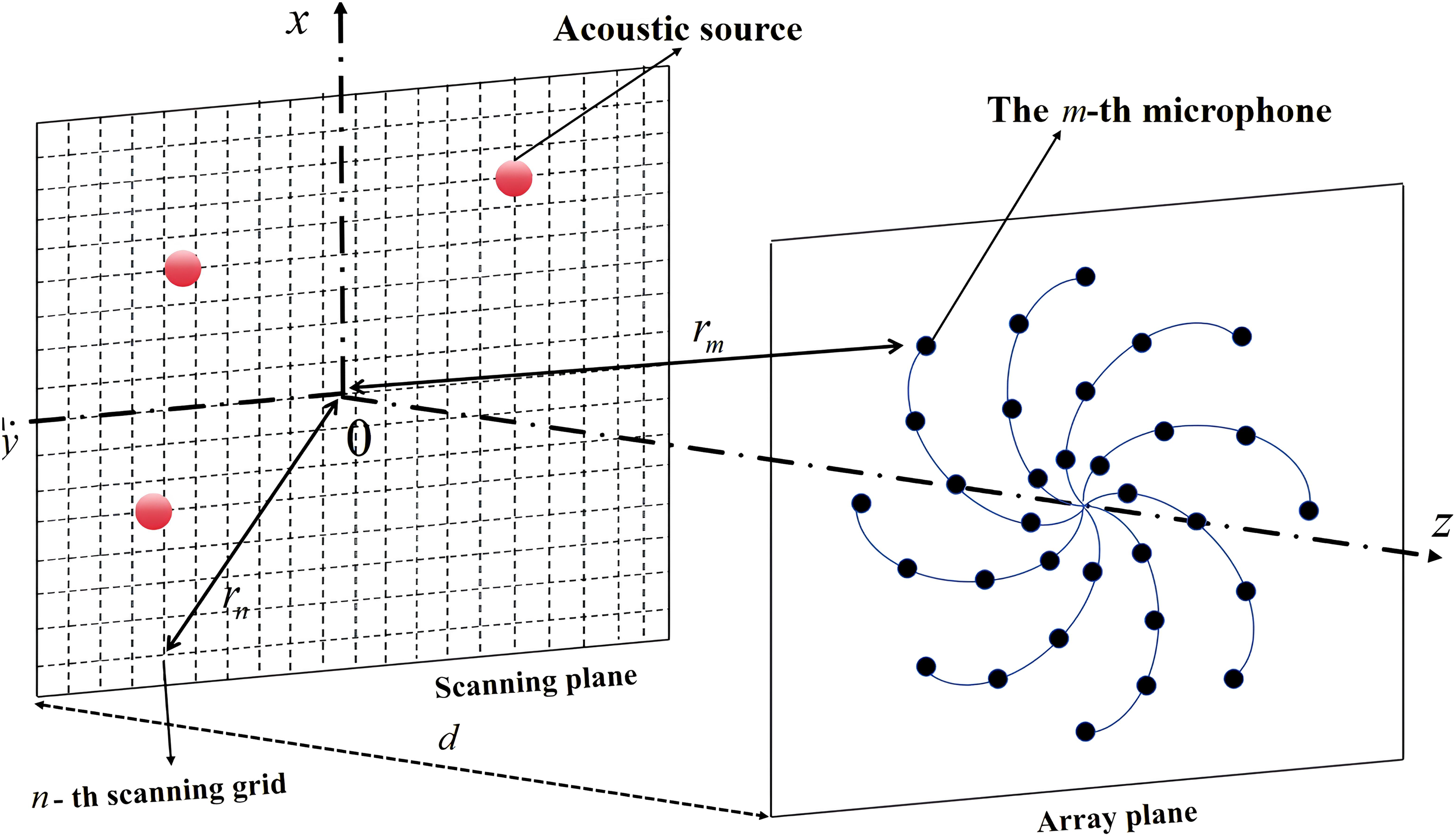
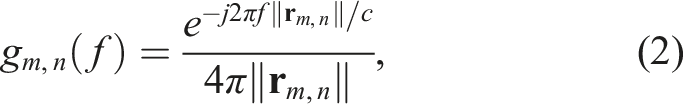
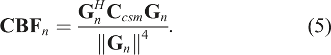
In free-field sound propagation, its transfer function can be considered as
The localization of the fault source is accomplished by assessing the magnitude of the energy at the location of the fault source, which constitutes an inverse acoustic problem. Beamforming exhibits superior capabilities for localizing the acoustic source and revealing its distribution.
2.2. Conventional beamforming method
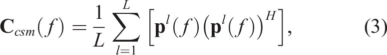
The principle of CBF employs the time (or phase in the frequency domain) difference of signals from each source point to each microphone to compute the direction vector. For the nth source point, the array synchronizes the signals from each microphone by adjusting their timing (or phase), ensuring temporal or phase alignment, and subsequently sums these signals to enhance focus on the nth source point, thereby obtaining the sound pressure at that location. This process is repeated for all N source points, yielding the sound pressure distribution across the scanning plane. Initially, the cross-spectral matrix of the array
Using various steering vectors, the original position of the acoustic source can be traced from the captured signal by the microphone array. The simplest of these steering vectors can be expressed as
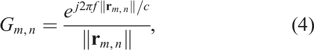
The beamforming output at the nth acoustic source point can be calculated as
CBF methods face difficulty in localizing the TAS among multiple rotating machine acoustic sources and background noise, but this challenge can be addressed by exploiting the inherent cyclostationary characteristics of rotating machine acoustic sources.
3. The cyclostationary of rotating mechanical signal
3.1. Description of first-order and second-order cyclostationary signals
If x(t) exhibits periodicity with period T, it is classified as a first-order cyclostationary signal. The cyclostationary characteristics of the first order cyclostationary signal

If the time-varying autocorrelation function

Finally, two stochastic signals x(t) and y(t) are considered jointly periodic with period T if their cross-correlation function

3.2. Cyclic spectral density
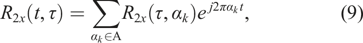
The cyclic autocorrelation function of a second-order cyclostationary signal is derived by applying Fourier series expansion to the time-varying autocorrelation function R2x (t, τ). This expansion is expressed as
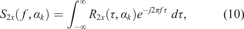
The CSD of a second-order cyclostationary signal is obtained by applying the Fourier transform with respect to the time-delay τ to the time-varying autocorrelation function R2x (τ, α). The expression is written as
3.3. Modeling of rotating mechanical signal
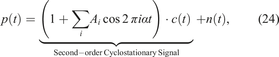
Rotating machinery signals primarily consist of first- and second-order cyclostationary signals overlaid with background noise and can be constructed as

4. Proposed acoustic source localization method
To overcome the limitation of the CBF method in extracting specific cyclostationary acoustic sources, the RRCR cyclic Wiener filter, which integrates the strengths of SUBLEX and MCR, is employed to extract SOIs at specific cycle frequencies. This filter is then utilized in conjunction with CBF for TAS localization in complex sound fields. The features of SUBLEX and MCR are as follows.
The SUBLEX method utilizes the cyclostationary characteristic of the signal to blindly extract the SOI through subspace decomposition. To achieve signal separation, the SUBLEX algorithm constructs a rank-1 projection matrix, denoted as 1. At least one cycle frequency is required by the SUBLEX method to extract the target acoustic source; 2. The SUBLEX method requires a number of microphones at least equal to the number of acoustic sources and is less effective at lower signal-to-noise ratios.
In contrast to the SUBLEX method, the MCR method exploits the spectral redundancy of the signal for denoising and reconstructs the SOI by frequency shifting the measured signal. The main aim of the MCR algorithm is to design a cyclic Wiener filter matrix, denoted 1. The MCR method can address both single-microphone and multi-microphone problems and is more effective at low SNR; 2. Multiple cycle frequencies are required by the MCR method to reduce the error in acoustic source extraction. The cyclic spectrum matrix of the MCR method does not possess the theoretical unit rank, resulting in some loss of statistical efficiency.
4.1. Beamforming based on reduced-rank cyclic regression (R-CBF) method
The prerequisite for the R-CBF method is the identification of at least one cycle frequency α, which is accomplished by employing CSD to determine α
k
of the array acquisition signal

The purpose of RRCR is to construct a suitable transfer matrix


The subspace projection matrix


By combining equations (14)–(16), the transfer matrix

Take equation (13) to obtain the extracted second-order cyclostationary signal
Suppose
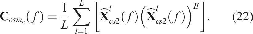
By bringing equation (22) and (4) into equation (5), the beamforming output of the nth acoustic source can be expressed as
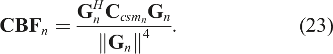
The TAS localization can be determined by repeating the beamforming operation for each acoustic source to obtain a complete acoustic map.
4.2. Acoustic source localization procedure using the R-CBF
The R-CBF method is summarized as follows: 1. First, a microphone array is utilized to collect the acoustic source signal; 2. The cyclic frequency of the SOI is estimated via CSD analysis of the time-domain signal collected by the array; 3. The frequency shift vector 4. By applying the cyclic Wiener filter 5. By incorporating the subspace projection matrix 6. Subsequently, CBF is utilized to achieve precise localization of the TAS.
5. Simulation analysis
5.1. Simulation setup
In the simulation, the composite sound field includes two inherently noisy cyclostationary sources with distinct periodic frequencies and one Gaussian white noise source. The signals from the cyclostationary sources are expressed as
In the simulation setup, a 36-channel multi-arm spiral array is configured. The sound field is discretized into a grid with a resolution of 0.01 m, spanning from −0.5 m to 0.5 m in both the Simulation overall layout, the plan uses a 36-channel multi-arm spiral array, with the acoustic source at a distance of 1 m from the array, and the three acoustic sources are located at coordinates source 1 at (0.3,0,0), source 2 at (−0.25,-0.25,0), noise at (0,0.3,0).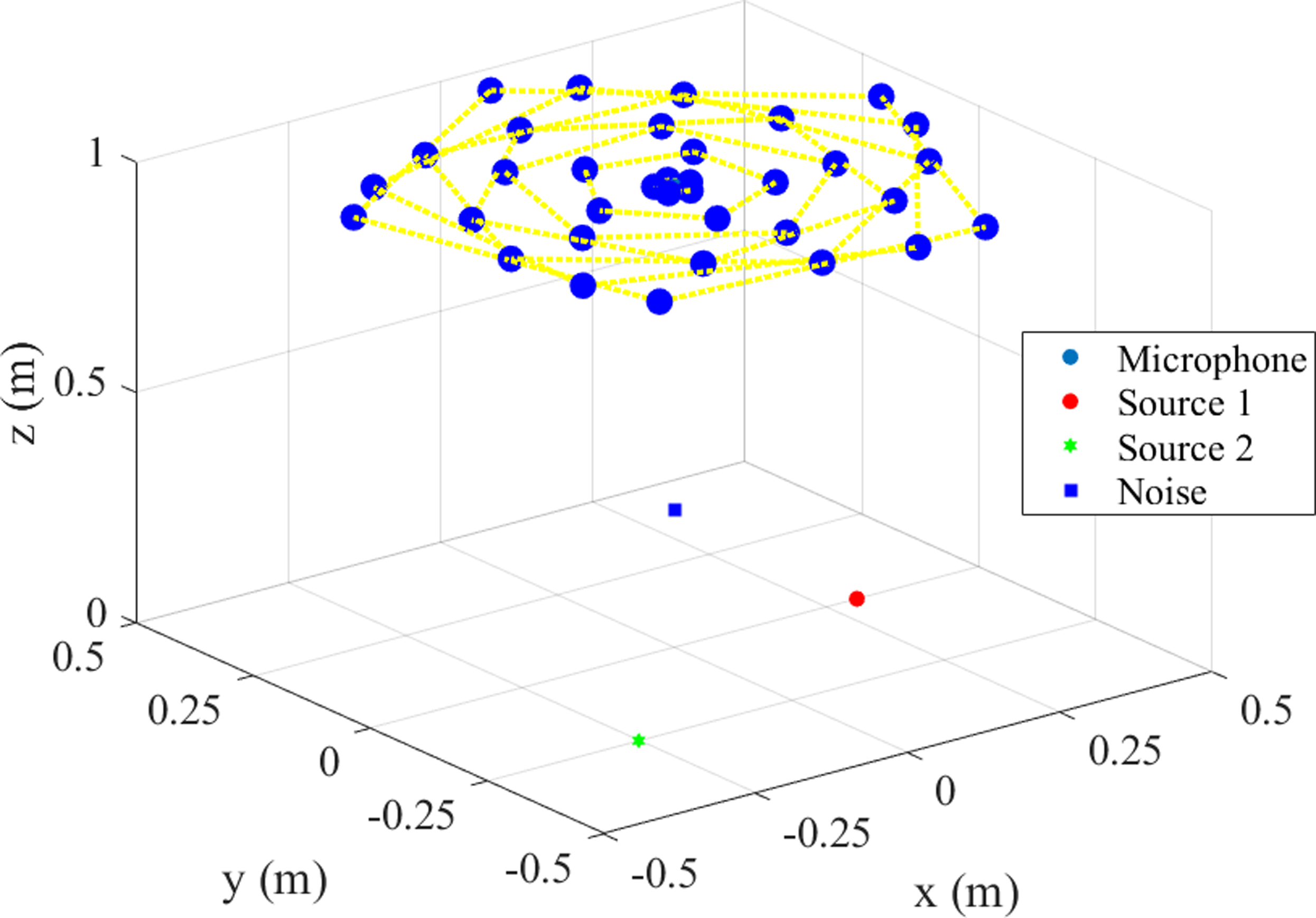
5.2. Simulation results
As illustrated in Figure 3, the PSD analysis of the single-channel signal from the microphone array, with a frequency range set from 0 to 4000 Hz, exhibits a uniform energy distribution across all frequencies, thereby obscuring the signal’s cyclostationarity. To address the issue of obscured cyclostationarity, a more thorough analysis was performed using the CSD method. The power spectral density of the single-microphone array signals does not exhibit a cyclostationary feature.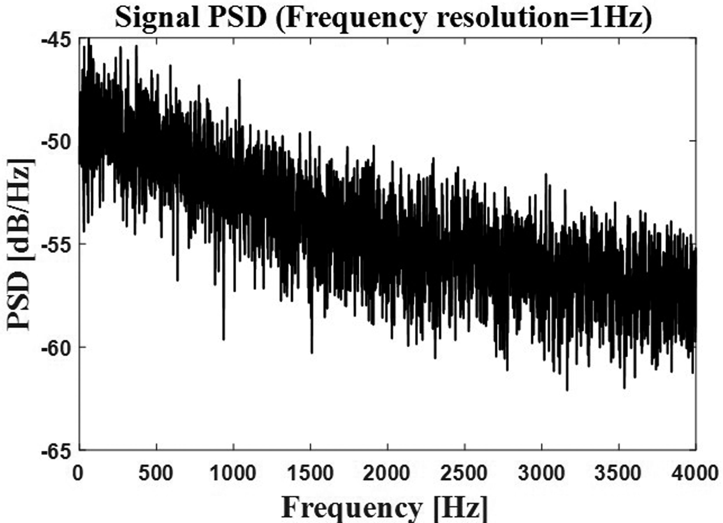
Figure 4(a) shows the mixed signals received by the array from three acoustic sources. It also shows simulated signals at cyclic frequencies of f
r
= 55 Hz and f
r
= 177 Hz, and their respective CSD analyses. The CSD results shown in Figure 4(a 4-6) reveal distinct peaks at f
r
= 55.0129 Hz and f
r
= 177.041 Hz, which are chosen as the target cyclic frequencies for RRCR filtering. The results of this filtering process are shown in Figure 4(b 1–4). The filtered signals exhibit cyclic frequencies of f
r
= 55.043 Hz and f
r
= 177.138 Hz, which closely approximate the simulated cyclic frequencies. The performance of the RRCR cyclic Wiener filter is verified. Figure (a) shows the three simulation signals set up and the corresponding CSD analysis. The three simulation signals are: mixed signal of three acoustic sources, simulation signal of periodic frequency α = 55 Hz, simulation signal of periodic frequency α = 177 Hz and corresponding CSD analysis. It can be seen that there are obvious peaks at α = 55.0129 Hz and α = 177.041 Hz. Figure (b) shows the signal with periodic frequencies of α = 55.0129 Hz and α = 177.041 Hz after RRCR filtering. The corresponding CSD analysis reveals distinct peaks at α = 55.043 Hz and α = 177.138 Hz. It can be seen from CSD analysis that the period frequency of the filtered signal is basically consistent with the simulation setting.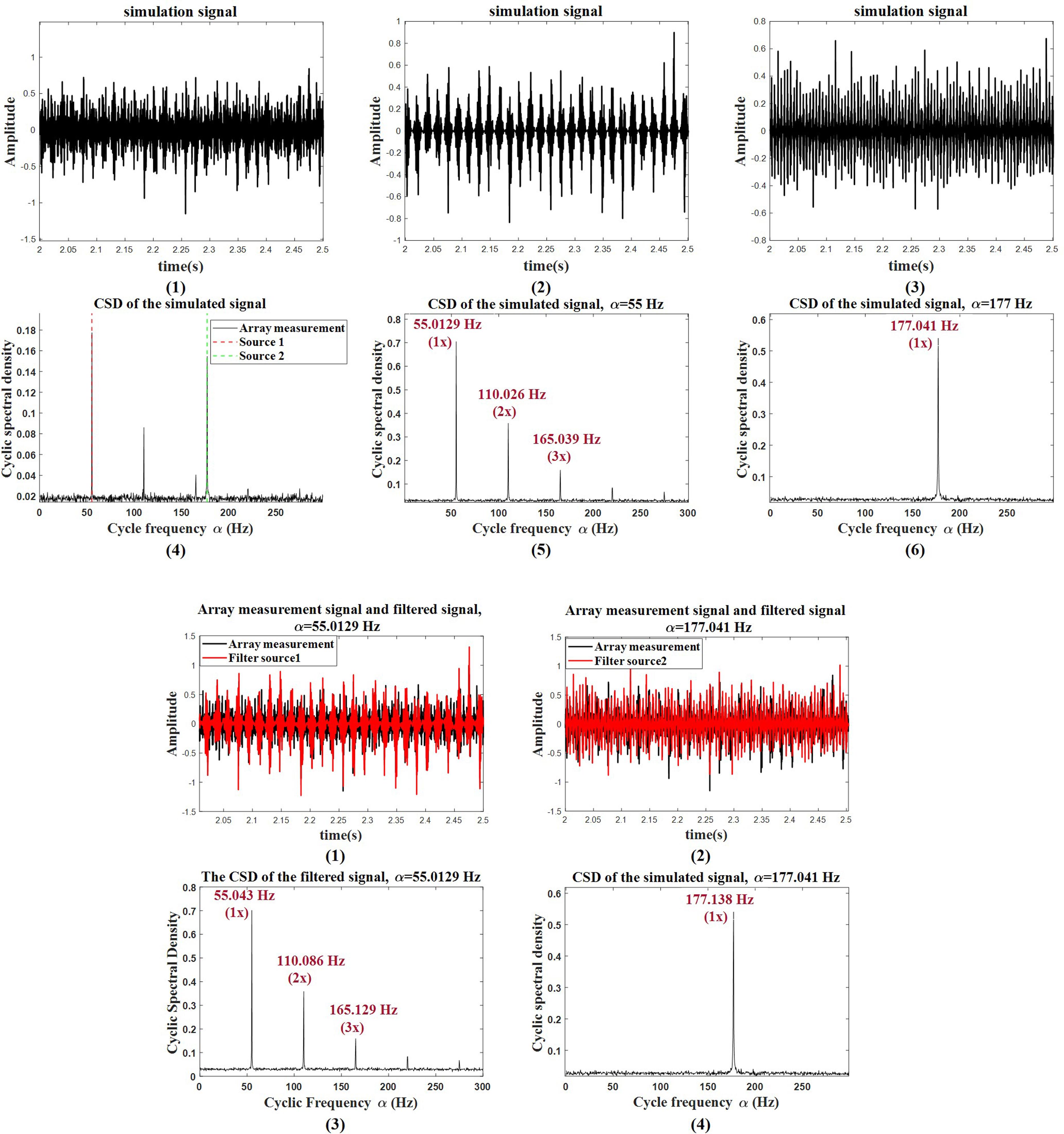
Figure 5 presents the results of the localization of the acoustic source obtained from CBF and R-CBF, where the cyan circles denote the actual position of the acoustic source. Figure 5(a) evaluates positioning in the frequency band from 1500 Hz to 8500 Hz. At 1500 Hz, the precise location of the noise source is not determined by CBF due to the broad main lobe. From 2500 to 8500 Hz, the CBF accurately identifies three sources; however, it is unable to extract acoustic sources at distinct cyclic frequencies. CBF, R-CBF, and Clean-SC-BF locates acoustic sources for α = 55 Hz and α = 177 Hz. Cyan circles represent the set acoustic sources localization.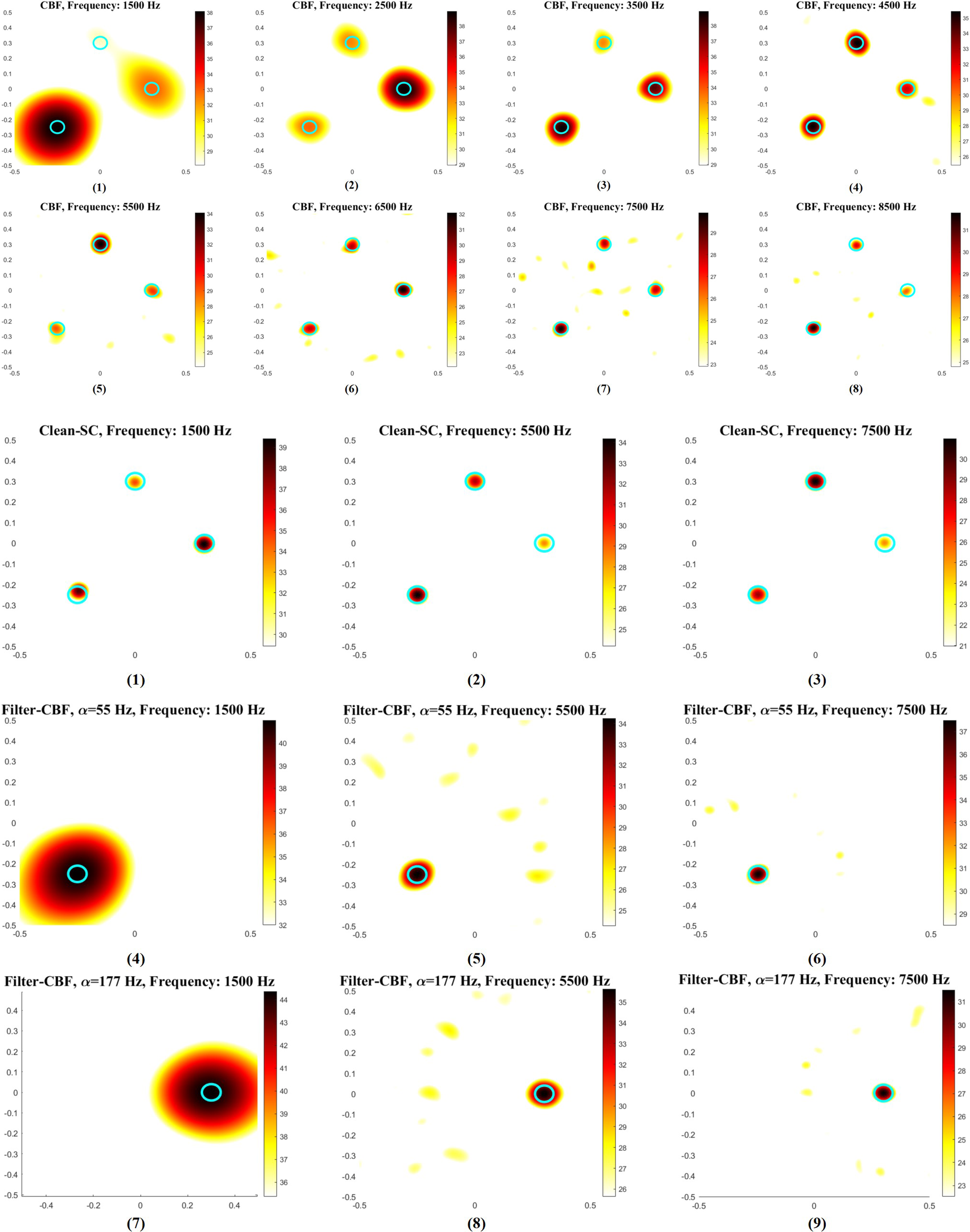
Figure 5(b) presents the localization results of the acoustic source obtained using the CLEAN-SC and R-CBF algorithms. Based on the performance of CBF at different frequency bands shown in Figure 5(a), evaluations were performed at 1500 Hz, 5500 Hz, and 7500 Hz. Clean-SC-BF has a narrower main lobe compared to CBF, allowing for clear differentiation of the three acoustic sources in the acoustic map. R-CBF effectively distinguishes sources at cyclic frequencies of α = 55 Hz and α = 177 Hz. Although its imaging at low frequencies is less resolution than that of Clean-SC-BF, R-CBF successfully isolates the target acoustic source from multiple sources and complex background noise, while maintaining low localization error. The localization error of R-CBF, quantified as the RMSE between the maximum sound pressure position in the acoustic image and the true source position, is lower than that of the other two methods, demonstrating the advantage of R-CBF, as shown in Figure 6(a-1). Source localization errors for three methods, R-CBF, CBF, and Clean-SC-BF, at different SNR, spectral frequencies f, distances d, cyclic frequency α from the source surface, and different array conditions, as well as source localization errors and computational costs for R-CBF at different numbers of microphones n.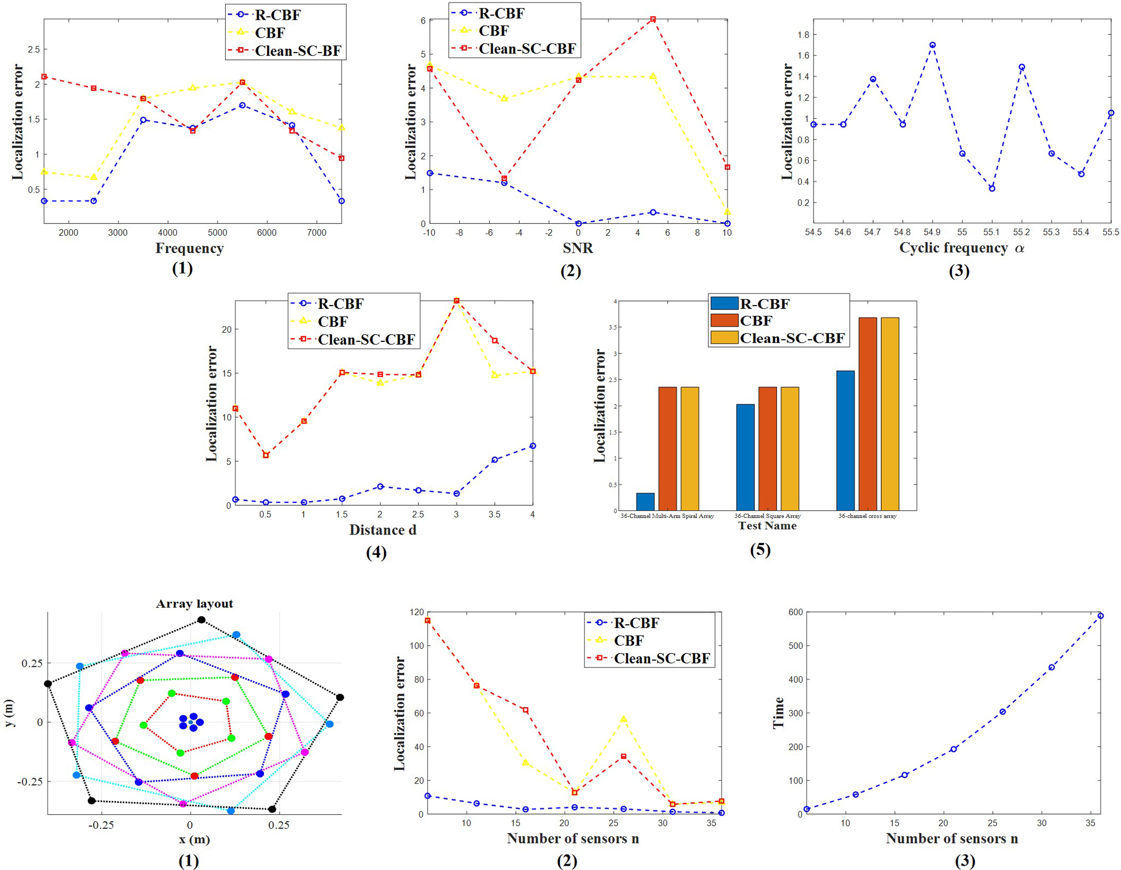
5.3. Evaluation of the effectiveness of the R-CBF method in multiple situations
Given that the accuracy of acoustic source localization can be affected by environmental factors and array configurations, various parameters have been established to evaluate the localization precision of R-CBF and compare it with that of CBF and Clean-SC-BF. The configuration of the acoustic source remains consistent with the simulation, wherein α = 55 Hz is designated as the target source, with the other two serving as interference sources. Furthermore, the spectral frequency for sound imaging is specified at 5500 Hz. The specific parameters established are as follows: 1. The SNR; 2. Cyclic frequency α. 3. The vertical distance between the array and acoustic source surface d; 4. Array type; 5. Number of microphones n.n
5.3.1. The SNR
To examine the influence of different SNR environments on the localization error of R-CBF, a 36-channel dobby spiral array was utilized, positioned 1 m away from the source surface, with an SNR range of [-10, 10]. The results depicted in Figure 6(a-2) reveal that R-CBF demonstrates notably better performance than CBF and Clean-SC-BF, sustaining a low localization error even at low SNRs. CBF and Clean-SC-BF, on the other hand, are prone to noise and interference from other acoustic sources, leading to compromised source localization accuracy. This validates the high accuracy of R-CBF in noisy environments.
5.3.2. Cyclic frequency α
In the experiment, a 36-channel dobby helical array was used, positioned 1 m from the source surface with an SNR of 0, to evaluate the effect of slight cyclic frequency variations on localization accuracy. By varying the cyclic frequency within the range [54.5, 55.5], Figure 6(a-3) shows that the localization error fluctuates within the range of 0–2, indicating that R-CBF is not significantly sensitive to these variations and maintains a very low error.
5.3.3. Distance between the array and the plane of the acoustic source d
In the experiment, a 36-channel dobby helical array was employed, positioned at varying distances from 0.1 to 4 m from the source surface with an SNR of 0, to examine the influence of array position on source localization error using the R-CBF method. Figure 6(a-4) reveals that CBF and Clean-SC-BF errors exhibited an increase with distance, whereas the error rate of R-CBF also showed an upward trend, remaining relatively low within the range of 0 to 4 m.
5.3.4. Array type
To investigate the impact of different array types on the acoustic source localization error of the R-CBF method, experiments were carried out using 36-channel spiral, square, and cross arrays, all positioned at a distance of 1 m from the source surface with an SNR of 0. The arrays were positioned 1 m from the source surface with an SNR of 0. The results, presented in Figure 6(a-5), show that spiral arrays outperform square and cross arrays in terms of acoustic localization, exhibiting lower errors. Furthermore, the R-CBF method proves superior to CBF and Clean-SC-BF under various array conditions.
5.3.5. Number of microphones n
To examine the impact of the number of microphones on source localization error, experiments were conducted using a spiral array configuration depicted in Figure 6(b-1), where the outer ring was augmented with five microphones at each experiment. The microphone count ranged from 6 to 36. The results, presented in Figure 6(b-2), indicate localization errors for R-CBF, CBF, and Clean-SC-BF decrease as the number of microphones increases, with R-CBF demonstrating the lowest error. However, Figure 6(b-3) reveals an increase in computation time with the addition of microphones. Therefore, an optimal balance between microphone count and signal length should be determined to control computational cost in practical applications.
Figure 6 shows that R-CBF achieved better results in the comparison of the three methods with different parameters and array configurations.
6. Acoustic source localization
6.1. Experimental setup
The feasibility of the R-CBF method in a real environment was verified through loudspeaker experiments. In the experiment, three acoustic sources were configured: two sources emitting cyclostationary sounds at α = 43.7 Hz and α = 147.3 Hz, and a third playing white Gaussian noise. The loudspeakers were positioned at coordinates (−0.35,-0.01,0) for Source 1, (0,-0.3,0) for the noise source, and (0.43,0,0) for Source 2. The array employed was a 36-channel multi-arm spiral array. Considering the far-field characteristics of beamforming, the source-to-array distance was set to 1 m. The sampling frequency was 25600 Hz with a recording duration of 10 seconds. Figure 7 illustrates the experimental setup. The acoustic experiment features two cyclostationary acoustic sources and one Gaussian white noise source. Source 1 is at (−0.36, −0.015, 0) with α = 43.7 Hz, Source 2 is at (0.4, 0, 0) with α = 147.3 Hz, and the noise source is at (0, −0.3, 0) .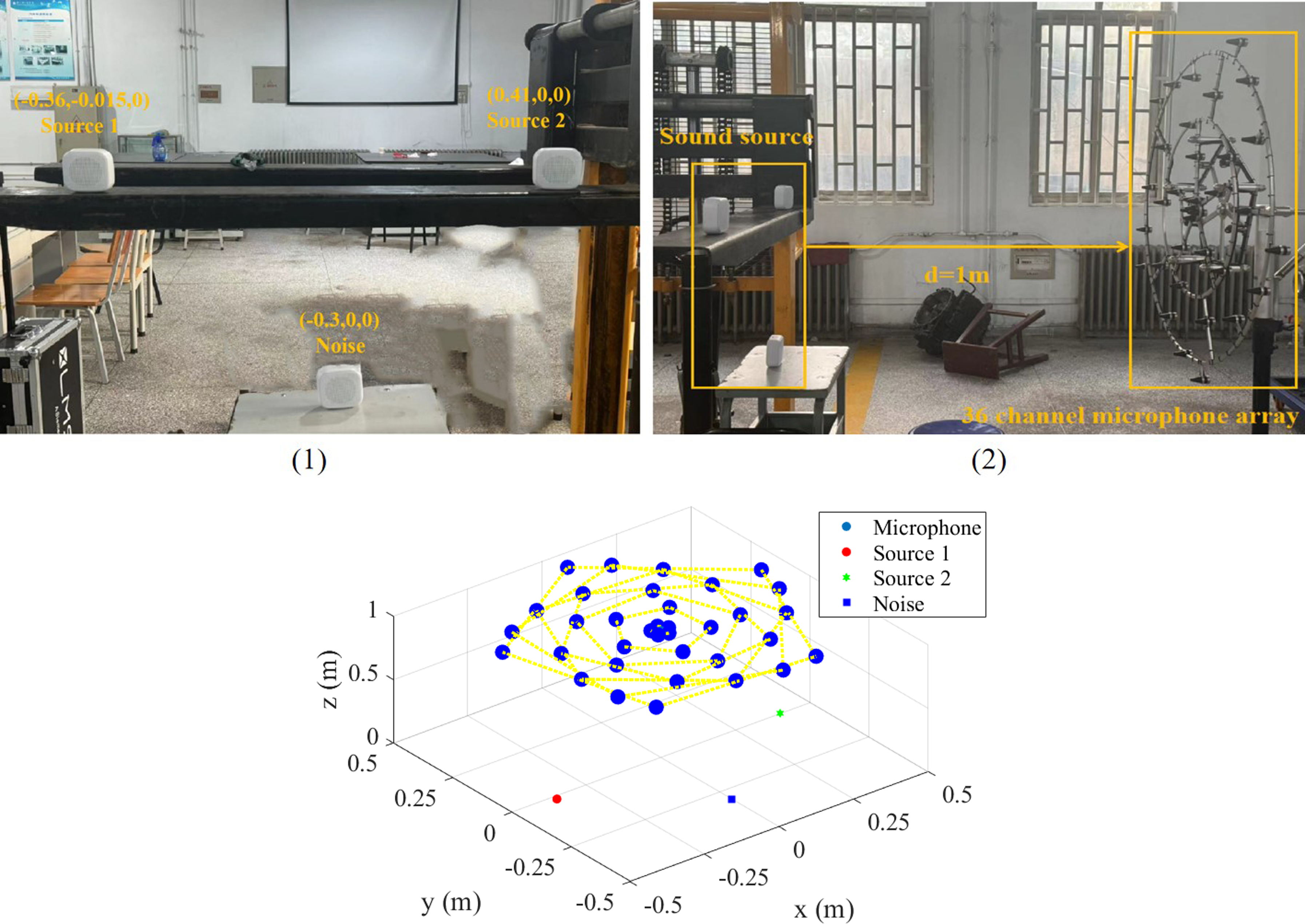
6.2. Experimental result
By analyzing the PSD and CSD of the array-captured signals, the alignment of the cycle frequencies of the actual signals with the experimental design can be ascertained. As illustrated in Figure 8, the PSD analysis exhibits an uneven distribution across the frequency spectrum, failing to reflect the cyclostationary nature of the signals. Figure 9 presents the array-measured signals, filtered signals, and the corresponding CSD analysis derived from the loudspeaker experiment. The CSD analysis of the array measurement signals in Figure 9(4) reveals wave peaks at α = 43.6082 Hz and α = 147.228 Hz, matching the preset cycle frequencies. Figure 9(2–3) presents the original and filtered signals with these cycle frequencies after applying the RRCR cyclic Wiener filter. The CSD analysis in Figure 9(3–4) reveals filtered signals with cyclic frequencies of α = 43.6082 Hz and α = 147.228 Hz, closely matching the simulated cyclic frequencies. The experimental results correspond to the preset cycle frequencies, confirming the RRCR’s ability for signal separation. The power spectral density of the single-microphone array signals does not exhibit a cyclostationary feature. The figure shows the array-acquired loudspeaker signals and the filtered signals extracted using the RRCR cyclic Wiener filter for cyclic frequencies of α=43.7 Hz and α=147.3 Hz and corresponding CSD analysis. (with the filtered signals shown in red and the array-acquired signals in black).It can be seen that there are obvious peaks at α = 43.6082 Hz and α = 147.228 Hz. 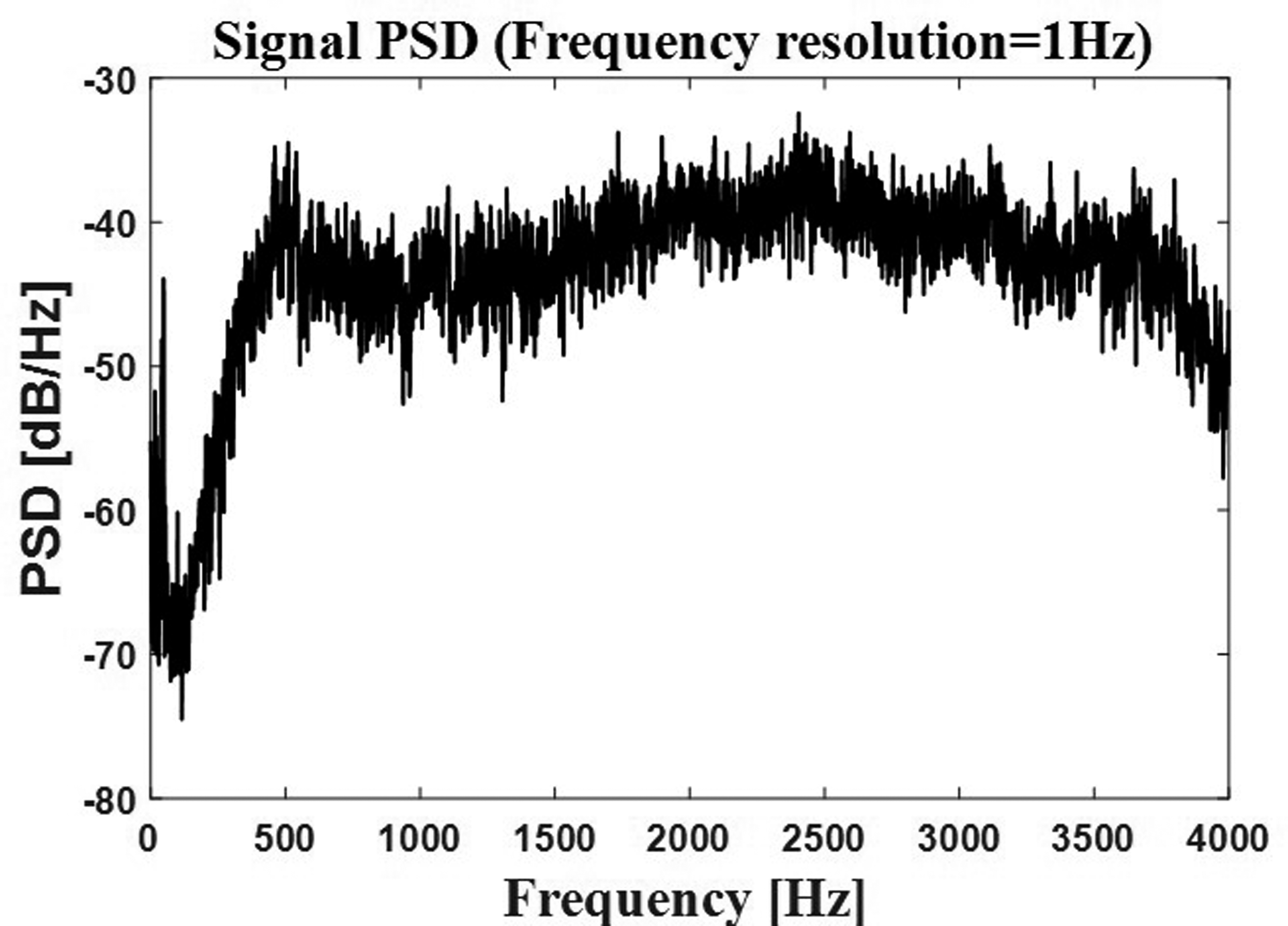
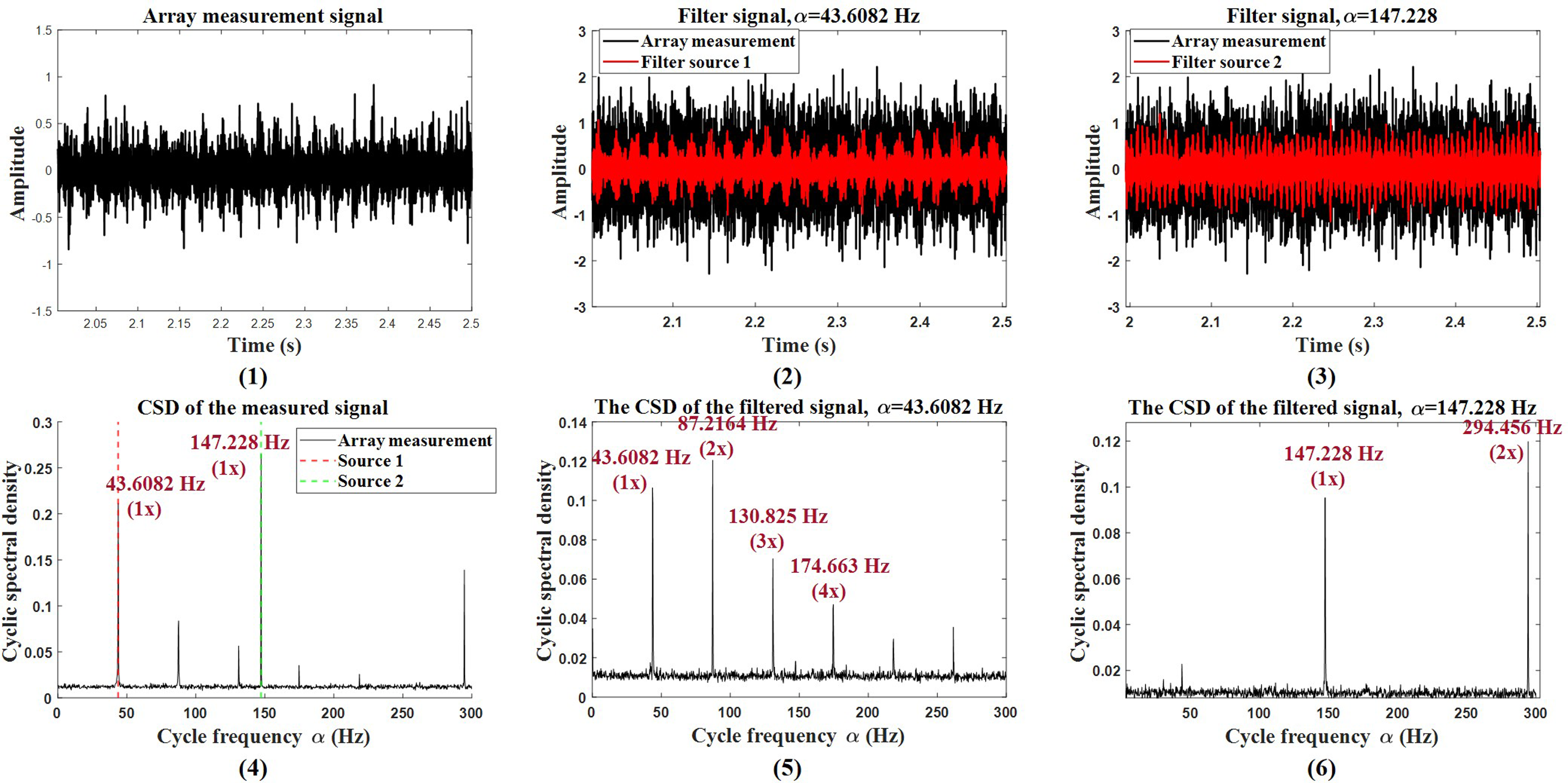
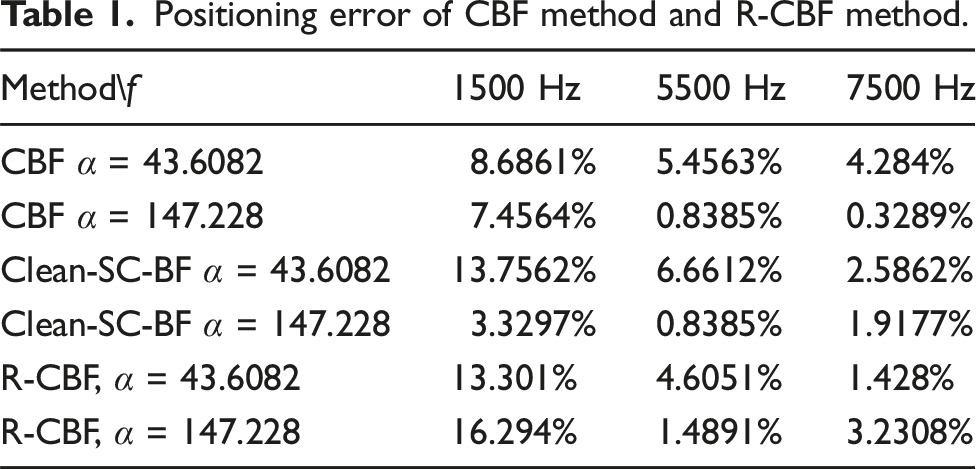
Figure 10(a) presents the localization results of the CBF method. At 1500 Hz, the main lobe is wider, resulting in lower spatial resolution. At 5500 Hz and 7500 Hz, side lobes appear, with more significant interference at 7500 Hz where the two cyclostationary sources are relatively weak compared to the noise sources due to noise interference; consequently, the cyclostationary sources are barely identifiable. R-CBF, Clean-SC-BF, and CBF locates acoustic sources for α = 43.6082 Hz and α = 177.449 Hz. Cyan circles represent the set acoustic sources localization.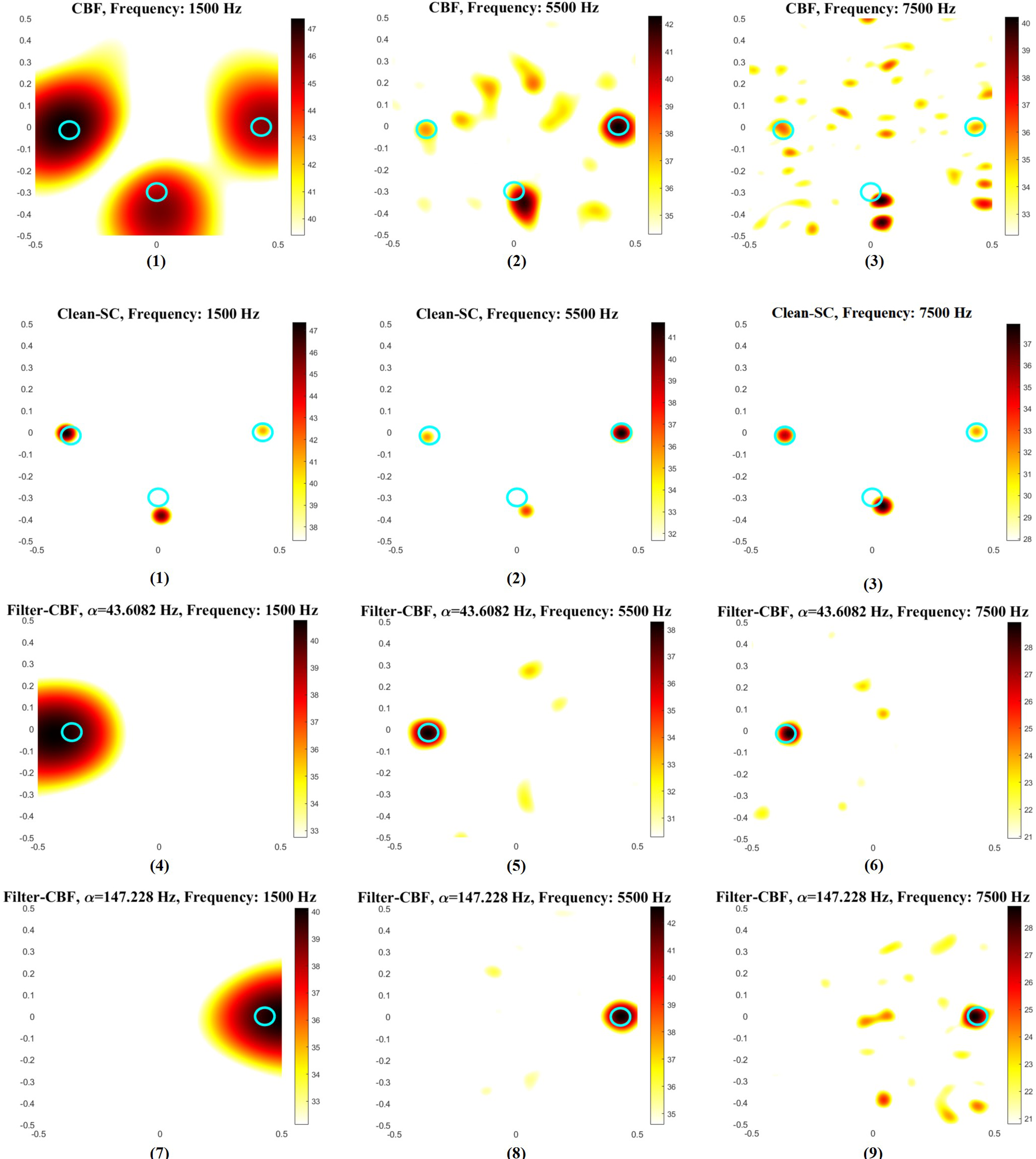
Positioning error of CBF method and R-CBF method.
Positioning error of CBF method and R-CBF method.
7. Bearing inner ring fault localization
7.1. Experimental setup
Experimental bearing parameters.
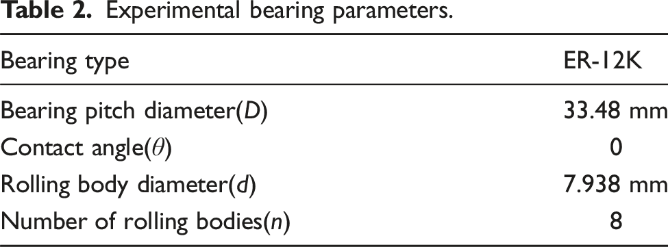
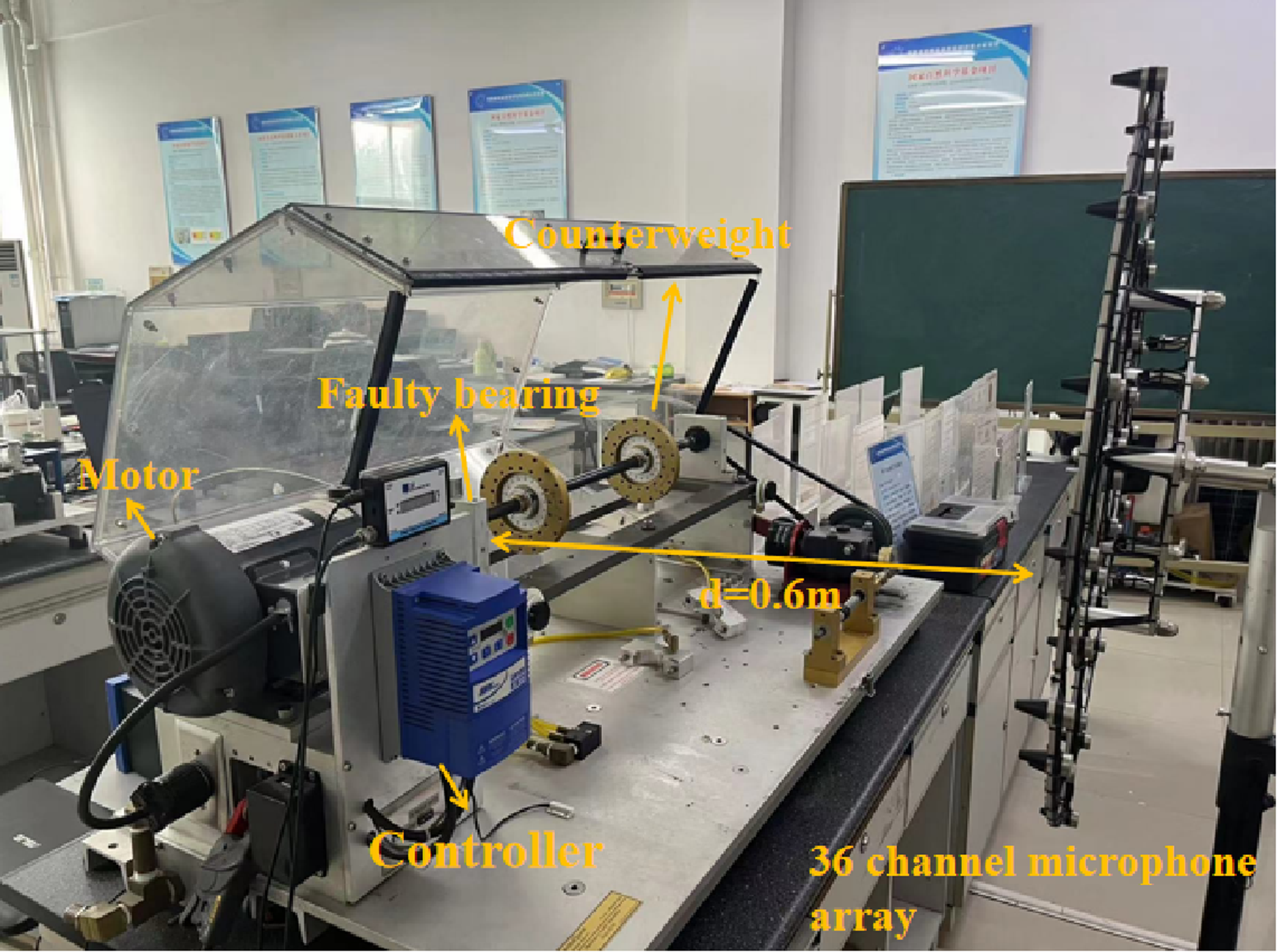
The failed bearing was an inner ring failure, mounted near the coupling end, with the bearing location specified as (−0.35, −0.23, 0). The 36-channel multi-arm spiral array is located at a distance of 0.6 m.
First, the signal acquired by the array is analyzed using CSD to ascertain its consistency with the theoretical prediction of the bearing’s inner ring failure frequency. The formula for calculating this failure frequency is given as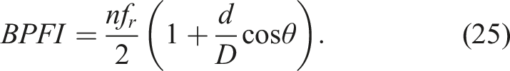
As shown in Figure 12(a), the signals captured by the arrays at bearing rotation frequencies fr of 20, 30, and 40 Hz are shown, along with their corresponding CSD analyses. The theoretical inner ring failure frequencies, calculated using equation (25) for fr of 20 Hz, 30 Hz, and 40 Hz, are 95.9677 Hz, 148.4516 Hz, and 197.935 Hz, respectively. However, the frequencies derived from the CSD analysis in Figure 12(a), 4-6) are 95.1328 Hz, 145.714 Hz, and 195.652 Hz, respectively, demonstrating very small errors from the theoretical values. Figure (a) shows the bearing signals with rotation frequency f
r
= 20 Hz, f
r
= 30 Hz, and f
r
= 40 Hz collected by the array, as well as the corresponding CSD analysis. The three true bearing failure frequencies are obtained as 95.1328 Hz, 145.714 Hz, and 195.652 Hz, respectively. Figure (b) extracted the filter signal SOI according to the fault frequency, and carried out CSD analysis on it. The fault frequency of the filter signal was obtained as 95.1328 Hz, 145.714 Hz, and 195.755 Hz, respectively.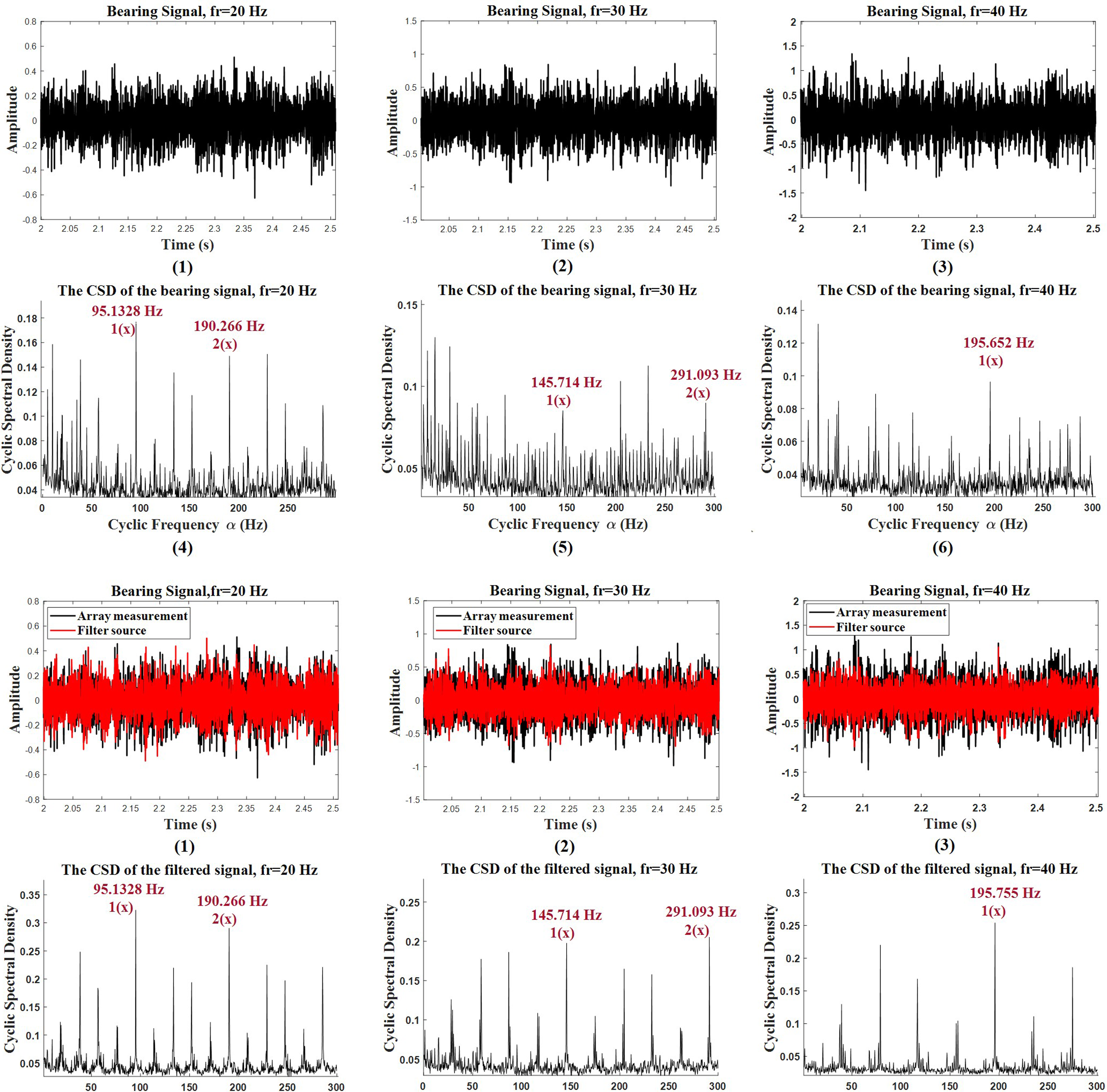
7.2. Experimental results
Based on the bearing signals collected by the array and CSD analysis presented in Figure 12(a), the RRCR cyclic Wiener filter was applied to isolate the signal of interest (SOI) corresponding to bearing failure frequencies of 95.1328 Hz, 145.714 Hz, and 195.652 Hz, as illustrated in Figure 12(b 1–3). The CSD analysis of the filtered signal, depicted in Figure 12(b 4–6), reveals fault characteristic frequencies of 95.1328 Hz, 145.714 Hz, and 195.755 Hz, with negligible deviation from the theoretical fault frequencies. Furthermore, the peak values in the CSD of the filtered signal are more pronounced compared to those CSD of the original array measurement signal.
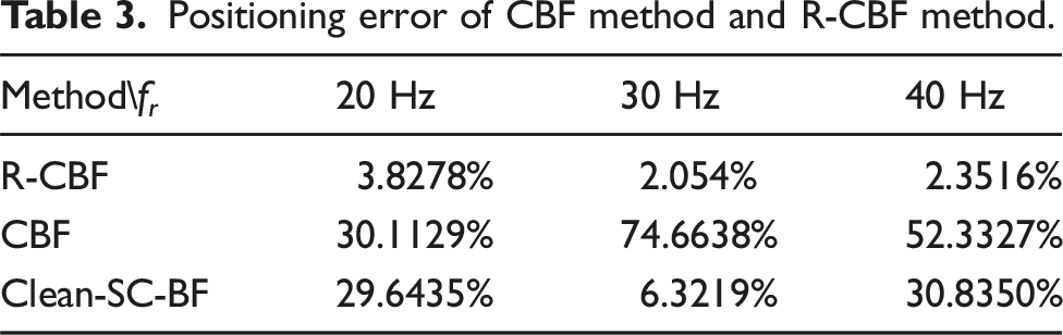
The center frequencies of the bearing signal’s resonance band, determined via kurtogram analysis as 3890.6 Hz, 3631.3 Hz, and 3804.2 Hz (rounded to 3890 Hz, 3632 Hz, and 3804 Hz), are utilized as imaging frequencies due to the high SNR in the experiment, as illustrated in Figure 13(a). Figure 13(b) shows the localization results obtained using the CBF, Clean-SC-BF, and R-CBF methods at speeds of 20, 30, and 40 Hz. The true position of the bearings is indicated by a cyan circle. Combined with the information in Tables 3, it is evident that the CBF method produces poor localization results, unable to locate the acoustic source of the faulty bearing, with localization errors reaching 30.1129%, 74.6638%, and 52.3327% at three different rotational frequencies. Similarly, the Clean-SC-BF method deviates from the true position, with localization errors of 29.6435%, 6.3219%, and 30.8350% at these frequencies. In contrast, the R-CBF method distinctly identifies the fault acoustic source at the faulty bearing’s position, with lower localization errors of 3.8278%, 2.054%, and 2.3516% at the same rotational frequencies, despite the presence of some side lobes, but affirming the method’s potential in fault diagnosis. Figure (a) represents the kurtosis diagram of the rotation frequency f
r
= 20 Hz, f
r
= 30 Hz, and f
r
= 40 Hz; Figure (b) represents the acoustic source location diagram of CBF, Clean-SC-BF, and R-CBF. Cyan circles represent the set acoustic sources localization.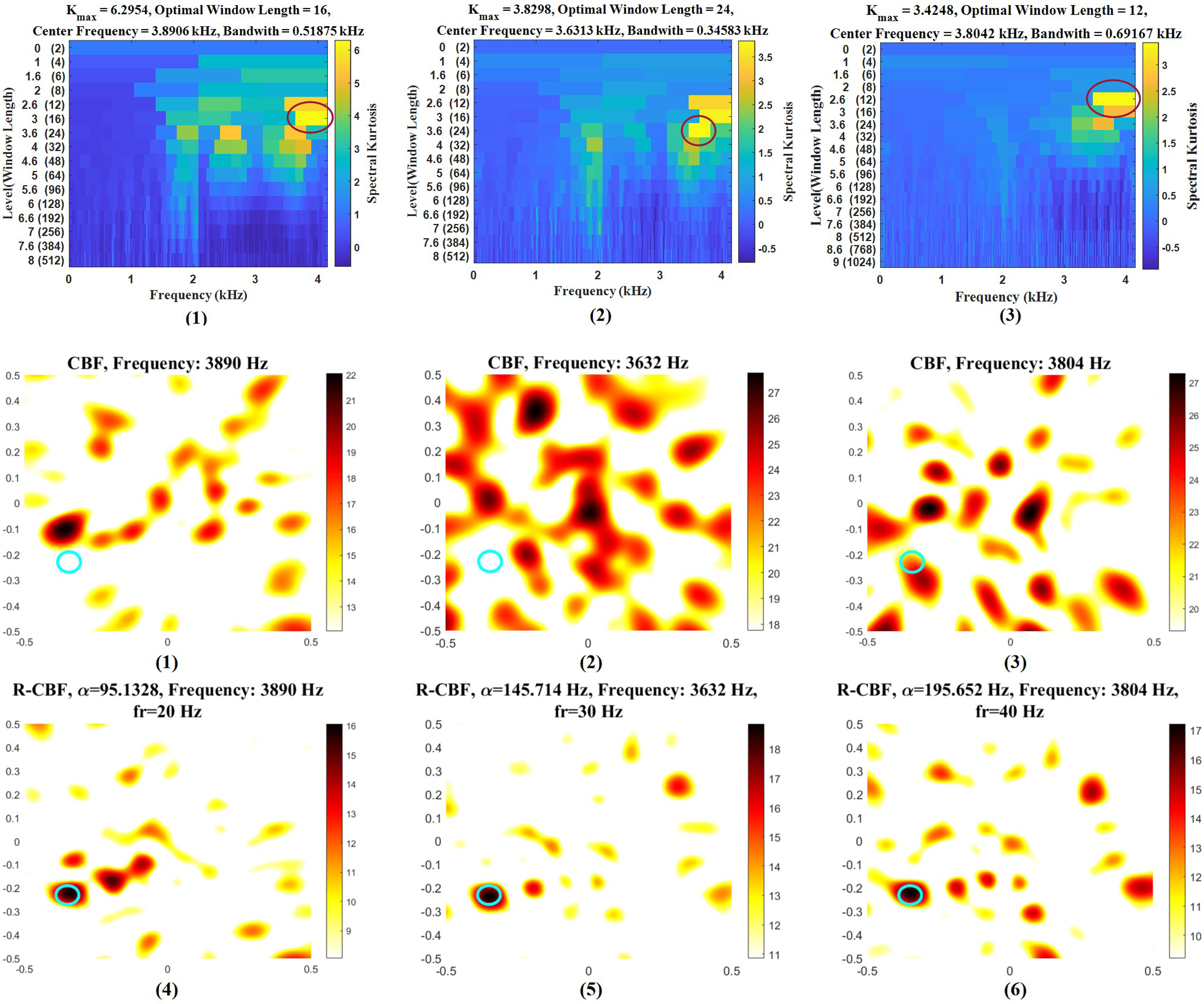
8. Conclusions
In this paper, a method called R-CBF is proposed to localize the sound sources associated with rotating mechanical faults. Using the cyclic frequency as an a priori condition, the measured signal is frequency shifted to derive its frequency shifted matrix. Subspace decomposition is subsequently applied to this matrix to construct the RRCR Cyclic Wiener filter, enabling the separation of the SOI. By integrating this filter with the CBF method, the faulty acoustic source is successfully separated. The R-CBF method is validated through simulations and loudspeaker experiments, and bearing experiments are performed to evaluate its performance in real-world environments, confirming its potential for fault diagnosis. The detailed conclusions regarding the proposed R-CBF methodology are presented below. 1. The integration of beamforming with the RRCR cyclic Wiener filter overcomes the limitations of CBF and sources with different cyclic frequencies and reduces noise interference in low SNR conditions; 2. In practical applications targeting rotating machinery faults, the methodology successfully addresses the challenges posed by noise and various interfering acoustic sources, resulting in the accurate localization of the fault acoustic source and confirming its potential effectiveness in the field of fault diagnosis; 3. The R-CBF method exhibits shortcomings, including an increased microphone count that leads to significantly higher time costs compared to the CBF and Clean-SC-BF methods, as well as poor spatial resolution for acoustic source localization at low frequencies. In practical applications, the high computational time poses a significant drawback that impedes implementation. Future research will focus on simplifying the computational process, significantly reducing the time cost, and improving the spatial resolution of acoustic source imaging to address these issues.
Footnotes
Declaration of conflicting interests
The author(s) declared no potential conflicts of interest with respect to the research, authorship, and/or publication of this article.
Funding
The author(s) disclosed receipt of the following financial support for the research, authorship, and/or publication of this article: This work was supported by National Natural Science Foundation of China (Grant No. 12474464) and National Natural Science Foundation of China (grant number: 12302270), partly supported by the Key Scientific and Technological Project of Henan Province (grant numbers: 242102221003 and 232300420090), and partly supported by the Key Research and Development Projects in Henan Province in 2022 (grant number: 221111240200).