Sage Journals: Discover world-class research

Abstract

The dynamic properties of joints, or inter-component connections, are a principal source of uncertainty when modelling complex built-up structures. In the present paper, we propose an interval-based sensitivity analysis (SA) to establish the contribution, or influence, of a structure’s uncertain joint dynamics towards the uncertainty of its coupled admittance. We choose an interval SA as it overcomes the limitations of conventional local and global methods; accuracy and computation efficiency, respectively. Furthermore, it avoids the need for detailed probabilistic data to describe each joint, which is often unavailable. The proposed interval SA is based on the dual formulation of the sub-structuring problem and utilises the Sherman–Morrison formula to factor out the contribution of an individual joint. A complex interval is used to represent the uncertain joint stiffness and damping, and precise bounds on the assembly’s complex admittance (also operational response) are determined following an application specific algorithm. The relative change between input (joint stiffness and damping) and output (complex admittance) interval area is chosen as a sensitivity metric and used to rank order the uncertain influence of each joint. The method is illustrated by numerical example.

Keywords

interval sensitivity analysis joint dynamics uncertainty propagation possibilistic

1. Introduction

Complex engineering structures (such as vehicles, satellites, domestic products, buildings and more) are built-up from individual components that are joined with connections that rely on frictional contact or other dissipative mechanisms (such as elastomeric elements). These inter-component connections, or joints, are a principal source of uncertainty when modelling such structures.

The types of joints encountered in practical engineering structures are wide ranging, and can include bolted connections, rivets, welds and resilient elements, among many others (Ibrahim and Pettit, 2005). Likewise, their dynamics can vary greatly, from linear spring or beam-like coupling, to non-linear hysteretic, perhaps discontinuous (e.g. frictional), connections (Segalman, 2006; Marques et al., 2016). To accurately model the dynamics of a jointed structure, it is necessary to characterise the dynamics of its constituent joints; experimentally, this is a demanding task (Ren and Beards, 1995, 1998; Čelič and Boltežar, 2008; Noll et al., 2013; Tol and Özgüven, 2015; Roettgen and Allen, 2017; De Oliveira Teloli et al., 2021), often requiring supplementary numerical models (Saeed et al., 2020b,a), and is subject to considerable experimental uncertainty.

In the development or refinement of a numerical model it is important to establish the contribution of each uncertain parameter towards the uncertainty of the model output. This is the role of Sensitivity Analysis (SA) (Saltelli et al., 2008). Methods of SA can be broadly categorised as local or global. Local methods consider linearisation of the model and are appropriate only when low level uncertainty, or weak non-linearity, is present. Based on sampling strategies, global methods consider the entire range of model behaviour and take into account non-linear effects due to large parameter variation.

When dealing with problems of uncertainty, there are two further classifications, or viewpoints: probabilistic or non-probabilistic. Conventional SA is probabilistic, describing uncertain parameters by their probability distributions. One of the principal difficulties in evaluating the uncertainty of a complex system by probabilistic means is the acquirement of detailed statistical input data. In the absence of such data, complex statistical analysis cannot be justified. It is this issue that lead to the development of non-probabilistic, or ‘possibilistic’, analysis methods, which include interval analysis (Rao and Berke, 1997; Moens and Vandepitte, 2004; Muscolino et al., 2014; Łasecka-Plura and Lewandowski, 2017; Lei et al., 2019; Imholz et al., 2020; Zhao et al., 2021), convex modelling (Ben-Haim and Elishakoff, 2013) and fuzzy set theory (Chen and Rao, 1997; Yin et al., 2016). As the name suggests, possibilistic methods are not concerned with establishing the probability of an outcome occurring, rather whether or not is it possible, regardless of its likelihood.

Given the experimentally demanding nature of joint characterisation, it is often challenging to obtain the necessary statistical information to conduct a probabilistic analysis of uncertainty. For this reason, possibilistic analysis methods offer a convenient alternative. In the present paper, we consider, in particular, an interval-based analysis of joint dynamics, where uncertain joint parameters (stiffness and damping) are treated as unknown but bound by upper and lower limits.

Interval-based methods have found numerous applications in the analysis of structural dynamic systems, including interval Finite Element Analysis (Moens and Vandepitte, 2004; Muscolino et al., 2014), eigenfrequency analysis (Chen et al., 2003, 2009), robustness evaluation (Fujita and Takewaki, 2011), quantification of experimental uncertainty (Zhao et al., 2021), inverse force identification (Lei et al., 2019), stochastic response analysis (Muscolino and Sofi, 2012, 2013), among many others. Of particular relevance to the present paper is its application to SA.

In 2007, Moens and Vandepitte introduced the concept of interval sensitivity theory for analysing systems subject to interval-based uncertainty. In contrast to conventional local SA, interval SA is not limited to the first order behaviour of the system understudy. Rather, it considers the entire range of dynamics permissible within the parameter’s interval bounds. In brief, their proposed interval SA considered the relative change in absolute interval widths on the input and the output side of the problem. Utilising a mixed optimisation and interval arithmetic strategy, a numerical example was presented whereby the frequency response function of a lumped parameter truck model was subject to an interval SA with respect to its lumped mass values.

In the present paper, we propose a (conceptually) similar interval SA methodology to identify (and rank order) the uncertainty contribution of individual joints within a complex built-up structure.

The proposed analysis is based on the dual formulation of the sub-structuring problem and utilises the Sherman–Morrison formula to factor out the contribution of an individual joint. The considered joint dynamics are limited to those of linear spring-damper like connections. Though simple in form, joints of this type have been used successfully to improve estimates of coupled assembly dynamics (Saeed et al., 2020b,a). The stiffness and damping of each joint is represented by a complex rectangular interval, and is used to establish precise interval bounds on the coupled assembly’s complex admittance (also its operational response). To rank order the influence of each joint, we consider the relative change between the input (joint stiffness and damping) and output (complex admittance) interval area as a sensitivity metric. These developments are illustrated by a numerical example.

Having introduced the context of this paper, its remainder is organised as follows. Section 2 begins by introducing the governing component-based equations for complex structures with flexible interface dynamics. Section 3 provides some detail on interval analysis, including complex interval representations, and describes the concept of interval SA. Section 4 considers the interval assessment of joint variability, before section 5 demonstrates the proposed joint interval SA by numerical example. Finally, section 6 draws some concluding remarks.

2. Dual representation of flexible interface dynamics in complex built-up structures

When analysing the properties of complex structures, and the influence of joint dynamics, it is convenient to adopt a component-based approach where each structural component (s) is represented by its free interface admittance matrix Y_(s). This can be obtained numerically by inversion of the dynamic stiffness matrix Z_(s)

Y_{(s)} = Z_{(s)}^{- 1}, Z_{(s)} (ω) = K_{(s)} + i ω C_{(s)} - ω^{2} M_{(s)},

(1)

where M, K and C represent the discretised mass, stiffness and damping matrices of the component (Petyt, 2010), or equivalently, assuming proportional or structural damping, by modal summation

Y_{(s)} = Φ_{(s)} {[Λ_{(s)} - ω^{2} I + i ω {\bar{C}}_{(s)}]}^{- 1} Φ_{(s)}^{T},

(2)

where Φ is a truncated matrix of mass normalised mode shapes, Λ is a diagonal matrix containing the squared natural frequencies,

\bar{C}

is a modal damping matrix that describes the component’s damping characteristics (its form will depend on the type of damping considered), and I is an identity matrix (Ewins, 1984). Alternatively, Y_(s) can be determined experimentally using standard measurement techniques (International Organization for Standardization, 1994).

The components that comprise built-up structures may be classed as either active, or passive. Active components contain vibration generating mechanisms, and include motors, engines, pumps, etc. Passive components simply transmit or radiate energy. A generic two component active-passive assembly is depicted in Figure 1. Each component is represented by two sets of DoFs, the interface set c and the internal set a or b. This picture may be readily generalised to an arbitrary number of components.

Figure 1.

General active-passive assembly (AB) with joint (J) flexibility. The relative interface displacement at the nth connection δ_n = u_An − u_Bn is proportional to the interface flexibility γ_n and the internal coupling force λ_n. a and b represent internal DoFs, c are the interface DoFs, and o is the internal region where operational forces develop.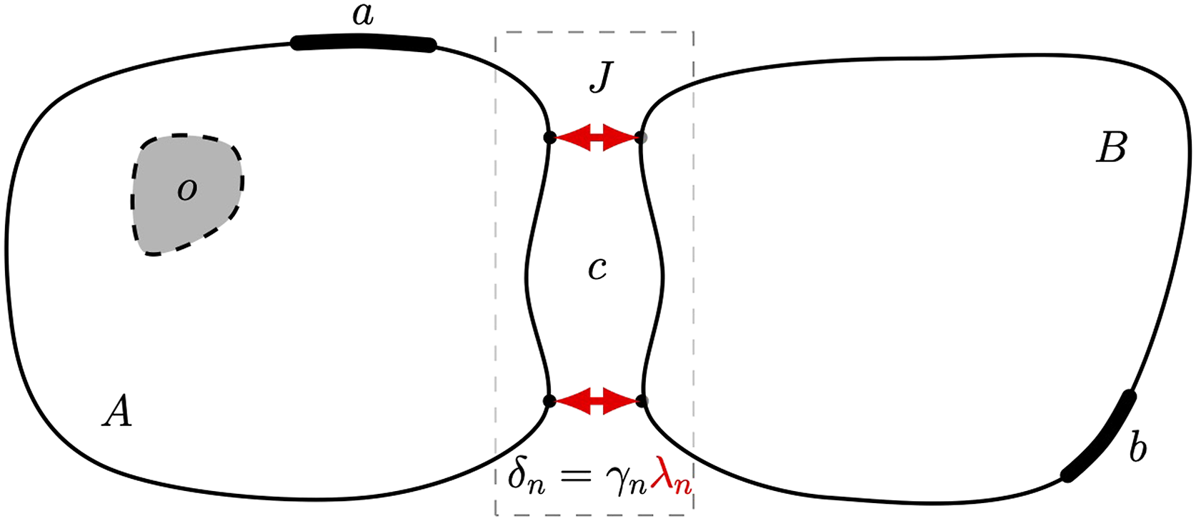

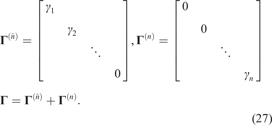
The equations of motion representing an uncoupled system of S components are given by

Z u = f + g,

(3)

where Z is a block diagonal dynamic stiffness matrix, and u, f and g are stacked response, external force and interface force vectors, respectively. To rigidly assemble the components, the conditions of continuity and equilibrium must be satisfied. These are expressed concisely in matrix form, respectively, by

B u = 0

(4)

and

L^{T} g = 0,

(5)

where B and L represent signed and unsigned Boolean matrices (De Klerk et al., 2008).

In the presence of a flexible interface, for example, due to a spring-damper joint, continuity is not satisfied. Rather

B u = δ = Γ λ,

(6)

where the interface separation δ is related to the unknown joint force λ by an interface flexibility matrix Γ. For the spring-damper joint considered here, this flexibility matrix is given by

\begin{array}{l} Γ & = [\begin{matrix} {(\frac{1}{k + i r})}_{1} \\ ⋱ \\ {(\frac{1}{k + i r})}_{N} \end{matrix}] \\ = [\begin{matrix} {(γ_{r} + i γ_{i})}_{1} \\ ⋱ \\ {(γ_{r} + i γ_{i})}_{N} \end{matrix}] \end{array}

(7)

γ_{r} = \frac{k}{{| Z |}^{2}}, γ_{i} = - \frac{r}{{| Z |}^{2}}, Z = k + i r,

(8)

where N denotes the number of connections, and k and r are the joint stiffness and damping.

To satisfy equilibrium, the interface force g is given the form

g = - B^{T} λ,

(9)

where λ are the unknown joint forces and B is a signed Boolean matrix. The presence of B^T ensures that the forces applied to neighbouring components are equal and opposite, thus satisfying equilibrium.

The unknown joint forces λ are found using the relaxed continuity condition as follows. The interface force g is substituted into the EoM

u=Y (f+g),

(10)

where Y is the uncoupled admittance matrix, to give

u = Y (f - B^{T} λ),

(11)

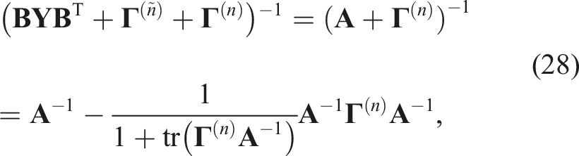
Equation (11) is substituted into the relaxed continuity condition (equation (6))

B Y (f - B^{T} λ) = Γ λ,

(12)

Solving for λ then yields

λ = {(B Y B^{T} + Γ)}^{- 1} B Y f .

(13)

Finally, substituting equation (13) into equation (11) leads to,

Y_{C} = Y - Y B^{T} {(B Y B^{T} + Γ)}^{- 1} B Y,

(14)

which is an equation for the coupled admittance of the assembly. Note that in the presence of a rigid connection, γ_n → 0.

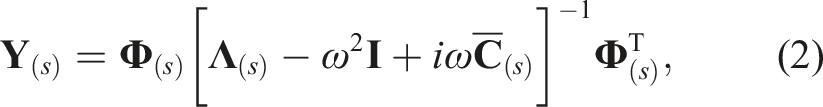
In the present paper we are interested in the sensitivity/uncertainty of the coupled admittance Y_C due to the unknown, but bounded, interface flexibility γ_n.

3. Interval analysis

Interval analysis falls within a family of non-probabilistic methods for evaluating uncertainty in complex systems (Langley, 2000; Faes and Moens, 2020). One of the main difficulties when evaluating the uncertainty of a complex system by probabilistic means is the acquirement of detailed statistical input data. This is particularly so for joint dynamics. In the absence of such data, complex statistical analysis cannot be justified. It is this issue that has lead to the development of non-probabilistic, or ‘possibilistic’, analysis methods.

With an interval-based analysis, the uncertain parameter x is not treated statistically. Rather, it is taken to be bounded, such that

\underline{x} < x < \bar{x},

(15)

where

\underline{□}

and

\bar{□}

denote lower and upper bounds, respectively. As an interval, {x} is characterised by a pair of numbers representing its lower and upper bounds

{x} = [\underline{x} \bar{x}] = [x_{c} - x_{Δ} x_{c} + x_{Δ}],

(16)

where we define the interval mid-point and half width, respectively, as

x_{c} = \frac{\underline{x} + \bar{x}}{2} and x_{Δ} = \frac{\bar{x} - \underline{x}}{2} .

(17)

Unlike a probability distribution, the interval bounds provide no detailed information on the likelihood of a particular value of x, only that its true value must occur within the stated bounds.

There are two common ways to extend the interval representation to complex variables (required to represent joint stiffness and damping). In one, the complex interval is represented by a circular disk in the complex plane, characterised by its centre point and radius (Petkovic and Ljiljana, 1998; Rump, 1999). In the other, the real and imaginary parts of the complex number are represented by independent real intervals. This leads to a rectangular interval in the complex plane (Petkovic and Ljiljana, 1998; Rokne and Lancaster, 1971; Lohner and Gudenberg, 1985). In the present paper, we will adopt the rectangular complex interval representation as it enables the independent assignment of joint stiffness and damping.

Adopting the centre point and half width notation above, a complex rectangular interval takes the form

\begin{array}{l} {z} & = {x} + i {y} \\ = [x_{c} - x_{Δ} x_{c} + x_{Δ}] + i [y_{c} - y_{Δ} y_{c} + y_{Δ}], \end{array}

(18)

an example of which is shown in Figure 2.

Figure 2.

Example of a complex rectangular interval.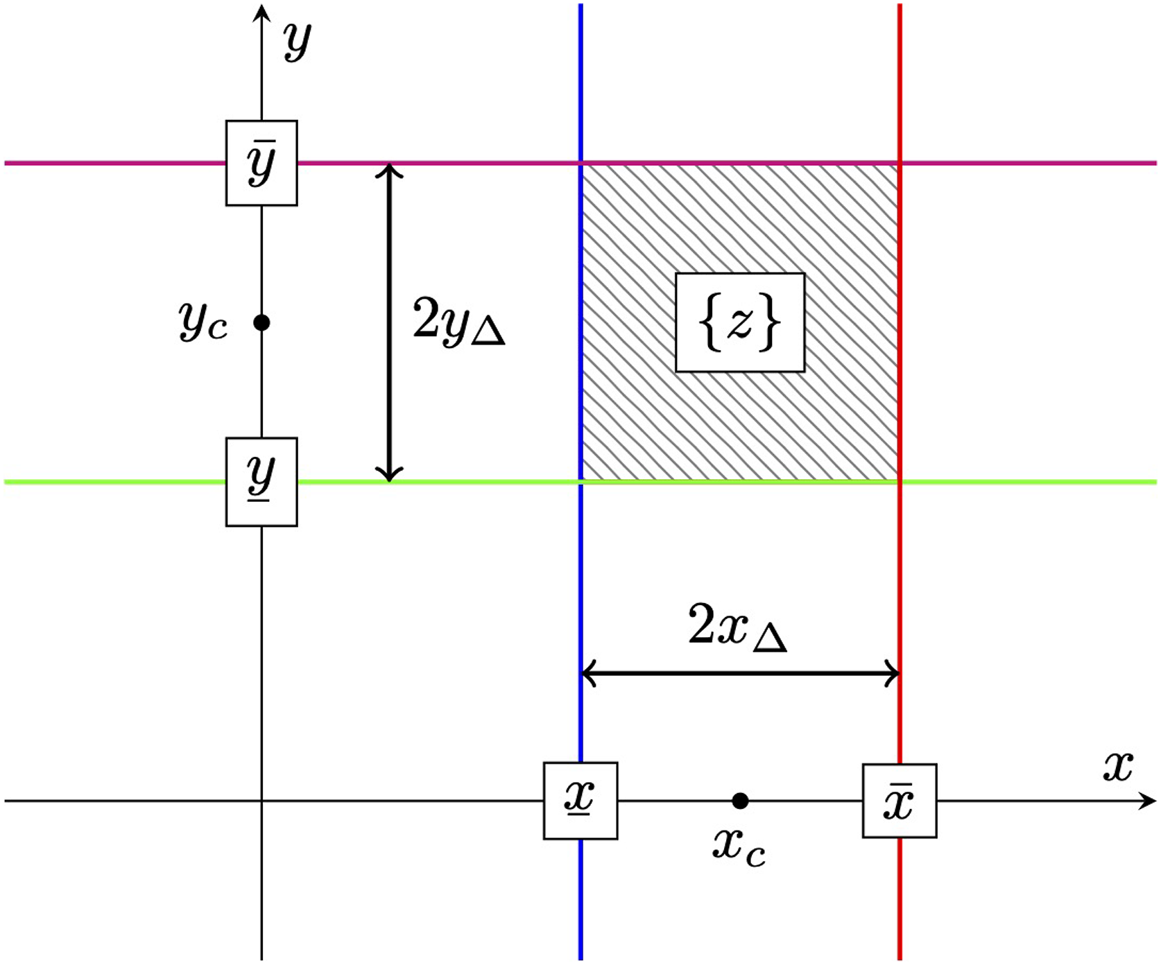

Having defined the notion of a real/complex interval, it is the role of interval analysis to compute the upper and lower bounds of functions whose inputs are intervals

{w} = {u} + i {v} = f ({z_{1}}, {z_{2}}, \dots, {z_{n}}),

(19)

For simple functions, this can be achieved by redefining the basic arithmetic operations + − × ÷ as interval operations ⊕ ⊖ ⊗ ⊘ (Petkovic and Ljiljana, 1998). This leads to the so-called natural interval extension of the function. For more complex problems, global optimisation (Neumaier and Hansen, 1994) or vertex (Dong and Shah, 1987) methods can be used, among other problem specific algorithms.

Care should be taken when using the natural interval extension of a function. Whilst for real intervals the operations ⊕ ⊖ ⊗ ⊘ are optimal (i.e. they provide the smallest possible bounds that enclose the true range of outcomes), this is not so for complex intervals. Specifically, complex division. The natural extension of complex interval division can be expressed as

\begin{array}{l} {x} ⊘ {y} = \\ ({x_{r}} \otimes {y_{r}} \oplus {x_{i}} \otimes {y_{i}}) ⊘ ({y_{r}^{2}} \oplus {y_{i}^{2}}) + \dots \\ i ({x_{i}} \otimes {y_{r}} ⊖ {x_{r}} \otimes {y_{i}}) ⊘ ({y_{r}^{2}} \oplus {y_{i}^{2}}) . \end{array}

(20)

where {x} and {y} are each taken to represent a complex interval. The complex interval obtained as per equation (20) is not optimal.

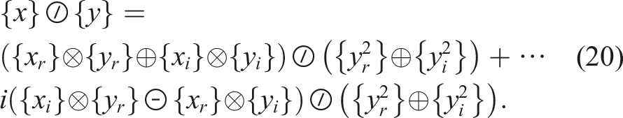
If standard interval arithmetic operations are applied to complex division, the numerator and denominator intervals are treated independently. For example, the instance of {y_r} in the numerator is considered independent to that being squared in the denominator ${y_{r}^{2}}$ . The same issue occurs with {y_i}. This so-called ‘dependency problem’ can lead to a huge overestimation of the interval. Similar dependency issues are often encountered for more complex functions where specific intervals occur more than once and cannot be factored appropriately. This represents one of the main limiting factors of conventional interval arithmetic analysis. For complex division, special algorithms are required to compute the optimal rectangular interval (Rokne and Lancaster, 1971; Lohner and Gudenberg, 1985; Mahmood and Soylu, 2020).

As a final remark on interval analysis, it is noted that non-interval quantities can readily be incorporated within interval arithmetic by considering an interval whose upper and lower bounds are of equal value, x = {x} = [x x].

3.1 Interval sensitivity analysis

Sensitivity analysis (SA) is a tool used to allocate, or apportion, the uncertainty in a system’s output to that of its input parameters (Saltelli et al., 2008). Methods of SA can be broadly categorised as local or global. Local methods assume a small variance on the input parameters and consider a linearisation of the system’s dynamics. Such methods are typically based on partial derivatives (obtained analytically or by numerical approximation). Local methods are advantageous in terms of computational efficiency, but limited in terms of accuracy, especially for non-linear systems with reasonable levels of input variance. Global methods overcome this limitation by sampling the model output over the space of input parameters. Whilst computationally more expensive, this approach ensures that model non-linearity and input parameter distributions are accounted for. Hence, more a robust analysis is achieved.

The local and global methods described above are limited, respectively, by the assumption of linearity and computational efficiency. An alternative approach, overcoming these limitations, is obtained by considering an interval-based SA (Moens and Vandepitte, 2007). Whilst interval SA does not provide a detailed analysis like the global approach, it avoids the need to sample the entire input space; instead of representing each input as a probability distribution, intervals are considered and the bounds of the output are determined.

To illustrate the concept of interval SA we consider the function f( ), whose inputs and output are treated as complex rectangular intervals. We consider the interval output resulting from each input individually

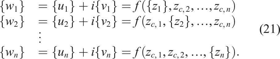
\begin{array}{l} {w_{1}} & = {u_{1}} + i {v_{1}} = f ({z_{1}}, z_{c, 2}, \dots, z_{c, n}) \\ {w_{2}} & = {u_{2}} + i {v_{2}} = f (z_{c, 1}, {z_{2}}, \dots, z_{c, n}) \\ ⋮ \\ {w_{n}} & = {u_{n}} + i {v_{n}} = f (z_{c, 1}, z_{c, 2}, \dots, {z_{n}}) . \end{array}

(21)

Based on equation (21), a measure of sensitivity can be obtained in several ways. Moens and Vandepitte (2007) considered the change in absolute interval widths on the input (z) and the output (w) side of the problem and proposed the sensitivity metric (assuming real valued intervals)

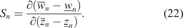
S_{n} = \frac{\partial ({\bar{w}}_{n} - {\underline{w}}_{n})}{\partial ({\bar{z}}_{n} - {\underline{z}}_{n})} .

(22)

For reasons discussed later, in the present paper we choose to define a complex interval sensitivity metric instead as the ratio of output interval area to input interval area

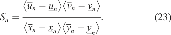
S_{n} = \frac{〈 {\bar{u}}_{n} - {\underline{u}}_{n} 〉 〈 {\bar{v}}_{n} - {\underline{v}}_{n} 〉}{〈 {\bar{x}}_{n} - {\underline{x}}_{n} 〉 〈 {\bar{y}}_{n} - {\underline{y}}_{n} 〉} .

(23)

In this way, S_n describes the relative increase in uncertainty considering the entire range of possible outputs in the complex plane; given the same range of possible inputs, a larger value of S_n indicates a greater range of possible outputs and a greater sensitivity of the function f( ).

The reason for this particular choice of sensitivity metric is that, for the problem considered here (assembly admittance in the presence of joint uncertainty), the output interval takes a very similar form to the Jacobian matrix that describes the partial derivatives of the assembly admittance with respect to joint flexibility. Hence, with this definition of interval sensitivity there is a clear connection to linear/gradient-based SA.

4. Interval assessment of joint variability

In this section we will consider the interval-based assessment of uncertain joint dynamics, and its application in determining the maximum and minimum bounds of an assembled structure’s admittance matrix.

As shown in section 2, the dual formulation, in the presence of a flexible interface, leads to the following equation for the assembled admittance matrix

Y_{C} = Y - Y B^{T} {(B Y B^{T} + Γ)}^{- 1} B Y,

(24)

where the interface flexibility matrix Γ is defined as

\begin{array}{l} Γ = [\begin{matrix} γ_{1} \\ ⋱ \\ γ_{N} \end{matrix}], γ = \frac{1}{k + i r} = γ_{r} + i γ_{i}, \\ γ_{r} = \frac{k}{{| Z |}^{2}}, γ_{i} = - \frac{r}{{| Z |}^{2}} . \end{array}

(25)

With attention focused towards the influence of a single joint, it is convenient to separate its contribution by means of the Sherman–Morrison formula (i.e. a rank-one matrix update) (Hager, 1989)

{(A + X)}^{- 1} = A^{- 1} - \frac{1}{1 + tr (X A^{- 1})} A^{- 1} X A^{- 1},

(26)

where A is any invertible matrix, tr(□) is the trace operator, and X is a matrix of rank one. To apply the Sherman–Morrison formula, the interface flexibility matrix Γ is split into two parts; Γ⁽ⁿ⁾, which contains the nth joint flexibility of interest, and

Γ^{(\tilde{n})}

, which contains all remaining terms

\begin{array}{l} Γ^{(\tilde{n})} = [\begin{matrix} γ_{1} \\ γ_{2} \\ ⋱ \\ 0 \end{matrix}], Γ^{(n)} = [\begin{matrix} 0 \\ 0 \\ ⋱ \\ γ_{n} \end{matrix}] \\ Γ = Γ^{(\tilde{n})} + Γ^{(n)} . \end{array}

(27)

Note that Γ⁽ⁿ⁾ is a rank-one matrix, so can take on the role of X in equation (26). Hence, the matrix inverse in equation (24) can be rewritten in the form

\begin{array}{l} {(B Y B^{T} + Γ^{(\tilde{n})} + Γ^{(n)})}^{- 1} = {(A + Γ^{(n)})}^{- 1} \\ = A^{- 1} - \frac{1}{1 + tr (Γ^{(n)} A^{- 1})} A^{- 1} Γ^{(n)} A^{- 1}, \end{array}

(28)

where

A = B Y B^{T} + Γ^{(\tilde{n})}

. Note that Γ⁽ⁿ⁾ is a single entry matrix. Its only non-zero value, the interface flexibility γ_n, can be brought out as a scalar term, and Γ⁽ⁿ⁾ replaced by P_n, which is a zero matrix bar the nth diagonal entry whose value is one. Equation (28) then reduces to

{(B Y B^{T} + Γ^{(\tilde{n})} + Γ^{(n)})}^{- 1} = A^{- 1} - g_{n} A^{- 1} P_{n} A^{- 1},

(29)

where

g_{n} = \frac{γ_{n}}{1 + tr (P_{n} A^{- 1}) γ_{n}} = \frac{1}{Z_{n} + tr (P_{n} A^{- 1})} = \frac{1}{z_{n}}

(30)

is a complex scalar value, and Z_n = k_n + ir_n is the dynamic stiffness of the nth interface connection. Note that g_n is a non-linear function of γ_n; the joint, although linear in its dynamics, has a non-linear effect on the assembled structure’s admittance matrix. This non-linearity limits the application of local/gradient-based SA. Note that this non-linearity should not be confused with response non-linearity, whereby the structural response is dependent upon the amplitude of said response. Rather, it is system’s coupled admittance matrix that is related non-linearly to the dynamic properties of the joint.

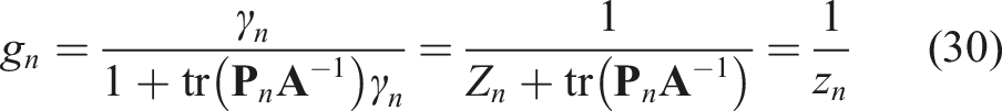
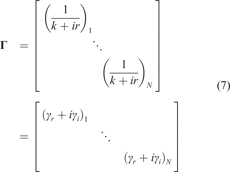
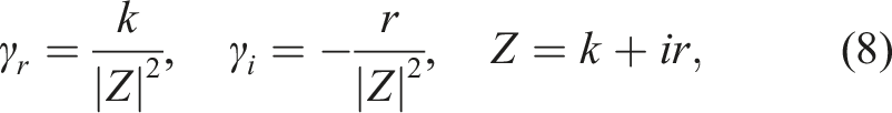
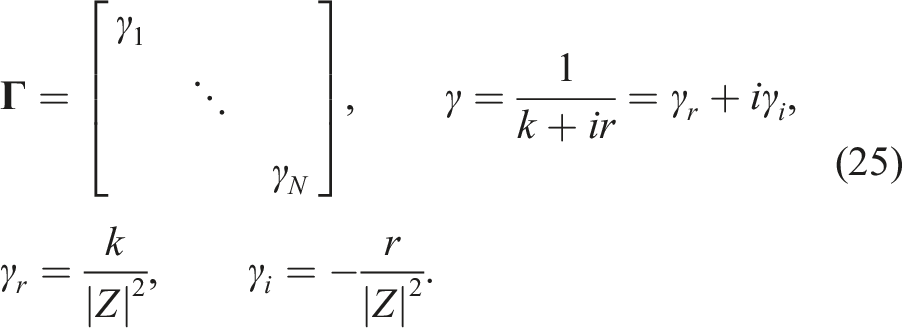
Herein we propose that the interface stiffness Z_n be treated as a complex rectangular interval {Z_n}, such that its bounds are supposed to contain all possible values of joint stiffness and damping. The complex interval {Z} = {k} + i{r} is characterised by a pair of real intervals, namely

{k} = [\underline{k} \bar{k}] = [k_{c} - k_{Δ} k_{c} + k_{Δ}]

(31)

{r} = [\underline{r} \bar{r}] = [r_{c} - r_{Δ} r_{c} + r_{Δ}],

(32)

where

\underline{x}

and

\bar{x}

denote the lower and upper bounds of the respective interval, k_c and r_c are the stiffness and damping mid-points, and k_Δ and r_Δ are the associated half widths.

Treating the interface stiffness as a complex interval {Z_n}, and substituting equations (29) and (30) into equation (24), leads to the interval expression

{Y_{C}} = \overset{Coupled with rigid n}{\overset{⏞}{Y - Y B^{T} {(B Y B^{T} + Γ^{(\tilde{n})})}^{- 1} B Y}} \oplus \underset{Interval matrix describing joint uncertainty}{\underset{⏟}{Y B^{T} {(B Y B^{T} + Γ^{(\tilde{n})})}^{- 1} P_{n} {(B Y B^{T} + Γ^{(\tilde{n})})}^{- 1} B Y ⊘ {z_{n}}}}

(33)

{Y_{C}} = Y_{C}^{(\tilde{n})} \oplus {Δ Y_{C}^{(n)}},

(34)

where

{z_{n}} = {Z_{n}} \oplus tr (P_{n} A^{- 1})

, and {Y_C} is a complex interval admittance matrix whose bounds enclose all possible values obtainable given the range of permissible joint dynamics specified by the interval {Z_n}.

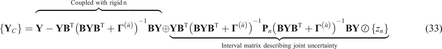
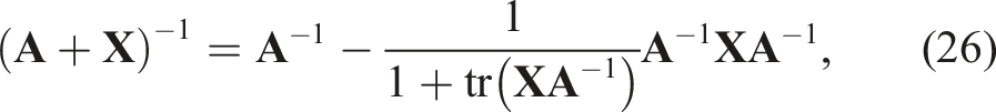
It is important that the complex interval division of equation (33) is performed optimally using an appropriate algorithm. Unlike complex addition, subtraction and multiplication, the natural interval extension of complex division is not optimal and can lead to a large overestimation of the resulting bound (Rokne and Lancaster, 1971; Lohner and Gudenberg, 1985; Mahmood and Soylu, 2020). In the present paper, we propose an application specific algorithm (see Appendix B) to obtain the precise bounds of the complex interval {Y_C} (also the magnitude interval {|Y_C|}).

Note that $Y_{C}^{(\tilde{n})}$ contains no intervals, and represents the structure’s admittance when γ_n = 0, that is, when the nth connection is made rigid. Hence, ${Δ Y_{C}^{(n)}}$ represents an interval matrix that describes the effect, or influence, of the nth joint’s relaxation on the coupled admittance.

It is further noted that the matrix product within ${Δ Y_{C}^{(n)}}$ represents the assembly’s Jacobian matrix, J_n, with respect to the interface flexibility γ_n, evaluated for a rigid connection (see Appendix A)

\begin{array}{l} J_{n} = {[\begin{matrix} \frac{\partial Y_{11}}{\partial γ_{n}} \dots \frac{\partial Y_{1 N}}{\partial γ_{n}} \\ ⋮ ⋱ ⋮ \\ \frac{\partial Y_{N 1}}{\partial γ_{n}} \dots \frac{\partial Y_{N N}}{\partial γ_{n}} \end{matrix}]}_{γ_{n} = 0} \\ = Y B^{T} {(B Y B^{T} + Γ^{(\tilde{n})})}^{- 1} P_{n} {(B Y B^{T} + Γ^{(\tilde{n})})}^{- 1} B Y . \end{array}

(35)

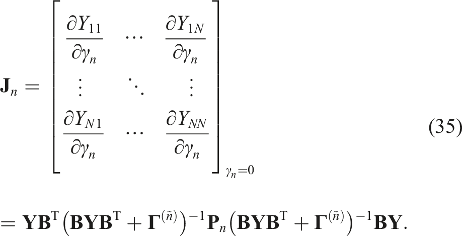
This Jacobian matrix would form the basis of a local/gradient-based SA (Meggitt, 2022). From the above, it is clear that ${Δ Y_{C}^{(n)}}$ is proportional to the system Jacobian, but includes the interval contribution of the uncertain joint through the interval term {z}. It is for this reason that we choose to define interval sensitivity as per equation (23), as opposed to the derivative of the interval width as per equation (22) (Moens and Vandepitte, 2007).

4.1 Response interval

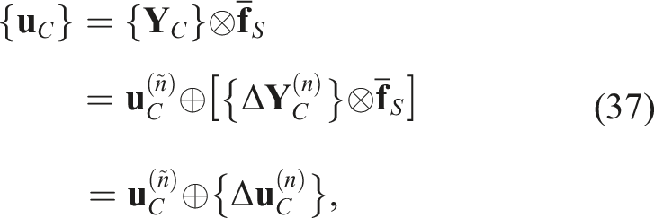
In the presence of an active component (i.e. a vibration source) the operational response u_C is often of greater importance than the assembly admittance. Hence, we look to extend the interval treatment above to account for an assembly’s operational activity.

The operational response of a complex assembly can be expressed in the form

u_{C} = Y_{C} {\bar{f}}_{S},

(36)

where Y_C is the coupled admittance matrix, and

{\bar{f}}_{S}

is a vector of so-called blocked forces (Moorhouse et al., 2009). The blocked force is an independent source quantity that describes its operational activity. It has become an internationally standardised method for experimentally characterising vibratory sources (International Organization for Standardization, 2019), and is used extensively across several engineering sectors, including automotive (Elliott et al., 2013; Lennström et al., 2016), railway (Elliott et al., 2019; Sanei et al., 2019), heavy machinery (Cabaret et al., 2020) and building acoustics (Patil et al., 2017).

As per equation (36), the complex interval of an operational response can be obtained by

\begin{matrix} {u_{C}} = {Y_{C}} \otimes {\bar{f}}_{S} \\ = u_{C}^{(\tilde{n})} \oplus [{Δ Y_{C}^{(n)}} \otimes {\bar{f}}_{S}] \\ = u_{C}^{(\tilde{n})} \oplus {Δ u_{C}^{(n)}}, \end{matrix}

(37)

where it is noted that ⊗ represents an interval matrix multiplication. Like the assembly admittance, the interval response is made up of two parts; the first is that of the assembly when the nth joint is considered rigid

u_{C}^{(\tilde{n})}

, and the second is an interval contribution describing a relaxation of the nth joint

{Δ u_{C}^{(n)}}

5. Numerical example

In this section we will demonstrate the interval SA for joint dynamics through a numerical example. The system considered is illustrated in Figure 3. It is an 11 DoF mass-spring-damper system (numeric values are available via the supplementary MATLAB codes). It comprises two sub-systems (green and blue) connected by three joint elements (red), whose properties are considered uncertain.

Figure 3.

Numerical mass-spring example.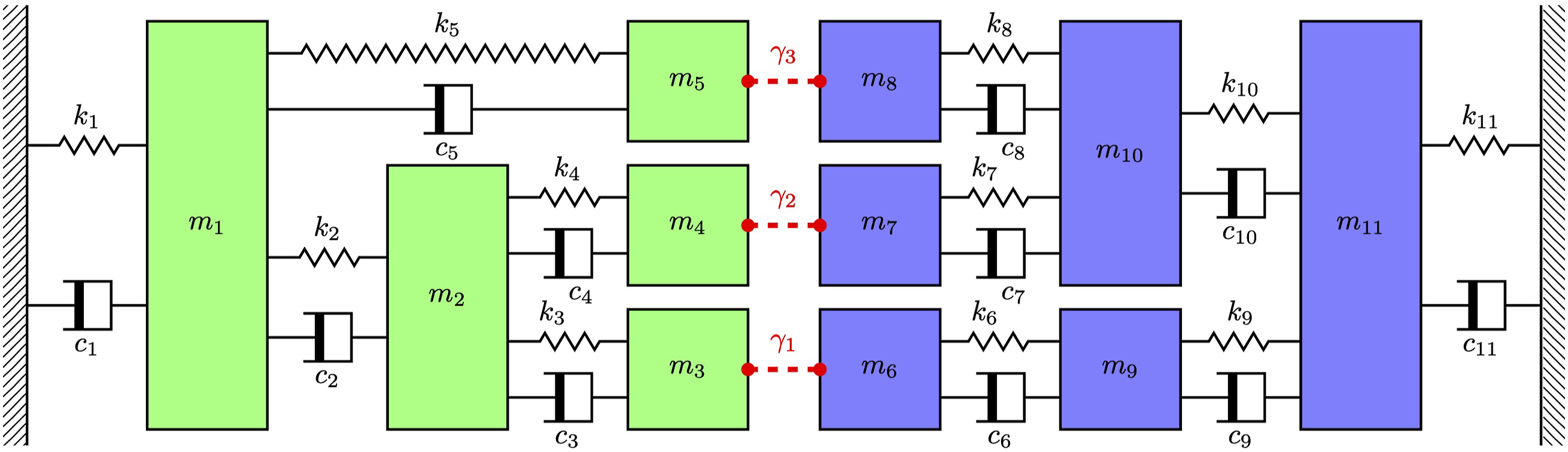

In this numerical example we will (a) for a single joint, demonstrate the interval computation for the real, imaginary and magnitude admittance bounds, and compare the results against those obtained by a sample-based estimation, and (b) rank order the uncertainty contribution of each joint towards the assembly admittance using the proposed sensitivity metric.

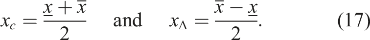
In what follows, each joint is represented by its centre point stiffness and damping, and parametrised by an uncertainty factor α_□ = □_Δ/□_c which controls the width of the interval bound

{k_{n}} = [(1 - α_{k, n}) k_{c, n} (1 + α_{k, n}) k_{c, n}]

(38)

{r_{n}} = [(1 - α_{r, n}) r_{c, n} (1 + α_{r, n}) r_{c, n}],

(39)

Unless otherwise stated, the centre point stiffness and damping values are set at 1 × 10⁴ (N/m) and 100 (Ns/m), respectively, with uncertainty factors α _k,n = 0.5 and α _r,n = 0.25.

To validate the interval computation a sample-based estimate is used. The complex joint interval ${Z_{n}} = [\underline{k} \bar{k}] + i [\underline{r} \bar{r}]$ is logarithmically sampled between the lower and upper bounds of its real and imaginary parts, generating a total of n = 100² sample points per frequency. These samples are used to compute n complex admittance matrices, the max/min values of which are taken as estimates of the complex interval {Y_C}. The magnitude of each complex admittance is also taken to estimate {|Y_C|}.

We begin by considering the interval bounds due to a single joint; joint 1 is represented by the complex interval {Z₁}, whilst joints 2 and 3 are considered deterministic (α_k,2 = α_k,3 = 0, α_r,2 = α_r,3 = 0).

Shown in Figure 4 are the interval bounds of the real and imaginary parts of the complex admittance ${Y_{C_{1,11}}}$ . Orange markers denote the sample-based estimates and solid lines the interval computations obtained as per the algorithm described in Appendix B. To plot the intervals on a logarithmic scale, magnitudes are taken for both the real and imaginary parts; positive values are shown in blue, and negative values in green.

Figure 4.

Interval bounds for the real (top) and imaginary (bottom) admittance 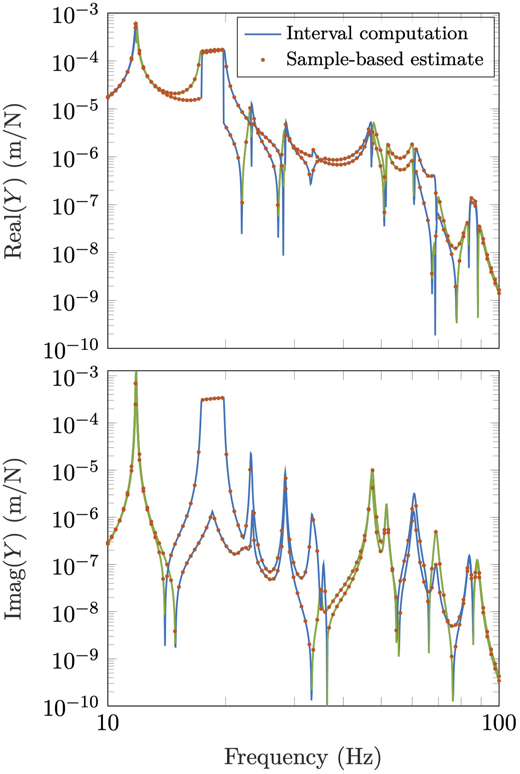${Y_{C_{1,11}}}$ due to complex joint interval {Z₁}. Sample-based estimates are shown by orange markers and interval computations by blue plots (green plots indicate frequency ranges where the value <0).

It is clear from Figure 4 that the interval computation (see Appendix B) correctly determines the bounds on both the real and imaginary admittance. These bounds will be used shortly to compute the interval sensitivity metric, as per equation (40).

Shown in Figure 5 are the magnitude bounds of the complex admittance ${| Y_{C_{1,11}} |}$ . Also shown, in black, is the mid-point response, obtained by considering k₁ = k_c,1 and r₁ = r_c,1. As expected, we see that the interval computation successfully captures the shifts in resonant and anti-resonant frequencies due to the unknown interface flexibility; this is particularly evident around 19 Hz where the second system resonance varies between 17–20 Hz.

Figure 5.

Interval bounds of admittance magnitude 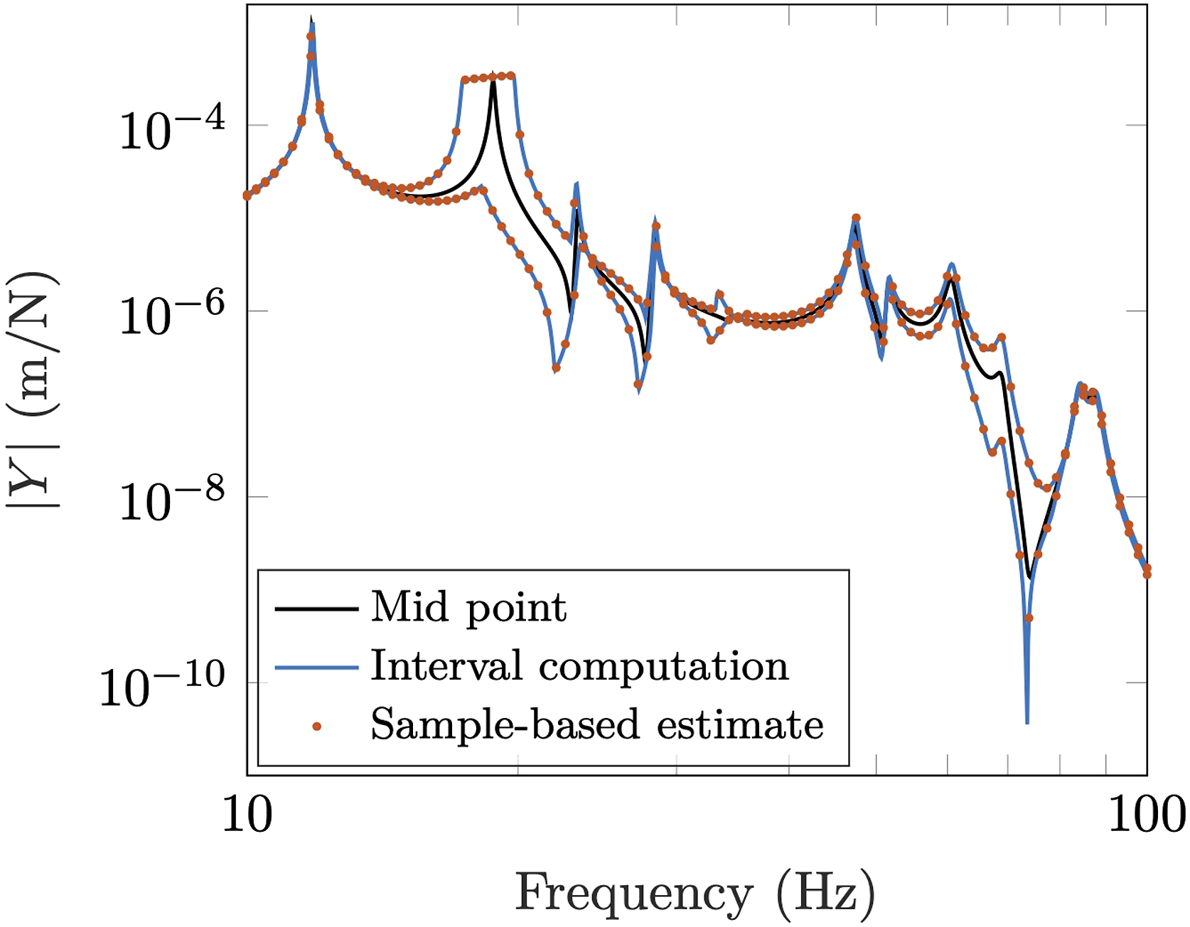${| Y_{C_{1,11}} |}$ due to the complex joint interval {Z₁}. Sample-based estimates are shown by orange markers and interval computations by blue plots. The mid-point admittance is shown in black.

It is interesting to note that the lower bound of the $\approx 70$ Hz anti-resonance, goes to zero (hence cannot be plotted). This indicates that there exists a combination of joint stiffness and damping that yields zero transmission through the interface.

Figures 4 and 5 provide a visual indication of the sensitivity of the assembly admittance with respect to joint 1. It is clear that the certain modes have a greater sensitivity to joint uncertainty than others.

5.1 Interval sensitivity analysis

With attention focused towards the influence of joint uncertainty, our definition of complex interval sensitivity (see equation (23)) takes the form

S_{n} = \frac{〈 Re (Δ {\bar{Y}}_{C_{i, j}}^{(n)}) - Re (Δ {\underline{Y}}_{C_{i, j}}^{(n)}) 〉 〈 Im (Δ {\bar{Y}}_{C_{i, j}}^{(n)}) - Im (Δ {\underline{Y}}_{C_{i, j}}^{(n)}) 〉}{〈 Re ({\bar{Z}}_{n}) - Re ({\underline{Z}}_{n}) 〉 〈 Im ({\bar{Z}}_{n}) - Im ({\underline{Z}}_{n}) 〉},

(40)

where Z_n = k_n + i r_n is the joint dynamic stiffness, and

Δ Y_{C_{i, j}}^{(n)}

describes the dynamic contribution of the nth joint.

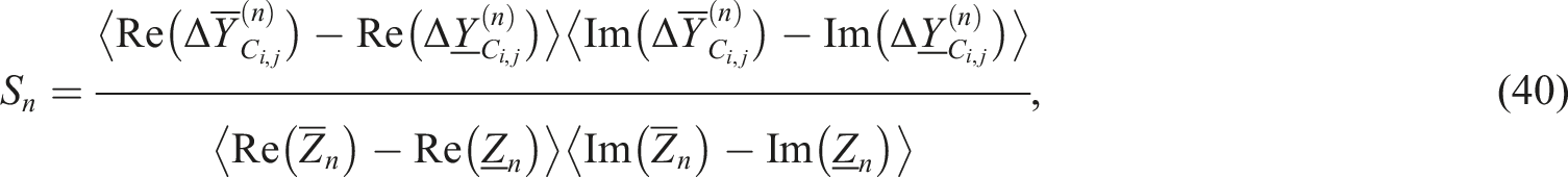
The sensitivity S_n describes the relative amplification of uncertainty in terms of the complex interval areas that describe the joint and coupled admittance. The greater the metric, the greater the influence that joint has on the assembly admittance. By comparing the sensitivity metric of each joint it is possible to identify the dominant source of uncertainty in the system. For clarity, we present all sensitivity metrics in a normalised form

{\hat{S}}_{n} = \frac{S_{n}}{\sum_{i} S_{i}},

(41)

where a value of approx. 1 indicates that the uncertainty of the assembly admittance is almost entirely due to the nth joint. Similarly, a value of approx. 0 indicates that the joint contributes negligibly to the admittance uncertainty.

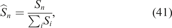
It should be noted that the sensitivity metric considers the influence of each joint independently (remaining joints are treated as deterministic with centre point stiffness and damping); interaction effects between multiple joints are not considered.

Shown in Figure 6 are the magnitude interval bounds with respect to each uncertain joint (taking α _k,n = 0.5, α _r,n = 0.25), alongside their corresponding (normalised) sensitivity metrics. For clarity, sample-based estimates have been omitted. Figure 7 similarly presents the magnitude interval and sensitivity metrics for the reduced uncertainty levels of α _k,n = 0.05 and α _r,n = 0.025.

Figure 6.

Interval bounds of the admittance magnitude (top) considering each joint’s interval uncertainty individually, and the corresponding interval sensitivity metrics (bottom). Mid-point admittance shown in black. Uncertainty factors: α_k,n = 0.05, α_r,n = 0.025.

Figure 7.

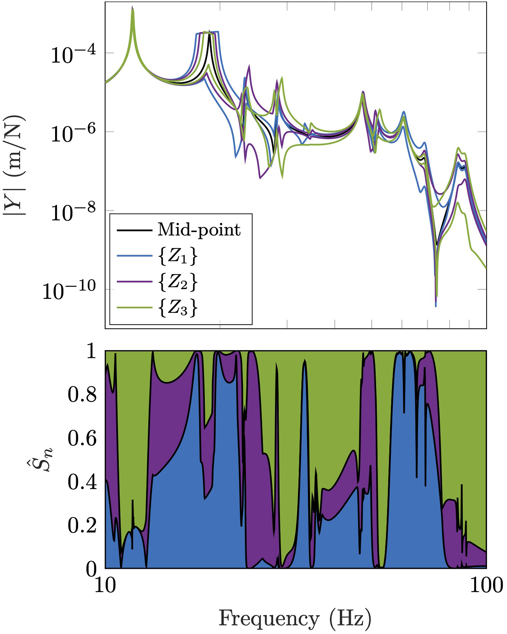
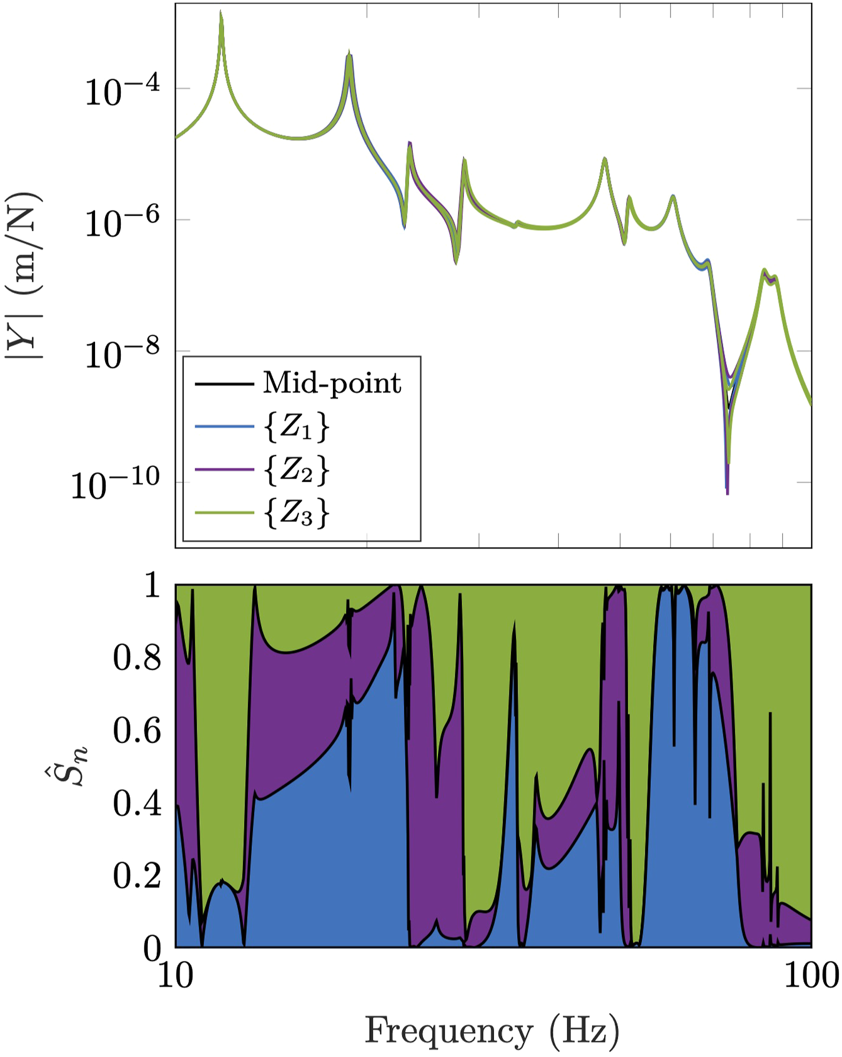
The relative widths of the magnitude bounds provide a visual indication of the influence of each uncertain joint, though their respective sensitivities depend also on the relative size of the input interval; this cannot be interpreted from the magnitude bounds alone. Rather, the sensitivity metric ${\hat{S}}_{n}$ provides an indication of the relative increase in uncertainty by comparing the input and output interval areas for each joint. Though a rank ordering, this result can be used to aid model refinement, by targeting those joints with the greatest sensitivity. From Figure 6, we might conclude that above approx 50 Hz, joints 1 and 3 have the greatest sensitivity, whilst below 50 Hz joints 1 and 2 appear to dominate.

Careful comparison of the sensitivity metrics presented in Figures 6 and 7 uncover an interesting result. The sensitivity with respect to a particular joint depends on the size of the input interval; the sensitivity metric captures the non-linear contribution of the uncertain joint’s dynamics towards the system response (which arises due to equation (30)). Though only a minor effect in the present case study, more complex systems can exhibit much greater effects (Meggitt, 2022). This ability to capture non-linear behaviour is a principal advantage of interval-based SA over conventional gradient-based methods, which rely on a linearisation of the system dynamics.

For more complex systems, the sensitivities of several joints can be combined to form a single sensitivity value. For example, the stiffness and damping in each coordinate direction (x, y, z) for a single connection point might be combined to yield a sensitivity value for the connection as a whole (Meggitt, 2022).

6. Conclusions

Joints are a principal source of uncertainty when modelling the dynamics of complex built-up structures. To better understand their influence, it is of interest to apportion the uncertainty of a system’s output (FRF or operational response) to that of its uncertain joint dynamics by means of sensitivity analysis (SA). To overcome the limitations of conventional ‘probabilistic’ SA, we have proposed an interval-based SA for joint dynamics in complex built-up structures.

We introduce an application-specific algorithm that enables precise bounds on the real, imaginary and magnitude admittance to be determined, based on the interval uncertainty of each joint. To characterise the sensitivity of the system to a particular joint, we propose a complex interval sensitivity metric, representing a ratio of complex interval areas on the input and output of the system. This metric indicates the relative increase or decrease in uncertainty, in an interval sense, due to the dynamics of the system. This metric can be used to identify those joints that contribute unacceptably to the total uncertainty of the system, for example, for model refinement purposes.

The advantages of the proposed interval SA, over conventional (probabilistic) local and global methods are many:

1) As per the interval paradigm, there is no need for a detailed probabilistic description of each joint, which is often unavailable. Rather, only the upper and lower limits of joint stiffness and damping are required.

2) The interval SA is not limited to the linear behaviour of the system (as per local gradient-based methods); all system non-linearities contained within the input interval bounds are accounted for; hence, the method can be termed ‘pseudo-global’. The ability of interval SA to capture the system’s non-linear dependence on the joint dynamics was demonstrated by numerical example, where it was shown that the sensitivity metric provided a different rank ordering when subject to different levels of input uncertainty.

3) Unlike standard global methods, which sample the input parameter space over their probabilistic representations, the proposed interval SA is computed analytically, and so avoids the computational burden of sampling over a multi-dimension input space.

Though, a notable limitation of the proposed interval SA is its inability to treat multiple joints at a time, both in terms of uncertainty propagation (obtaining the admittance bounds) and SA. Consequently, the interaction between multiple uncertain joints cannot be accounted for, nor can the admittance bounds due to several uncertain joints be determined. Extension of the proposed interval SA to the multi-joint case was considered beyond the scope of this paper, and is left as further work.

Footnotes

Declaration of conflicting interests

The author(s) declared no potential conflicts of interest with respect to the research, authorship, and/or publication of this article.

Funding

The author(s) received no financial support for the research, authorship, and/or publication of this article.

ORCID iD

Joshua WR Meggitt

Supplementary material

All MATLAB codes are available on request.

Jacobian of the coupled admittance

In this section we derive the Jacobian matrix for the coupled admittance with respect to a specific joint flexibility.

We begin by considering the complex differential of the assembly admittance (42)

d Y_{C} = d (Y) - d (Y B^{T} {(B Y B^{T} + Γ)}^{- 1} B Y) .

Noting that interest lies in the differential interface flexibility d(Γ), the above reduces to (43)

d Y_{C} = - d (Y B^{T} {(B Y B^{T} + Γ)}^{- 1} B Y) .

Application of the product rule, $d (A B C) = d (A) B C + A d (B) C + A B d (C)$ , then leads to (44)

d Y_{C} = - Y B^{T} d {(B Y B^{T} + Γ)}^{- 1} B Y .

Recalling the differential of a matrix inverse (Hjørungnes, 2013), $d {(A)}^{- 1} = - A^{- 1} d (A) A^{- 1}$ , yields (45)

\begin{array}{l} d Y_{C} = Y B^{T} {(B Y B^{T} + Γ)}^{- 1} & d (B Y B^{T} + Γ) \dots \\ {(B Y B^{T} + Γ)}^{- 1} B Y \end{array}

which reduces to (46)

d Y_{C} = Y B^{T} {(B Y B^{T} + Γ)}^{- 1} d (Γ) {(B Y B^{T} + Γ)}^{- 1} B Y .

In equation (46), we can interpret dY_C as the small (complex) change in admittance, due to a small (complex) change in the interface flexibility $d (Γ)$ . Importantly, $d (Γ)$ represents a small change in each matrix entry. Focussing attention on the nth interface connection in particular, such that $d (Γ) \to P_{n} d γ_{n}$ , where P_n is a zero matrix bar the nth diagonal entry, whose value is one, equation (46) becomes (47)

\begin{array}{l} d Y_{C} & = Y B^{T} {(B Y B^{T} + Γ)}^{- 1} P_{n} \dots {(B Y B^{T} + Γ)}^{- 1} B Y d γ_{n} \\ = J_{n} d γ_{n}, \end{array}

where dγ_n is a scalar differential of the nth interface flexibility, and J_n is a complex Jacobian matrix containing the partial derivatives of the coupled assembly admittance, with respect to the nth interface flexibility (48)

J_{n} = [\begin{matrix} \frac{\partial Y_{11}}{\partial γ_{n}} & \dots & \frac{\partial Y_{1 N}}{\partial γ_{n}} \\ ⋮ & ⋱ & ⋮ \\ \frac{\partial Y_{N 1}}{\partial γ_{n}} & \dots & \frac{\partial Y_{N N}}{\partial γ_{n}} \end{matrix}] .

The Jacobian is evaluated for a specific value of interface flexibility by setting the elements of Γ as necessary.

Interval computation

In this section we describe the computation of the complex interval admittance {Y_C}, and its interval magnitude {|Y_C|}. A MATLAB implementation of the interval computation described below is available on request.

For a single interval joint, the complex interval admittance is given by (see equations (33)–(35)) (49)

{Y_{C}} = Y_{C}^{(\tilde{n})} \oplus (J_{n} ⊘ {z_{n}}) .

Taking the ijth element of the admittance, Y_C,ij, we are interested in evaluating a complex interval of the form (50)

{Y_{C, i j}} = Y_{C, i j}^{(\tilde{n})} \oplus (J_{n, i j} ⊘ {z_{n}}) = Y_{C, i j}^{(\tilde{n})} \oplus {w_{n, i j}} .

Omitting subscripts for clarity, we begin by considering the bounds of the complex interval {w}.

With z = x + iy and J = a + ib, we have (51)

w = u + i v = \frac{a + i b}{x + i y} .

Rearranging the above we obtain equations for the real and imaginary parts of z (52)

x = \frac{a u + b v}{u^{2} + v^{2}}, y = \frac{b u - a v}{u^{2} + v^{2}} .

To represent the intervals ${x} = [\underline{x} \bar{x}]$ and ${y} = [\underline{y} \bar{y}]$ , we consider the following inequalities: (53)

\begin{array}{l} \frac{a u + b v}{u^{2} + v^{2}} > \underline{x}, \frac{a u + b v}{u^{2} + v^{2}} < \bar{x} \end{array}

(54)

\begin{array}{l} \frac{b u - a v}{u^{2} + v^{2}} > \underline{y}, \frac{b u - a v}{u^{2} + v^{2}} < \bar{y} \end{array} .

Taking the $\underline{x}$ inequality, and rearranging, yields (55)

{(u - \frac{a}{2 \underline{x}})}^{2} + {(v - \frac{b}{2 \underline{x}})}^{2} < {(\frac{a}{2 \underline{x}})}^{2} + {(\frac{b}{2 \underline{x}})}^{2}

which represents a closed (since <) circular domain in the (u, v) plane with centre point

(\frac{a}{2 \underline{x}}, \frac{b}{2 \underline{x}})

and radius

r = \sqrt{{(\frac{a}{2 \underline{x}})}^{2} + {(\frac{b}{2 \underline{x}})}^{2}}

. Similarly, the

\bar{x}

\underline{y}

and

\bar{y}

inequalities yield: (56)

\begin{array}{l} {(u - \frac{a}{2 \bar{x}})}^{2} + {(v - \frac{b}{2 \bar{x}})}^{2} > {(\frac{a}{2 \bar{x}})}^{2} + {(\frac{b}{2 \bar{x}})}^{2} \end{array}

(57)

\begin{array}{l} {(u - \frac{b}{2 \underline{y}})}^{2} + {(v + \frac{a}{2 \underline{y}})}^{2} < {(\frac{a}{2 \underline{y}})}^{2} + {(\frac{b}{2 \underline{y}})}^{2} \end{array}

(58)

\begin{array}{l} {(u - \frac{b}{2 \bar{y}})}^{2} + {(v + \frac{a}{2 \bar{y}})}^{2} > {(\frac{a}{2 \bar{y}})}^{2} + {(\frac{b}{2 \bar{y}})}^{2} \end{array}

which represent open, closed and open circular domains, respectively. Note that the direction of the inequalities (i.e. whether they are open or closed) depends on the relative sign of

\underline{x}

\bar{x}

\underline{y}

, and

\bar{y}

The intersection of the four domains describes a conformal mapping from the complex plane z = x + iy (specifically, the complex rectangular interval {z}), to the domain of w = u + iv. An example is illustrated in Figure 8. The complex interval {w} represents the smallest rectangle that encloses the domain w. Figure 8.

Conformal map f(z) = J/z applied to the open regions 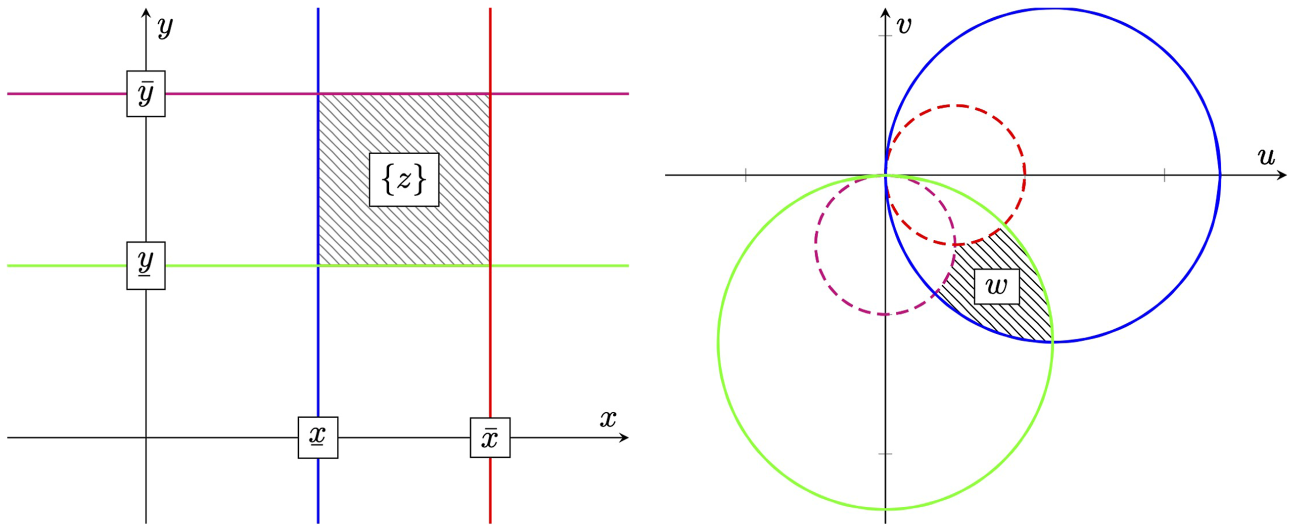$x > \underline{x}$ (blue), $x < \bar{x}$ (red), $y > \underline{y}$ (green), and $y < \bar{y}$ (magenta). In the u/v plane, solid lines denote closed domains, and dashed lines open domains. The patterned intersection represents the conformal mapping of the complex interval {z}; the complex interval {w} is described by the smallest rectangle that encloses w.

The subsequent addition of $Y_{C}^{(\tilde{n})}$ in equation (50) acts to translate each domain in the complex plane. This is equivalent to translating the centre points of each circular domain, for example, (59)

(\frac{a}{2 x}, \frac{b}{2 x}) \to (\frac{a}{2 x} + real (Y_{C}^{(\tilde{n})}), \frac{b}{2 x} + imag (Y_{C}^{(\tilde{n})})) .

Hence, evaluation of the complex interval admittance {Y_C} reduces to finding the smallest enclosing rectangle that surrounds the intersection of the translated circular domains described above.

An estimate of magnitude interval admittance {|Y_C|} can subsequently be found by considering each vertex of the complex rectangularinterval {Y_C}, taking smallest/largest absolute distance from the origin as the minimum/maximum interval bound. However, for certain combinations of J and z this can lead to a large over estimation of the true magnitude bound, as the complex (rectangular) interval {Y_C} naturally encloses regions that lie outside the true domain of Y_C. An alternative approach considers the relative size of each circular domain and finds the precise magnitude bounds. This approach is detailed in the following subsection.

References

Ben-Haim

Elishakoff

(2013) Convex models of uncertainty in applied mechanics. Elsevier.

Cabaret

Elliott

Farrell

, et al. (2020) Prediction of structure borne noise and vibration for resiliently coupled equipment using blocked forces and substructuring. Proceedings of ISMA 2018-International Conference on Noise and Vibration Engineering and USD 2018-International Conference on Uncertainty in Structural Dynamics.

Čelič

Boltežar

(2008) Identification of the dynamic properties of joints using frequency-response functions. Journal of Sound and Vibration 317(1–2): 158–174. DOI: 10.1016/j.jsv.2008.03.009.

Chen

Rao

(1997) Fuzzy finite-element approach for the vibration analysis of imprecisely-defined systems. Finite Elements in Analysis and Design 27(1): 69–83. DOI: 10.1016/S0168-874X(97)00005-X.

Chen

Lian

Yang

, et al. (2003) Interval eigenvalue analysis for structures with interval parameters. Finite Elements in Analysis and Design 39(5–6): 419–431. DOI: 10.1016/S0168-874X(02)00082-3.

Chen

Meng

, et al. (2009) An efficient method for evaluating the natural frequencies of structures with uncertain-but-bounded parameters. Computers and Structures 87(9–10): 582–590. DOI: 10.1016/j.compstruc.2009.02.009.

De Klerk

Rixen

Voormeeren

, et al. (2008) General framework for dynamic substructuring: history, review, and classification of techniques. AIAA Journal 46(5): 1169–1181. DOI: 10.2514/1.33274.

de Oliveira Teloli

Villani

LGG

da Silva

, et al. (2021) On the use of the GP-NARX model for predicting hysteresis effects of bolted joint structures. Mechanical Systems and Signal Processing 159: 107751. DOI: 10.1016/j.ymssp.2021.107751.

Dong

Shah

(1987) Vertex method for computing functions of fuzzy variables. Fuzzy Sets and Systems 24(1): 65–78. DOI: 10.1016/0165-0114(87)90114-X.

10.

Elliott

Moorhouse

Huntley

, et al. (2013) In-situ source path contribution analysis of structure borne road noise. Journal of Sound and Vibration 332(24): 6276–6295.

11.

Elliott

Moorhouse

Sanei

, et al. (2019) INTER-NOISE 2019 MADRID - 48th International Congress and Exhibition on Noise Control Engineering.Structure borne noise characterization of an air generation and treatment unit (AGTU) for a train using the mobility method and sub-structuring.

12.

Ewins

(1984) Modal Testing: Theory and Practice (Mechanical Engineering Research Studies).

13.

Faes

Moens

(2020) Recent Trends in the Modeling and Quantification of Non-probabilistic Uncertainty, Volume 27. Springer Netherlands. DOI: 10.1007/s11831-019-09327-x.

14.

Fujita

Takewaki

(2011) An efficient methodology for robustness evaluation by advanced interval analysis using updated second-order Taylor series expansion. Engineering Structures 33(12): 3299–3310. DOI: 10.1016/j.engstruct.2011.08.029.

15.

Hager

(1989) Updating the inverse of a matrix. SIAM Review 31(2): 221–239. DOI: 10.1137/1031049.

16.

Hjørungnes

(2013) Complex-Valued Matrix Derivatives, Volume 369. 1st edition. New York: Cambrudge University Press. DOI: 10.1017/CBO9781107415324.004.

17.

Ibrahim

Pettit

(2005) Uncertainties and dynamic problems of bolted joints and other fasteners. Journal of Sound and Vibration 279(3–5): 857–936. DOI: 10.1016/j.jsv.2003.11.064.

18.

Imholz

Faes

Vandepitte

, et al. (2020) Robust uncertainty quantification in structural dynamics under scarse experimental modal data: a Bayesian-interval approach. Journal of Sound and Vibration 467: 114983. DOI: 10.1016/j.jsv.2019.114983.

19.

International Organization for Standardization (1994) Experimental Determination of mechanical mobility - Part 5: Measurement using Impact Excitation with an Exciter Which Is Not attached to the Structure. BS 6897-5 1995, ISO 7626-5 1994.

20.

International Organization for Standardization (2019) Acoustics - Characterization of Sources of Structure-Borne Sound and Vibration - Indirect Measurement of Blocked Forces. ISO 20270:2019.

21.

Langley

(2000) Unified approach to probabilistic and possibilistic analysis. Journal of Engineering Mechanics 126(November): 1163–1172.

22.

Łasecka-Plura

Lewandowski

(2017) Dynamic characteristics and frequency response function for frame with dampers with uncertain design parameters. Mechanics Based Design of Structures and Machines 45(3): 296–312. DOI: 10.1080/15397734.2017.1298043.

23.

Lei

Yaru

Yisi

, et al. (2019) An inverse method for distributed dynamic load identification of structures with interval uncertainties. Advances in Engineering Software 131(January): 77–89. DOI: 10.1016/j.advengsoft.2019.02.003.

24.

Lennström

Olsson

Wullens

, et al. (2016) Validation of the blocked force method for various boundary conditions for automotive source characterization. Applied Acoustics 102(JANUARY): 108–119. DOI: 10.1016/j.apacoust.2015.08.019.

25.

Lohner

Gudenberg

JWV

(1985) Complex interval division with maximum accuracy. In: Proceedings - Symposium on Computer Arithmetic. pp. 332–336. DOI: 10.1109/ARITH.1985.6158963.

26.

Mahmood

EMN

Soylu

(2020) An effective method for division of rectangular intervals. AIMS Mathematics 5(6): 6355–6372. DOI: 10.3934/math.2020409.

27.

Marques

Flores

Claro

JCP

, et al. (2016) A survey and comparison of several friction force models for dynamic analysis of multibody mechanical systems. Nonlinear Dynamics 86(3): 1407–1443. DOI: 10.1007/s11071-016-2999-3.

28.

Meggitt

(2022) Interval-based identification of response-critical joints in complex built-up structures : a tool for model refinement. Journal of Sound and Vibration 529: 1–28.

29.

Moens

Vandepitte

(2004) An interval finite element approach for the calculation of envelope frequency response functions. International Journal for Numerical Methods in Engineering 61(14): 2480–2507. DOI: 10.1002/nme.1159.

30.

Moens

Vandepitte

(2007) Interval sensitivity theory and its application to frequency response envelope analysis of uncertain structures. Computer Methods in Applied Mechanics and Engineering 196(21–24): 2486–2496. DOI: 10.1016/j.cma.2007.01.006.

31.

Moorhouse

Elliott

Evans

, et al. (2009) In situ measurement of the blocked force of structure-borne sound sources. Journal of Sound and Vibration 325(4–5): 679–685. DOI: 10.1016/j.jsv.2009.04.035.

32.

Muscolino

Santoro

Sofi

, et al. (2014) Explicit frequency response functions of discretized structures with uncertain parameters. Computers and Structures 133: 64–78. DOI: 10.1016/j.compstruc.2013.11.007.

33.

Muscolino

Sofi

(2012) Stochastic analysis of structures with uncertain-but-bounded parameters via improved interval analysis. Probabilistic Engineering Mechanics 28: 152–163. DOI: 10.1016/j.probengmech.2011.08.011.

34.

Muscolino

Sofi

(2013) Bounds for the stationary stochastic response of truss structures with uncertain-but-bounded parameters. Mechanical Systems and Signal Processing 37(1–2): 163–181. DOI: 10.1016/j.ymssp.2012.06.016.

35.

Neumaier

Hansen

(1994) Global Optimization Using Interval Analysis Volume 63. DOI: 10.2307/2153591.

36.

Noll

Dreyer

Singh

, et al. (2013) Identification of dynamic stiffness matrices of elastomeric joints using direct and inverse methods. Mechanical Systems and Signal Processing 39(1–2): 227–244. DOI: 10.1016/j.ymssp.2013.02.003.

37.

Patil

Elliott

Moorhouse

(2017) A blocked pressure based transfer path analysis (TPA) method to measure the sound insulation path contributions of a partition subjected to an incident airborne field. 24th International Congress on Sound and Vibration, ICSV 2017: 1–8.

38.

Petkovic

Ljiljana

(1998) Complex Interval Arithmetic and its Applications. WILEY-VCH.

39.

Petyt

(2010) Introduction to Finite Element Vibration analysis. 2nd edition. New York: Cambridge University Press.

40.

Rao

Berke

(1997) Analysis of uncertain structural systems using interval analysis. AIAA Journal 35(4): 727–735.

41.

Ren

Beards

(1995) Identification of joint properties of a structure using FRF data. Journal of Sound and Vibration 186(4): 567–587. DOI: 10.1006/jsvi.1995.0469.

42.

Ren

Beards

(1998) Identification of ‘effective’ linear joints using coupling and joint identification techniques. Journal of Vibration and Acoustics, Transactions of the ASME 120(2): 331–338. DOI: 10.1115/1.2893835.

43.

Roettgen

Allen

(2017) Nonlinear characterization of a bolted, industrial structure using a modal framework. Mechanical Systems and Signal Processing 84: 152–170. DOI: 10.1016/j.ymssp.2015.11.010.

44.

Rokne

Lancaster

(1971) Complex interval arithmetic. Communications of the ACM 14(2): 111–112. DOI: 10.1145/362515.362563.

45.

Rump

(1999) INTLAB — INTerval LABoratory. In: Developments in Reliable Computing. pp. 77–104. DOI: 10.1007/978-94-017-1247-7_7.

46.

Saeed

Firrone

Berruti

, et al. (2020a) Joint identification through hybrid models improved by correlations. Journal of Sound and Vibration Preprint 494: 1–41. DOI: 10.1016/j.jsv.2020.115889.

47.

Saeed

Klaassen

SWB

Firrone

, et al. (2020b) Experimental joint identification using system equivalent model mixing in a bladed disk. Journal of Vibration and Acoustics 142(5): 1–12. DOI: 10.1115/1.4047361.

48.

Saltelli

Ratto

Andres

, et al. (2008) Global Sensitivity Analysis: The Primer. Wiley. DOI: 10.1111/j.1751-5823.2008.00062_17.x.

49.

Sanei

Glesser

Sapena

50.

Segalman

(2006) Modelling joint friction in structural dynamics. Structural Control and Health Monitoring 13(1): 430–453. DOI: 10.1002/stc.119.

51.

Tol

Özgüven

(2015) Dynamic characterization of bolted joints using FRF decoupling and optimization. Mechanical Systems and Signal Processing 54: 124–138. DOI: 10.1016/j.ymssp.2014.08.005.

52.

Yin

, et al. (2016) Fuzzy interval finite element/statistical energy analysis for mid-frequency analysis of built-up systems with mixed fuzzy and interval parameters. Journal of Sound and Vibration 380: 192–212. DOI: 10.1016/j.jsv.2016.06.008.

53.

Zhao

Yan

Yuen

, et al. (2021) Non-probabilistic uncertainty quantification for dynamic characterization functions using complex ratio interval arithmetic operation of multidimensional parallelepiped model. Mechanical Systems and Signal Processing 156: 107559. DOI: 10.1016/j.ymssp.2020.107559.

Interval sensitivity analysis of joint dynamics in complex built-up structures

Abstract

Keywords

1. Introduction

2. Dual representation of flexible interface dynamics in complex built-up structures

3. Interval analysis

3.1 Interval sensitivity analysis

4. Interval assessment of joint variability

4.1 Response interval

5. Numerical example

5.1 Interval sensitivity analysis

6. Conclusions

Footnotes

Declaration of conflicting interests

Funding

ORCID iD

Supplementary material

Jacobian of the coupled admittance

Interval computation

References