Sage Journals: Discover world-class research

Abstract

Modal testing is used to experimentally determine the dynamic behavior of mechanical structures. The planning of the positions for exciting the structure, the so-called driving points, is essential for efficient experimental modal testing. Driving points are identified either by an initial assumption of possible excitation points and the experimental evaluation of their quality, or with the help of numerical models and indicators for optimal driving point selection. However, for practical applications, several driving points are usually required to excite all modes in the frequency range of interest, which is not covered in state-of-the-art indicators for driving point selection. This paper therefore presents a method for driving point identification with consideration of multiple driving points. Additionally, a criterion was developed that considers the excitability of modes, risks of double hits, and the excitation orientation simultaneously in order to increase the accuracy of the driving point identification. This criterion enables the evaluation of the excitation quality of each surface node and any mode combination using an automated selection method for determining the optimum set of driving points. The presented method assumes that natural frequencies and eigenvectors from preliminary numerical models are available for planning. By applying the method on application examples, the reduced effort required for a full modal analysis is demonstrated.

Keywords

modal testing structural dynamics driving point selection experimental modal analysis numerical modal analysis

1. Introduction

Modal testing enables the experimental determination of the dynamic behavior of mechanical structures in the form of modal parameters such as eigenfrequency, mode shape, and modal damping which are typically used for the validation and updating of numerical models within a specified frequency range of interest. The procedure for data acquisition and data analysis is often referred to as experimental modal analysis (EMA) (Brandt, 2011).

During an EMA, the structure is excited by an external excitation source which typically is a modal hammer (Døssing, 1988). In some cases, modal hammers are replaced by shakers, which will not be discussed in this paper. The measured excitation force and structural response signals are transformed into the frequency domain, and the ratio of response and excitation yields the frequency response functions (FRFs) from which the modal parameters can be determined using modal fitting algorithms. (Ewins, 2000)

The excitation source required to measure FRFs can only be placed on a finite number of surface points or degrees of freedom (DOFs). In order to capture all modal parameters within a certain frequency range of interest, all modes must be sufficiently excited. The positions where the structure is excited are called driving points. For practical structures, for example, housing components, several driving points are usually needed to excite all modes of the frequency range of interest because local modes may only be active in one section of the system, and even global mode shapes may differ enough to render areas of high mobility in one mode useless for the excitation of another.

For efficient modal testing, the amount of driving points should be as small as possible. Simulation models can be used for supporting the measurement planning by performing a numerical modal analysis (NMA) to obtain the mode shapes and natural frequencies within the frequency range of interest. In case of only few modes in the frequency range of interest, the visualization of mode shapes can help to identify response DOFs and driving points (Oza and Shah, 2020). However, this approach is not suitable for measuring multiple modes of complex structures with a minimum measurement effort. Therefore, methods have been developed to assist in measurement planning on the basis of NMA. For planning the response points, the Modal Assurance Criterion can be used (Allemang and Brown, 1982). Selecting the driving points poses the following challenges. First, the excitation can only be induced perpendicular to the surface without additional modifications to the structure. Second, the structural dynamic behavior often exhibits high spatial sensitivity: A small change in excitation position can have large effects for the excitability of modes, for example, in regions close to nodal lines. Third, double hits can occur when using modal hammers due to high vibration velocity amplitudes at the driving point, rendering the driving point unusable (Ewins, 2000). Fourth, multiple driving points are often needed to excite all modes of the frequency range of interest. The consideration of these challenges for the planning of driving points is essential for successful modal testing. However, existing methods for driving point determination do not fully cover these challenges. Therefore, a combined driving point criterion (DPC) incorporating the mentioned aspects of driving point selection into one indicator is proposed.

In chapter 2, state-of-the-art methods for planning driving points and its deficits for practical applications are presented. In chapter 3, a new method for driving point calculation is shown. Chapter 4 demonstrates the application of the new method for two application examples and its practicability for modal testing.

2. State of the art

The identification of modal parameters using EMA is highly influenced by the choice of driving points (Mali and Singru, 2018). Therefore, different methods for choosing the driving points have been proposed in the literature depending of the aim of conducting an EMA. When focusing on the modes which are excited during well-known operation conditions, an excitation at the position, where excitations occur during the operation, may be sufficient for trouble shooting (Nåvik et al., 2021). However, a full modal description of the structure usually cannot be obtained by this method. If an EMA is carried out with the aim of identifying all modal parameters in a certain frequency range, as it is often necessary for validating numerical models, the planning and selection of driving points is either based on testing multiple possible excitation points on the system prior to the actual EMA (Donaldson and Mechefske, 2020; Oktav, 2020) or on numerical pre-calculations. General requirements for the selection of driving points are the avoidance of areas of nodal lines and areas sensitive to double hits.

The optimum driving point (ODP) and non-optimum driving point (NODP) techniques according to Imamovic and Ewins (1997) consider mobilities of nodes for a given set of preselected modes. The ODP value is calculated by multiplying the eigenvector component $φ$ at the DOF $j$ for all chosen modes $r$ (equation (1))

O D P_{j} = \prod_{r = 1}^{n} | φ_{j, r} |

(1)

High values indicate points of high mobility for the mode selection. Values close to zero indicate areas close to or at nodal lines that should be avoided. Typically, the DOF with the highest ODP is selected as driving point. Optimum driving point techniques are applied in various fields of application such as automotive (Wegerhoff, 2017), aerospace (Koksal et al., 2014), or machine tool industry (Law et al., 2013).

The NOPD yields the smallest eigenvector component for a given mode set (equation (2))

N O D P_{j} = \min_{r} (| φ_{j, r} |)

(2)

Values close to zero indicate positions that should be avoided as driving points. In (Liu et al., 2020), the application of the NODP technique is shown for a marine gearbox.

To identify locations with high-velocity amplitudes and therefore high risk of double hits, the average driving DOF velocity (ADDOFV) is proposed in Imamovic and Ewins (1997), where $ω_{r}$ is the natural frequency of mode $r$ (equation (3))

A D D O F V_{j} = \sum_{r = 1}^{n} \frac{φ_{j, r}^{2}}{ω_{r}}

(3)

High values indicate areas of high risk of double hits. An application of the ADDOFV on an aerial vehicle wing is shown in (Pedramasl et al., 2017).

For the ODP and NODP technique, double hit avoidance can be considered by dividing the ODP and NODP values by the ADDOFV (Imamovic, 1998; Ziaei Rad, 2005).

Alternative formulations for identifying driving points are the driving point residue algorithm searching for the most efficient DOF to excite different modes of a given mode set based on the modal vector (Siemens, 2020) and the normal mode indicator function algorithm searching for suitable driving points based on transfer functions for preselected candidate exciter locations. The methods do not consider the risk of double hits.

The presented indicators are calculated based on a predefined and fixed mode set. The number of considered modes influences the value range of the indicators, that is, the ODP value decreases with increasing number of eigenmodes considered. A comparison over different mode numbers as well as different applications and thus the definition of suitable value ranges of the indicators is not possible. However, for practical structures with many modes, one single driving point is typically not sufficient to excite all modes of the frequency ranges of interest. Due to the absence of comparability, the indicators do not allow for an automated splitting into several groups with different numbers of modes. Another deficit of the methods shown is that the directional dependency of the impact direction is not considered, since the excitation with a modal hammer is always perpendicular to the surface. There is no indicator available that provides a comparable value considering excitability, double hit avoidance as well as direction dependency for a variable mode basis simultaneously.

An indicator is required that is comparable over different mode groups and mode numbers in order to enable automated determination of a set of minimum necessary driving points to minimize the measurement and analysis effort.

3. Enhanced ODP method

A new two-step method for driving point selection is developed to overcome the deficits of the state-of-the-art methods. The requirements for the new method are specified in chapter 3.1. In chapter 3.2, a method is proposed for evaluating the quality of a driving point in the form of the DPC which provides a single-number value for the excitation quality for each DOF and any mode combination. In chapter 3.3, an automated selection method is presented, which determines the optimum set of driving points based on the DPC.

3.1. Requirements

The aim of the presented enhanced optimum driving point (EODP) method is to provide one single normalized indicator that contains information about the practical excitability of the modes of complex structures at predefined DOFs. Therefore, the following aspects need improvement.

Different numbers of considered eigenmodes: In complex structures, it is often not feasible to excite all modes of the frequency range of interest at one driving point. Thus, modes have to be grouped into several sets with one corresponding driving point for each set. In order to determine these sets, a comparable indicator is required that considers the number of modes per set.

Risk of double hits: The calculation of EODP values is part of planning a measurement and is useless if the calculated driving points are practically not excitable because of high-velocity amplitudes. While this is considered in different values like the ADDOFV, it would be desirable to compromise both information about high deformations, excitable regions, and double hit risks into one indicator.

3.2. Driving point criterion

In order to choose a suitable driving point for EMA, the DPC is proposed which indicates how suitable a specific point is as a driving point on a scale from zero to one where zero indicates a point unsuitable for excitation and one indicates the perfect driving point. The DPC is obtained by multiplying two separate criteria corresponding to the two requirements presented in chapter 3.1, which both are scaled to a value between zero and one, see Figure 1.

Figure 1.

Driving point criterion calculation method.

A preliminary FE-model of the structure forms the basis for calculating the DPC. As the mode shapes are the dominant influencing factors for the proceeding calculations, a coarse FE-model is sufficient for the determination of driving points. Small deviations in eigenfrequencies can be accepted, as they are only used within the ADDOFV calculation to weigh the modes with respect to each other, thus not changing the overall results. The eigenvector components $φ_{j, r, x}$ , $φ_{j, r, y}$ , and $φ_{j, r, z}$ are extracted using an NMA. Additionally, the unitary surface normal vectors $n_{j}$ are calculated for every node of the mesh.

An excitation using modal hammers is only feasible in the normal direction of a surface. For example, exciting a torsional mode with a hammer in tangential direction is not possible. Therefore, the first improvement to the existing ODP calculation method is proposed. Instead of using the absolute values of the eigenvector components, only the components normal to the excitations surface are considered by projecting the eigenvector component at every node to the corresponding normal vector, see equation (4), which are then normalized with respect to the maximum eigenvector component of all nodes for this mode (see equation (5)). This yields a relative criterion for how much a node is active in a certain mode shape in comparison to the other nodes

φ_{j, r, V N} = φ_{j, r} \cdot n_{j}

(4)

{\tilde{φ}}_{j, r, V N} = | \frac{φ_{j, r, V N}}{\max_{j} (φ_{j, r, V N})} |

(5)

Next, the criteria for the two requirements (see chapter 3.1) are introduced. While in the existing ODP calculation, the ODP value is calculated by multiplying all eigenvector components and thus yielding smaller values for more modes (equation (1)), the new method uses a product root approach (equation (6))

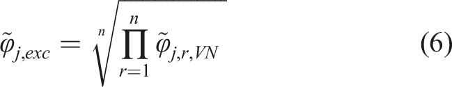
{\tilde{φ}}_{j, e x c} = \sqrt[n]{\prod_{r = 1}^{n} {\tilde{φ}}_{j, r, V N}}

(6)

The result is independent of the number of considered modes and allows comparing groups with different numbers of modes (see also chapter 3.3). To address the risk of double hits, the ADDOFV criterion, equation (3), is used and adapted for the vector normalized eigenvector components, which indicates areas of high velocities, see equation (7). After normalization, a value is calculated, which penalizes points that have high velocities in many of the regarded modes (equation (8))

A D D O F V_{j, V N} = \sum_{r = 1}^{n} \frac{{\tilde{φ}}_{j, r, V N}^{2}}{ω_{r}}

(7)

{\tilde{φ}}_{j, D H} = (1 - (\frac{A D D O F V_{j, V N}}{\max_{j} (A D D O F V_{j, V N})}))

(8)

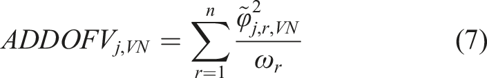
As both values, ${\tilde{φ}}_{j, e x c}$ and ${\tilde{φ}}_{j, D H}$ are normalized to a value between zero and one, their multiplication yields the DPC considering the surface normals, different numbers of modes in a mode group, and the risk for double hits. High values of the DPC indicate good driving points, and by visually representing these values on the surface of the FE-model, an appropriate set of driving points can be chosen.

To illustrate and verify the proposed method, a simple simulation model is used, see Figure 2 left. The model consists of two plates that are meshed in different element sizes and are connected to each other by a fixed connection. On the right of Figure 2, the mode shapes of the first three eigenmodes of the model in free–free condition are shown.

Figure 2.

Left: the FE-model for verification of the proposed method; right: the first three eigenmodes.

The conventional ODP (equation (1)) considering these three modes is shown in Figure 3 on the left-hand side. All potential driving points are on the corners of the plates as the displacement of all three modes is maximal at these points. The deformation shown in Figure 3 on the left-hand side is an overlay of all three mode shapes considered. However, these points on the corners are not suitable for excitation, as they do not allow for a reproducible excitation. Additionally, the points with high ODP values are also the points with the highest velocities and thus are prone to double hits. The model shows that both the projection to the normal of the surface and the penalty of high-velocity points are required to improve the driving point selection.

Figure 3.

Results for the state-of-the-art method on the simple model for the first three modes. Left: ODP; right: ADDOFV. Note: ODP: optimum driving point; ADDOFV: average driving DOF velocity.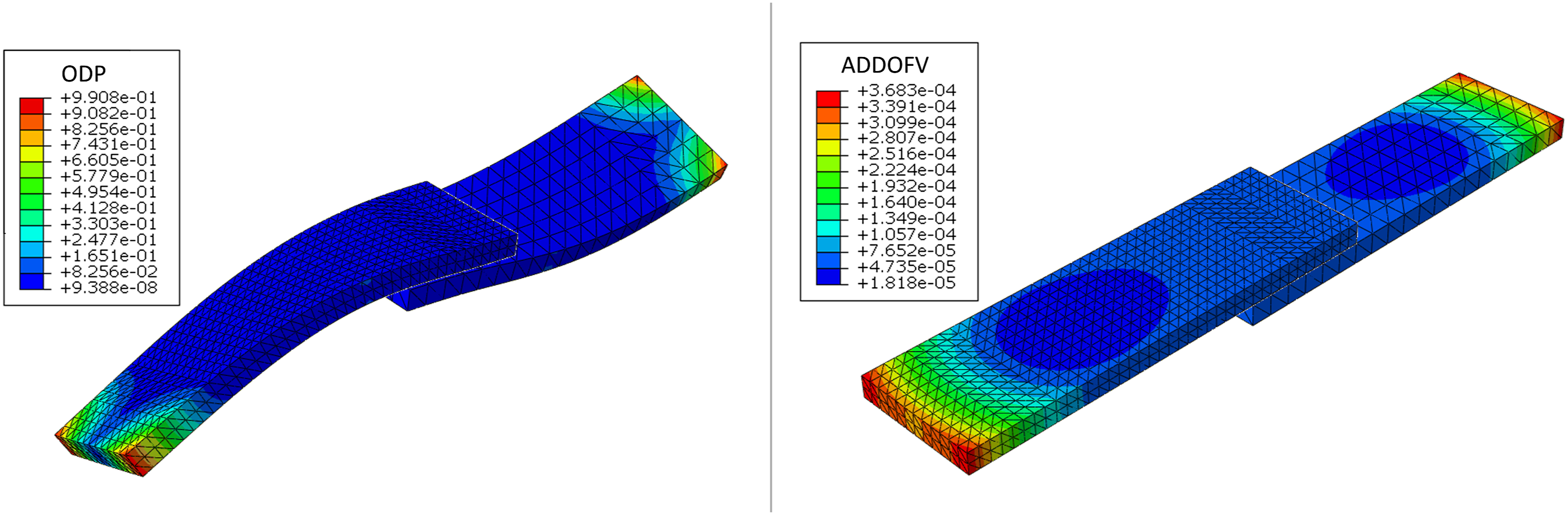

The criteria which are necessary to calculate the DPC are shown in Figure 4.

Figure 4.

Criteria for driving point selection on the simple model for the first three modes. Top left: ODP values for eigenvector components in normal direction; top right: ADDOFV in normal direction; lower left: the product root excitation criterion; lower right: DPC. Note: ADDOFV: average driving DOF velocity; DPC: driving point criterion.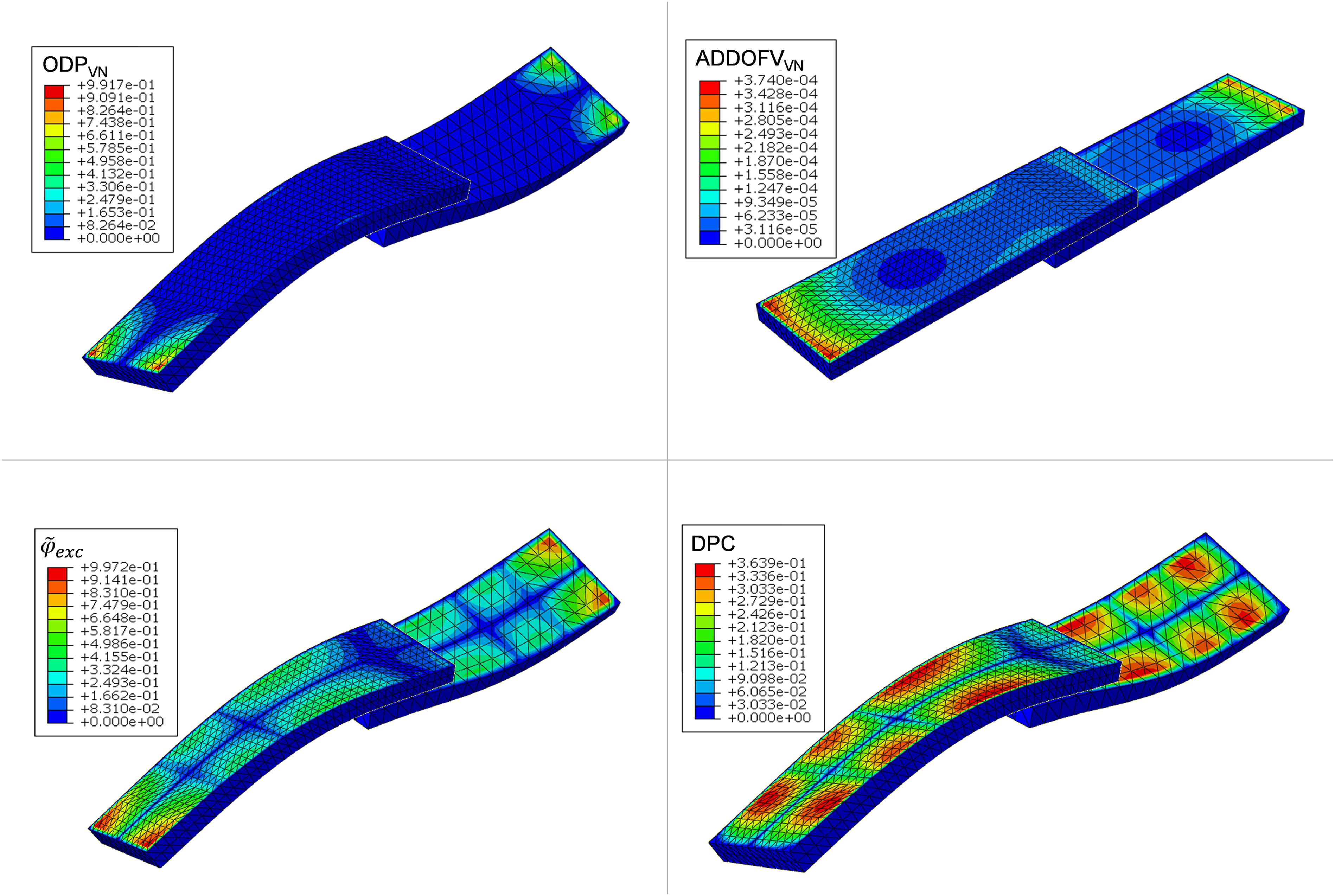

In the top left corner of Figure 4, the influence of the projection to the surface normals is shown by conducting the ODP calculation according to equation (1) with the vector normalized components according to equation (4) $(O D P_{V N})$ . As corners and sharp edges are neither excitable nor do they have a defined normal vector, they are excluded from the calculation. In comparison to Figure 3, the points on the smaller faces of the plate’s model are not considered for excitation anymore, as a tangential excitation would be necessary. However, without the additional modifications, the driving points would still be prone to double hits because of high ADDOFV values shown in the top right corner of Figure 4 – again, only the normal velocities according to equation (7) are considered. When comparing the two diagrams on the left-hand side of Figure 4, the influence of the product root (see equation (6)) can be seen. While the highest values stay close to one, other points appear with values between about 0.2 and 0.6 that might only have a DPC for the individual mode of about 0.5. They are completely eliminated from the conventional ODP calculation because of the cubic multiplication for three modes. The DPC presented in the lower right corner of Figure 4 shows several points at lower velocity amplitudes that are suitable for an excitation. The DPC combines the aspects of excitability, double hit avoidance, direction dependency as well as the number of considered modes in the form of a comparable single-number value for the excitation quality for each DOF and any mode combination.

3.3. Automated selection method

For complex structures, it is often not possible to find one single driving point where all modes can be excited. To identify as little driving points as possible nonetheless, driving points exciting several modes must be found which leads to the creation of groups of modes, which are each excited by one driving point. Identifying suitable driving points thus shifts from trying to identify the best point for all modes to finding the minimum amount of driving points which will sufficiently excite all modes of the system.

The corresponding method proposed as part of this work is depicted in Figure 5.

Figure 5.

Method for enhanced optimum driving point determination.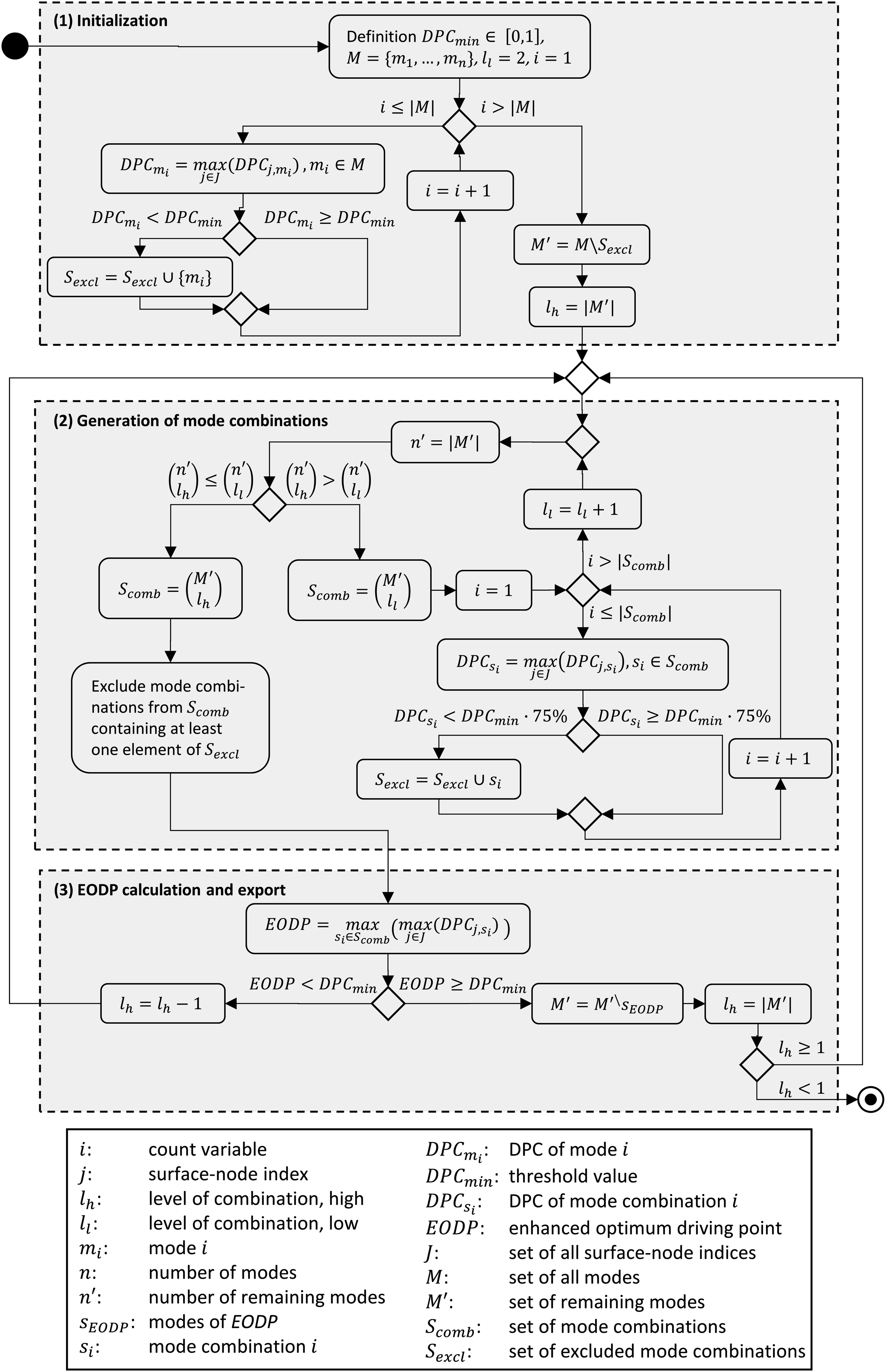

The input parameters to this method are the normalized projected eigenvector components for every mode $m_{i}$ in the mode set $M$ , the calculated vector normalized ADDOFVs for every node, and a user-defined threshold value $D P C_{min}$ for the indicator criterion. Threshold values of 0.2–0.35 have proven to be suitable across applications as a compromise between excitability and avoidance of double hits.

In the beginning, modes with an individual DPC smaller than the threshold value are excluded from the calculation and written into the set of excluded mode combinations $S_{e x c l}$ . The corresponding algorithm is described in part (1) “Initialization” of Figure 5. For the remaining mode set $M ’$ , the “Generation of mode combinations” (part (2)) is conducted. Initially, the higher combination level $l_{h}$ is set to include all modes, while a lower combination level $l_{l}$ is defined as to include all pairs of two modes. The set of combinations $S_{c o m b}$ is created for a subset of $l_{h}$ , or respectively $l_{l}$ , distinct elements of $M ’$ . The number of elements in the set $S_{c o m b}$ is calculated by the binominal coefficient with the number of modes $n'$ choosen $l_{h}$ , or respectively $l_{l}$ . On the basis of the computational efficiency defined by the binomial coefficients, two options are possible: Either, the DPC is evaluated for all mode combinations in the corresponding higher level of combination, depicted in part (3) “EODP calculation and export,” or ill-matching modes are excluded on the lower combination level, shown on the right-hand side of part (2). The algorithm always starts at the higher combination level and calculates the DPC values for each mode group. If mode combinations have been excluded on the lower combination level, all mode combinations in the corresponding higher combination level including these groups are not considered to increase computational efficiency, as these combinations are unlikely to yield good results. The highest DPC value of all mode combinations is picked as the EODP value. If this value is below the threshold, the higher combination level will be reduced and the calculation will be restarted. If, however, the EODP value is larger than the threshold, the corresponding modes will be excluded from further calculation, as a suitable mode combination has been found. If modes are left which are not included in the EODP-combination, the calculation will restart accordingly with the remaining modes.

The second path in part (2) excludes ill-matching mode combinations from the combination calculation in order to minimize the calculation effort. This is done if the calculation of the lower combination level is faster than the one for the higher combination level. In this case, DPC values for all mode combinations of the corresponding lower combination levels are calculated and compared to a value 75% of the threshold value. If a mode combination is lower than this value, it will not be included in further combination calculations. 75% has been found to be suitable across applications and represents a tuning parameter for the engineer to weigh up calculation quality against calculation efficiency. The smaller the value, the lower is the increase of the computation efficiency. However, with a value of 100%, promising mode combinations are eventually ignored, since the values of $D P C_{S_{i}}$ of different mode combinations could compensate each other.

To demonstrate the presented automated selection method, the model presented in Figure 2 is used, considering 20 modes. The driving point indicator for all modes is 0.186 which is less than the defined threshold value of 0.3. Therefore, the modes are grouped into two groups which can be excited at the points marked in Figure 6. By the combined deformation of all the modes excited in the respective mode groups, it is clearly visible why two groups are necessary: The modes of the two plates act in two different planes which cannot be excited by one driving point.

Figure 6.

Result of enhanced optimum driving point calculation with threshold of 0.3 for 20 modes divided into two groups.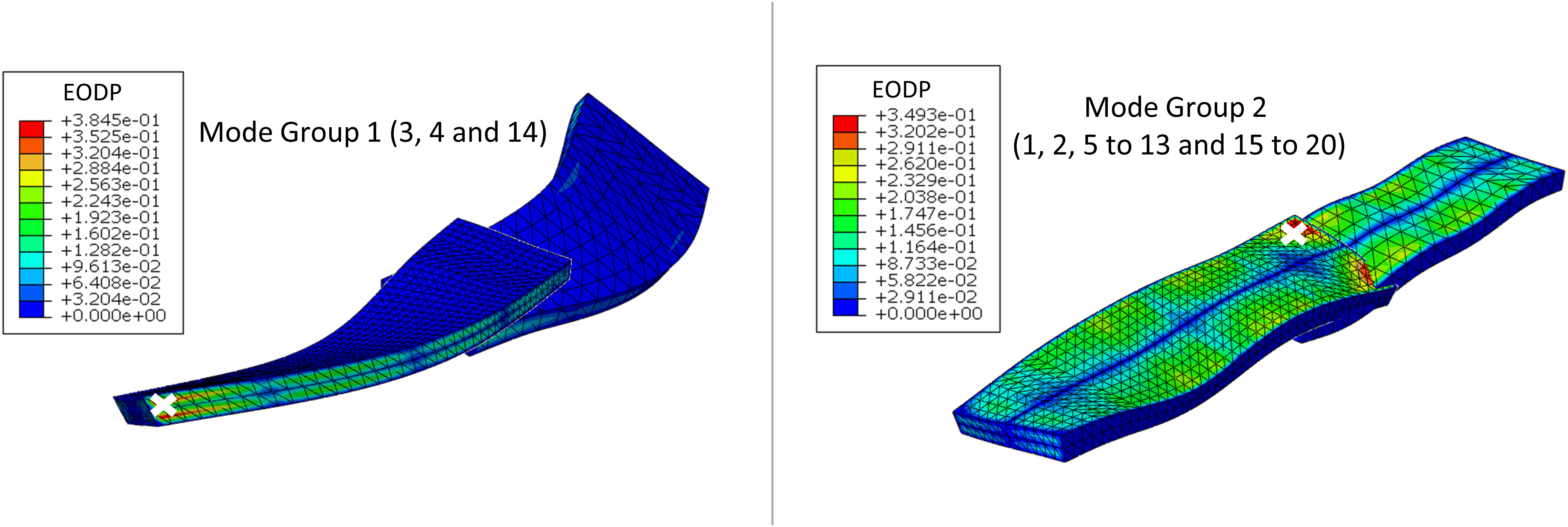

4. Validation

The developed EODP method is demonstrated on two practical application examples. The ODP according to equation (1) is calculated as a reference to the state-of-the-art method. The DOFs with the highest ODP respective EODP values are selected as driving points. The first application example is an aluminum beam structure with a high risk of double hits at many regions. The second application example is a gearbox housing of a tractor, which exhibits a high mode density and large surface area and thus many possible driving points.

Using NMA, the ODP and the EODP values are determined for all modes of the frequency range of interest. The deduced driving points are used for experimental modal testing. The structures are supported in free–free condition and excited at the calculated driving points with a modal hammer. The structure response is measured directly beside the driving point with an acceleration sensor in normal direction. By dividing the measured acceleration by the measured force, the frequency dependent FRF, the so-called driving point FRF, is calculated. Peaks in the FRF are indicating excited modes. The excited modes are automatically identified by using the complex mode indicator function, implemented in the analysis software ME’ScopeVES (Vibrant Technology, 2021). Subsequently, a comparison of the proposed and actually excited modes is made.

4.1. Academic beam

The first application is an aluminum beam, originally designed to study joint damping (Brake, 2018), depicted in Figure 7 on the left. As it is a light-weight structure, high surface velocities occur during impact measurements, thus posing a risk for double hits. Therefore, the proposed method has been applied to this example, to validate if the method allows for the identification of points less prone to double hits. A frequency range of 5 kHz has been chosen to include a total of eight modes in the relevant frequency range. Two groups of modes are necessary to account for the bending modes in both planes. Figure 7, the right one, shows the identified driving points according to the conventional ODP and the proposed EODP method. The coloring of the beam model corresponds to the combined deformation of the first EODP mode group.

Figure 7.

Left: configuration for experimental measurement; right: results of ODP and EODP calculation with the combined deformation of the modes of the first EODP mode group. Note: ODP: optimum driving point; EODP: enhanced optimum driving point.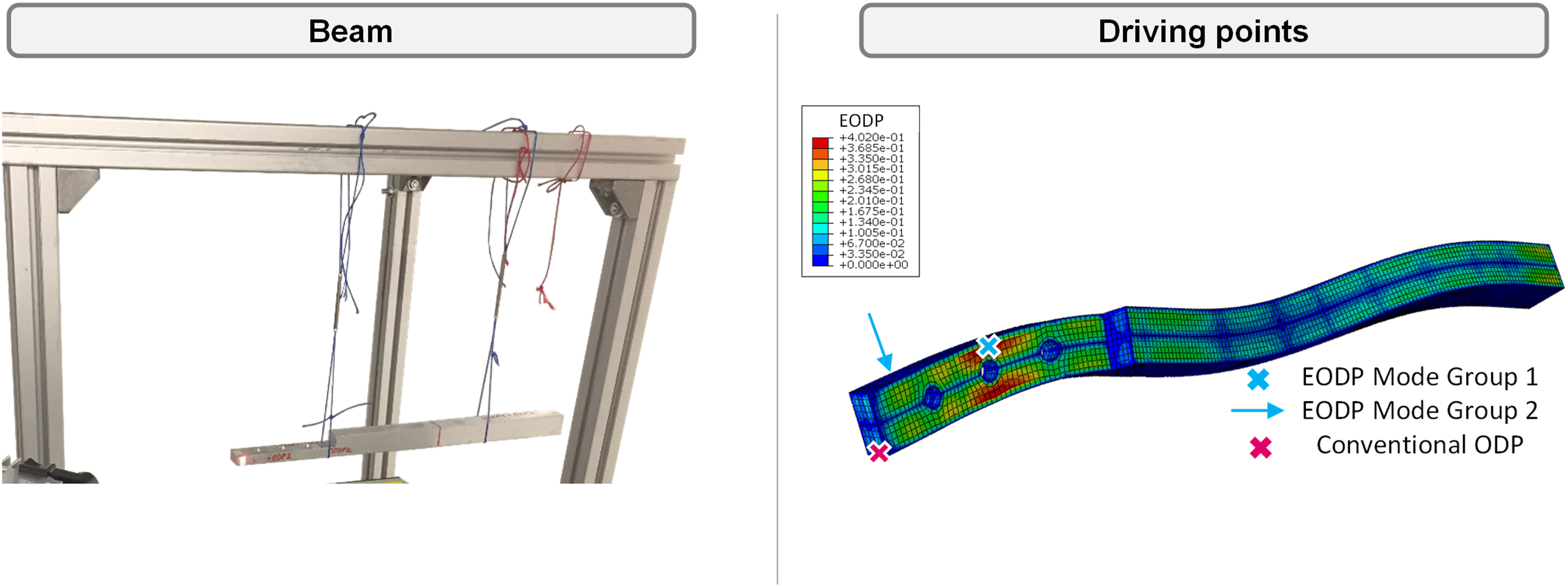

Impact measurements have been carried out in which ODP and EODP have been used for excitation. Several impacts have been conducted at both driving points for both mode groups. It was not possible to avoid double hits at the conventional ODP whereas it was easily possible at the EODP. The calculated and from the measured FRFs identified modes are compared in Figure 8, showing that the EOPD still excites all the modes in the corresponding mode groups.

Figure 8.

Excited modes with the enhanced optimum driving point calculation of the beam.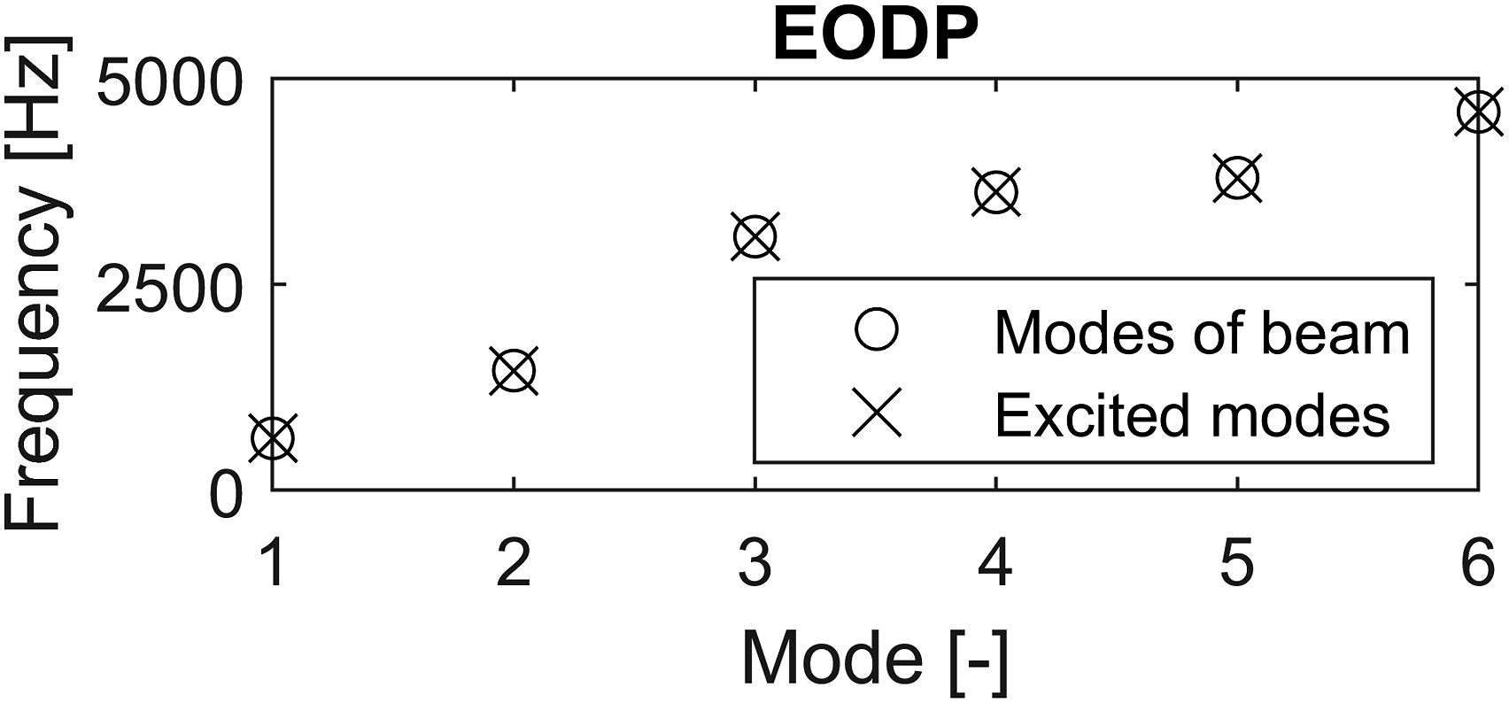

In conclusion, the application shows that the proposed method is able to identify driving points with a low risk for double hits even on critical components, such as light-weight parts. It therefore enables the test engineer to carry out EMAs faster and more reliable.

4.2. Tractor gearbox housing

The second application example is a gearbox housing of a tractor, also presented in Pasch et al. (2020). It aims at demonstrating the use of the presented method on complex examples. The assembly consists of nine separate parts, which are connected by screw connections, see Figure 9. The assembly has a complex geometry with many freeform surfaces and high wall thicknesses which renders double hits improbable.

Figure 9.

Gearbox housing of a tractor.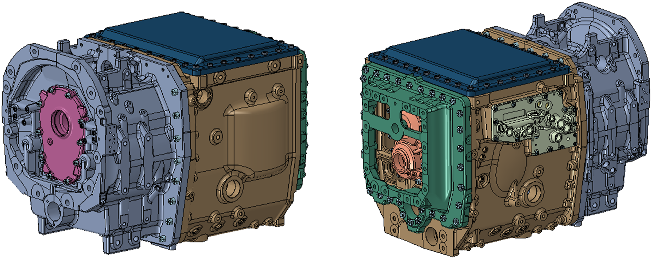

There are 22 modes in the frequency range of interest up to 1 kHz. Due to the high number of modes and high differences in the mode shapes, it is hardly possible to predict suitable driving points without a calculation method. The FE-model of the housing used in this study contains about one million surface DOFs each representing a possible driving point considered in the calculation.

The ODP according to equation (1) is shown in Figure 10, left. The calculation time of the ODP was 1.9 h. The highest value is found in the middle of the gearbox cover. In order to compare both methods, the highest (E)ODP values are selected as the driving point without additional interpretations according to a robust indicator for an automated selection method. Subsequently, the driving point FRF is determined on the real housing. The measurement setup is shown in Figure 10, right.

Figure 10.

Left: ODP for 22 modes, right: experimental measurement setup of the driving point FRF at the ODP. Note: ODP: optimum driving point; FRF: frequency response function.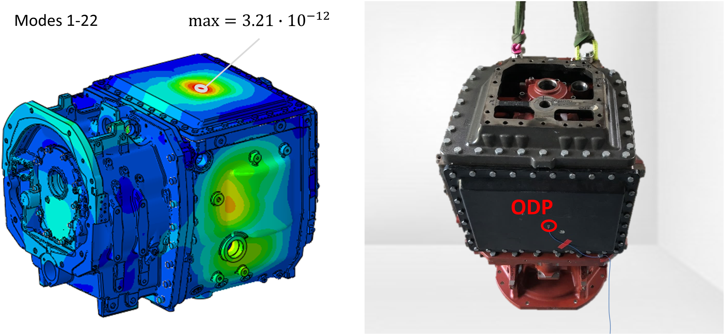

No double hits occurred when exciting the structure. The modes excited at the ODP were determined from the measured data and are shown in Figure 11.

Figure 11.

Excited modes with optimum driving point calculation for the gearbox housing.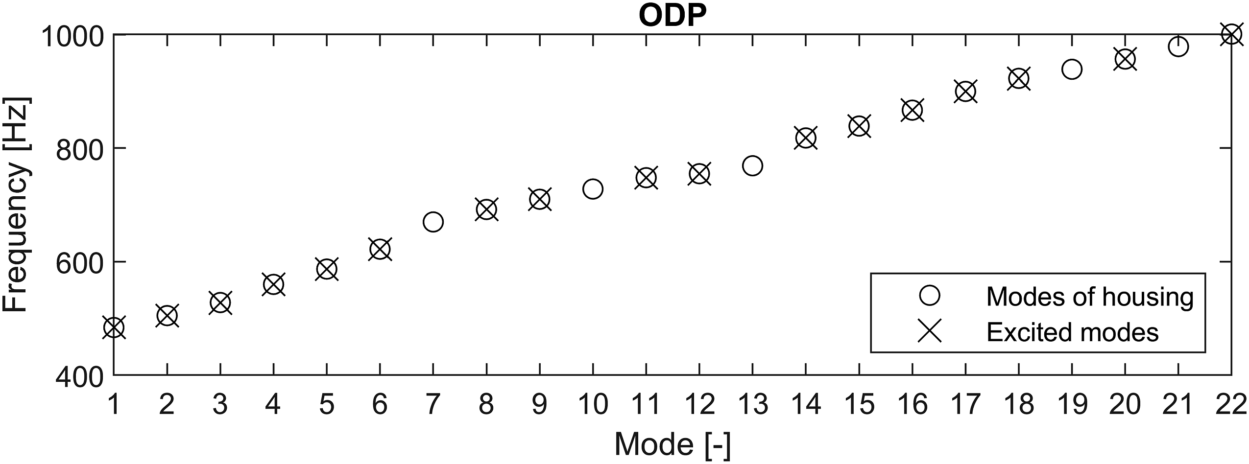

The diagram shows that only 17 out of the 22 modes of the relevant frequency range were excited. Five modes, mode 7, 10, 13, 19, and 21, were not excited at the calculated ODP. Therefore, using the calculated ODP as the driving point, a full EMA, and a full validation of a numerical model could not be performed.

Second, the EODP is calculated as presented in chapter 3.3. The threshold $D P C_{min}$ was set to 0.2. A minimum number of two driving points was determined for the selected threshold, Figure 12. The total calculation time was 3.7 h.

Figure 12.

Enhanced optimum driving point for 22 modes with a threshold of 0.2.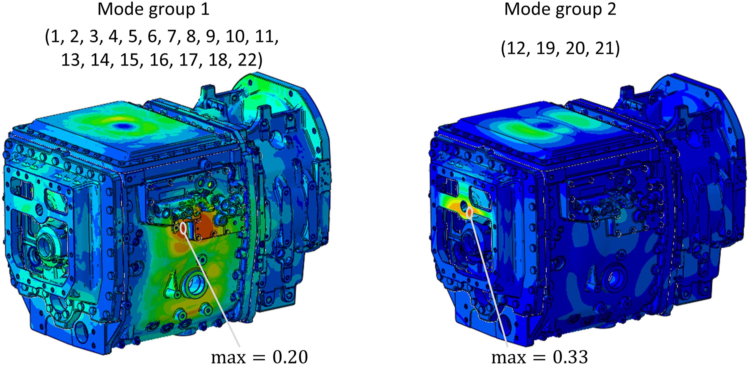

In the experimental test, no double hits occurred at the driving points. Using the two measured driving point FRFs, the excited modes were determined, see Figure 13.

Figure 13.

Excited modes with enhanced optimum driving point calculation for the gearbox housing.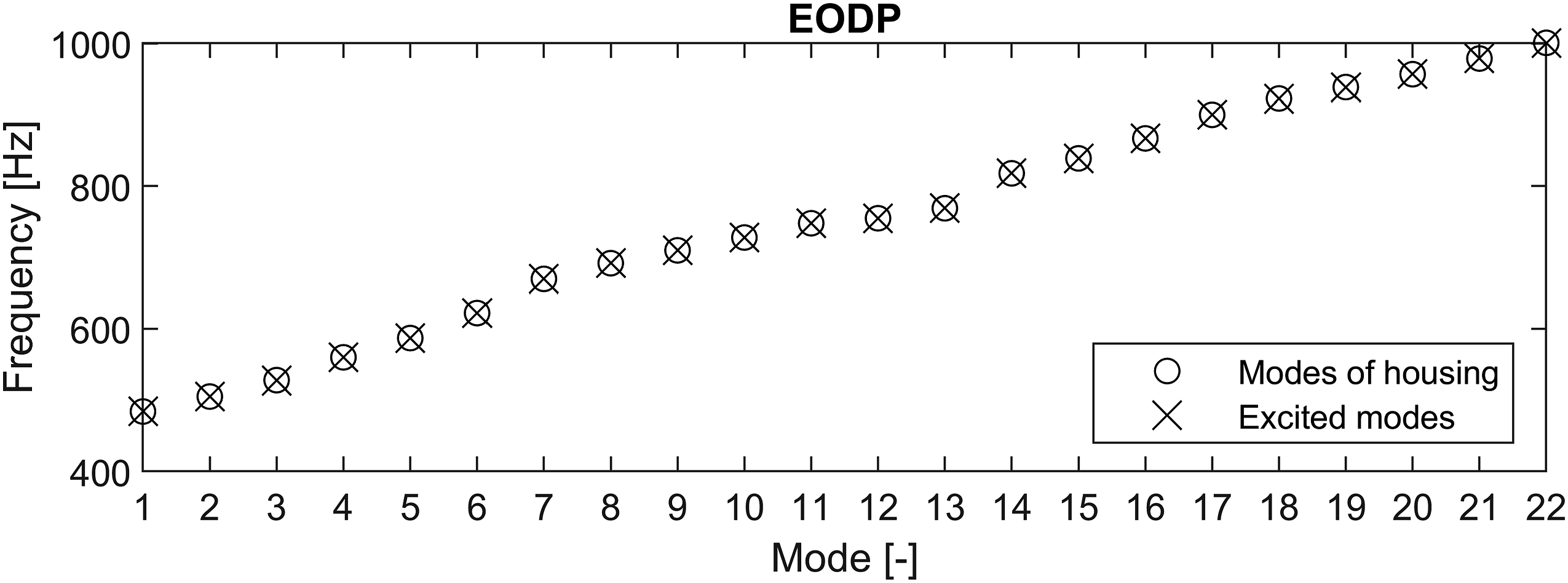

The results show that all 22 modes of the considered frequency range are excited with the predicted set of driving points. Therefore, the points are suitable for performing an EMA.

4.3. Discussion

The application examples underline that the state-of-the-art method is insufficient for the automated calculation of driving points. The academic beam shows the relevance of considering excitability and double hit prevention simultaneously. The tractor housing demonstrates that one single driving point is often not sufficient for practical structures with many modes.

Using the method proposed in this paper, driving points have been successfully predicted for both application examples. For both examples, all modes of the frequency range of interest were excited while no double hits occurred at the selected points during the measurement. Theoretically, there are more than four million $(2^{22} - 1 = 4,194,303)$ possible mode combinations for the 22 modes of the tractor housing. Out of the approximately four million combinations and one million possible surface DOFs, a set of two suitable driving points was determined within less than 4 h. The computation time is small in relation to the time for preparation, execution, and analysis of the measurement. Compared to the state-of-the-art methods, the EODP method offers significant potential for time savings by avoiding iterations and manual evaluations for the selection of driving points.

5. Conclusion and outlook

This paper presents a new method for driving point determination for practical modal testing. For this purpose, an evaluation criterion was presented to determine the excitation quality of possible driving points and possible mode combinations: the Driving Point Criterion (DPC). In the form of a comparable single-number value, this criterion considers the excitability of modes, the avoidance of double hits, the possible excitation direction, and the number of considered modes simultaneously. On the basis of the DPC, an efficient automated selection method is presented, which determines the optimum set of driving points. The result of the selection method are mode groups with a respective driving point location, the enhanced optimum driving point (EODP).

The method was implemented and applied for two different practical application examples. The validation with experimental modal hammer measurements demonstrates the practical use of the method. For both examples, all modes of the frequency range of interest were excited using the EODP, whereby double hits were avoided.

In further work, automated methods for determining the minimum necessary response positions and the optimal suspension positions for modal testing of complex structures are to be developed by using the indicator values presented.

Footnotes

Declaration of conflicting interests

The author(s) declared no potential conflicts of interest with respect to the research, authorship, and/or publication of this article.

Funding

The author(s) received no financial support for the research, authorship, and/or publication of this article.

ORCID iDs

Gerwin Pasch

Stefan Wischmann

Georg Jacobs

References

Allemang

Brown

(1982) A correlation coefficient for modal vector analysis. In: Proceedings, 1st International Modal Analysis Conference, Orlando, Florida Ewins, 8–10 November 1982, pp. 110–116.

Brake

(2018) The Mechanics of Jointed Structures: Recent Research and Open Challenges for Developing Predictive Models for Structural Dynamics. Cham: Springer International Publishing.

Brandt

(2011) Noise and Vibration Analysis: Signal Analysis and Experimental Procedures. Chichester, UK: John Wiley and Sons Ltd.

Donaldson

Mechefske

(2020) Experimental modal analysis of business jet fuselage tail section sub-assemblies. In: Volume 7: 32nd Conference on Mechanical Vibration and Noise (VIB), Virtual, Online, 17–19 August 2020. American Society of Mechanical Engineers.

Døssing

(1988) Structural Testing: Part 1, Mechanical Mobility Measurements. Brüel & Kjær Primer.

Ewins

(2000) Modal Testing: Theory, Practice and Application. Baldock: Research Studies Press.

Imamovic

(1998) Validation of Large Structural Dynamics Models Using Modal Test Data. Dissertation, University of London, London.

Imamovic

Ewins

(1997) Optimization of excitation DOF selection for modal tests. Proceedings of SPIE, the International Society for Optical Engineering 3089: 1945–1951.

Koksal

Yildiz

Yazicioglu

, et al. (2014) Ground vibration test planning of a fighter aircraft by using a rough finite element model. In: Proceedings of the ASME International Mechanical Engineering Congress and Exposition - 2013, San Diego, California, USA, 15–21 November 2013. New York, NY: ASME.

10.

Law

Phani

Altintas

(2013) Position-dependent multibody dynamic modeling of machine tools based on improved reduced order models. Journal of Manufacturing Science and Engineering 135(2): 021008.

11.

Liu

Qiu

Zhao

Cui

(2020) Modal Analysis and Experimental Study of Marine Gear Box. Journal of Physics: Conference Series 1549: 032119.

12.

Mali

Singru

(2018) Study on the effect of the impact location and the type of hammer tip on the Frequency Response Function (FRF) in experimental modal analysis of rectangular plates. IOP Conference Series: Materials Science and Engineering 330: 12102.

13.

Nåvik

Derosa

Rønnquist

(2021) On the use of experimental modal analysis for system identification of a railway pantograph. International Journal of Rail Transportation 9(2): 132–143.

14.

Oktav

(2020) Identification of non-proportional structural damping using experimental modal analysis data. Journal of Measurements in Engineering 8(1): 34–45.

15.

Oza

Shah

(2020) Theoretical and experimental modal analysis of centrifugal pump radial flow impeller. IOP Conference Series: Materials Science and Engineering 992: 012003.

16.

Pasch

Jacobs

Berroth

(2020) NVH system simulation of a tractor with hydrostatic-mechanical power split transmission. Landtechnik 75(4): 301–315.

17.

Pedramasl

Şahin

Acar

(2017) Enhancement of quality of modal test results of an unmanned aerial vehicle wing by implementing a multi-objective genetic algorithm optimization. Aerospace Science and Technology 71: 447–463.

18.

Siemens (2020) Simcenter 3D Pre/Post overview: Simcenter 3D 2020.2 Series. Available at: https://docs.sw.siemens.com/en-US/product/289054037/doc/PL20191127135404299.advanced/html/id626011.

19.

Vibrant Technology I (2021) MEscope VES-4000 Modal Analysis: Manuals. Available at: http://manuals.vibetech.com/10.ModalAnalysis.pdf (accessed 26 March 2021).

20.

Wegerhoff

(2017) Methodik zur numerischen NVH Analyse eines elektrifizierten PKW Antriebsstrangs. Dissertation, RWTH Aachen, Aachen.

21.

Ziaei Rad

(2005) Finite element, modal testing and modal analysis of a radial flow impeller. Iranian Journal of Science and Technology, Transaction B: Engineering 29(2): 157–169.

Enhanced method for optimum driving point identification for modal testing