
Abstract
Studying emotion dynamics through time series models is becoming increasingly popular in the social sciences. Across individuals, dynamics can be rather heterogeneous. To enable comparisons and generalizations of dynamics across groups of individuals, one needs sophisticated tools that express the essential similarities and differences. A way to proceed is to identify subgroups of people who are characterized by qualitatively similar emotion dynamics through dynamic clustering. So far, these methods assume equal generating processes for individuals per cluster. To avoid this overly restrictive assumption, we outline a probabilistic clustering approach based on a mixture model that clusters on individuals’ vector autoregressive coefficients. We evaluate the performance of the method and compare it with a nonprobabilistic method in a simulation study. The usefulness of the methods is illustrated using 366 ecological momentary assessment time series with external measures of depression and anxiety.
Keywords
In recent years, psychology has profited increasingly from the inclusion of temporal dynamics into its theories and assessment, for instance, with regard to the development of emotions and psychopathology over time and across places (Bos, Schoevers, & aan het Rot, 2015; Hamaker, Grasman, & Kamphuis, 2016; Jebb, Tay, Wang, & Huang, 2015; Koval, Kuppens, Allen, & Sheeber, 2012). This development and the emergence of ambulatory assessment (AA) techniques have propelled a focus on ideographic models. These models center on the dynamics of a single individual to fully express individual characteristics (Molenaar, 2004). This provides rich insight into the dynamic variation within an individual. The ideographic approach contrasts to the traditional, nomothetic approach, where general predictions about the population are derived based on the variation between individuals. Despite their popularity ideographic approaches also have disadvantages, especially being ineffective when studying large samples and lacking generalizability. Fitting a new model for every individual is unwieldy in a large sample. Furthermore, ideographic models often describe the dynamics of a single individual in great detail, but results cannot be generalized to other individuals. This is a severe limitation because psychological researchers typically strive to generalize or at least to assess how an individual compares with others, as is done with nomothetic approaches.
To introduce ideographic approaches for psychological assessment practices, notions of reliability and validity have to be considered. Reliability and validity have been firmly established for nomothetic methods but their application to idiographic methods received comparatively little consideration. Bridging ideographic and nomothetic approaches may enable the derivation of reliable, valid, and standardized assessment methods through normative and generalizable statistical models (Beltz, Wright, Sprague, & Molenaar, 2016; Wright & Zimmermann, 2019). For instance, the interpretation of intraindividual dynamics might be facilitated by standardized tools and comparisons with normative group data. Thus, the recent shift toward ideographic methods propels the need for integrative efforts of the intraperson and interperson perspectives.
To generalize dynamic processes researchers must draw inferences across levels of analysis, such as from the within-person level to the between-person level and vice versa. Often researchers assume that the between-person and within-person processes are equal, which would imply that studying the process at one level suffices to generalize to the other level. This so-called ergodicity assumption fails to hold for most psychological processes, meaning the analysis at one level will yield different results than the analysis at another level (Molenaar, 2004). Some researchers presume that ergodicity would be strictly required to generalize across levels and, in the ubiquitous presence of nonergodicity for psychological processes, abandon generalizations altogether. This is a misconception (Adolf & Fried, 2019), because generalizing within-person dynamics to the between-person level is possible if one can achieve conditional ergodicity (Molenaar, 2004). Conditional ergodicity is met if within-person and between-person structures are equivalent after controlling for the unique factors of both structures, such as autoregression, time trends, or the existence of distinct subgroups (Voelkle, Brose, Schmiedek, & Lindenberger, 2014).
Similar to the concept of ergodicity, researchers investigating the items of multiple individuals over time would like to achieve measurement invariance (MI) across levels, with an absence of measurement differences (also called item bias) across individuals and time. Consequently, MI is a less restrictive condition than ergodicity. It requires only the measurement process to be equivalent and allows for heterogeneity with respect to the latent variables and their interrelations over individuals and time. The threat of unexplained heterogeneity, however, applies similarly to MI as it does to ergodicity; in a heterogeneous sample the intraperson and interperson differences may be too pronounced to achieve MI between levels (Adolf, Schuurman, Borkenau, Borsboom, & Dolan, 2014).
The quest into conditional inferences across levels of analysis requires researchers to identify the sources of heterogeneity at both levels of analysis. A possible reason for nonequivalence between levels could be the existence of subgroups at the between-individual level (Voelkle et al., 2014). Often empirical findings and the provided theoretical underpinnings thereof suggest the existence of subgroups of individuals that exhibit quantitative similarities in their dynamics. These subgroups are assumed to be characterized by individuals that resemble one another in their dynamism, while the subgroups mutually differ in their dynamics. It has been theorized, for example, that different age groups exhibit distinct affective responses to stress (Scott, Sliwinski, & Fields, 2013). Similarly, the dynamic relationships between somatic symptoms and positive and negative affect have been shown to differ in magnitude as well as in direction across individuals (Schenk, Bos, Slaets, de Jonge, & Rosmalen, 2017). For instance, the mutual dynamic relationships of positive and negative affect has been found to differ markedly between patients with Parkinson’s disease (Shifren, Hooker, Wood, & Nesselroade, 1997). Shifren et al. (1997) note, “Thus, despite selecting a sample that was homogeneous with regard to disease type, functional abilities, and cognitive impairment, the results show heterogeneity for the structure and variation of mood.” (p. 336). Such findings suggest that differences in emotion dynamics cannot simply be accounted for by static covariates.
Some statistical approaches that bridge the ideographic and nomothetic approaches, like multilevel analysis, assume similar patterns of effects across the whole sample. While ideographic models circumvent the problem by allowing for heterogeneity in the structures of the models, this property often leads to overfitting. For example, Van der Krieke et al. (2017) used multilevel analysis and ideographic time series models to describe within-person and between-person variability. Results revealed large differences in dynamics between individuals. Neither of the two approaches was able to integrate information of individual dynamics with information on similar dynamics from other individuals, and to give an indication of why individuals’ dynamics differed markedly.
Another approach to bridge ideographic and nomothetic perspectives uses likelihood ratio tests to assess reasons for nonequivalence between structures in multisubject time series (Voelkle et al., 2014). While this procedure allows to test whether equivalence holds across possible sources of heterogeneity, the researcher has to specify the sources of variance a priori. In many cases, the factors that cause nonequivalence between structures are not known. The quest to bridge ideographic and nomothetic approaches has thus motivated the search for meaningful subgroups to stratify the heterogeneous sample into homogenous subgroups.
To assess the dimensions of within-person and between-person differences, we propose an exploratory procedure that identifies subgroups of individuals who differ qualitatively in their within-individual dynamics: a dynamic clustering method. Clustering provides insight into the systematic patterns that cause nonequivalence and allows to draw inferences about both, commonalities and differences of the two levels. Identifying clusters in time series can enable us to distil the signature dynamics of different psychological processes from intensive longitudinal data. This will allow a more precise description of individual developments. Specifically, we propose a clustering method based on the most frequently employed time series model in the social sciences, the multivariate vector autoregressive (VAR) model of order p (cf. Lütkepohl, 2005). VAR parameters enable the description of multivariate dynamic relations in a format familiar to researchers in the field. In contrast to time series clustering procedures proposed so far, we will allow for within-cluster variation by employing a Gaussian finite mixture model to cluster individuals’ VAR coefficients, thereby arriving at a probabilistic clustering.
We investigate the properties of our probabilistic clustering model in a simulation study and illustrate its application on an empirical example; the method’s performance is contrasted to a nonprobabilistic alternating least squares VAR(1) model (Bulteel, Tuerlinckx, Brose, & Ceulemans, 2016). R code for estimating the clustering methods is provided on the projects OSF page at (https://osf.io/sv2tg/?view_only=d57284da4e5f413c8727e6f98a4291fa). Before we outline our dynamic clustering model, we begin with a short overview of clustering methods for longitudinal data.
Clustering Methods for Time Series Designs
Contemporary clustering methods are most commonly divided into two groups: nonprobabilistic 1 and probabilistic approaches. The former operates by minimization of a criterion, for instance, the sum of squares of distances, resulting in a nonprobabilistic assignment of individuals into clusters. The latter involves a statistical model, such as a mixture model that assumes data to arise from a mixture of distributions where each component corresponds to a cluster (McLachlan & Basford, 1988; McLachlan & Peel, 2004). At the heart of time series clustering methods lays the challenge of accounting for the dependence structure that is characteristic to dynamic data. Time series clustering approaches in other fields focus mainly on classification and use feature-based distance measures or compare the individual time points directly (for an interdisciplinary review, see Liao, 2005). The present study is focused on approaches that account for the temporal dependence through a statistical time series model. These approaches hold most promise for psychological research, because they provide a description of the cluster-wise dynamics in terms of interpretable model parameters which allows for generalizability of results. In these models, each cluster consists of time series described by similar model parameters.
Jacques and Preda (2014) contrast adaptive methods and filtering methods to cluster longitudinal data. Adaptive models combine the two crucial steps—accounting for dependency between time points and forming clusters—in a single estimation step, while filtering methods carry out both steps separately. Below, we review shortly the most prominent model-based time series clustering methods for psychological AA data. A classification of these methods is listed in Table 1.
Overview of Model-Based Time Series Clustering Methods for Psychological Data.
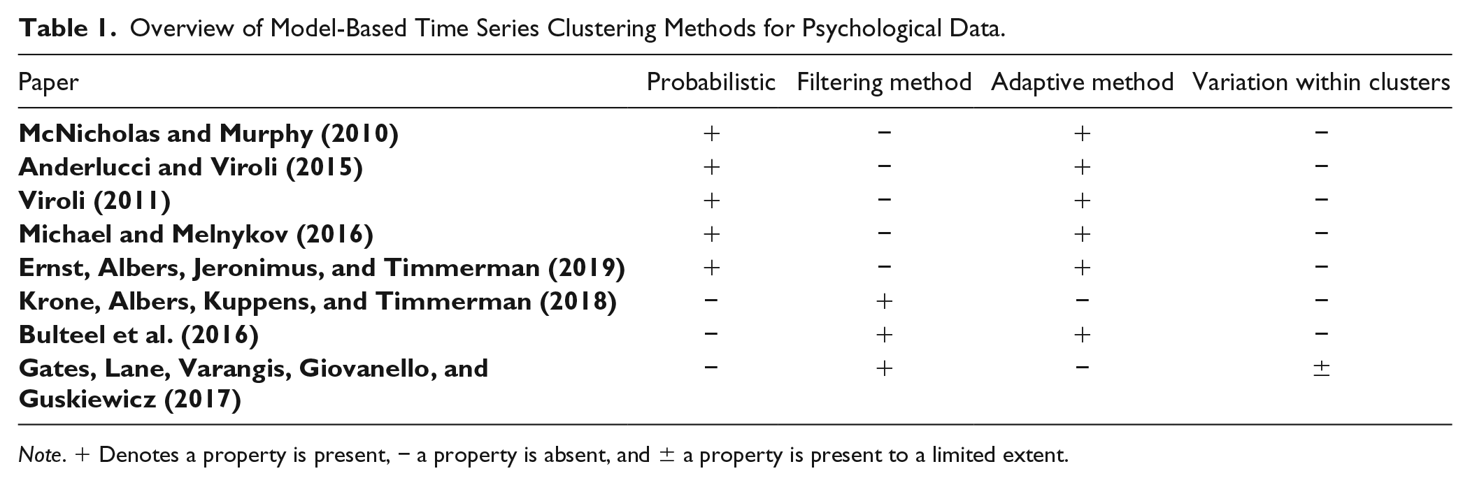
Note. + Denotes a property is present, − a property is absent, and ± a property is present to a limited extent.
Recently, McNicholas and Murphy (2010), Viroli (2011), and Anderlucci and Viroli (2015) proposed probabilistic, adaptive approaches to time series clustering, where each cluster is modelled by an identical generalized autoregressive process. The covariance structure of these models depends on the length of the time series, rendering these models unsuited for time series with a high number of observations and/or unequal length. Recently, probabilistic, adaptive approaches have been proposed for long and unequal time series for the univariate (Michael & Melnykov, 2016) and multivariate case (Ernst et al., 2019).
Adaptive clustering methods offer many advantages over filtering methods. For instance, some are able to describe different clusters through different time series models (for details, see Ernst et al., 2019). These models, however, are very complex and their iterative estimation procedure makes them slow when studying large data sets and scenarios where various numbers of potential clusters and/or potential time series models are considered. As a result, the number of potential models that will have to be compared increases exponentially with the number of time series models and the number of clusters that are considered in model estimation. The use of filtering circumvents scalability problems. Most important, though these adaptive models lack random effects at the individual level. Therefore, these models give no indication of the within-cluster deviation beyond a single white noise error term. So, while elegant holistic models exist to cluster psychological time series, these models assume identical VAR coefficients for individuals of the same cluster. Therefore, the representation does not give indication of the individual deviations from the autoregressive cluster parameters which are highly plausible to exist in psychological AA data.
Bulteel et al. (2016) put a nonprobabilistic, adaptive clustering method forward that clusters multivariate, time series by representing clusters through identical VAR model parameters. That is, the method operates via an alternating least squares method, minimizing the within-group sum of squares based on the VAR parameters of the cluster an individual is assigned to. This results in a nonprobabilistic clustering of individuals. This method does not account for individual variation within clusters.
S-GIMME, a nonprobabilistic, filtering approach, estimates temporal and contemporaneous associations between variables at either the population-, subgroup- (i.e., cluster-), or individual-level (Gates et al., 2017; Lane, Gates, Pike, Beltz, & Wright, 2019). Only effects that significantly improve the modification index at the respective level are estimated. S-GIMME is exceptional in that it accounts for individual differences by estimating individual-level effects. The estimation of associations at various levels distinguishes S-GIMME from the other time series clustering approaches discussed here that estimate the associations between all variables at the cluster-level. While providing a partitioning that takes individual differences into account, S-GIMME provides only limited indication of the within-cluster variation, especially with regard to the associations that are estimated at the population- or subgroup-level.
Krone et al. (2018) used a nonprobabilistic, filtering approach to cluster emotion time series. They employed the autoregressive Bayesian dynamic model as a filter and clustered the resulting parameters with a k-means algorithm.
To relax the rather strict assumption of equal dynamic processes within clusters that has been made (for at least some associations) by the dynamic clustering methods so far, we propose a probabilistic, filtering method. Unlike the methods reviewed above, this will account for and give indication of within-cluster deviation for all estimated dynamic associations.
Proposing a Probabilistic Clustering Procedure Using Finite Mixture Models
The probabilistic clustering method proposed in this article accounts for the variation in both, the individual dynamics and the individual mean levels, by clustering on both VAR slopes and intercepts. The method proceeds in a two-step fashion: (a) summarizing individuals’ multivariate dynamics by use of the VAR(p) model and (b) probabilistic clustering of model parameters of Step 1, based on the Gaussian finite mixture model (McLachlan & Basford, 1988; McLachlan & Peel, 2004).
Summarize Individual Time Series
The VAR model of order p, VAR(p), for an individual j (j = 1, … ,j) is given by the following equation:
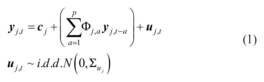
with
For each individual’s time series, the most parsimonious lag order (pj) balanced with goodness of fit can be determined by model selection criteria such as the Bayesian information criterion (BIC; Schwarz, 1978). Based on this, the highest (plausible) lag to capture all the individual process in the sample can be selected (i.e., p = max(pj)). We propose to subsequently estimate a VAR model of lag p for all individuals. 2 Because mixture model approaches to clustering are known to show disappointing performance in high-dimensional space (Bouveyron & Brunet-Saumard, 2014), and to avoid overfitting, overparametrization through an unnecessarily high lag order should be avoided. Similarly, only a moderate number of variables, say between two and seven, should be clustered using the approach proposed here.
Probabilistic Clustering
Once VAR intercepts and slopes are obtained for every individual the distribution of VAR coefficients can be estimated through a finite mixture model. Specifying probability distributions per cluster rather than using fixed values, we relax the assumption of identical parameters for individuals within a cluster as in the method by Bulteel et al. (2016). The probability density function of obtaining

where

The parameters are estimated via maximum likelihood. After
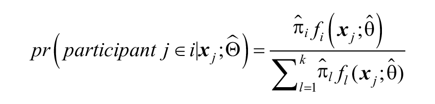
with component densities fi assumed to have the N(µi,
In the context of a finite mixture model, the selection of the number of clusters can be conceived of as a comparison between statistical models, where the different statistical models represent different choices for the number of clusters. Similarly, models with different constraints about the structure of the
Autoregressive Representation of Time Series as Filter
The clustering based on filtered VAR coefficients as we propose here offers the following advantages: (a) Condensing the observed time series into model parameters before clustering reduces the high dimensionality that is characteristic for multivariate time series data. This problem, the curse of dimensionality (Bellman, 1957), can lead to highly biased estimates during the clustering process. VAR coefficients offer a reduction of dimensionality in which meaningful features are extracted from the data by use of the VAR model; (b) Clustering on VAR coefficients allows for comparison of time series of differing length; (c) VAR coefficients enable the description of multivariate dynamic relations in a format familiar to researchers in the field. That is, VAR coefficients represent the dependence structure of a time series, and thus summarize the dynamics of individuals in a meaningful way.
For instance, emotional inertia, the propensity of affective states to resist to change, is often considered a key component of psychological well-being. This temporal dependency gives insight into a crucial and often neglected component of emotional well-being (Koval & Kuppens, 2012). High emotional inertia may be indicative of impaired emotion regulation, as a lack of emotion regulation may result in an inability to recover from negative emotions. It might also be indicative of a heightened preoccupation that results in emotional insensitivity and decreased involvement with the environment (Brose, Schmiedek, Koval, & Kuppens, 2015). Emotional inertia is traditionally operationalized as the autoregressive coefficient of an emotion (Koval et al., 2012; Krone et al., 2018). Because VAR coefficients are multivariate in nature, they provide insight into the dynamics of individual emotions, as well as the dynamics between the various emotions.
Sequential procedures to clustering, as outlined here, can be jeopardized when the reduction technique of the first step selects a summary of the data that is not discriminant of the different groups (Bouveyron & Brunet-Saumard, 2014). Our filtering method can be expected to be appropriate as long as VAR coefficients provide a proper indication of the underlying dynamics. An exception of this condition occurs, for instance, if the processes under study are not time-invariant, but meaningful changes in individuals’ dynamic development occur during the course of the study, for instance, due to an intervention (see, e.g., Bringmann et al., 2017).
Also in other fields has the distance between time series parameters been widely applied as filter in nonprobabilistic clustering algorithms, especially the Euclidean distance between autoregressive coefficients, for instance, in combination with k-means or fuzzy C-medoids (D’Urso, De Giovanni, & Massari, 2015; D’Urso, De Giovanni, Massari, & Di Lallo, 2013). These measures are popular because of the absolute convergence of the autoregressive sequences of processes belonging to the admissible ARIMA (autoregressive integrated moving average) class. Thus, the distance between vectors of autoregressive parameters is a measure of structural dissimilarity between two time series processes. The distance indicates the cluster to which the dynamical structure of a series is closest.
Employing a Gaussian mixture distribution, we assume the individual VAR coefficients to be normally distributed around the mean of their associated cluster. The within-cluster covariance matrix can be freely estimated, which allows flexibility with regard to the orientation and distribution of the different clusters. The distance between maximum likelihood estimates of autoregressive parameters of two time series originating from a processes with the same dynamical structure will be asymptotically multivariate normally distributed for stationary and nonstationary time series of any lag order (Corduas & Piccollo, 2008). Provided that time series within a cluster are generated by an identical dynamical process, VAR coefficients will thus asymptotically distribute normally around their cluster mean. This implies that model misspecification with regard to the number of clusters and/or a small sample size might thus cause the different cluster components to be nonnormally distributed. The Gaussian mixture model, however, has been shown largely robust to deviations (e.g., deviations caused by upper and lower limits or even uniform distribution within clusters (Steinley & Brusco, 2011). Because we assume the existence of clusters that are generated by at least structurally similar dynamic processes, we assume the within-cluster distribution of VAR coefficients will be well-captured by a normal distribution.
In the following, we will investigate the performance of our model-based clustering method in a simulation study and show its usefulness on an empirical ecological momentary assessment data set. The method shall be compared with an adaptive, nonprobabilistic clustering method (Bulteel et al., 2016).
Simulation
Simulation 1: Equal Intercepts Between Clusters
To assess the performance of the proposed probabilistic clustering method, we will conduct the following simulation. The performance of the probabilistic and nonprobabilistic method (Bulteel et al., 2016) will be compared with regard to recovery and optimization. Recovery is evaluated as the degrees to which the cluster membership and the cluster-specific VAR slopes can be retrieved; optimization is determined as sensitivity to local minima. We will investigate to what extent these two performance aspects depend on six data characteristics. Four of these factors pertain to the partition of individuals: (a) the number of clusters, (b) the relative cluster sizes, (c) the distance between clusters, and (d) the variation within clusters. Two factors reflect efficiency: (e) the number of individuals and (f) the number of time points (Tj). Regarding these factors, we have the following hypotheses: the performance of the clustering methods will decrease with (a) a higher number of clusters, (b) larger differences in relative size of the clusters, (c) lower distance between clusters, (d) higher variation within clusters, (e) fewer individuals, and (f) fewer time points. Also, we expect the probabilistic clustering method proposed in this article to outperform the nonprobabilistic clustering method as soon as variation within clusters is introduced, and to show a smaller vulnerability to differences in relative cluster size. All simulation and analysis were carried out in R (R Core Team, 2017). R code for estimating the clustering methods is provided in the supplementary material (available online) and on the projects OSF page at https://osf.io/sv2tg/?view_only=d57284da4e5f413c8727e6f98a4291fa.
Design and Procedure
For every individual, a time series was generated according to Equation (1). Herewith, the following factors were kept constant: the variance–covariance matrix of the white noise series
The number of clusters k: 2 or 4.
The relative size of the clusters: Equal distribution of participants across clusters; minority condition, with one cluster containing 10% of participants and the rest evenly distributed across the remaining clusters; majority condition, with one cluster containing 60% of individuals and the remaining individuals evenly distributed over the other cluster(s). 5
The distance between the different clusters as expressed through distance between VAR(1) regression coefficients matrices of the different clusters. For every cluster in every condition, we simulated a matrix that contained the mean VAR(1) regression coefficients of the cluster. For each variable, all autoregressive and cross-regressive effects were generated with autoregressive coefficients on the diagonal and cross-regressive associations on the off-diagonal. In all conditions, autoregressive weights in the VAR coefficient matrix
The variation between individuals of the same cluster (within-cluster distance): 6
Identical underlying VAR(1) regression coefficients for individuals of the same cluster, where for each individual j in cluster i
The total number of individuals: 30, 60, or 120.
The number of time points per person: 51, 101, or 501.
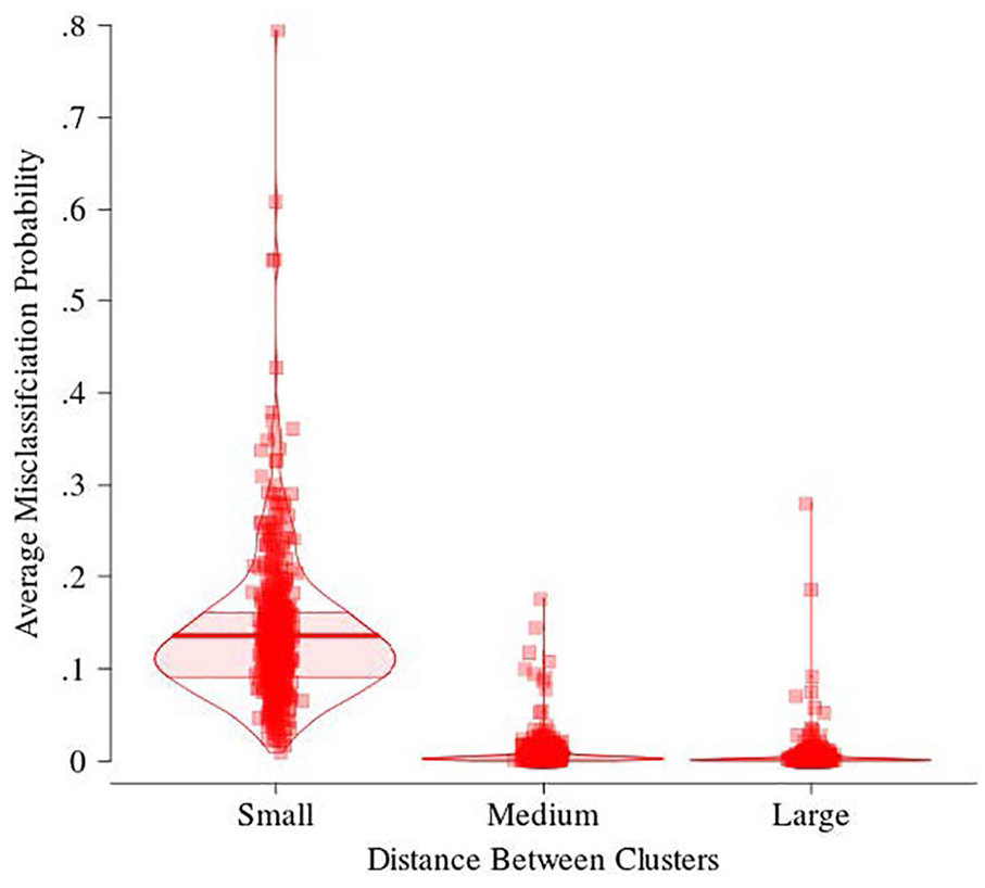
Distribution of average misclassification probability in the similar-true-parameters conditions across the three between-cluster distance conditions.
For each of the resulting 324 conditions, we simulated 10 data sets. Subsequently, a probabilistic and a nonprobabilistic clustering analysis with the true number of clusters and correct lag order of p = 1 was performed on each data set with 1 rational start and 100 random starts. The nonprobabilistic clustering method had a rational initialization where the VAR(1) regression slopes were partitioned by use of hierarchical agglomerative clustering via Ward’s criterion (Ward, 1963). The rational initialization of the EM algorithm used a partition reached by model-based hierarchical agglomerative clustering of individuals’ regression slopes and intercepts. This method begins with clusters containing one individual each and merges the two clusters that are associated with the lowest decrease in classification likelihood for the mixture model (Banfield & Raftery, 1993).
The nonprobabilistic clustering method was estimated through an alternating least squares approach as proposed by Bulteel et al. (2016), using R. The code for estimating the method is provided in the supplementary material available online. The probabilistic clustering method was estimated by first determining VAR(1) coefficients using least squares estimation, subsequently clustering was carried out by use of the EM algorithm (Dempster et al., 1977) included in the mclust R package (version 5.3, Fraley & Raftery, 2002; Fraley, Raftery, Murphy, & Scrucca, 2012). The cluster parameters,
Simulation 2: Unequal Intercepts Between Clusters
To evaluate how much the performance would improve for between-cluster differences in intercepts, we conducted a second simulation. This simulation deviated from the simulation above in two ways. First, instead of fixing the mean of all variables to zero in every cluster, the mean of the time series varied between clusters. Means of variables were assigned values in such a way that the difference between any two clusters was equal to the difference in means between any other two clusters, with a Euclidean distance of 4.24. Second, in this simulation, we kept the factor of between cluster differences in VAR(1) coefficients fixed to the small differences condition. We selected this condition because in the first simulation this condition proved most difficult for the two clustering algorithms; Performance improvements due to between cluster differences in intercepts will thus be most visible in this condition.
Results Simulation 1
Recovery Performance
In this section, we contrast the recovery performance of the clustering methods regarding (a) cluster membership and (b) cluster-wise VAR(1) slopes. In the next section, clustering methods will be compared on their computational efficacy.
Recovery of cluster membership
To assess the recovery of cluster membership, we calculated the adjusted Rand index (ARI; Hubert & Arabie, 1985) between the estimated classification of individuals into clusters and the true partitioning. The ARI is a measure of agreement between classifications, taking on a value of 1 in case of perfect agreement and 0 when the agreement between partitions could have been expected by chance. Mean ARIs for different conditions are displayed in Table 2. 8 Overall, the probabilistic clustering method outperformed the nonprobabilistic method with mean ARIs of .83 (SD = .30) and .80 (SD = .33), respectively. This occurred in more complex situations, for instance, when the proportion between clusters was unequal or when participants of a cluster differed in their underlying VAR(1) coefficients. However, due to the increased complexity of the probabilistic method its performance decreased more strongly when the sample size or the number of observations was low.
Mean (SD) ARI Values of the Two Clustering Methods Across Conditions.
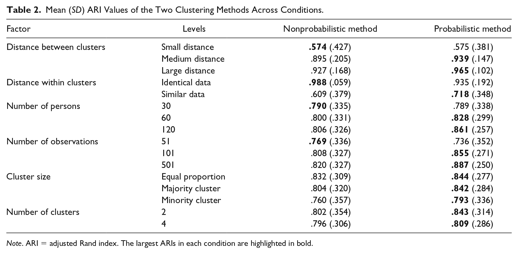
Note. ARI = adjusted Rand index. The largest ARIs in each condition are highlighted in bold.
To gain an insight into effect size, we performed a repeated-measures analysis of variance (RM-ANOVA) on ARI values including all possible two-way interactions. Results are shown in Table 3. Between-method effects give an indication of the general influence of the manipulated factors on membership recovery, while within-data effects illustrate the differential effects of these factors on the two different clustering methods. Effect sizes suggest that low distance between (
Results of a RM-ANOVA Evaluating the ARI Values of Both Clustering Methods.
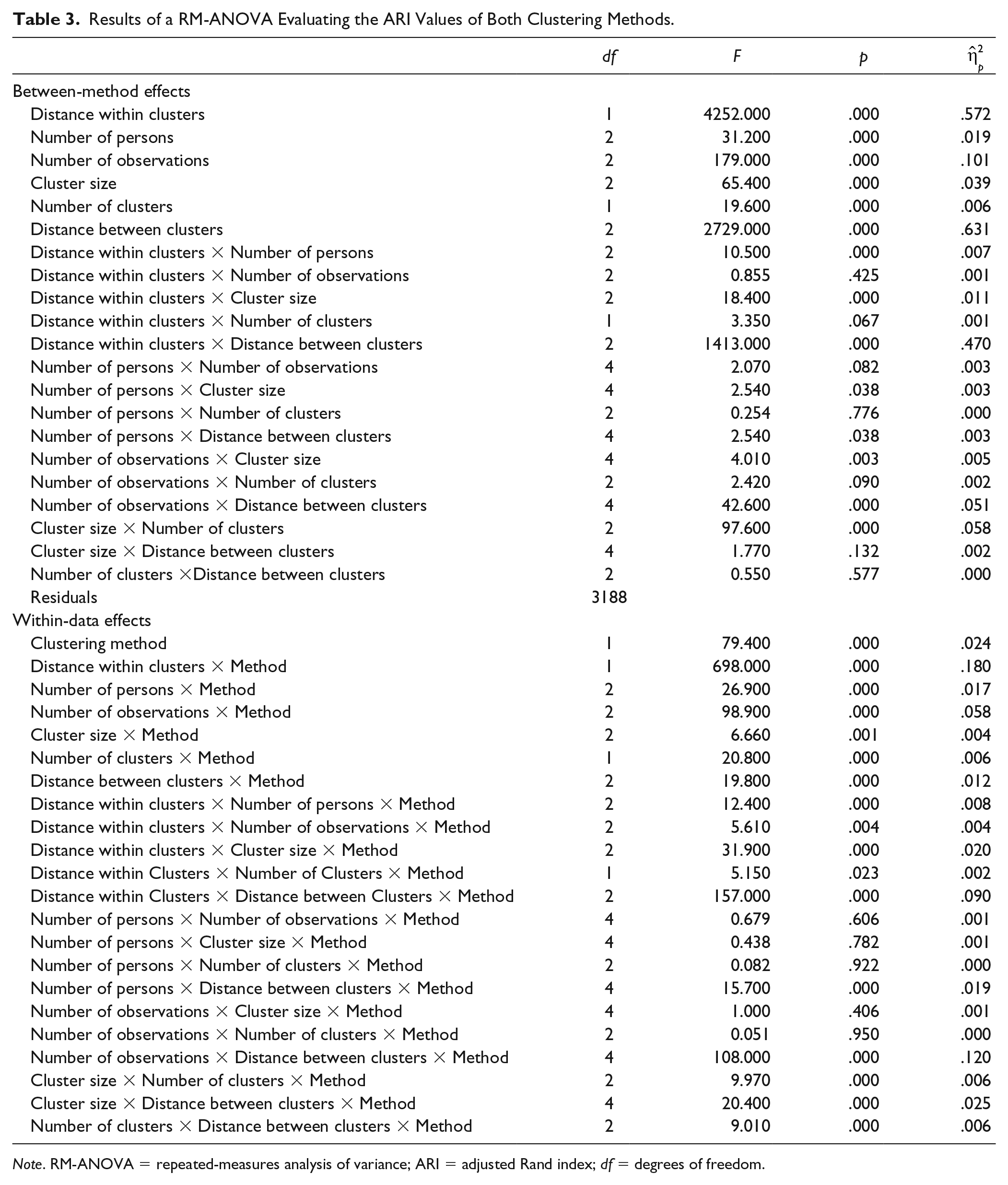
Note. RM-ANOVA = repeated-measures analysis of variance; ARI = adjusted Rand index; df = degrees of freedom.
Recovery of true cluster-specific VAR(1) slopes
Recovery of coefficients was assessed through the mean
10
Euclidean distance between the estimated
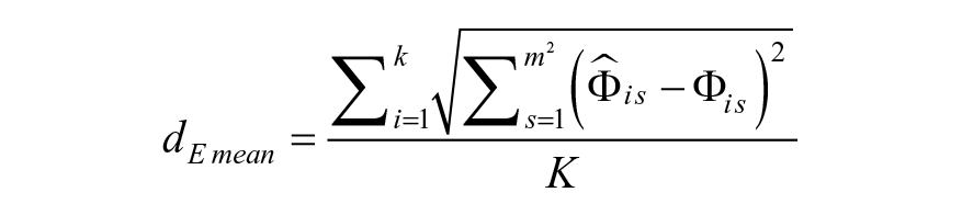
Table 4 shows average mean Euclidean distances across conditions. Again, the probabilistic method shows overall superior recovery over the nonprobabilistic method with mean values of .20 (SD = .15) and .24 (SD = .19), respectively. Table 5 displays the result of a RM-ANOVA on mean Euclidean distances. Effect sizes suggest that the largest influence on parameter recovery is shown for large distance within clusters (
Mean (SD) Euclidean Distances Between True and Estimated VAR(1) Slopes for the Two Clustering Methods Across Conditions.
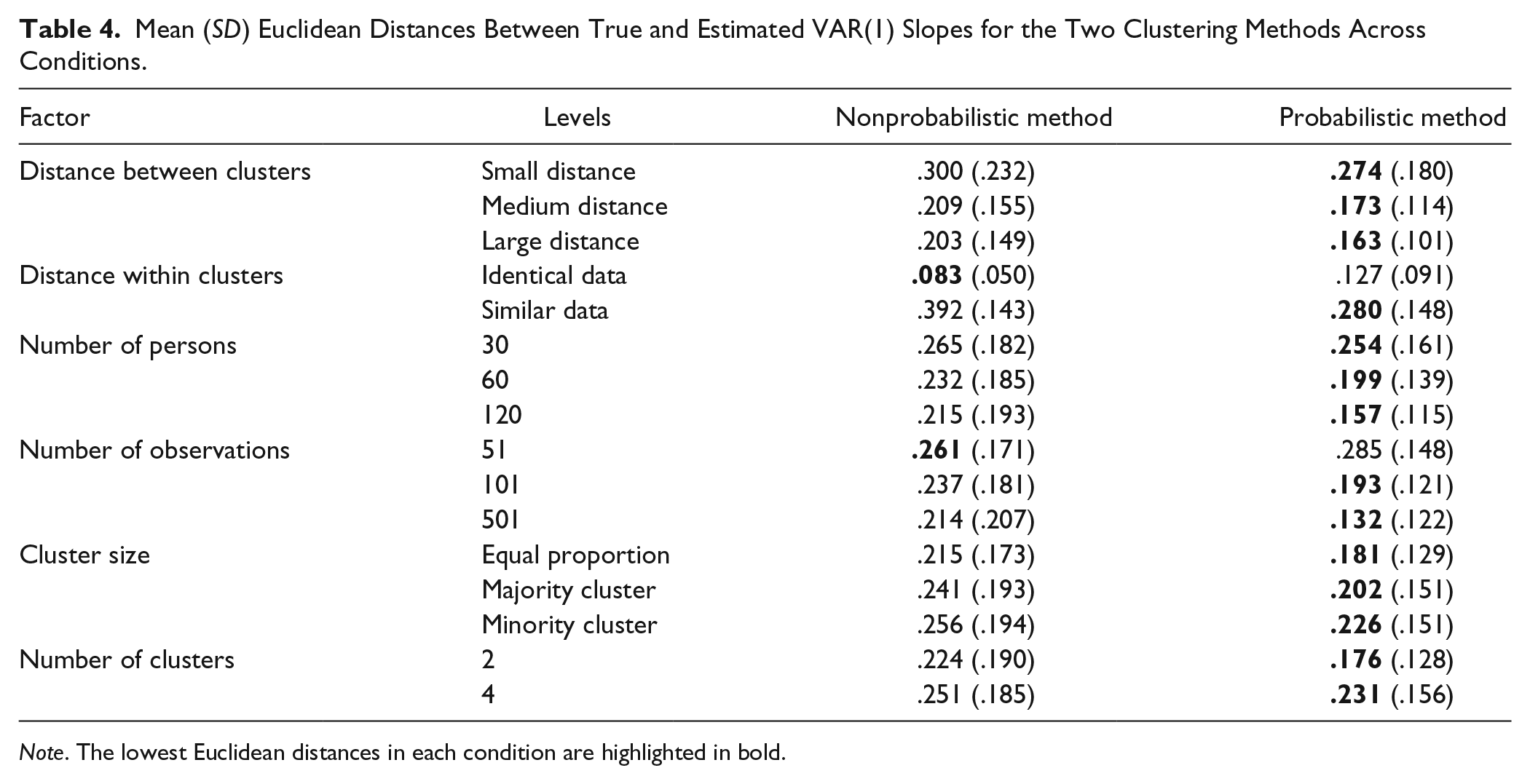
Note. The lowest Euclidean distances in each condition are highlighted in bold.
Results of a RM-ANOVA Evaluating the Mean Euclidean Distances of Both Clustering Methods.
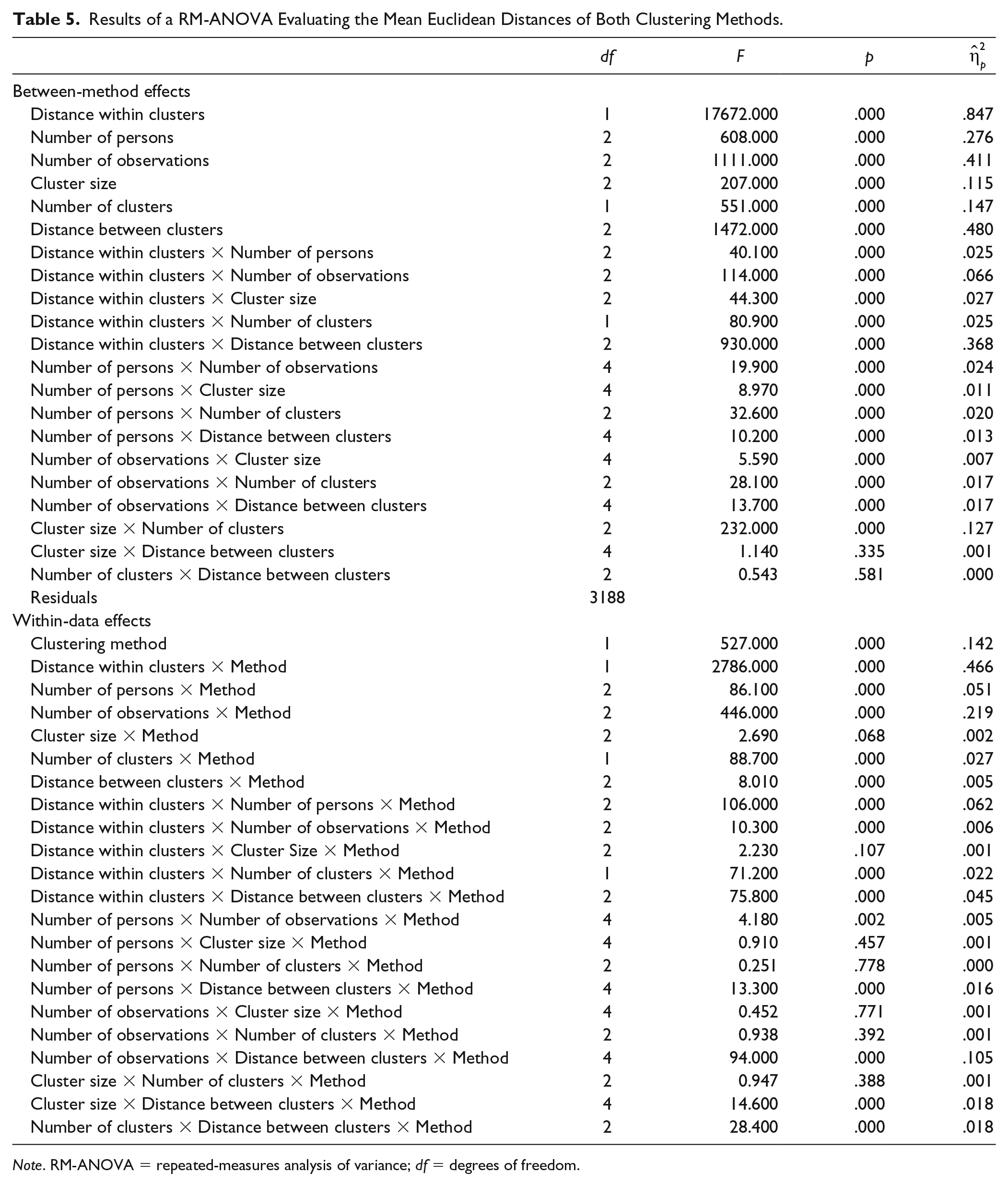
Note. RM-ANOVA = repeated-measures analysis of variance; df = degrees of freedom.
Sensitivity to Local Minima
We also compared clustering methods on attraction rates, the percentage of runs out of the 101 that resulted in the model that was retained as solution. The average attraction rates across simulation conditions are displayed in Table 6 and the RM-ANOVA results in Table 7. Both tables suggest that regardless of the data analyzed, the probabilistic clustering method had much lower attraction rates with a high percentage of runs resulting in a suboptimal solution (
Average Attraction Rates (SD) of the Two Clustering Methods Across Simulation Conditions.
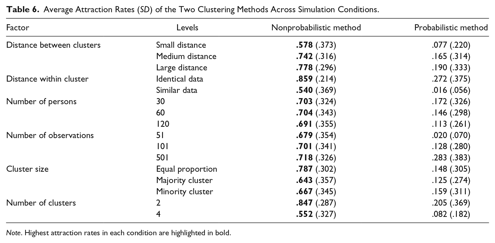
Note. Highest attraction rates in each condition are highlighted in bold.
Results of a RM-ANOVA Evaluating the Attraction Rates of Both Clustering Methods.
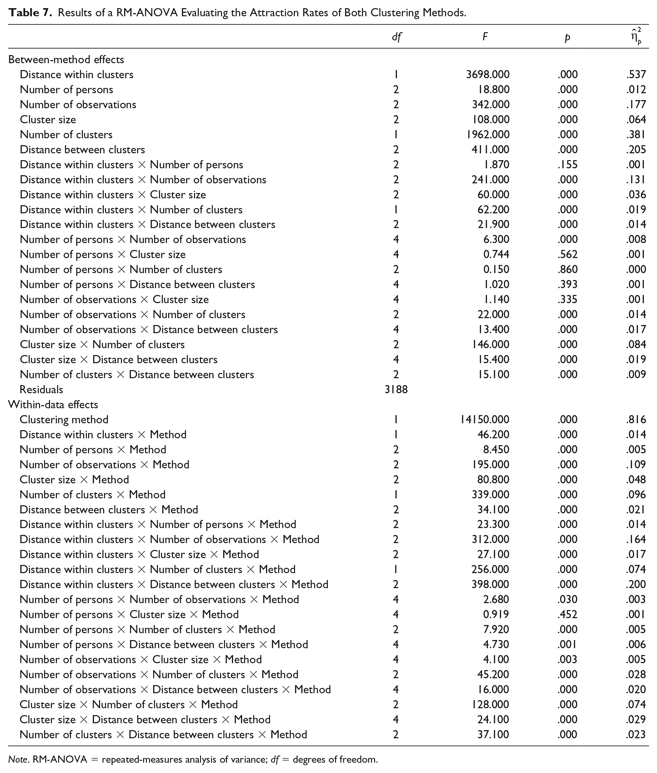
Note. RM-ANOVA = repeated-measures analysis of variance; df = degrees of freedom.
Results Simulation 2
The results of the second simulation are compared with the results of the first simulation’s small differences condition in Table 8. By introducing small differences in intercepts, the performance improved with regard to all three aspects evaluated here, with exception of the attraction rates of the probabilistic clustering method. The improvement is a little smaller than the improvement of increasing the distance in VAR(1) coefficients from small differences to medium differences (cf. the medium distance rows in Tables 2, 4, and 6). Larger distances between the cluster-level intercepts have the potential to improve the performance of the clustering algorithms to an even larger extent.
Differences Between the Simulations With Equal and Unequal Intercepts Between Clusters.
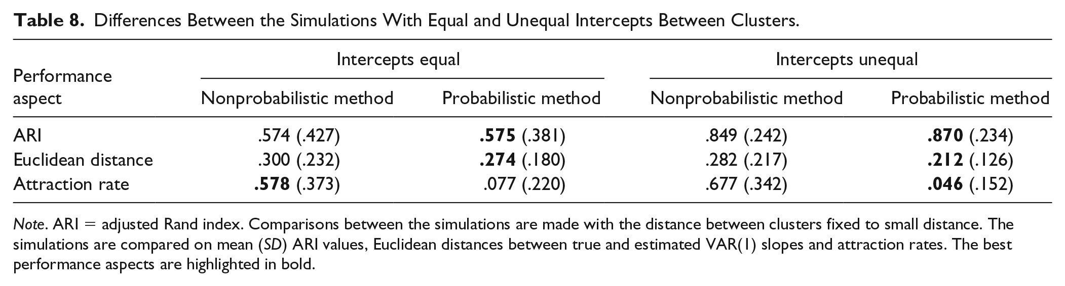
Note. ARI = adjusted Rand index. Comparisons between the simulations are made with the distance between clusters fixed to small distance. The simulations are compared on mean (SD) ARI values, Euclidean distances between true and estimated VAR(1) slopes and attraction rates. The best performance aspects are highlighted in bold.
Discussion of Results
Based on the results of the simulation study, we draw the following conclusions. When true parameters of individuals within a cluster are not identical, the probabilistic clustering method demonstrates better recovery of both cluster membership and VAR(1) slopes than the nonprobabilistic approach. Under the conditions of our simulation, both methods performed well, but the retrieval of cluster parameters and classifications depended crucially on clusters being well-separated. Thus, the distance between clusters is an important predictor for the success of clustering methods, particularly with increasing variation within clusters. It is apparent that clustering methods should be employed only if visible differences between groups can be expected.
Compared with the simpler nonprobabilistic method, the probabilistic clustering method estimates additional parameters, such as the variation within clusters and the cluster proportions. Consequently, a high number of observations and a high sample size are required when this method is employed. While more complex, the estimation of additional parameters by the probabilistic clustering method can offer advantages by providing more information about the data structure. Employing a finite mixture model, the within-cluster variation in dynamics can be estimated. Furthermore, taking estimated proportions into account during the determination of probabilistic cluster membership allowed for improved inferences with regard to cluster classification when proportions were unequal.
An Empirical Example
Data and Modelling Procedure
We applied both clustering methods to the data of the HowNutsAreTheDutch diary study (for details, see Van der Krieke et al., 2016). The data comprises 973 participants who were assessed three times daily (morning/midday/night) over 30 or 31 days. We focus here on participants who completed at least 68 measurements (N = 366). We selected Positive Affect Activation, Positive Affect Deactivation, Negative Affect Activation, and Negative Affect Deactivation (PAA, PAD, NAA, and NAD) as endogenous variables for our analysis. On every measurement, each variable was assessed as the sum score of three items, each item was scored on a continuous scale from 0 to 100. Missing data and values for night measurements were imputed to fulfil the VAR assumption of equidistant time-points. Data were imputed using Amelia II (Honaker, King, & Blackwell, 2011) taking lags of previous and leads of following measurements into account. During the imputation process participants were treated as different cross-sections to account for interindividual differences. To account for possible effects of time of day, each individual time series was centered across the observed mean score of time of day of that individual.
During the first estimation step of the probabilistic clustering method, it was determined that of all 366 participants the time series of 345 were best summarized by a VAR(1), 19 were best described by a VAR(2) and 2 by a VAR(3) model. We decided to apply the probabilistic clustering method for both VAR(1) and VAR(2) models, to keep the dimensionality of parameter vectors,
For the nonprobabilistic method the ideal number of clusters balancing goodness of fit and model complexity was determined with the CHull procedure (Bulteel, Wilderjans, Tuerlinckx, & Ceulemans, 2013; Wilderjans, Ceulemans, & Meers, 2013). The CHull procedure favored the three cluster solution, but the final VAR(1) patterns of different clusters looked similar for other number of cluster solutions.
Cluster solutions were contrasted using relevant cross-sectional individual characteristics that had not been included in the clustering process to find whether the methods were able to differentiate clusters that would correspond to different personality characteristics. Clusters are described in terms of gender proportion, age, positive and negative affect schedule (Peeters, Ponds, & Vermeeren, 1996), anxiety and panic, depression (Quick Inventory of Depressive Symptomatology sum; Rush et al., 2003), self-reported proportion of time spent with others, neuroticism, extraversion, and openness (de Fruyt & Hoekstra, 2008); for details, see Van der Krieke et al. (2016).
Empirical Results
Mean VAR coefficients of the clusters probabilistic VAR(1) and VAR(2) clusters are shown in Figure 2. A comparison of Figures 2 (a) and 2 (b) shows that lag 2 coefficients fade once they are averaged across people with similar dynamics. Furthermore, clustering methods based on VAR(1) coefficients appear better able than the VAR(2) clustering solution at distinguishing groups of individuals with different personality characteristics relating to positive and negative affect. Table 9 and Figure 3 give the cluster-wise mean scores on cross-sectional measures for the probabilistic VAR(1) solution. To illustrate the potential of the probabilistic clustering method, we focus on the probabilistic VAR(1) 5 cluster solution in Table 9 (and Figure 2 (a)). Detailed results for the nonprobabilistic clustering model and the probabilistic VAR(2) model are shown in the supplementary material available online, so is the estimated within-cluster variance for the probabilistic VAR(1) method.
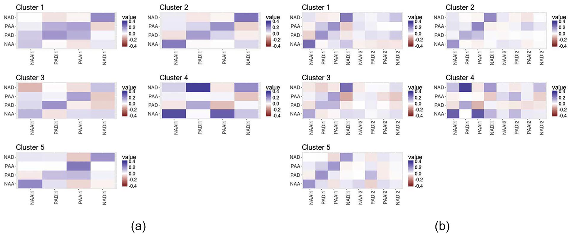
Clusters are based on the multivariate associations between the following variables: Negative Affect Deactivation (NAD), Positive Affect Activation (PAA), Positive Affect Deactivation (PAD), and Negative Affect Activation (NAA). (a) Mean VAR(1) coefficients per cluster, reached through the probabilistic VAR(1) clustering method. (b) Mean VAR(2) coefficients per cluster, reached through the probabilistic VAR(2) clustering method.
Mean (SD) Scores on Static Variables for the Clusters Reached by the Probabilistic Clustering VAR(1) Method.
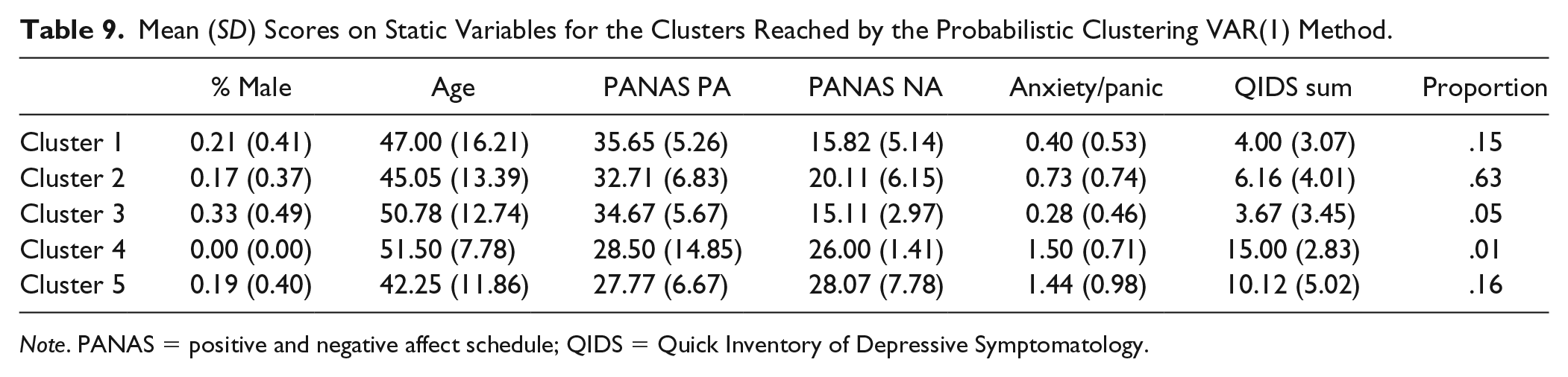
Note. PANAS = positive and negative affect schedule; QIDS = Quick Inventory of Depressive Symptomatology.
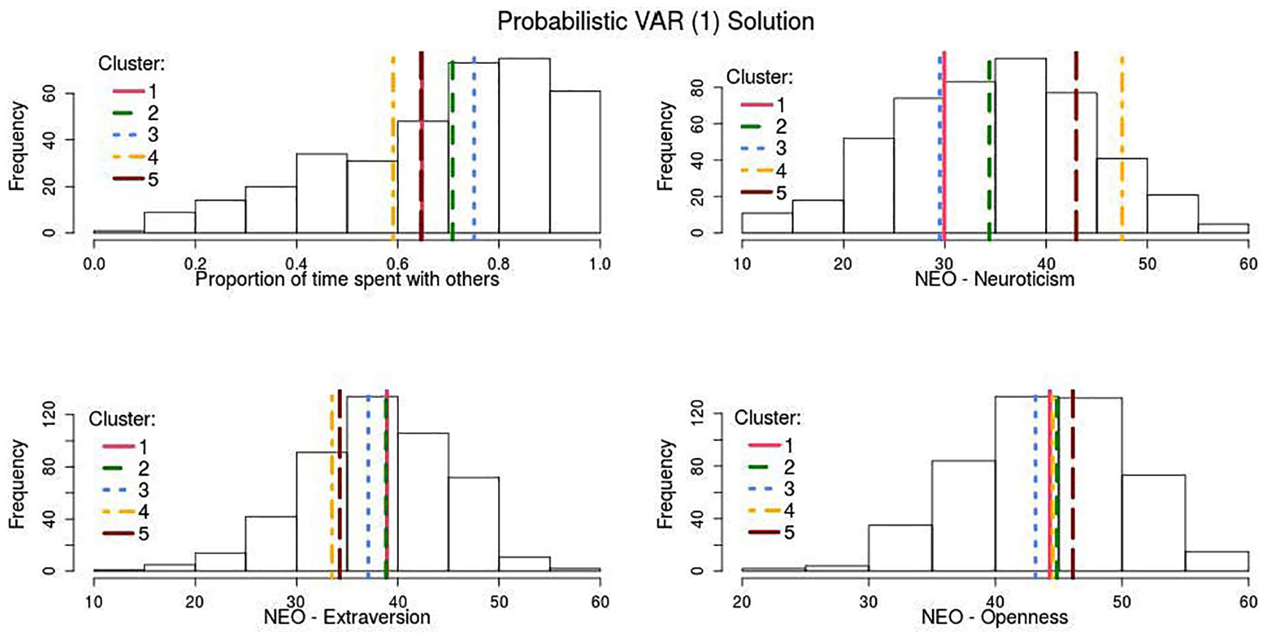
Distribution of scores on personality measurements of the whole sample.
The estimation of within-cluster variance with regard to the parameters distinguishes the proposed method from the other time series clustering methods discussed in the introduction. These estimates allow to evaluate which variables differ most markedly between clusters relative to their within-cluster variance. This provides insight into the between-cluster differences that drive our cluster solution. With regard to VAR coefficients the lagged effect of NAA on PAA had the highest within-cluster variance with a SD of 0.173; the lagged effect of NAD on NAA had the smallest within-cluster variance with a SD of 0.118 (see Table 15 in the supplementary material available online). For the intercepts, the within-cluster SD varied from 53.123 (PAA) to 39.506 (NAA). Thus, a deviation of one SD from a cluster mean coefficient would require a difference between 0.173 and 0.118 in VAR coefficients or a difference between 53.123 and 39.506 in intercepts.
The probabilistic cluster memberships give direct indication of the classification uncertainty of every person. The classification uncertainty, the probability that an individual has been misclassified (i.e., 1 − max(
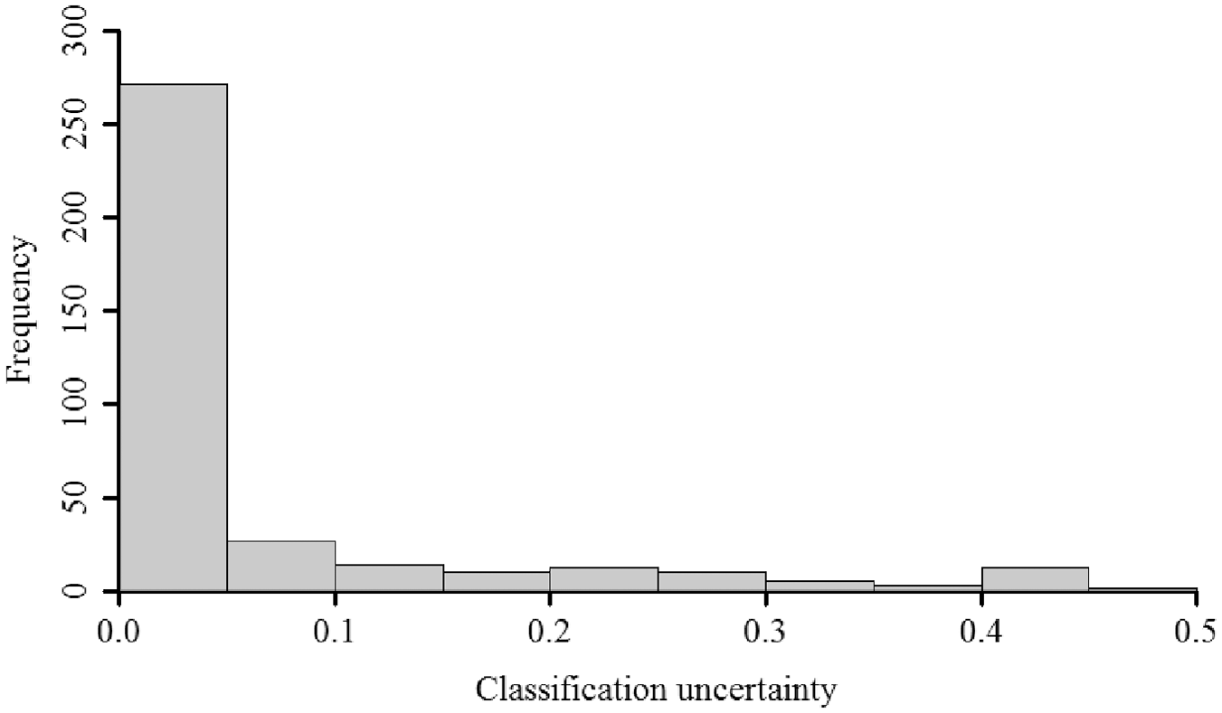
Classification uncertainty for all 366 participants in the solution reached by the probabilistic VAR(1) clustering method.
Emotions are intensive and transient subjective states that emerge in response to specific stimuli and are typically described in terms of an affective valance dimension (positive to negative affect or PA/NA) and an arousal dimension (low-to-high bodily activation; Russell, 1980). Both dimensions are combined in our operationalization of activated or high arousal PA (energetic/enthusiastic/cheerful), deactivated or low arousal PA (relaxed/content/calm), activated NA (anxiety/nervous/gloomy), and deactivated NA (gloomy/dull/tired). Below we will interpret the five clusters.
The Majority Cluster 2
The majority of our participants were in Cluster 2 (63%), which can therefore be used as a point of reference for the interpretation of the other clusters. Cluster 2 shows comparatively average PA and NA levels (see Table 9) with relatively high autocorrelations (see Figure 2) for activated and deactivated PA (.19/.17) and NA (.24/.25); thus relatively persistent and stable emotions over time and situations. External criteria (in Figure 3) are consistent with these observations and show comparatively high extraversion scores (closely aligned to PA), also reflected in the proportion of time spend with other people, and average neuroticism levels (closely aligned with NA; John, Robins, & Pervin, 2008). Temporal cross-valence correlations between PA and NA were rather weak (.04 to −.07, see Table 10), which might suggest two relatively independent within-person affect dimensions rather than a bipolar (PA ↔ NA) dimension, in line with previous work (Rush & Hofer, 2014; Russell & Carroll, 1999). However, it is salient that most cross-regressive associations were close to zero. This might be indicative of individual differences in cross-regressive effects that are cancelled out once effects are aggregated across individuals with similar dynamics. Alternatively, this could be seen as support for the notion that cross-regressive effects found through ideographic methods are often the result of overfitting (Bulteel, Mestdagh, Tuerlinckx, & Ceulemans, 2018).
Mean VAR Coefficients of the Probabilistic Clustering VAR(1) Method.
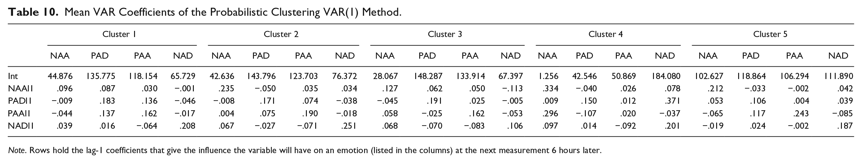
Note. Rows hold the lag-1 coefficients that give the influence the variable will have on an emotion (listed in the columns) at the next measurement 6 hours later.
Positive Affect Cluster 1
When we shift focus to the Cluster 1 participants (15%) they combine high average PA and relatively low NA, which is indicative of high emotional well-being (Diener, Scollon, & Lucas, 2009). These high PA scores align with comparatively high extraversion scores (see Figure 3), whereas low NA concedes with low neuroticism (also called emotional stability). In terms of emotion dynamics (see Table 10), Cluster 1 people experienced shorter lived activated NA than people in Cluster 2 (such as anxiety, .10 vs. .24), while their deactivated NA (such as weariness) and PA stabilities were comparable. Also, the temporal link between PA and NA was comparable to Cluster 2 (.10 to −.06, see Table 10).
Well-Adjusted Cluster 3
Cluster 3 captures the 5% of the participants who were emotionally most stable and well-adjusted, as reflected in their comparatively low symptom levels of anxiety and depression (Table 9). The relatively high PA and low NA scores indicate high emotional well-being, and are in keeping with low neuroticism (i.e., emotional stability) and intermediate extraversion (see Figure 3). In terms of emotion dynamics Cluster 3 participants showed comparatively short-lived NA stability (activated .13, deactivated .11), compared with Cluster 2, but comparable PA stabilities (.16 and .19) and temporal cross-valence correlations (.06 to −.08).
Depressed Cluster 4
Cluster 4 was rather small (1%) and captured two participants with comparatively high symptom levels of depression and anxiety, high NA and low PA (i.e., low emotional well-being). Unsurprisingly, Cluster 4 participants reported highest neuroticism and lowest extraversion levels (Figure 3), and spend most time alone. In terms of emotion dynamics their activated NA (.33) showed higher autocorrelation compared with the other clusters, whereas the stability of their activated PA was remarkably low (.02), which is in line with having a depressed mood (Watson, Clark, & Tellegen, 1988). Another unusual pattern was the strong temporal link between activated NA and PA (.30) and deactivated NA and PA (.37); When these participants felt relaxed/content (deactivated PA), they were more likely to be tired or gloomy (deactivated NA) 6 hours later. Overall, the results suggest that Cluster 4 people showed affective experiences with a stronger temporal relationship and a more bipolar nature.
High Arousal Positive Affect Cluster 5
Cluster 5 captured 16% of the participants who reported relatively high depressive and anxious symptom levels and high NA, but also high PA, in contrast to Cluster 4 (Table 9). Cluster 5 participants were relatively high on neuroticism, although somewhat less than Cluster 4 people, and reported relatively low extraversion, but high openness (Figure 3). In terms of emotion dynamics the autocorrelations for activated and deactivated NA (.21/.19) were somewhat weaker but comparable to Cluster 2. However, the stabilities for activated PA was somewhat stronger (.24 vs. .19) but the stability of deactivated PA somewhat weaker (.11 vs. .17) than for Cluster 2. Cluster 5 participants reported relatively persistent high arousal positive experiences, in line with their younger age, but not with their comparatively low extraversion. The temporal cross-valence correlations (.06 to −.09) were not unusual, and supported relatively independent (or bivariate) affect dimensions.
Overall, relatively distinct affect dimensions were observed, except in Cluster 4. This is in line with previous research (Rush & Hofer, 2014) reporting on inversely correlated PA and NA factors at the within-person level and two independent PA and NA factors at the between-person level. As can be seen in Table 9 and Figure 3, provided that the SD of correlations is typically about four times larger within individuals than for groups (Fisher, Medaglia, & Jeronimus, 2018), these results stress the importance of accounting for both measurement levels and using within-person dynamics when clustering on between-person differences.
Conclusion
Dynamic clustering procedures might fill the methodological gap in time series analysis by allowing drawing accurate generalizations from intensive longitudinal data while accounting for qualitatively different processes between individuals. Employing probability distributions to model within-cluster variation appears a promising avenue for psychological research where most investigated constructs are assumed to be represented on a continuum with individuals displaying similar, but hardly ever equal dynamics. The probabilistic clustering method addresses two issues of concern inherent to the dynamic clustering of human data: (a) human data is likely to be characterized by variation within clusters and (b) most individual properties investigated in the social sciences cannot be assumed to occur in balanced proportion across the population.
Supplemental Material
Supplementary_Material_asmnt – Supplemental material for Insight Into Individual Differences in Emotion Dynamics With Clustering
Supplemental material, Supplementary_Material_asmnt for Insight Into Individual Differences in Emotion Dynamics With Clustering by Anja F. Ernst, Marieke E. Timmerman, Bertus F. Jeronimus and Casper J. Albers in Assessment
Footnotes
Declaration of Conflicting Interests
The author(s) declared no potential conflicts of interest with respect to the research, authorship, and/or publication of this article.
Funding
The author(s) disclosed receipt of the following financial support for the research, authorship, and/or publication of this article: This work was supported by the Netherlands Organisation for Scientific Research (NWO), grant numbrt 406.17.510.
Supplemental Material
Supplemental material for this article is available online.
Notes
References
Supplementary Material
Please find the following supplemental material available below.
For Open Access articles published under a Creative Commons License, all supplemental material carries the same license as the article it is associated with.
For non-Open Access articles published, all supplemental material carries a non-exclusive license, and permission requests for re-use of supplemental material or any part of supplemental material shall be sent directly to the copyright owner as specified in the copyright notice associated with the article.