Sage Journals: Discover world-class research

Abstract

Political advertising on digital platforms has grown dramatically in recent years as campaigns embrace new ways of targeting supporters and potential voters. We examine how political campaign dynamics have evolved in response to the growth of digital media by analyzing the advertising strategies of US presidential election campaigns during the 2020 primary cycle. To identify geographic and temporal trends, we employ regression analyses of campaign spending across nearly 600,000 advertisements published on Facebook. We show that campaigns employed a new strategy of targeting voters in candidates’ home states during the “invisible primary.” In contrast to earlier studies, we find that home state targeting is a key strategy for all campaigns, rather than just for politicians with existing political and financial networks. While all candidates advertised to their home state, those who dropped out during the invisible primary tended to spend disproportionately more than the candidates who outlasted them. We also find that as the first wave of state caucuses and primary elections approach, campaigns shift digital ad expenditures to states with early primaries such as Iowa and New Hampshire and, to a lesser extent, swing states.

Keywords

political advertising digital media campaign strategies Facebook

Introduction

In recent years, presidential campaigns in the United States have shifted from traditional forms of advertising—such as television, radio, and print—to digital media. Historically, campaigns have spent the largest proportion of their advertising budgets on television commercials, as they are most effective in reaching a large number of voters. However, the proportion of ad spending devoted to television has declined in each election year since 2008 (Cassino, 2017). Over the same period, the proportion spent on digital advertising increased from 0.2% to 14.4% in 2016 and was projected to account for 28% of political ad spending in 2020 (see Figure 1). In fact, the campaign of Joe Biden, the winner of the Democratic nomination and general election, spent 30.7% of its ad budget on Facebook and Google ads alone (Center for Responsive Politics, 2020). The strategic decisions that campaigns make about advertising—where, when, and how to deploy ads—are critical to understand given their influence on electoral outcomes (West, Kern, Alger, and Goggin, 1995).1

Figure 1.

Online advertising has become more central to political advertising budgets, from below 1% in 2008 to 14.4% in 2016. It was projected to reach 28% in 2020 and surpass the combined spending on political ads in press, radio, direct mail, telemarketing, and others (Cassino, 2017).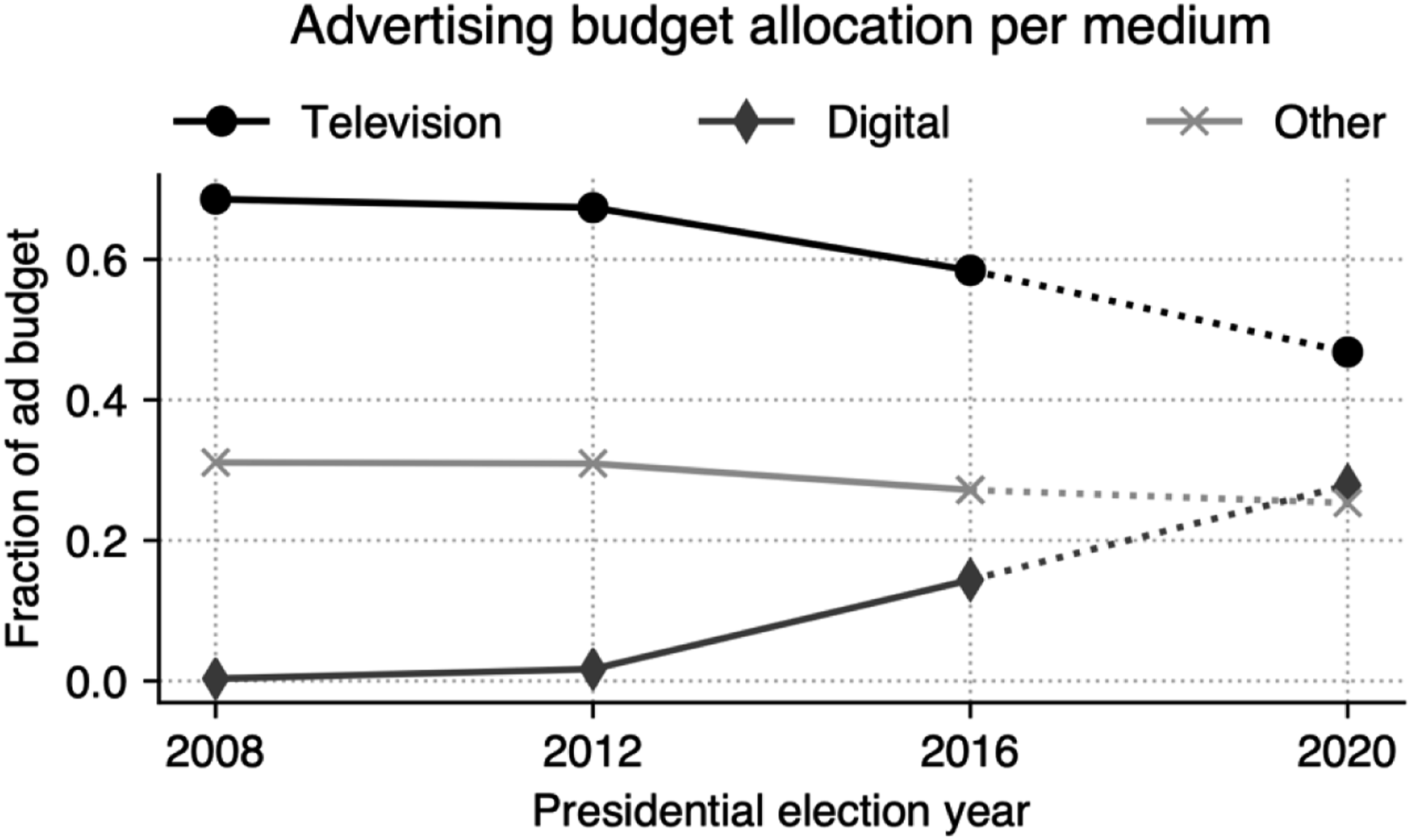

Digital advertising has a number of advantages over television and other traditional media. Most importantly, it allows campaigns to precisely target voters using a range of tools made available to them by ad platforms. Campaigns can choose the target audience based on their location, age, and gender, as well as a number of interest-based parameters such as inferred political alignment. They can also target particular users based on their personally identifiable information (PII), such as email addresses, phone numbers or names, as well as promote ads to other users similar to those whose PII they’ve obtained (Martinez, 2018). By clicking, commenting, or sharing ads, social media users provide campaigns with immediate feedback on ads’ ability to engage potential voters; the campaigns, in turn, can use it to more efficiently allocate resources (Erdody, 2018; Kreiss, Lawrence, and McGregor, 2018). Campaigns can advertise on digital platforms with relatively small budgets, in contrast to television advertising where budgets can run from hundreds of thousands to millions of dollars. Due to their lower cost, digital ads have served as an equalizing force for long-shot candidates (Christenson, Smidt, and Panagopoulos, 2014; Paolino and Shaw, 2003).

Despite dramatic growth in digital advertising, scholars know little about how political campaigns leverage its unique features. To address this gap, we consider two questions. First, we investigate whether campaigns target voters by location in a manner consistent with traditional forms of advertising. Second, we investigate whether campaigns’ advertising strategies shift over time as they consider the next immediate need. To answer these questions, we examine Facebook advertising by US presidential campaigns during the 2020 primary election cycle. Facebook accounts for the largest share of digital advertising due its ease of use and the size of its user base (Erdody, 2018), and experiments demonstrate that ads hosted on the platform can lead to increased political participation (Haenschen and Jennings, 2019). Using the Facebook Political Advertising Library (Facebook, 2019), we analyze nearly 600,000 advertisements published by 26 Democratic presidential primary campaigns from 1 January 2019 through “Super Tuesday,” 3 March 2020. After that date only five candidates remained in the race for the nomination. For each ad, the library reports the estimated number of impressions—the number of times that the ad appeared in users’ feeds. In addition to estimated impressions, the library reports the approximate cost, as well as the locations and demographic characteristics, such as age and gender, of users who viewed each ad.

Research on campaign advertising strategies has utilized a range of data sources, the most prominent being television advertising archives (Fowler, Franz, and Ridout, 2017; Goldstein, Niebler, Neilheisel, and Holleque, 2011). These archives collect and encode data on television ads across 210 designated market areas (DMAs), including location, cost, and content. Since some DMAs span multiple states, this data has limited utility for analyzing advertising strategies by state. Because states award both primary delegates and general electors, state-level outcomes are important for answering questions about presidential campaign strategies. The Facebook Ad Library provides the same level of detail, but also allows us to compare state-level advertising by each campaign over time.

We find that campaigns introduced a new dynamic strategy: home state advertising. Early in the primary season, campaigns spend a larger share of their budget in the candidate’s home state where digital advertising helps to raise money, signal viability, and build momentum. In contrast to earlier studies showing that candidates’ home states allow them to tap into existing political and financial networks, we find that all candidates advertised heavily in their home states, regardless of the size of their existing constituency or network. Candidates who dropped out during the invisible primary invested much more heavily in home state advertising than the candidates who outlasted them—despite an attempt, we argue, to elevate their profiles by qualifying for the Democratic debates. We also find that as the first wave of state caucuses and primary elections approach, campaigns shift digital ad expenditures to states with early primaries such as Iowa and New Hampshire and, to a lesser extent, swing states.

The remainder of the paper is organized as follows. In Section 2, we provide an overview of strategies that campaigns employ to win primaries. Section 3 covers key elements of digital advertising on Facebook. Sections 4 and 5 provide an overview of the data and methodology, respectively. In Section 6 we discuss the results of our analyses of primary advertising strategies. Section 7 concludes with broader implications for primary dynamics.

Political Advertising Strategies

How do presidential candidates win primaries? This question has been the subject of considerable debate since the modern era of presidential nominations began in 1972. The dominant view that campaigns must persuade and mobilize the voting public has given way to the perspective that the elites, interest groups, and donors comprising political parties are the most consequential audience for campaigns (Cohen, Karol, Noel, and Zaller, 2008). However, from the campaign’s perspective, the same dynamics are present: money, media coverage, poll rankings, and endorsements shape nomination outcomes (Aldrich, 2009; Dowdle, Adkins, and Steger, 2009). Candidates allocate their resources strategically—deciding where and how to compete—given party rules, timing, and their competitive status relative to other candidates (Aldrich, 1980; Bartels, 1988; Gurian, 1986). The most critical of these strategic maneuvers takes place in the year prior to the first primary contest—a period known as the “invisible primary” (Aldrich, 2009; Cohen et al., 2008).

The structure of the nomination process—a series of state contests followed by a convention—favors a dynamic strategy that evolves as resource levels and candidate fortunes change. Campaigns develop a state-level allocation strategy in order to maximize delegates (Bartels, 1985), recognizing the positive relationship between campaign expenditures and vote share (Grush, 1980). States with large numbers of delegates are attractive to all candidates (Bartels, 1985), as are states with early enough contests to signal momentum or front-runner status (Adkins and Dowdle, 2001; Bartels, 1988). However, individual states present different opportunities to different candidates. Campaigns allocate expenditures on the basis of whether a state holds caucuses or a primary, whether delegates are distributed proportionally or winner-take-all, as well as a host of demographic and geographic factors (Gimpel, Lee, and Kaminski, 2006; Lin, Kennedy, and Lazer, 2017; Ridout, Rottinghaus, and Hosey, 2009). We utilize campaigns’ growing use of digital advertising to investigate these strategies during the invisible primary.

The length of the nomination calendar influences candidates’ resource levels. Candidates focus on raising money throughout the primary cycle, as the amounts raised and in cash reserves are reliable predictors of winning the primary election (Adkins and Dowdle, 2001; Brown Jr, Powell, and Wilcox, 1995). Campaigns with a greater web presence receive more contributions (Christenson et al., 2014), so we expect campaigns to also use digital advertising for fundraising. We posit that campaigns will concentrate their digital advertising efforts in candidates’ home states, where they are most well known and contributions are most likely. Studies suggest that candidates with large electoral constituencies, such as current or former governors or senators, have the most pronounced home state fundraising advantage (Adkins and Dowdle, 2002; Brown Jr et al., 1995; Hinckley and Green, 1996). Hypothesis 1: Campaigns target contributors in their home states.

During the general election, campaigns allocate their resources based on whether a state is considered a battleground or part of the party base (Shaw, 1999, 2006). Primary dynamics may or may not follow the logic of the general election with respect to delegates in battleground or “swing” states. For example, a recent study shows that campaigning in uncontested states can lead to increased campaign contributions (Urban and Niebler, 2014). However, candidates may pursue a secondary goal of engaging and educating voters in the states that will be most consequential for the general election (Gimpel, Kaufmann, and Pearson-Merkowitz, 2007). What voters learn about candidate ideologies during the primary influences their subsequent support (Hirano, Lenz, Pinkovskiy, and Snyder, 2015; Knight and Schiff, 2010). We consider whether campaigns begin advertising in swing states in order to establish momentum going into the general election. Hypothesis 2: Campaigns target voters in swing states.

The ordering of primaries influences the perceived electoral value of particular states. Voters’ and parties’ perceptions of candidates evolve over the course of the primary season, resulting in momentum for some candidates and decay for others (Bartels, 1988; Knight and Schiff, 2010). For lesser known candidates, winning the earliest primaries is a key strategy (Paolino and Shaw, 2003). The nomination of Barack Obama in 2008 has been attributed in part to his campaign’s use of digital advertising to establish early momentum (Aldrich, 2009). A study of primaries conducted between 1980 and 1996 shows that the New Hampshire primary, which takes place early in the primary season, is correlated with the ordinal ranking of candidates (Adkins and Dowdle, 2001). Therefore, we expect campaigns to target states holding the first few primaries in February. We also expect campaigns to target the large number of states that hold primaries on Super Tuesday, a date which occurs early in the primary season and allocates the largest number of delegates (Almukhtar, Martin, and Stevens, 2019). Hypothesis 3: Campaigns target voters in states with early primaries.

Fundraising begins early on to allow candidates to build their organizations, remain competitive, and survive setbacks (Adkins and Dowdle, 2002; Goff, 2004; Hinckley and Green, 1996; Smidt and Christenson, 2012). Fundraising also sends important signals about candidate viability. Candidates periodically report their fundraising totals to the Federal Election Commission (FEC), allowing both parties and the public to gauge whether candidates have adequate financial support. During the 2020 season, the Democratic National Committee required candidates to meet specific fundraising and polling thresholds in order to participate in televised debates (Scherer, 2019). We expect that home state ad expenditures will be most pronounced prior to the first debate, when outsider candidates seek to educate the public about their candidacy, and when all candidates seek to maximize fundraising. After the debates, we expect campaigns to target states based on their electoral value. Hypothesis 4: Campaigns’ geographic targeting shifts over time from home states to states with early primaries.

Advertising on Facebook

One of the major differences between online ad platforms and the traditional media is the precision with which the advertiser can describe their ideal audience. Beyond basic demographics such as age, gender, and location, one can also target by inferred interests, including political leaning. Combining several targeting options at once to refine the audience is often referred to as microtargeting. For example, a political campaign might upload the list of people who signed up for their newsletter, ask Facebook to find users who “look alike” (but have not yet signed up), and further refine that audience to target the middle-age and older populations who are historically more likely to vote. The campaign might also use publicly available voter registration data to create a custom audience consisting of registered voters of the opposing party, and then discourage those people from voting. Campaigns’ real-world use of these features has been discussed in the popular press but remains understudied (Lapowsky, 2018; Martinez, 2018).

This study utilizes data from Facebook, which reports all political advertisements published on its platform going back to May 2018. There are two distinct steps in the life-cycle of an ad on Facebook: creation and delivery. During ad creation, the advertiser sets the budget, designs the appearance of the ad—including its text, media (image or video), and the link that the users will open upon clicking the ad—and specifies where, when, and to whom the ad should be shown. The advertiser can target users by their demographic information and location, inferred interests, personally identifiable information, or any combination of those.

Facebook runs live auctions to determine which ads users see. While these auctions were traditionally based only on how much the advertisers were bidding, Facebook now considers many additional factors, among them, the inferred relevance of the ad to a particular user. As a result, ads deemed relevant to users might win the auctions with lower bids, whereas apparently less relevant ads might be financially penalized. Such auctions encourage advertisers to create more relevant content, potentially creating a better online experience for the users, but can also lead to price discrimination and skewed delivery of ads (Ali, Sapiezynski, Korolova, Mislove, and Rieke, 2021).

Data

We use the Facebook Ad Library, the platform’s official Application Programming Interface (API), to programmatically obtain ads published by 26 official presidential campaign accounts.¹ Data for each ad include its creative elements (text, link, and image or video) as well as rough delivery statistics: start time, estimated spend, estimated impressions, gender and age breakdown, and geographical breakdown. See Figure 2 for an example of the Library’s web interface. In total, our dataset contains 571,705 ads.

Figure 2.

Sample web interface from the Facebook Advertising Library.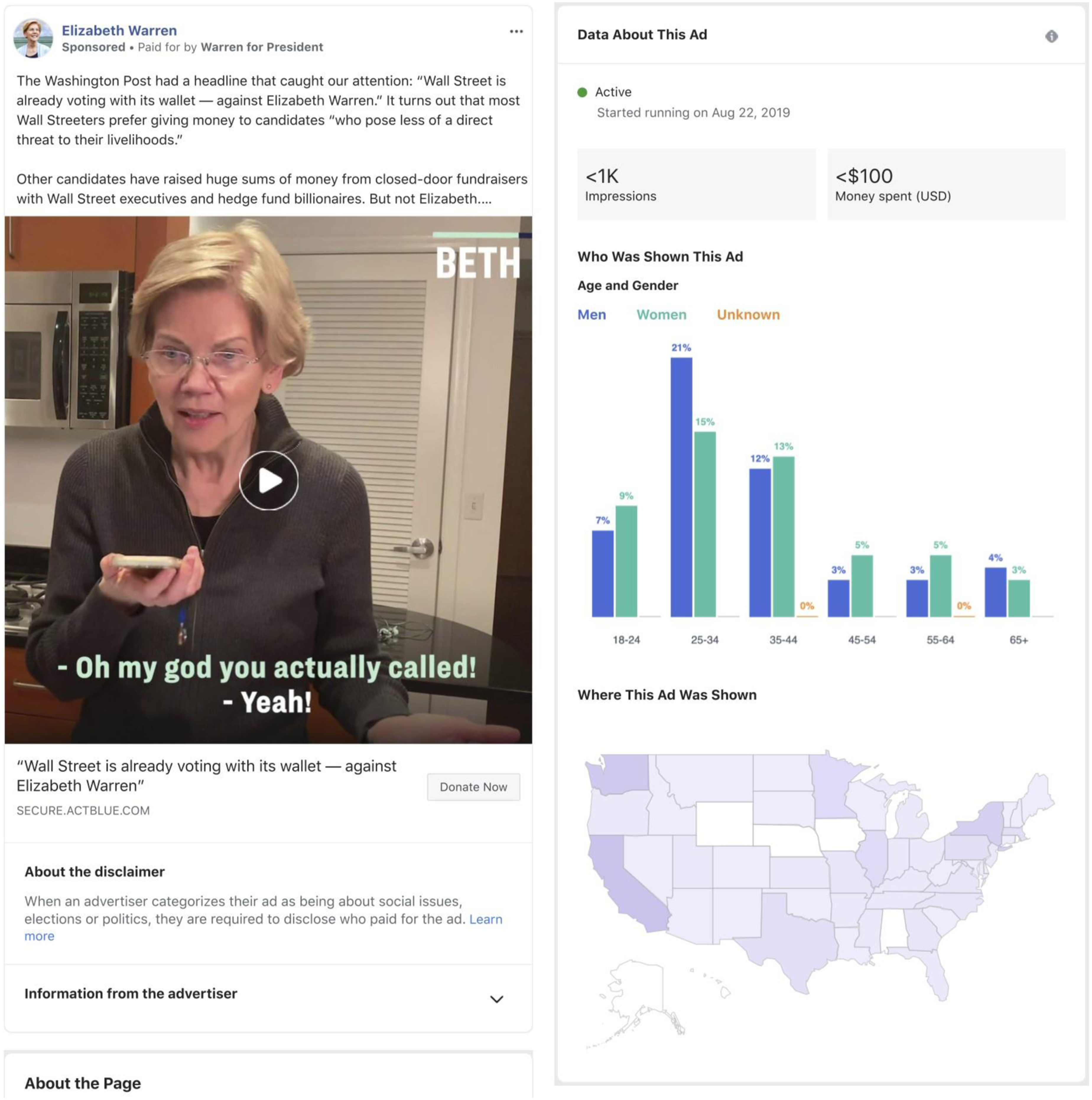

The Facebook Ad Library provides information about the location and demographics of the audience that ultimately saw each ad, but not of the audience that the advertiser targeted. Academic attempts at gathering targeting information from Facebook have been met with legal threats (Lapowski, 2021). The distinction is important to make because unless the advertiser specifies a budget that allows them to reach the entire targeted audience, each ad is only shown to a subset. As we explain above, this subset is not selected strictly randomly. Instead, Facebook attempts to preferentially show the ads to those users who Facebook deems relevant. As a result, it is not possible to directly observe how much of the differences in geographical distribution of the ads is due to a campaign’s deliberate strategy. The delivery statistics are, instead, only a proxy for campaign targeting. Still, based on the information that is available in the Ad Library, we find strong evidence that advertisers target users by location and that this targeting is the leading factor in delivery. If the effect were fully attributable to content-based optimization, we would see that similar ads deliver to similar demographics; however, this is not the case. We observe sets of ads with identical content, yet each delivering to audiences located in different states. We also note that 43% of ads in our dataset were each delivered in only one state (see Figure 3). Despite the fact that more than 80% of ads have budgets lower than $100, this single state effect is not entirely explained by low budgets: 35% of ads with budgets above $500 are still delivered in one state only. Facebook’s delivery algorithm would be unlikely to deem an ad exclusively relevant to people in a particular state without clear direction from the advertiser. Therefore, we conclude that deliberate geographic targeting by campaigns is a driving factor in the effects that we observe.

Figure 3.

87% of all ads cost less than $100 to run. At the same time nearly 43% of all ads in the archive are shown in one state only and only 11% are shown in every state. The high fraction of single state ads is not just an artifact of small budgets: 35% of ads with budgets higher than $500 are only delivered in one state. 10% of single state ads are shown in the candidate’s home state.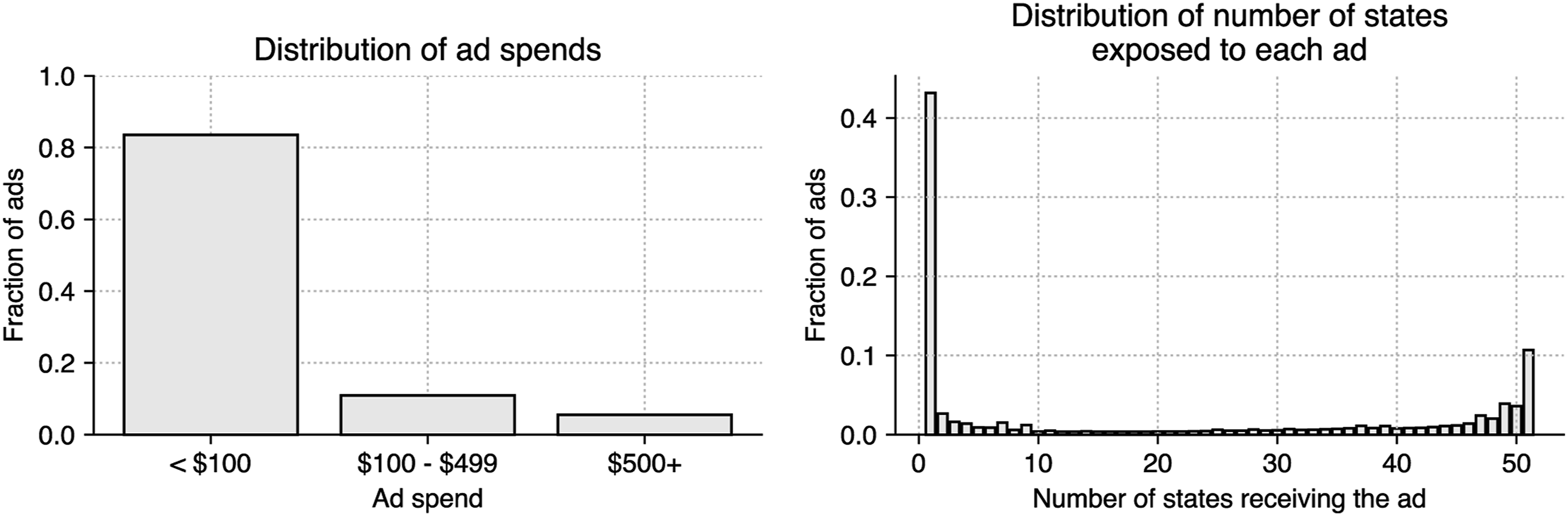

Candidate Characteristics

We define major candidates to be those that reported at least $100,000 in contributions from individuals other than the candidate. A historically large number of major candidates participated in the 2020 Democratic primary: 26, in contrast to five in 2016 and eight in 2008 (US Federal Election Commission, 2020).² As shown in Table 1, our sample includes candidates from 18 states. Most were current or former elected officials at the federal (16), state (3), or local (4) level; just three candidates entered the race with no executive or legislative experience. We also report the date that each candidate suspended their campaign, if applicable. Roughly half campaigned throughout the invisible primary period, with the remaining dropping out in late 2019.

Table 1.

Major democratic presidential candidates.

Candidate	Home State	Highest Elected Office	Suspended Campaign
1 Amy Klobuchar	Minnesota	US Senator	2 March 2020
2 Andrew Yang	New York	—	11 February 2020
3 Bernie Sanders	Vermont	US senator	8 April 2020
4 Beto O’Rourke	Texas	US Representative	1 November 2019
5 Cory Booker	New Jersey	US Senator	13 January 2020
6 Elizabeth Warren	Massachusetts	US Senator	5 March 2020
7 Eric Swalwell	California	US Representative	8 July 2019
8 Jay Inslee	Washington	Governor	21 August 2019
9 John Hickenlooper	Colorado	US Senator	15 August 2019
10 John K. Delaney	Maryland	US Representative	20 January 2020
11 Joseph R. Biden, Jr.	Delaware	Vice President	—
12 Julian Castro´	Texas	Mayor	2 January 2020
13 Kamala Harris	California	US Senator	3 December 2019
14 Kirsten Gillibrand	New York	US Senator	28 August 2019
15 Marianne Williamson	California	—	10 January 2020
16 Michael Bennet	Colorado	US Senator	11 February 2020
17 Mike Bloomberg	New York	Mayor	4 March 2020
18 Mike Gravel	Alaska	US Senator	6 August 2019
19 Pete Buttigieg	Indiana	Mayor	1 March 2020
20 Richard Ojeda	West Virginia	State Senator	26 January 2019
21 Seth Moulton	Massachusetts	US Representative	23 August 2019
22 Steve Bullock	Montana	Governor	2 December 2019
23 Tim Ryan	Ohio	US Representative	24 October 2019
24 Tom Steyer	California	—	29 February 2020
25 Tulsi Gabbard	Hawaii	US Representative	19 March 2020
26 Wayne Messam	Florida	Mayor	20 November 2019

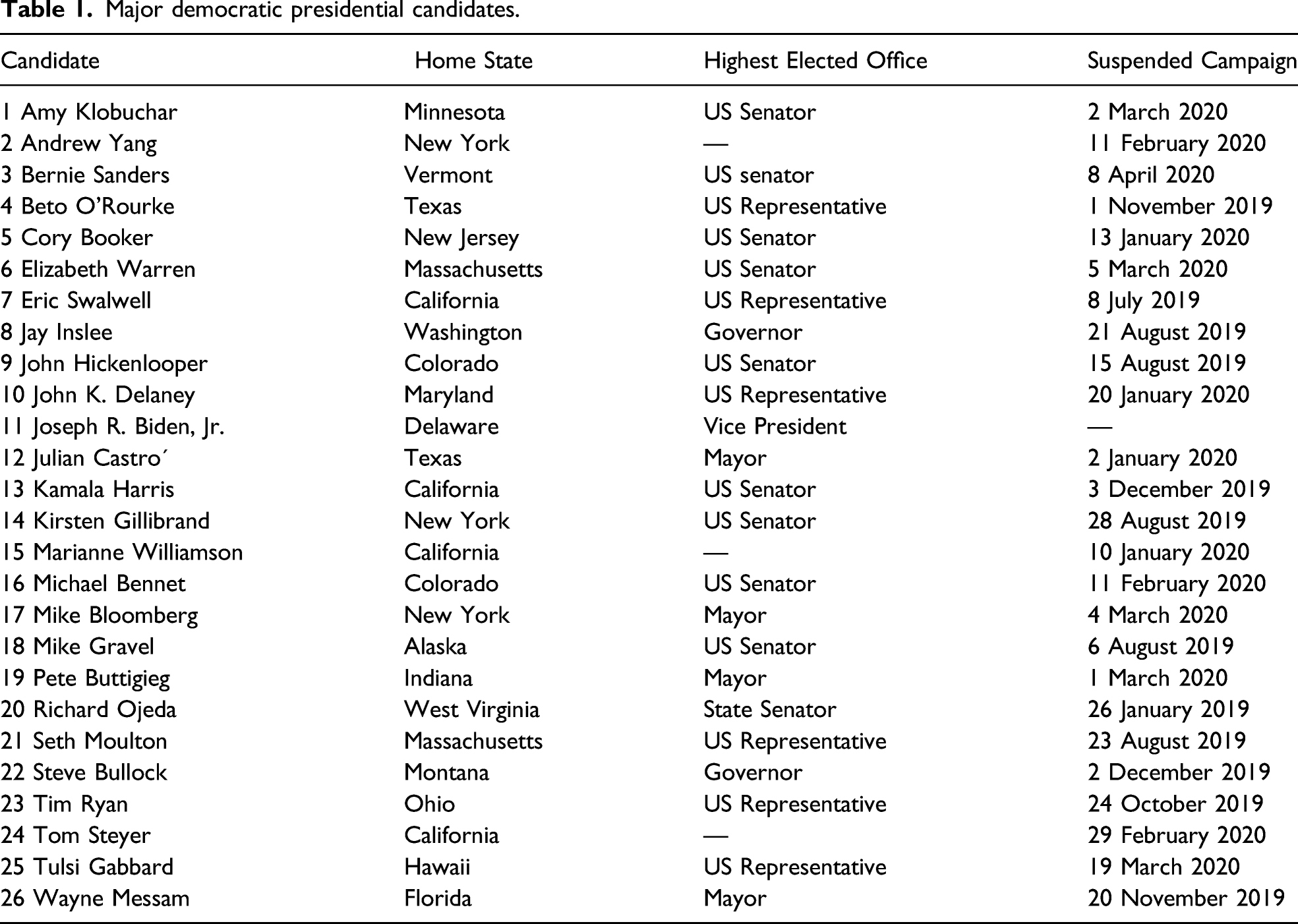
Candidates’ attrition pattern corresponds relatively closely to their campaigns’ ad expenditures on the Facebook platform. Figure 4 shows the monthly activity of candidates competing for the nomination and running Facebook ads. As indicated by the raised gray blocks, most purchased ads over a period of six months or longer between January 2019 and March 2020. Several candidates, such as eventual nominee Joe Biden and major contenders Pete Buttigieg and Michael Bloomberg, did not begin advertising on Facebook until several months into 2019. Just three candidates—Amy Klobuchar, Bernie Sanders, and Elizabeth Warren—purchased ads in each of the months included in our study. The advertising cycle began in January 2019 with 18 candidates and gradually increased to a mid-year peak of 24, before declining steadily to just six candidates publishing ads leading up to Super Tuesday in March 2020 (see the lower panel of Figure 4). Since many candidates were already elected officials, we exclude ads published prior to January 2019 to distinguish between the 2020 primary season and the 2018 midterm election season.

Figure 4.

The dataset contains information about 26 Democratic candidates, most of whom did not actively advertise for the entire period of observation (Jan 2019–March 2020).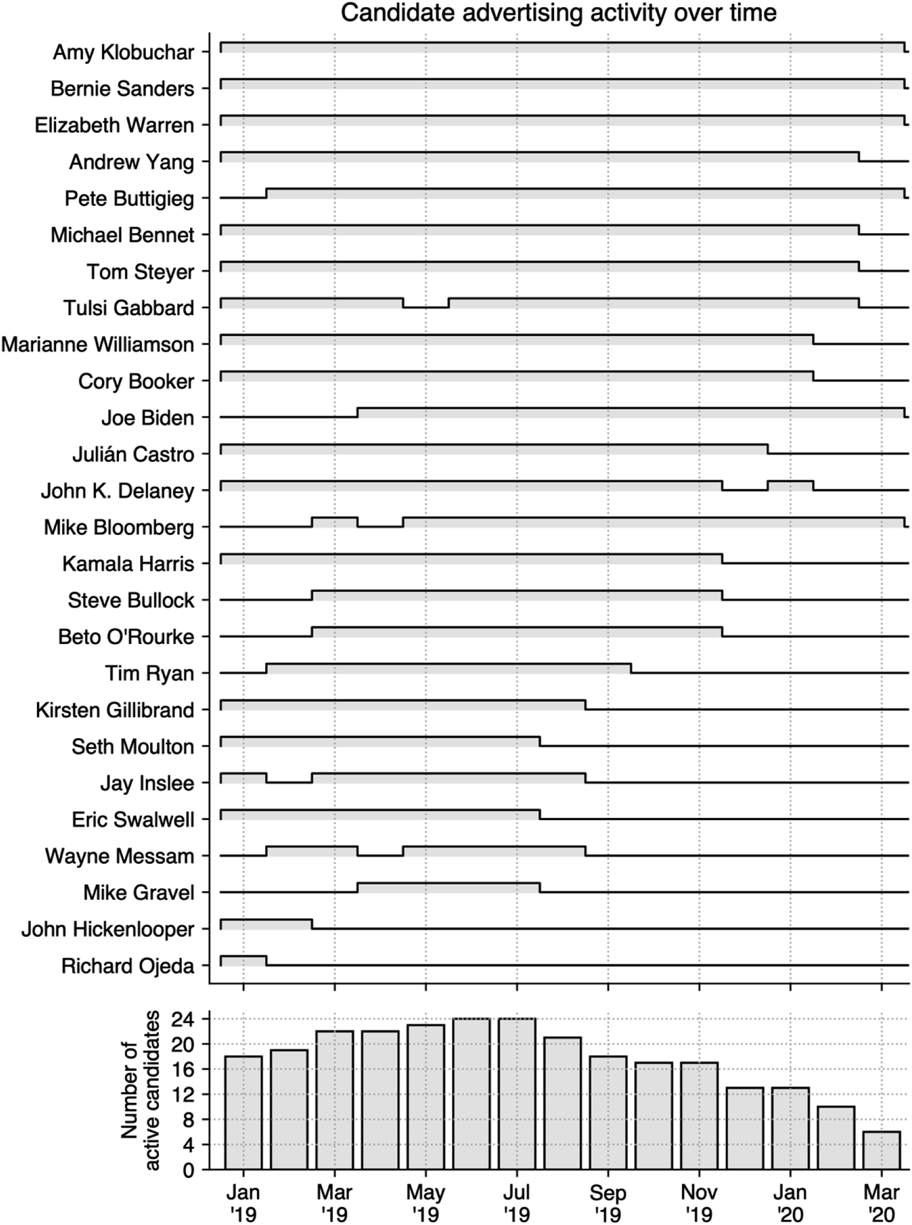

Ad spending varied widely across campaigns, with the majority spending $5 million or less. Figure 5 shows estimated spending on Facebook advertising for each campaign, as well as the total monthly spending for all candidates over time. While spending gradually increased over the course of the primary cycle, the large spikes in early 2020 can be attributed to wealthy candidates such as Michael Bloomberg. The Democratic nominee, Joe Biden, ranked 7th among the highest spending candidates.

Figure 5.

(A) Approximate Facebook ad expenditure among campaigns since January 2019 and (B) total spending per month for all campaigns.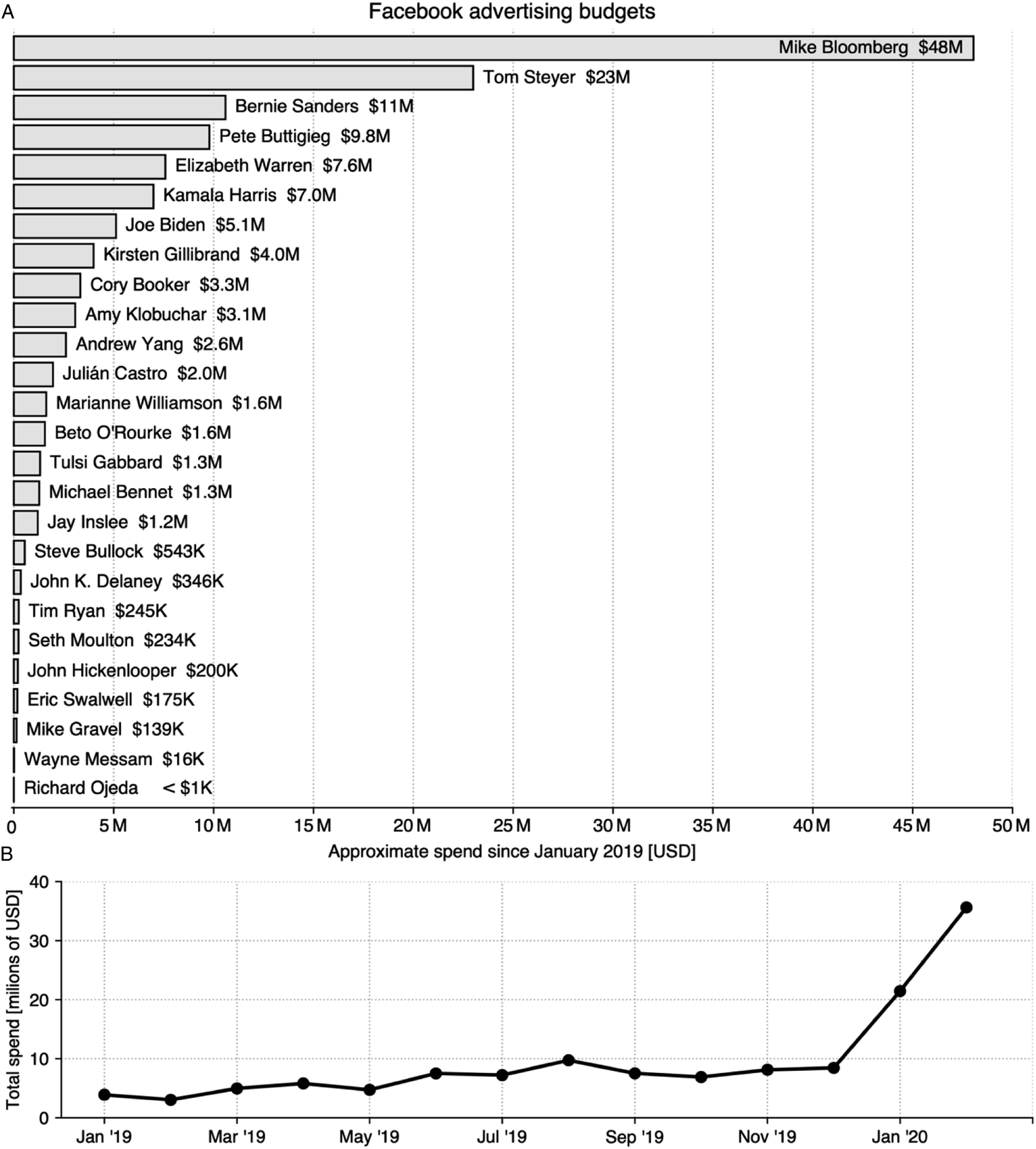

Throughout the invisible primary period, most candidates spent more on advertising per resident in their home state compared to outside of their home state, as presented in Figure 6. For many candidates, ad spending in home states was at least 20 times higher, particularly during the first half of the invisible primary. Candidates who dropped out of the primary in late 2019 also tended to spend disproportionately more in their home states in early 2019 than those who dropped out in early 2020.

Figure 6.

Comparison between ad spend in home state versus outside of home state. Most candidates spent more in ads per resident in their home states than outside of their home states and this behavior persists throughout the invisible primary period. John Hickenlooper, who advertised for two months, and Richard Ojeda, who advertised for one month, are excluded as outliers.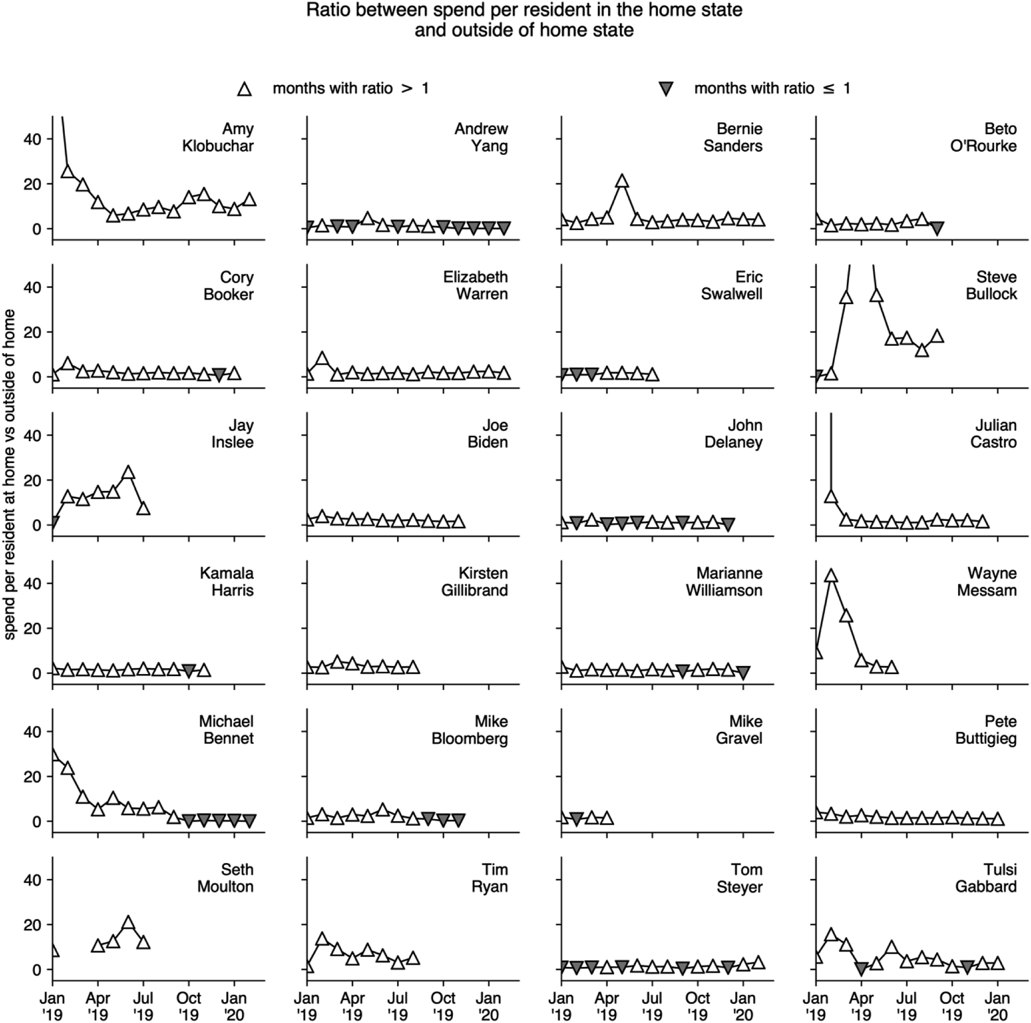

State Characteristics

Our analysis examines the extent to which candidates target voters in states with characteristics that correspond to our hypotheses. Table 2 provides a breakdown of binary state characteristics, including candidate home states, swing states, and states with early contests. We consider a candidate’s home to be the state in which he or she held an elected position or resided as of 1 January 2019, and we consider swing states to be those identified by poll aggregator FiveThirtyEight during the 2016 general election cycle (Silver, 2016).

Table 2.

State primary characteristics.

Candidate home state	AK, CA, CO, DE, FL, HI, IL, IN, MD, MA, MN, NJ, NY, OH, TX, VT, WA, WV
Swing state in 2016	AZ, CO, FL, GA, IA, ME, MI, MN, NV, NH, NC, OH, PA, UT, VA, WI
February primary	IA, NH, NV, SC
Super Tuesday primary	AL, AR, CA, CO, GA, MA, MN, NC, OK, TN, TX, UT, VT, VA
Caucus	AK, CO, HI, ID, IA, KS, ME, MN, NE, NV, ND, UT, WA, WY

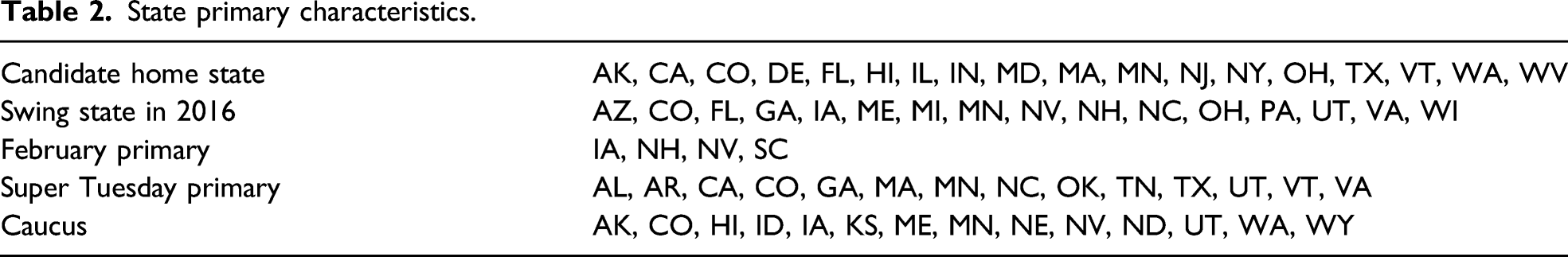
Of the four states that hold caucuses or primaries in February, Iowa and New Hampshire are considered key litmus tests for candidate viability. South Carolina’s primary at the end of February is also important to candidates because it is the first primary with a large block of black voters. On Super Tuesday, 14 states held primaries to allocate 1,600 delegates—the largest number on any single day of the season. Following Super Tuesday 2020, only five candidates remained: presumptive nominee Joe Biden, Elizabeth Warren, Michael Bloomberg, Tulsi Gabbard, and Bernie Sanders.

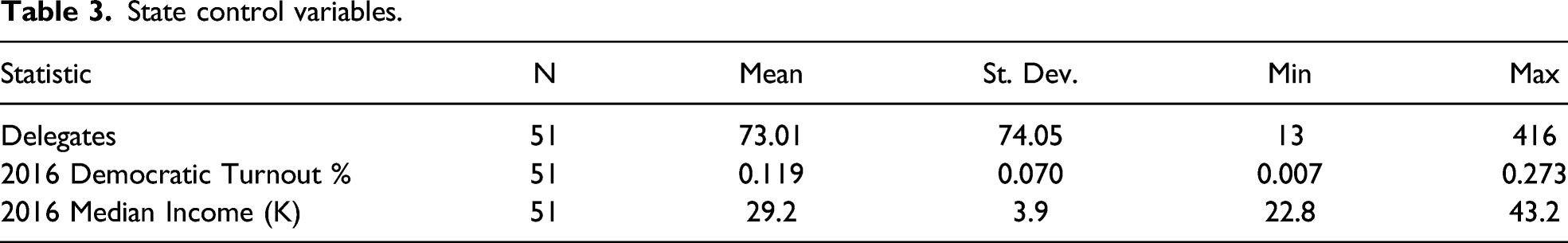
Our hypotheses consider three explicit state-level strategies—home states, swing states, and states with early primaries—which we expect to vary over time. We also consider whether campaigns have alternative motivations to target a particular state, such as contest type (caucus or primary), access to rich donors, potential for high fundraising yield, and overall number of delegates (Bartels, 1985; Brown Jr et al., 1995; Ridout et al., 2009). We include an indicator for states that hold caucuses rather than primaries in Table 2. In Table 3, we report descriptive statistics for 2016 median income in thousands, 2016 Democratic turnout as a proportion of the voting eligible population, and the number of delegates.

Table 3.

State control variables.

Statistic	N	Mean	St. Dev.	Min	Max
Delegates	51	73.01	74.05	13	416
2016 Democratic Turnout %	51	0.119	0.070	0.007	0.273
2016 Median Income (K)	51	29.2	3.9	22.8	43.2

Methodology

Consider a campaign i with a monthly budget to allocate to different states {1,...,S}. The number of observations for each month is equal to N_i × S, where N_i is the number of active campaigns i and S = 51, the US states plus the District of Columbia.

To construct our dependent variable, we draw on the approach of television advertisers. Television media buyers use a metric called gross ratings points (GRPs) to measure the reach of an individual ad (Fowler, Franz, and Ridout, 2018). An ad receives one GRP for each percentage point of the target audience reached by the ad’s airing. These GRPs can then be aggregated to express an advertiser’s total budget. We extend this approach to construct an aggregated measure of digital reach but with two changes to account for wide variation in campaign budgets and state populations. First, we express the campaign’s budget as a proportion. We use the budget proportion as our dependent variable rather than the dollar amount because it allows us to compare candidates whose budgets vary by orders of magnitude. Second, we normalize this proportion by each state’s population. The total amount of contributions that comes from a state is highly correlated with that state’s population regardless of the campaign’s leaning or strategy (Gimpel et al., 2006). In our data, the correlation between per state budgets and the state populations across all campaigns is on average ρ = 0.61. Normalizing by population allows us to compare how much value campaigns assign to voters living in states whose populations vary by orders of magnitude. We define Y_is as the population-normalized proportion of the advertising budget allocated to state s by campaign i. If a campaign spends money in direct proportion to the number of inhabitants, then Y_is = 1. When campaigns spend more or less than expected given a state’s population, then $Y_{i s} \neq 1$ .

Each state s has a set of characteristics taken into consideration by a campaign. The variable Home is a binary indicator with a value of 1 if s is the home state for campaign i. Swing indicates whether state s is considered a swing state, meaning it was not characterized by a clear preference toward Democratic or Republican candidates in recent elections. We include February primary and Super Tuesday primary to indicate whether state s holds an early caucus or primary.

To estimate the budget proportion, we fit the following baseline model using ordinary least squares: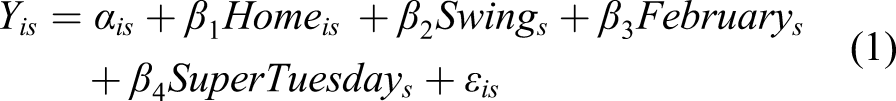

Y_{i s} = α_{i s} + β_{1} H o m e_{i s} + β_{2} S w i n g_{s} + β_{3} F e b r u a r y_{s} + β_{4} S u p e r T u e s d a y_{s} + ε_{i s}

(1)

The intercept is the ratio of state budget to state population. This value should be approximately one, reflecting our expectation that campaigns will spend more money in states with larger populations. The coefficients {β₁, β₂, β₃, β₄} are our quantities of interest. A coefficient greater than zero means that campaigns spent more to target the same share of residents in states with that characteristic.

Any effort to disentangle the dynamics of campaign behavior must contend with omitted variable bias. To address this, we add a set of control variables to our baseline model, including an indicator for states that conduct caucuses rather than primaries, the number of delegates, median household income, and Democratic turnout from the 2016 presidential election. Second, we specify alternative specifications with state fixed effects, which capture all unobservable factors that do not vary by state over time. Because we cannot include both state fixed effects and a full set of state-level variables, we use the fixed effects specifications to examine the estimates for key states and to investigate the robustness of our models. We also specify a separate model with candidate fixed effects to account for unobserved candidate characteristics that were fixed over the course of the primary. We use these effects to capture the influence of stable factors such as private wealth (Adkins and Dowdle, 2002), pre-existing political networks (Adkins and Dowdle, 2002; Hinckley and Green, 1996; Lewis-Beck and Rice, 1983), and social identities (Brown Jr et al., 1995).

Results

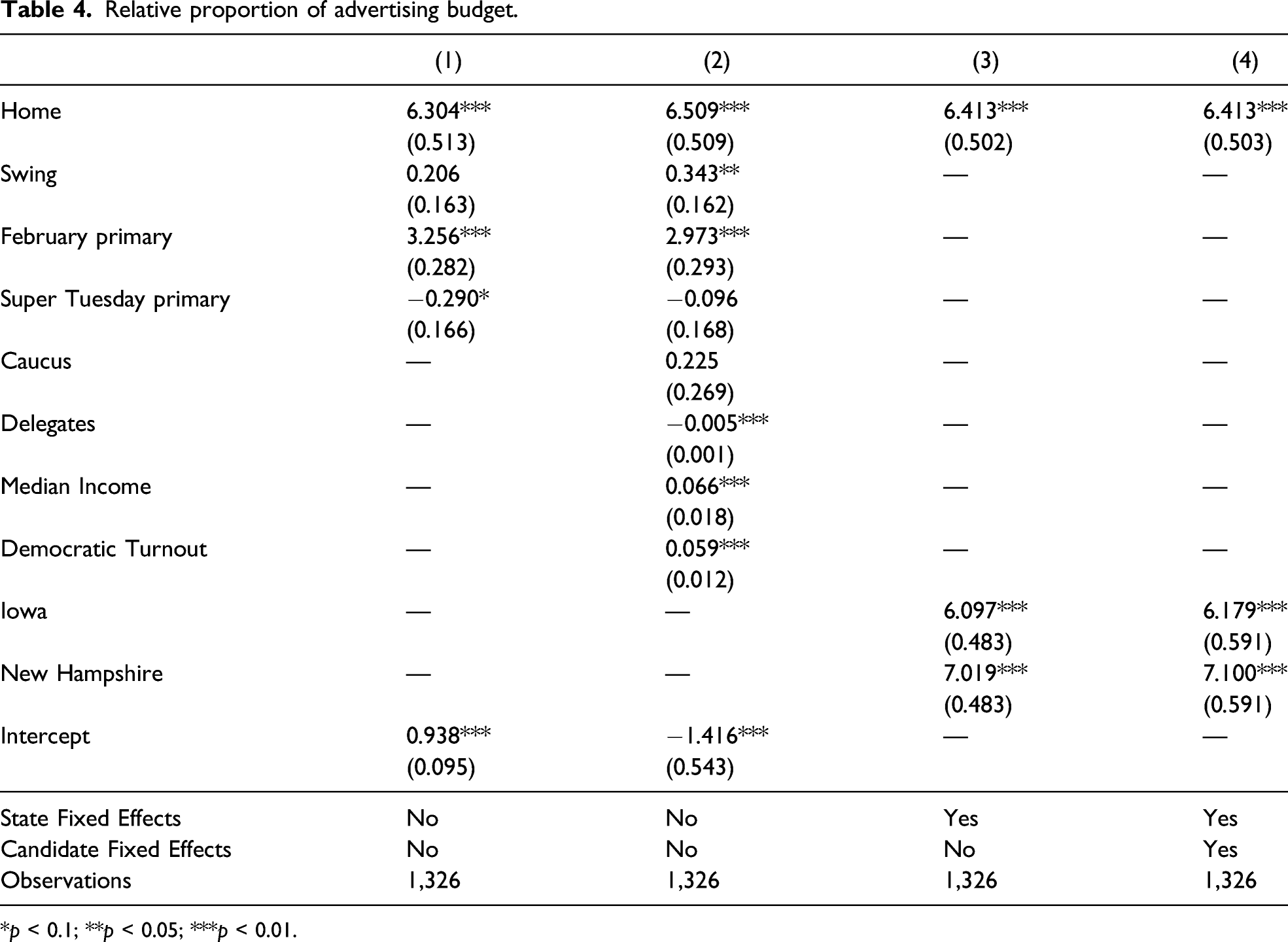
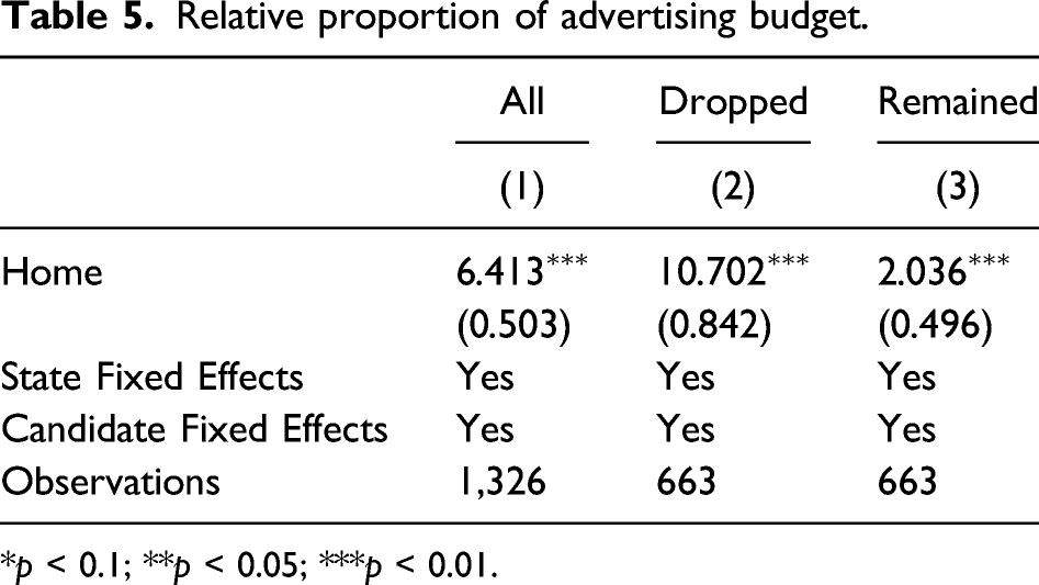
We report results for aggregate state-level spending in Table 4. We then report results from a series of independent monthly and weekly models to reflect the temporal changes.

Table 4.

Relative proportion of advertising budget.

	(1)	(2)	(3)	(4)
Home	6.304^***	6.509^***	6.413^***	6.413^***
	(0.513)	(0.509)	(0.502)	(0.503)
Swing	0.206	0.343^**	—	—
	(0.163)	(0.162)
February primary	3.256^***	2.973^***	—	—
	(0.282)	(0.293)
Super Tuesday primary	−0.290^*	−0.096	—	—
	(0.166)	(0.168)
Caucus	—	0.225	—	—
		(0.269)
Delegates	—	−0.005^***	—	—
		(0.001)
Median Income	—	0.066^***	—	—
		(0.018)
Democratic Turnout	—	0.059^***	—	—
		(0.012)
Iowa	—	—	6.097^***	6.179^***
			(0.483)	(0.591)
New Hampshire	—	—	7.019^***	7.100^***
			(0.483)	(0.591)
Intercept	0.938^***	−1.416^***	—	—
	(0.095)	(0.543)
State Fixed Effects	No	No	Yes	Yes
Candidate Fixed Effects	No	No	No	Yes
Observations	1,326	1,326	1,326	1,326

^*p < 0.1; ^**p < 0.05; ^***p < 0.01.

Aggregate Model

Our baseline model includes indicators for home states, swing states, and states with primaries in February and on Super Tuesday (Table 4, Column 1). The Intercept is slightly smaller than one, suggesting that on average, campaigns spend in rough proportion to states’ populations.

Campaigns Spend Considerably More in Home States

Given the large magnitude and statistical significance of the Home coefficient (Column 1 of Table 4), we conclude that campaigns spend significantly more on ads in candidates’ home states, in line with our hypothesis (H1). A hypothetical candidate whose home state is neither a swing state nor early in the primary calendar would spend a fraction of their budget per capita that is 7.2 times higher than in another non-swing, late-primary state (6.304 + 0.938 ≈ 7.2). Home also exceeds the estimated budget allocations for swing states and states with early primaries.

The magnitude and significance of the home state effect—more than six times the average budget allocation per resident—is robust across model specifications that include controls, state fixed effects, and candidate fixed effects. We report estimates for the baseline model with control variables in Column 2. The indicator for caucuses is not significant, while the number of delegates, median income, and Democratic turnout are highly significant but small in magnitude.³ Since our dependent variable accounts for the size of a state’s population, and the number of delegates is closely related to the population, we are not surprised that Delegates is near zero. The positive coefficients for turnout and median income suggest that the potential to tap high-income donors and mobilize Democratic voters exerts some small influence on campaigns’ strategies.

One possible explanation for home state spending is that it is driven by candidate status. To test this, we estimated the home state effect separately for each candidate using monthly ad expenditures. Figure 7 shows each candidate’s home state effect, grouped by the highest office held by the time of the invisible primary. Of the 25 candidates, all but three allocated up to 10 times the monthly budget to their home states. While a handful of candidates spent much more than their peers, the estimated monthly budget allocations are similar regardless of office held. The three candidates who had not held any office are among the minority for whom the home state effect is not significant. This may suggest that home states presented less of an opportunity for candidates without pre-existing political networks. We further note that the two governors are among the candidates with the highest home effect sizes. At the same time, the home state coefficient for Joe Biden, a former Vice President, is significant but small. We therefore conclude that the home state effect size is not explained by candidate status.

Figure 7.

The home state focus is not only the domain of candidates who held low or no offices in the past, that is, those who need the recognition the most. We excluded Richard Ojeda, who met our criteria for a major candidate but advertised for only one month.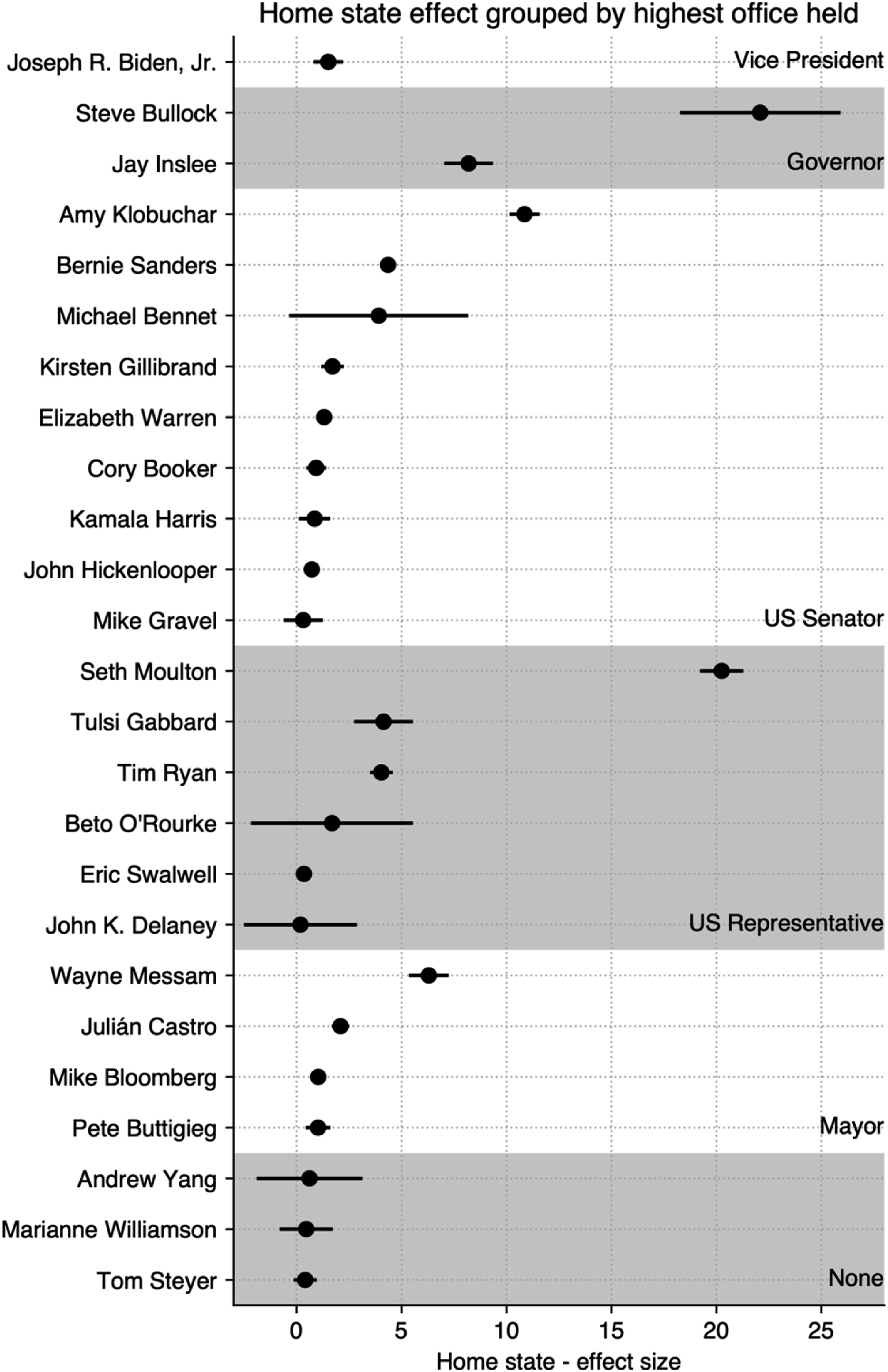

Campaigns Target Swing states, but Less So Than Home States

The positive and statistically significant value of the Swing state coefficient in Column 2 of Table 4 supports our second hypothesis, that campaigns target voters in swing states in a manner disproportionate to their populations. The coefficient for Swing is positive but not significant in our baseline model. For both the baseline and model with controls, the low magnitude of the coefficient (β₂ = 0.343) suggests that battleground status alone is not a strong predictor of ad spending during the primary cycle. This can be explained by the fact that swing states are more critical for the general election than the primary election. Swing states may warrant more digital advertising during the general election, after the major party nominees have been determined.

Earliest Primaries More Consequential than Super Tuesday

We find strong support for our third hypothesis that campaigns target voters in states with early primaries. We considered two types of calendar effects: (1) February primaries where the number of delegates is small but signaling candidate viability is important; and (2) Super Tuesday primaries that generate momentum by allocating a large number of delegates relatively early in the cycle.

The positive, significant coefficient for February Primary and negative, null coefficient for Super Tuesday Primary suggest that campaigns embraced the first strategy—targeting the first few primaries in Iowa, New Hampshire, Nevada, and South Carolina. Campaigns allocated roughly three times the per capita budget to target voters in these states. We find weak evidence that campaigns spent less than average (β₃ = −0.29) per capita in Super Tuesday states.

States with February primaries were targeted heavily, but still less so than candidates’ home states. In Columns 3 and 4 of Table 4, we estimate Home with state and candidate fixed effects. We are unable to include additional variables in these models due to perfect or multicollinearity.⁴ We report the fixed effects for Iowa and New Hampshire, the first two contests in February. The large magnitudes of these fixed effects, 6.1 for Iowa and 7.0 for New Hampshire, provide further evidence that campaigns prioritized the earliest primaries.

Temporal Model

To examine our final hypothesis, that campaigns’ targeting strategies shift away from the home states and toward early primary states over time, we fit the model to each month of data independently. Our results provide evidence that campaigns alter their strategies over time—heavily targeting home states early in the primary cycle and shifting to early primary states and swing states as the first primaries and caucuses approach in February. Further, we show that advertising in Super Tuesday states and swing states remains flat throughout the duration of the time period we study. In our temporal analysis, we find that the Home effect is robust to the inclusion of state fixed effects, candidate fixed effects, and state-level control variables.⁵

Campaigns Target Home States During First Phase of Calendar

It is instructive to look at the 14-month period in two phases: the first from January through July 2019, and the second from August 2019 through February 2020. Phase I is characterized by heavy to moderate spending in home states and moderate spending in February primary states. Panel A of Figure 8 shows that political advertising is the most intense in the home state of each candidate at the beginning of 2019: more than a year before the first race, campaigns spent nine times the average budget proportion per capita in these states. During this phase, spending in swing states (other than February primary states) and Super Tuesday primary states remained constant, with coefficients at or near zero over the seven-month period.

Figure 8.

In January 2019, campaigns spent as much as 9 times more in their home states than expected given their population, but the importance of home states drops over time. In contrast, states with primaries in February see increasing spends over time, as do, to a lesser extent, the swing states.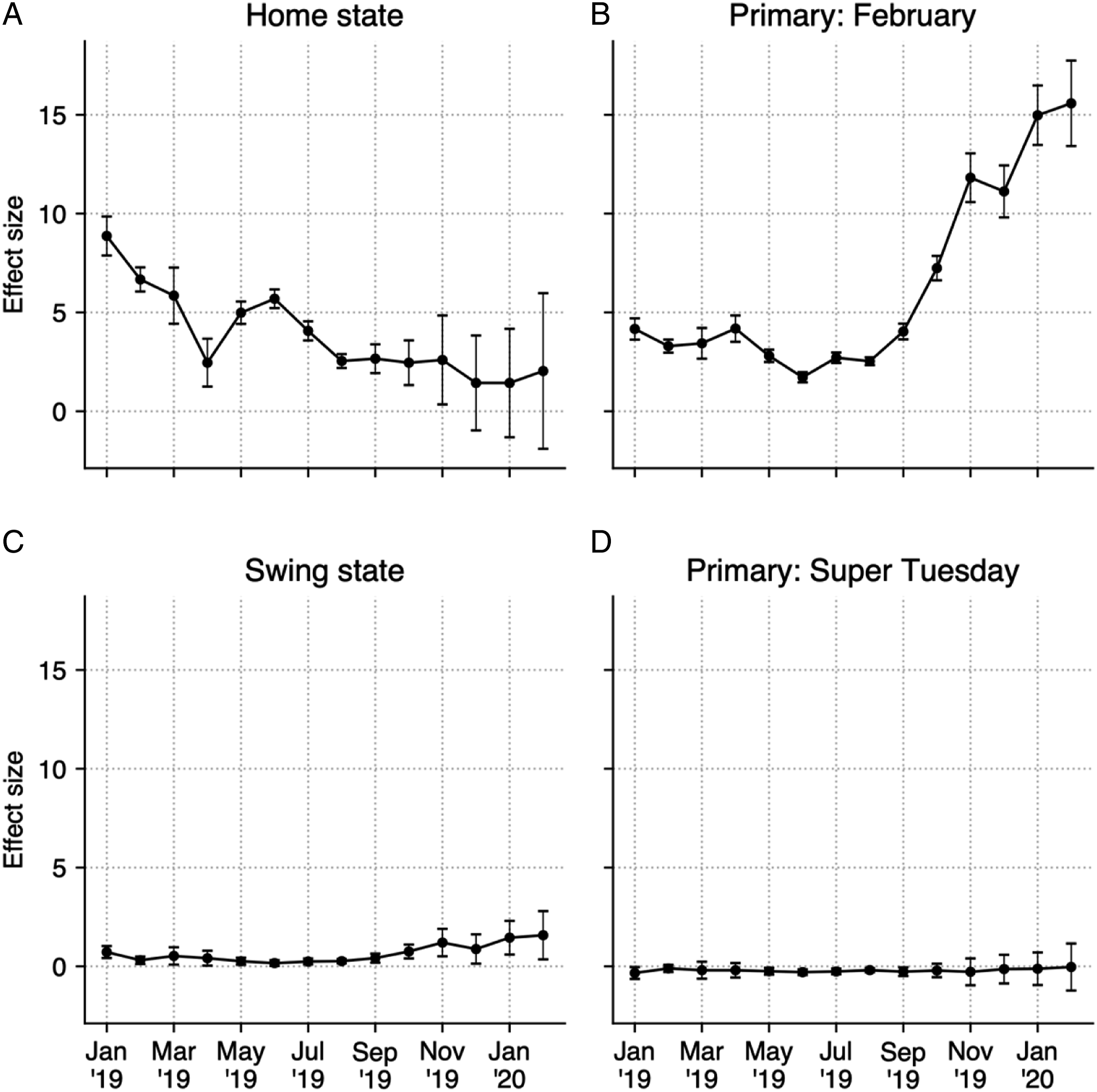

The overall pattern in the Home coefficient during Phase I suggests that campaigns leveraged digital advertising to qualify for the Democratic debates. Following a large boost in January 2019, spending declines until May 2019, when spending rises to a second peak in June 2019. This second peak corresponds to a push by campaigns to meet polling and fundraising thresholds for the first debates, which were held on June 26 and 27, 2019. The Democratic National Committee (DNC) required that candidates, “register 1% or more support in three polls released between 1 January 2019, and 14 days prior” to the first debate (Democratic National Committee, 2019). Candidates also required “(1) 65,000 unique donors; and (2) a minimum of 200 unique donors per state in at least 20 US. states.” Since the unique donor threshold is much higher than the individual state donor minimum, campaigns would have an incentive to target their home states to attract the number of donors needed. In addition to debate qualification thresholds, the historically large field of major candidates impacted campaigns’ incentives. The DNC set a cap of 20 candidates for the first set of debates. Facing a crowded field of 26 major candidates, campaigns would have sought to meet and even exceed the qualification thresholds to ensure debate participation. Failure to meet debate thresholds may explain why, after the first debate, a substantial number of candidates stopped publishing advertisements on Facebook.

Given the declines in spending that occurred after the debates, we consider the extent to which our results are driven by candidate attrition over time. All but two of the 26 major candidates in our sample were active on the platform during the first phase of our temporal analysis (through July 2019). During this first phase, where home state spending is most pronounced, there was minimal change to the composition of candidates. During the second phase, approximately half of the candidates stopped advertising on the Facebook platform. Those who continued advertising through the end of the year included a mix of established candidates such as Bernie Sanders and Joe Biden, long-shot candidates such as Andrew Yang and Pete Buttigieg, and candidates that fall somewhere between, such as Elizabeth Warren.

We estimated the home state effect for two candidate groups: those who dropped in late 2019, and those who remained through early 2020. These results, estimated using the data between January 2019 and December 2019, are shown in Table 5. We find that the focus on home states that is most prevalent in Phase I is not merely an artifact created by candidates who dropped out of the race early—both groups allocated significantly more money to their home states. However, there are some key differences between the groups. First, the home state effect for the candidates who remained is significant but has a much lower magnitude (β = 2.0) than that of the candidates who dropped (β = 10.7). Second, the groups exhibit differences in timing. Figure 9 shows the home state effect size for each month: stars indicate candidates that dropped out of the race in late 2019, while points indicate candidates that remained through early 2020. The boost in home state spending that we observe in June 2019, shortly before the first debate, is much more pronounced for the candidates who subsequently dropped out of the race. The sharper peak suggests that weaker candidates were particularly focused on meeting the threshold for debate participation. Stronger candidates, who likely met the debate threshold easily, still targeted their home states, but to a lesser extent.

Table 5.

Relative proportion of advertising budget.

	All	Dropped	Remained
	(1)	(2)	(3)
Home	6.413^∗∗∗	10.702^∗∗∗	2.036^∗∗∗
	(0.503)	(0.842)	(0.496)
State Fixed Effects	Yes	Yes	Yes
Candidate Fixed Effects	Yes	Yes	Yes
Observations	1,326	663	663

^*p < 0.1; ^**p < 0.05; ^***p < 0.01.

Figure 9.

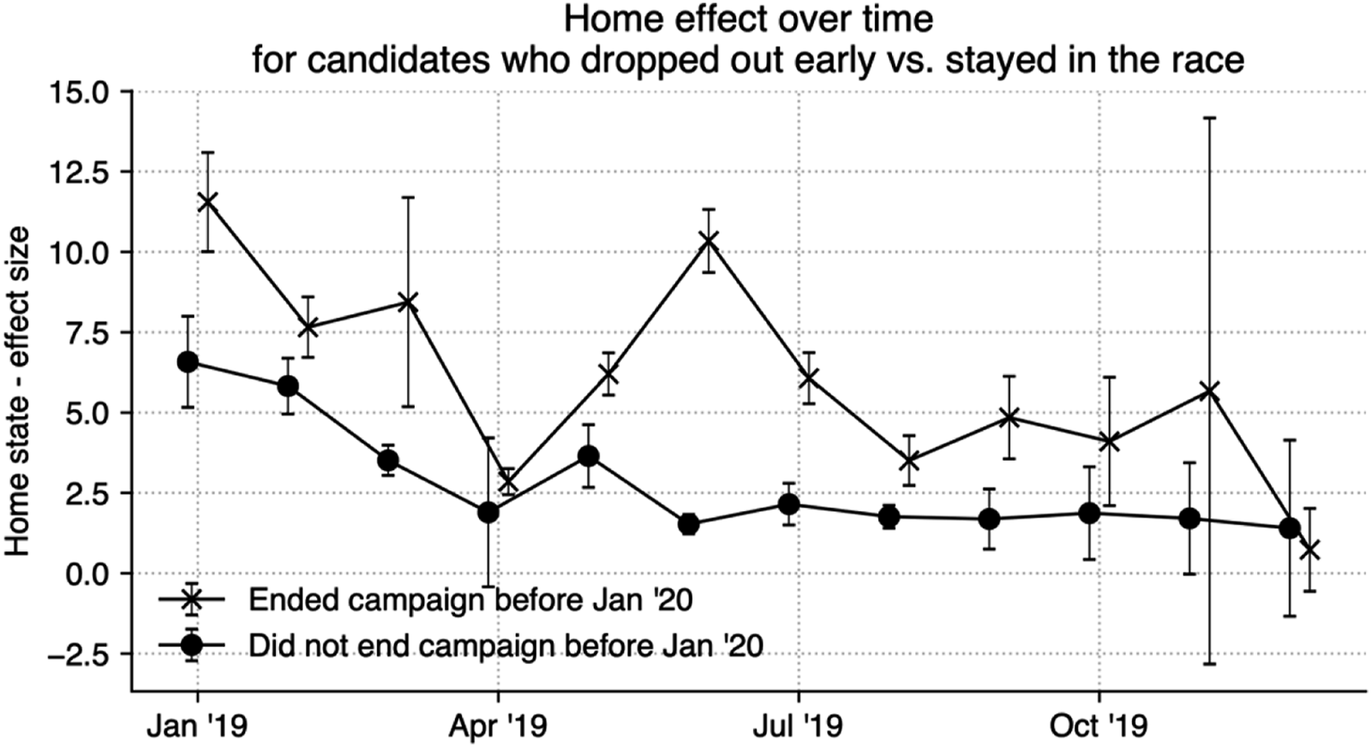
The home state effect is driven both by candidates who ended their campaigns before January 2020 as well as those who stayed in the race beyond that point, although the effect is stronger for the former group.

February Primary States Targeted Heavily In Second Phase

During Phase II of the cycle, between August 2019 and March 2020, campaigns spent heavily in February primary states (Figure 8B), a majority of which are also swing states, and spent slightly more in other swing states (Figure 8C). Home state spending remained constant at a quarter of its Phase I peak, and spending in Super Tuesday states remained constant with coefficients at or near zero. By the end of Phase II, campaigns spent up to 16 times the proportionate baseline in states with the earliest primaries. This is three times more advertising than the February primary state baseline in June 2019, the peak at the end of Phase I.

To examine these effects more closely, we focus on the weeks leading up to the first primaries in February and March. During this time period, the number of candidates decreased from 13 to 6. As a result, these estimates exhibit higher variance than those from earlier in the primary. Figure 10A shows that states with a February primary received 15 to 18 times more spending than expected given their populations, up to the first week of February. After the Iowa caucuses, the focus switched to the remaining February states and as campaigns stop showing ads in Iowa, the effect size nearly disappears by the end of February. In contrast, Figure 10B shows that the Super Tuesday states do not receive significantly more spending until the last week of February and first week of March, indicating that the campaigns focus spending on locations that are immediately next in the primary calendar.

Figure 10.

(A) The effect size of a primary in February is high through the first weeks of 2020. After each actual primary event, the effect size drops and nearly disappears by the last week of February/first week of March. (B) On the other hand, the states that hold their primaries on Super Tuesday only see increased advertising in the last 2 weeks leading up to the date.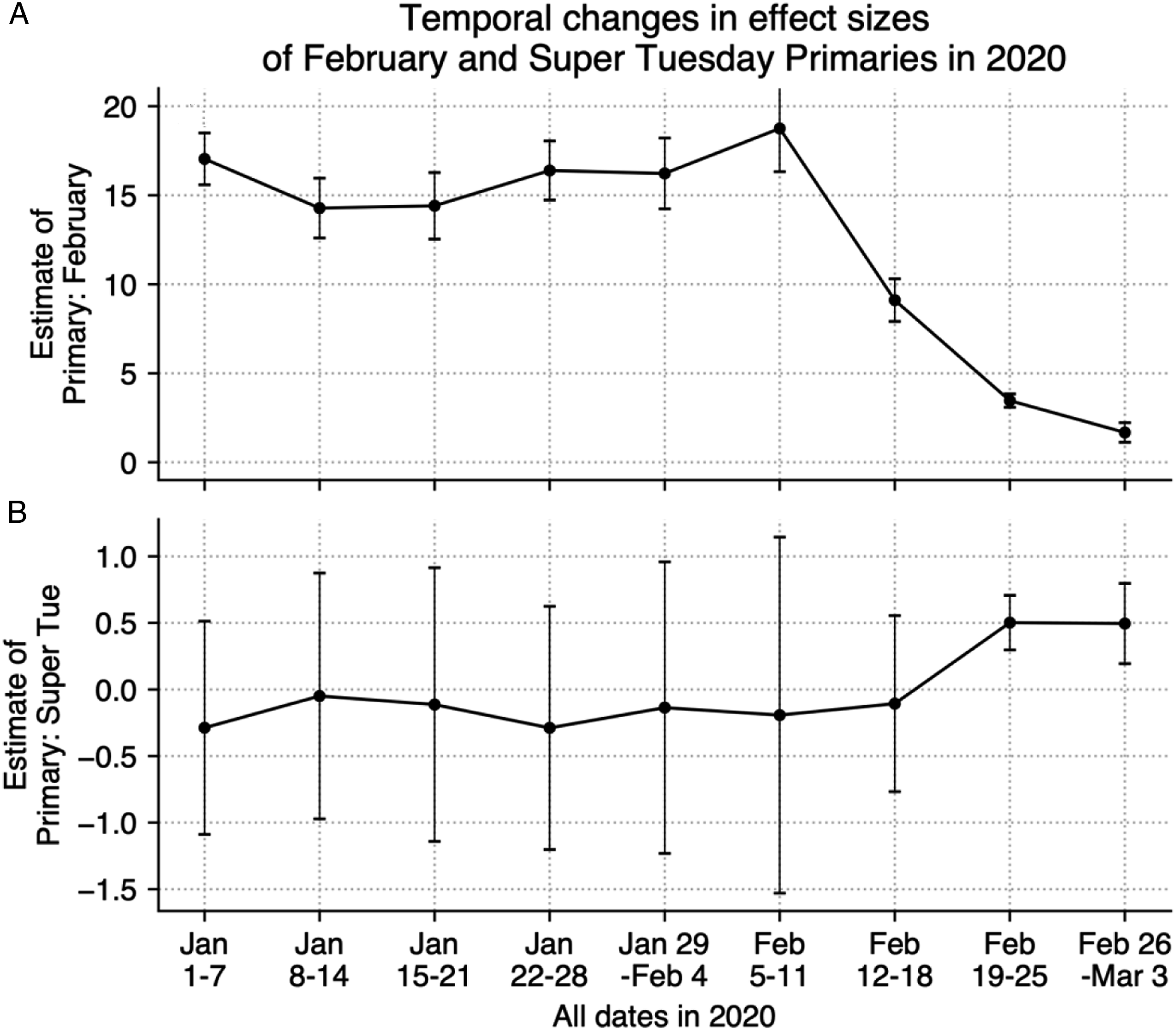

Discussion

As digital advertising has grown as a proportion of campaign spending, television and other forms such as radio and direct mail have declined. Is digital advertising simply displacing other forms of advertising or supplementing them? Our findings suggest that digital ads may both displace some forms of advertising and present new strategic opportunities for campaigns.

Fundraising is most critical in the earliest stages of the invisible primary (Adkins and Dowdle, 2002). In a detailed accounting of campaigns and contributors from the 1988 and 1992 presidential elections, Brown and colleagues show that candidates use direct mail primarily to solicit contributions from past donors in their home states, a finding echoed by later analyses of direct mail received by a national sample of voters during the 2004 presidential election (Brown Jr et al., 1995; Hassell and Monson, 2014). Our analysis, which shows that digital ad spending in home states follows a similar pattern, suggests that digital ads may be the new direct mail. However, in contrast to earlier studies showing that direct mail expenditures are tied to existing networks, we find that candidates spend more in their home states regardless of the size of their political network. Home states are valuable for both connecting to and expanding a candidate’s network of supporters, particularly through small-dollar donations. During the 2008 primary season, Barack Obama exceeded fundraising expectations by raising nearly $30 million from individuals donating $100 or less (Luo, 2008). Donald Trump’s 2020 re-election campaign fully embraced this strategy, spending heavily on digital advertising and receiving 725,000 small-dollar donations (Karni and Haberman, 2019).

Broadcast television remains the largest and most expensive advertising expenditure for campaigns. The vast array of television channels and specialized programming have allowed campaigns to engage in sophisticated targeting of viewers (Edsall, 2012; Ridout, Franz, Goldstein, and Feltus, 2012). Targeting options offered by digital platforms surpass these programming-based mechanisms, allowing campaigns to target largely unknown individuals on the basis of demographic characteristics, political views, and precisely defined interests. Digital platforms may therefore reduce entry barriers for long-shot candidates by providing them with an alternative to broadcast television advertising, which is generally accessible to only the most well-resourced candidates. Our findings show that candidates with widely varying budgets used digital platforms to strategically target supporters and voters.

To compare digital advertising strategies to broadcast strategies, we examined estimated spending on television advertisements during the 2008 and 2012 presidential primary cycle (Fowler et al., 2017; Goldstein et al., 2011). Examining only major candidates and ads purchased by campaigns rather than parties or committees, we find that campaigns have not used television advertisements to target voters in candidates’ home states. During the 2008 primary cycle, just four of the 13 major campaigns advertised in television markets where voters from the candidate’s home state comprised the core audience (see Figure 11). However, virtually no home state targeting occurred early in the primary cycle. Notably, Barack Obama, who won the nomination, spent more on television advertising than any other candidate ($51.3 M) but did not allocate any of this budget to target voters in his home state of Illinois. During the 2012 cycle, just one major candidate, Mitt Romney, advertised in his home state of Massachusetts.

Figure 11.

During the 2008 presidential primary cycle, just four candidates purchased television airtime in their home states, all in the weeks leading up to the first primaries and caucuses in February. The absence of early cycle spending on TV ads suggests that long-shot campaigns may be using low-cost digital ads to compete with more established candidates.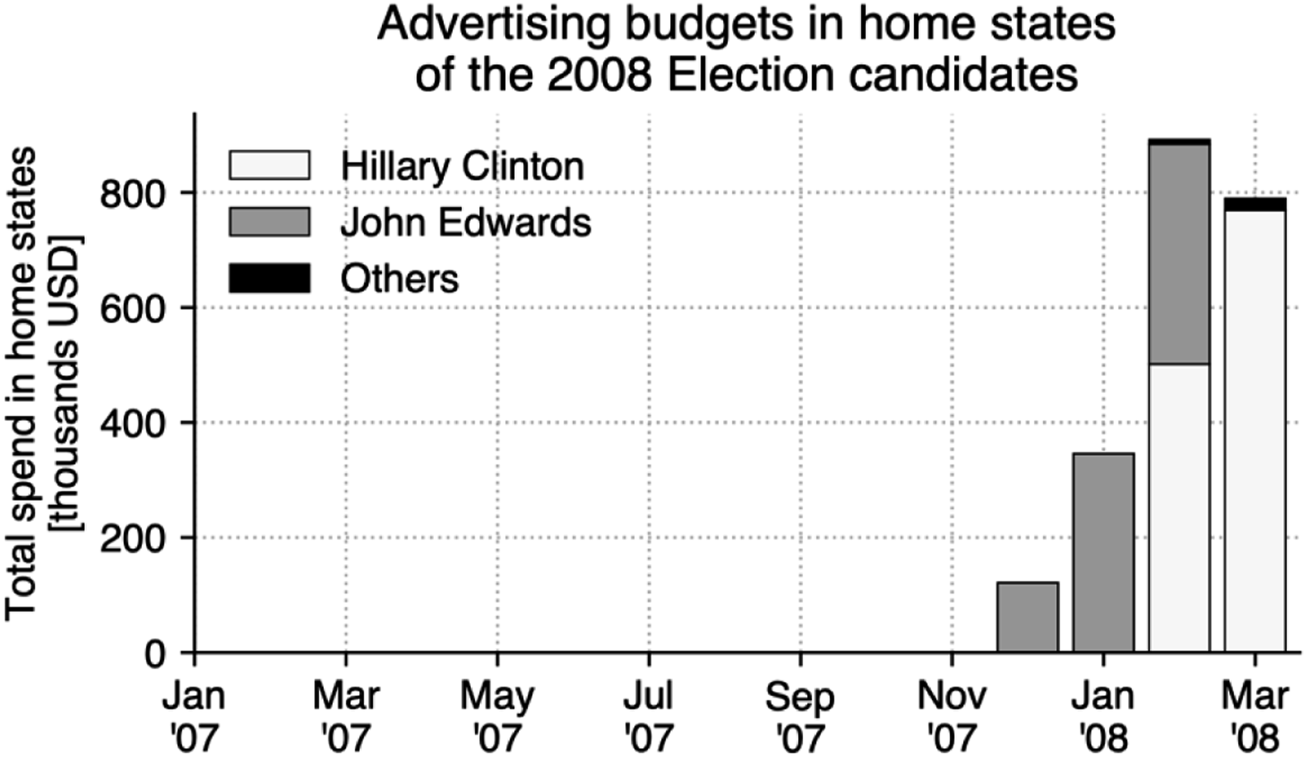

Comparisons between digital and television spending face important limitations. Broadcast television markets are organized into geographic units known as designated market areas (DMAs), which span multiple states and make it impossible to perfectly capture state-level spending. Further, although campaigns spend the vast majority of their advertising dollars with local broadcast stations, they may also purchase airtime from national or local cable networks, which utilize different geographic units. Campaigns often purchase airtime several months in advance in order to secure the lowest rates and avoid being locked out of prime airtime by competing advertisers (Fowler et al., 2018). This may explain why television spending is more concentrated in the weeks leading up to the first caucuses and primaries, as campaigns prioritize encouraging voters to turn out on election day. Even with the limited utility of comparing digital and television media spending, the absence of early cycle TV advertising suggests that digital media has ushered in a set of new and lower cost opportunities for campaigns to expand their reach.

Digital platforms are believed by some to disrupt the democratic process and drive political polarization. To maximize the number of ads shown and clicked, Facebook aims to display content it believes to be relevant, at the expense of apparently less germane material. Showing ads that the users do not already agree with might cause cognitive dissonance, drive the users off the platform and result in “antigrowth” (Horwitz and Seetharaman, 2020). This approach—when applied in the political context—can lead to negative societal effects. People who are algorithmically prevented from seeing a different point of view will eventually have a reduced pool of information when making their choices at the polling station.

On the other hand, digital platforms may improve democratic governance by increasing candidates’ access to primary contests. During the 2020 primary cycle, an unprecedented number of Democratic candidates utilized digital media in addition to other strategies to remain competitive. Since candidates can reach large numbers of voters with relatively small budgets, future primary cycles may be characterized by a competitive field that takes much longer to narrow than in the past. Further, candidates who lose the nomination may still exert influence by participating in debates and shaping other candidates’ platforms. Understanding the role of digital advertising in primary elections requires not only a comprehensive picture of how digital platforms are operated and governed, but also how they are used both by those who run the ads and those who consume them.

Footnotes

Acknowledgments

We thank Caitlin Chamberlain for superb research assistance, and Michael Bailey, Jonathan Ladd, David Lazer, Ryan Harrison, and participants of the 2019 Politics and Computational Social Science Conference at Georgetown University for helpful feedback. Piotr thanks Alan Mislove for continued support.

Declaration of Conflicting Interests

The author(s) declared no potential conflicts of interest with respect to the research, authorship, and/or publication of this article.

Funding

The author(s) received no financial support for the research, authorship, and/or publication of this article.

ORCID iD

NaLette M Brodnax

Notes

References

Adkins

R. E.

Dowdle

A. J.

2001. “How Important Are Iowa and New Hampshire to Winning Post-Reform Presidential Nominations?” Political Research Quarterly 54 2: 431‐444.

Adkins

R. E.

Dowdle

A. J.

2002. “The Money Primary: What Influences the Outcome of Pre-Primary Presidential Nomination Fundraising?” Presidential Studies Quarterly 32 2: 256‐275.

Aldrich

2009. “The Invisible Primary and Its Effects on Democratic Choice.” PS: Political Science and Politics 42 1: 33‐38.

Aldrich

J. H.

1980. Before the Convention: Strategies and Choices in Presidential Nomination Campaigns. University of Chicago Press.

Ali

Sapiezynski

Korolova

Mislove

Rieke

2021. “Ad Delivery Algorithms: The Hidden Arbiters of Political Messaging.” In ACM International Conference on Web Search And Data Mining’21 13‐21. New York, NY, USA: Association for Computing Machinery.

Almukhtar

Martin

Stevens

2019. February 2020 Presidential Primary Election Calendar. https://www.nytimes.com/interactive/2019/us/elections/2020-presidential-electioncalendar.html?rref=collection%2Fnewseventcollection%2F2020-election.

Bartels

L. M

. 1985. “Resource Allocation in a Presidential Campaign.” The Journal of Politics 47 3: 928‐936.

Bartels

L. M.

1988. Presidential Primaries and the Dynamics of Public Choice. Princeton University Press.

Brown

C. W.

Jr Powell

L. W.

Wilcox

1995. Serious Money: Fundraising and Contributing in Presidential Nomination Campaigns. Cambridge University Press.

10.

Cassino

2017. The Final Analysis: What Happened to Political Advertising in 2016 (And Forever). Borrell Associates.

11.

Center for Responsive Politics . 2020. Joe Biden – Online Ad Spending. https://www.opensecrets.org/2020-presidential-race/joe-biden/online-ad-spending.

12.

Christenson

D. P.

Smidt

C. D.

Panagopoulos

. 2014. “Deus ex Machina.” Political Research Quarterly 67, 1: 108‐122.

13.

Cohen

Karol

Noel

Zaller

2008. The Party Decides: Presidential Nominations Before and After Reform. University of Chicago Press.

14.

Democratic National Committee . 2019. DNC Announces Details for the First Two Presidential Primary Debates. https://democrats.org/news/dnc-announces-details-for-the-firsttwo-presidential-primary-debates/.

15.

Dowdle

A. J.

Adkins

R. E.

Steger

W. P.

2009. “The Viability Primary.” Political Research Quarterly 62 1: 77‐91.

16.

Edsall

T. B.

2012. Let the Nanotargeting Begin. https://campaignstops.blogs.nytimes.com/2012/04/15/let-the-nanotargeting-begin/.

17.

Erdody

Political Campaigns Boost Investment In Social Media Ads, 2018, https://www.ibj.com/articles/70545-political-campaigns-boost-investment-in-social-media-ads.

18.

Facebook . Facebook Ad Library, 2019, https://www.facebook.com/ads/library/.

19.

Fowler

E. F.

Franz

M. M.

Ridout

T. N.

. 2017. Presidential Political Advertising in the 2012 Cycle. Version 1.0 [dataset] Middletown, CT. The Wesleyan Media Project, Department of Government at Wesleyan University.

20.

Fowler

E. F.

Franz

M. M.

Ridout

T. N.

2018. Political Advertising in the United States. New York: Routledge.

21.

Gimpel

J. G.

Lee

F. E.

Kaminski

2006. “The Political Geography of Campaign Contributions in American Politics.” The Journal of Politics 68 3: 626‐639.

22.

Gimpel

J. G.

Kaufmann

K. M.

Pearson-Merkowitz

. Battleground States versus Blackout States: The Behavioral Implications of Modern Presidential Campaigns. Journal of Politics 2007; 69(3): 786–797.

23.

Goff

M. J.

2004. The Money Primary: The New Politics of the Early Presidential Nomination Process. Rowman and Littlefield Publishers.

24.

Goldstein

Niebler

Neilheisel

Holleque

2011. Presidential, Congressional, and Gubernatorial Advertising, 2008. Madison, WI: The University of Wisconsin Advertising Project, the Department of Political Science at the University of Wisconsin-Madison.

25.

Grush

J. E.

1980. “Impact of Candidate Expenditures, Regionality, And Prior Outcomes On The 1976 Democratic Presidential Primaries.” Journal of Personality and Social Psychology 38 2: 337‐347.

26.

Gurian

P.-H.

1986. “Resource Allocation Strategies in Presidential Nomination Campaigns.” American Journal of Political Science 30 4: 802‐821.

27.

Haenschen

Jennings

2019. “Mobilizing Millennial Voters with Targeted Internet Advertisements: A Field Experiment.” Political Communication 36 3: 357‐375.

28.

Hassell

H. J. G.

Monson

J. Q.

2014. “Campaign Targets and Messages in Direct Mail Fundraising.” Political Behavior 36: 359‐376.

29.

Hinckley

K. A.

Green

J. C.

1996. “Fund-Raising in Presidential Nomination Campaigns: The Primary Lessons of 1988.” Political Research Quarterly 49 4: 693‐718.

30.

Hirano

Lenz

G. S.

Pinkovskiy

Snyder

J. M.

2015. “Voter Learning in State Primary Elections.” American Journal of Political Science 59 1: 91‐108.

31.

Horwitz

Seetharaman

. Facebook Executives Shut Down Efforts to Make the Site Less Divisive, 2020, https://www.wsj.com/articles/facebook-knows-it-encourages-division-top-executives-nixed-solutions-11590507499?mod=djemalertNEWS.

32.

Karni

Haberman

. Trump and R.N.C Raised $105 Million in 2nd Quarter, a Sign He Will Have Far More Money Than in 2016, 2019, https://www.nytimes.com/2019/07/02/us/politics/trump-fundraising.html.

33.

Knight

Schiff

2010. “Momentum and Social Learning in Presidential Primaries.” Journal of Political Economy 118 6: 1110‐1150.

34.

Kreiss

Lawrence

R. G.

McGregor

S. C.

2018. “In Their Own Words: Political Practitioner Accounts of Candidates, Audiences, Affordances, Genres, and Timing in Strategic Social Media Use.” Political Communication 35 1: 8‐31.

35.

Lapowski

2021. Platforms vs. PhDs: How tech giants court and crush the people who study them. https://www.protocol.com/nyu-facebook-researchers-scraping.

36.

Lapowsky

2018. What Facebook Isn’t Saying About Trump and Clinton’s Campaign Ads. https://www.wired.com/story/facebook-trump-clinton-campaign-ad-cpms/.

37.

Lewis-Beck

M. S.

Rice

T. W.

1983. “Localism in Presidential Elections: The Home State Advantage.” American Journal of Political Science 27 3: 548‐556.

38.

Lin

Y.-R.

Kennedy

Lazer

2017. “The Geography of Money and Politics: Population Density, Social Networks, and Political Contributions.” Research and Politics: 1‐8

39.

Luo

2008. Small Online Contributions Add Up to Huge Fund-Raising Edge for Obama. https://www.nytimes.com/2008/02/20/us/politics/20obama.html.

40.

Martinez

A. G.

2018. How Trump Conquered Facebook - Without Russian Ads. https://www.wired.com/story/how-trump-conquered-facebookwithout-russian-ads/.

41.

Paolino

Shaw

D. R.

2003. “Can the Internet Help Outsider Candidates Win the Presidential Nomination?” PS: Political Science and Politics 36 2: 193‐197.

42.

Ridout

T. N.

Franz

Goldstein

K. M.

Feltus

W. J.

2012. “Separation by Television Program: Understanding the Targeting of Political Advertising in Presidential Elections.” Political Communication 29 1: 1‐23.

43.

Ridout

T. N.

Rottinghaus

Hosey

2009. “Following the Rules? Candidate Strategy in Presidential Primaries.” Social Science Quarterly 90 4: 777‐795.

44.

Scherer

Tougher New Debate Rules Could Dramatically Winnow Democratic Presidential Field, 2019, https://www.washingtonpost.com/politics/september-debate-rules-could-winnow-2020-democratic-field/2019/05/28/93601076-81a5-11e9-95a9-e2c830afe24f_story.html.

45.

Shaw

D. R.

1999. “The Methods Behind the Madness: Presidential Electoral College Strategies, 1988-1996.” The Journal of Politics 61 4: 893‐913.

46.

Shaw

D. R.

2006. The Race to 270: The Electoral College and the Campaign Strategies of 2000 and 2004. University of Chicago Press.

47.

Silver

2016. The Odds of an Electoral College-Popular Vote Split Are Increasing. https://fivethirtyeight.com/features/the-odds-of-an-electoral-college-popular-vote-split-areincreasing/.

48.

Smidt

Christenson

2012. “More Bang for the Buck.” American Politics Research 40 6: 949‐975.

49.

Urban

Niebler

2014. “Dollars on the Sidewalk: Should U.S. Presidential Candidates Advertise in Uncontested States?.” American Journal of Political Science 58 2: 322‐336.

50.

US Federal Election Commission . 2020. Presidential Map Candidates: Overall Candidate Summary. https://www.fec.gov/data/browse-data/?tab=candidates.

51.

West

D. M.

Kern

Alger

Goggin

J. M.

. Ad Buys in Presidential Campaigns: The Strategies of Electoral Appeal. Political Communication 1995; 12(3): 275–290.

From Home Base to Swing States: The Evolution of Digital Advertising Strategies during the 2020 US Presidential Primary

Abstract

Keywords

Introduction

Political Advertising Strategies

Advertising on Facebook

Data

Candidate Characteristics

State Characteristics

Methodology

Results

Aggregate Model

Campaigns Spend Considerably More in Home States

Campaigns Target Swing states, but Less So Than Home States

Earliest Primaries More Consequential than Super Tuesday

Temporal Model

Campaigns Target Home States During First Phase of Calendar

February Primary States Targeted Heavily In Second Phase

Discussion

Footnotes

Acknowledgments

Declaration of Conflicting Interests

Funding

ORCID iD

Notes

References