Sage Journals: Discover world-class research

Abstract

CA1 place cells in the hippocampus have been shown to exhibit directional tuning properties, forming vector fields pointing towards locations in the environment known as ConSinks (Ormond & O’Keefe, 2022). We present a model, inspired by these findings, for learning goal-oriented navigation tasks. Our model employs a population of place cells that develop directional preferences, and are updated via a novel reward-modulated learning rule that refines directional turning of individual cells based on experience. Agents using this model navigated to goals significantly faster and more reliably than state-of-the-art Reinforcement Learning algorithms such as Deep Q-Networks (DQN) and Proximal Policy Optimization (PPO). We also demonstrate adaptation to new goals in a manner consistent with experimental findings, where the mean ConSink location shifts towards the new goal after it is introduced. Further experiments show that the model performs well with both goal-directed and random initialization of directional sensitivity, and that place cell density enhances learning efficiency. These results suggest a functional role for directional place cells in complex and obstacle filled environments.

Keywords

navigation reinforcement learning hippocampus

Introduction

The study of place cells in the mammalian brain have inspired numerous theoretical and applied navigation models. In the rodent, place cells in the CA1 area of the hippocampus were shown to have heading based sensitivity in goal-oriented tasks (Jercog et al., 2019; Sarel et al., 2017). Recent work in rats quantified this sensitivity as a vector field converging to a specific point, known as a ConSink (Ormond & O’Keefe, 2022). In their experiments, rats navigated an obstacle-free environment. The direction sensitive place cells, which we call ConSink cells, organized toward the goal, and shifted towards a new goal when it was changed. Inspired by these findings, we suggest that simulated ConSink cells may benefit new learning algorithms for navigation and other domains.

Efficient navigation to a goal is a common benchmark for machine learning and robotics. A typical approach to navigating unknown and complex environments is reinforcement learning (RL), such as Deep Q-Networks (DQN) (Mnih et al., 2013) or Proximal Policy Optimization (PPO) (Schulman et al., 2017). These algorithms learn a policy which determines optimal actions to towards a goal given observations of the agent’s surroundings. These algorithms are provided either partial or complete information about the environment. While they have demonstrated efficacy in domains such as robotics (Gu et al., 2016) and playing games (Lin et al., 2019), open issues persist. Notably, algorithms reliant on training deep neural networks are often computationally intensive, and require substantial training before achieving acceptable performance.

Inspired by the ConSink findings, we propose an algorithm to achieve fast and efficient performance on goal-directed navigation tasks in simulated environments. In a maze environment, our model learns to navigate to the goal from randomly selected start locations substantially faster than DQN and PPO. By testing on multiple environments with randomly placed obstacles, we find our that our model performs better than these state-of-the-art (SoTA) RL algorithms. Our model demonstrates the same ability to adapt as alternatives and exhibits similar behavior to real place cells by shifting the population ConSink location towards the new goal.

Building on prior work (Harrison & Krichmar (2024)), we additionally investigate how properties of the model such as the initialization of directional polarization and the density of neurons in the environment affect training speed and performance. Our results indicate that an initial preference towards the goal, which was observed in biological neurons, increases the speed of learning for the model compared to random initialization. This was more apparent for models with more neurons on the Dyna maze, suggesting that the layout of the environment may affect the neuron behavior in this regard. We find that random initialization had a greater effect on the early stages of the model training compared to the later stages. In all cases, larger models resulted in better performance in terms of Epoch steps taken and reward accumulated. We discuss how mimicking biological evidence of varying place cell densities around obstacles and boundaries may be beneficial to our model in future work.

In summary, our paper makes the following contributions:

(1) We introduce a biologically-inspired algorithm for learning goal-oriented navigation tasks that outperforms DQN and PPO, two state-of-the-art RL algorithms. Our model reaches the goal in fewer training epochs, maximizes reward faster, and adapts to changes in goal quickly.

(2) We find similar behavior in our model to biological ConSink cells on experiments when the goal changes locations. Individual ConSinks move closer to the new goal, causing the mean ConSink location to shift to the new goal location after training.

(3) Based on our model, we predict that ConSink cells in the rat hippocampus may have directional sensitivity away from the goal towards important “sub-goals” in environments with obstacles requiring non-goalward movement.

(4) By analyzing the performance of our model under different properties, we predict that directionally-polarized place cells should be present at higher densities around boundaries and obstacles in the rat hippocampus.

Methods

ConSink Place Cell Model

In Ormond and O’Keefe (2022), rats that were presented two possible choices of travel selected the direction which aligned with the vector from the population of ConSink cells. When there was no available path to the goal, the rats physically surveyed possible directions and were found to choose the direction with the highest population activation, and consequently that nearest towards the goal.

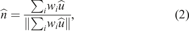
To model this behavior, neurons in the model are characterized by place sensitivity and orientation sensitivity, each of which are calculated individually and multiplied together to a generate the place cell’s total activity. In biological neurons, “sensitivity” is characterized by increased firing rate. For our model, it is represented by a scalar value. Place activity at point (x, y) is calculated by (1):

v_{place} = N (\sqrt{{(p_{x} - x)}^{2} + {(p_{y} - y)}^{2}}; 0, σ^{2}),

(1)

where the distance between the place cell location (p_x, p_y) and the agent’s location (x, y), is passed through a Gaussian activation function. The hyper-parameter σ controls how sharply the activity of the place cell decreases as the distance from the cell’s preferred location increases. This is dependent on the scale of the environment, and is set to 2.0 in our experiments. Each grid in our environment had a length of 1 unit, so this allowed for sampling in a wide range around the agent’s location.

Orientation sensitivity is defined by a response array of 8 values each representing the cardinal and ordinal directions of travel. From these values, a response vector $\hat{n}$ can be generated as:

\hat{n} = \frac{\sum_{i} w_{i} \hat{u}}{‖ \sum_{i} w_{i} \hat{u} ‖},

(2)

where

\hat{u}

is the unit vector corresponding to one of 8 directions and w_i is the value for this direction. Consistent with the experimental data in Ormond and O’Keefe (2022), values of the response array are initialized to have a preference towards the goal location. This is achieved through:

d (p, p_{0}, d) = |\frac{(p - p_{0}) \cdot d}{‖ d ‖}|

(3)

and

w_{i} = N (d (g_{x, y}, p_{x, y}, \hat{u_{i}}); 0, σ^{2}) + U (α_{\min}, α_{\max}) .

(4)

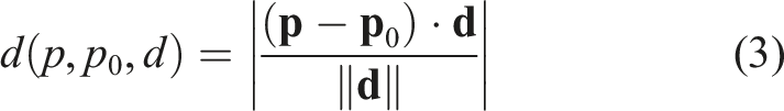
Equation (3) defines a projection function which returns the minimum distance from point p to point p₀ in the direction d and equation (4) is the initialization of response vector value w_i as the minimum distance from the place cell’s location p_x,y to the goal g_x,y through the corresponding unit vector $\hat{u_{i}}$ , plus a random amount of noise given by sampling from a random variable U with minimum and maximum values (n_min, n_max). For our experiments, (α_min, α_max) is set to (−0.5, 0.5) and σ of the activation function is set to 5.0. We found that a shallow-sloped activation function placed sufficient weight on directions that were close but not exactly in the correct direction.

In additional experiments, we examine the difference between models with goal-directed navigation and those with random initialization. In this case, ConSink cell orientation sensitivity is initialized by selecting a value uniformly between 0 and 1 for each of the 8 directions. ConSink cells then orient due to the agent’s environmental experience.

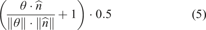
The orientation-based activation for direction θ can then be calculated as in (5), or the cosine similarity between the response vector and the orientation. This value was normalized between 0 and 1 so that we can achieve a total cell activation between 0 and 1 when it is multiplied with the place activation.

(\frac{θ \cdot \hat{n}}{‖ θ ‖ \cdot ‖ \hat{n} ‖} + 1) \cdot 0.5

(5)

Vector Navigation with ConSink Place Cells

To facilitate navigation, a population of directional place cells is initialized, each with place sensitivity for a random location in the environment as defined by equations (1) through 4. Locations of place cells are constrained such that each cell is a minimum distance from its neighbors. This minimum distance is dependent on the size of the environment and the number of place cells, and was necessary to ensure place cells are sufficiently distributed throughout the environment.

At each simulated timestep, an action is chosen by sampling the population of cells at the current location for each possible direction of travel. The values for each direction are passed through a softmax activation function to determine the probability of selecting the corresponding action. The temperature of this softmax function is set to 1.0 in our experiments.

Eligibility Trace and Reward

Learning is achieved by changing the values of the response array according to the reward signal received by the environment. To do this, each neuron must maintain an eligibility trace e defined by:

e = \{\begin{cases} v_{place} & if v_{place} > β \\ e - \frac{e}{τ} & otherwise \end{cases},

(6)

where β determines the minimum place activity to set the eligibility trace and τ determines the rate of decay of the eligibility trace. We set β to 0.5 and τ to 100 in our experiments. This β value allowed the eligibility trace of nearby neurons to be set again in the case the agent visited the same location twice in quick succession, and a large τ led to a slower decay and greater updates to neurons involved in earlier decisions.

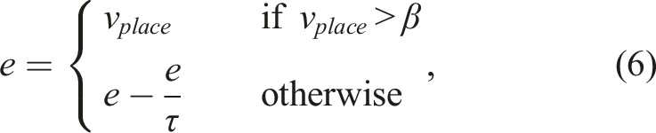
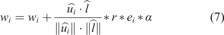
The eligibility trace of each neuron is updated after an action is taken. The purpose of this eligibility trace is to determine the contribution of each cell to the previous action, as well as solve the credit assignment problem when a reward signal is used to update the the modeled ConSink neurons. When the neuron’s eligibility trace is updated to v_place, a unit vector $\hat{l}$ between the neuron’s preferred location and the agent’s location is saved so that it can be used to update the directional sensitivity.

Upon receiving a positive or negative reward, the values of each neuron’s response arrays are calculated by:

w_{i} = w_{i} + \frac{\hat{u_{i}} \cdot \hat{l}}{‖ \hat{u_{i}} ‖ \cdot ‖ \hat{l} ‖} * r * e_{i} * α

(7)

where r is a negative or positive reward from the environment and α is a learning rate (set to 0.001 in our experiments). The cosine similarity between the saved direction of travel and the response array value’s unit vector determine its contribution to the agent’s action. The eligibility trace additionally scales the learning by how active the neuron was during traversal.

Environment

We use the OpenAI Gym framework to build environments capable of training our models and Reinforcement Learning models for comparison (Brockman et al., 2016). Agents traverse a grid-world environment and are allowed to move to neighboring squares in 8 directions if that square is not occupied by an obstacle or out of bounds. We test our algorithm in three different environments.

The first environment is the Dyna maze, which was introduced to test the Dyna Reinforcement Learning algorithm and has been used in previous navigation papers (Mattar & Daw, 2018; Sutton, 1991). Our implementation can be seen in Figure 1. The agent (green) started randomly at any space in the leftmost column of the environment, and the goal (red) was always in the top-right space.

Figure 1.

The Dyna Maze Environment. Black Squares Represent Intraversable Obstacles. Red Square is the Goal. The Agent Starts Randomly Along the Leftmost Column (the Green Square Represents One Starting Location)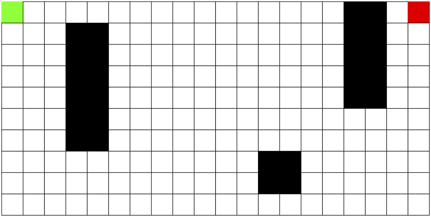

To further assess the robustness of our algorithm, we train multiple instances of the model on environments with randomly placed obstacles. Obstacles are placed randomly according to a density percentage (10% in our experiments) and then iteratively moved to ensure a valid path from the start to end exists. In this case, the agent’s start position is always on the top-left space, and the goal on the bottom-right space. A sample environment of this kind can be seen in Figure 2.

Figure 2.

A Sample Environment With Randomly Placed Obstacles at 10% Obstacle Density. The Agent’s Start Location is Always on the Top Left, and the Goal is Always on the Bottom Right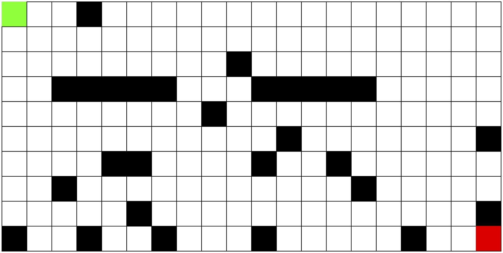

Lastly, we train models in a completely open environment similar to that used in the rat experiments (Ormond & O’Keefe, 2022), which was a 10 × 10 grid. The environment and models are initialized with the goal in the center of the environment (5, 5). The goal is moved to a different location (2, 3) after 100 epochs of training. At each episode, the agent started randomly at the edge of the environment.

Agents received an observation in the form of its current grid location (x, y) and 8 values corresponding to the distance to the closest boundary or wall in the directions of movement. The reward signal for the environments is as follows. Reaching the goal results in a reward of 1.0. Attempting to move into a space occupied by an obstacle results in a reward of −0.8, and −0.75 for attempting to move out of bounds. If the agent moves to a previously visited space, it receives a reward of −0.25. The agent receives a reward of −0.04 in all other cases. An epoch in this environment lasted until the goal is reached, or the total reward went below −100. This reward structure was chosen to encourage fast planning towards the goal while discouraging wasteful actions and encountering obstacles. Individual values were fine-tuned for convergence on our model’s comparisons. To ensure fairness, all models had the same observation space and rewards.

Comparisons

We assess the performance of our model by comparing two other SoTA RL algorithms on the same environment.

Deep Q-Networks: An RL algorithm combining the Q-learning technique and deep learning (Mnih et al., 2013). A neural network is trained to approximate the Q-function, which estimates the expected reward for taking an action at a given state. Past experiences are replayed to stabilize training and improve data efficiency. We implemented DQN with a 2 hidden layer network, with 256 neurons at each layer.

Proximal Policy Optimization: An RL algorithm with the objective of approximating an optimal policy which maps specific states to actions (Schulman et al., 2017). A neural network is trained to learn a probability distribution of each action given the agent’s current state. PPO has found great success in robotics and game playing for it’s simplicity and efficiency. We implemented PPO with a 2 hidden layer network, with 64 neurons at each layer.

Results

Maze Learning

The result of 500 epochs of training on the Dyna maze are shown in Figure 3(a). Solid lines and shaded areas represent the mean and standard error of 10 agents. Since the reward signal is overwhelmingly negative, it is expected that an agent’s total reward approaches zero as it learns to avoid obstacles and take minimal steps to reach the goal. Agents using our ConSink model learned faster than both PPO and DQN agents, as evidenced by larger reward epochs in a shorter time. This can also be seen when measuring the epoch step count, where our models consistently learned shorter paths. One reason for this is that ConSink place cells have preferred directions initially, as observed by Ormond and O’Keefe (2022).

Figure 3.

DQN, PPO, and Consink (Ours) Agents Trained on the (a) Dyna Maze Environment and (b) Random Mazes for 500 Epochs. Top Graphs are the Total Number of Steps before Reaching the Goal or Failing, Bottom Graphs are the Total Reward at Each Epoch. The Line and Shaded Area are the Mean and Standard Error of 10 Different Agents Each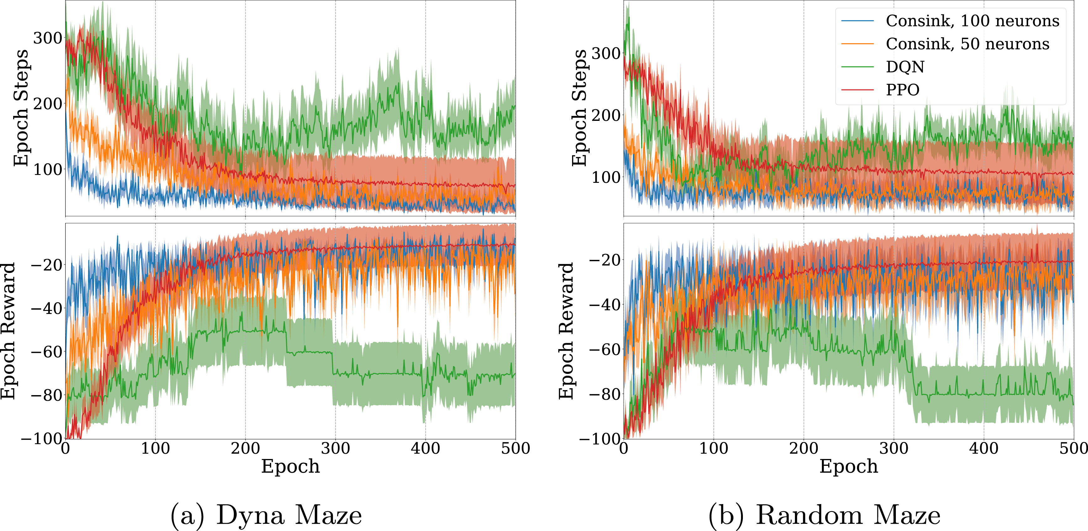

We see similar results on randomly generated mazes in Figure 3(b). Our ConSink models with both 100 or 50 neurons outpaced DQN and PPO on both total reward per epoch and steps per epoch. Despite random initialization for the environment, the location of cells, and directional sensitivity of each cell, we find striking consistency over multiple runs.

Figure 4 depicts the difference in the neurons’ directional sensitivities from initialization to the final training epoch. Place cells are drawn at their specified location, with lines indicating the direction of the response vector. Neurons in the model initially showed scattered directional sensitivity due to the noise from their initial preference towards the goal as described in section 2.1. After training, populations of nearby neurons show similar directional sensitivity to each other. Near obstacles such as the bottom-most square, the neurons’ directional sensitivities appear to curve around it, suggesting the model learns the optimal action is to avoid the obstacle while moving towards the goal.

Figure 4.

Top Image Shows the Initial Directional Sensitivity of Place Cells. Bottom Image Shows Directional Sensitivity after 500 Epochs of Training. Place Cells are Drawn in Purple, With a Line Indicating the Direction of Highest Activity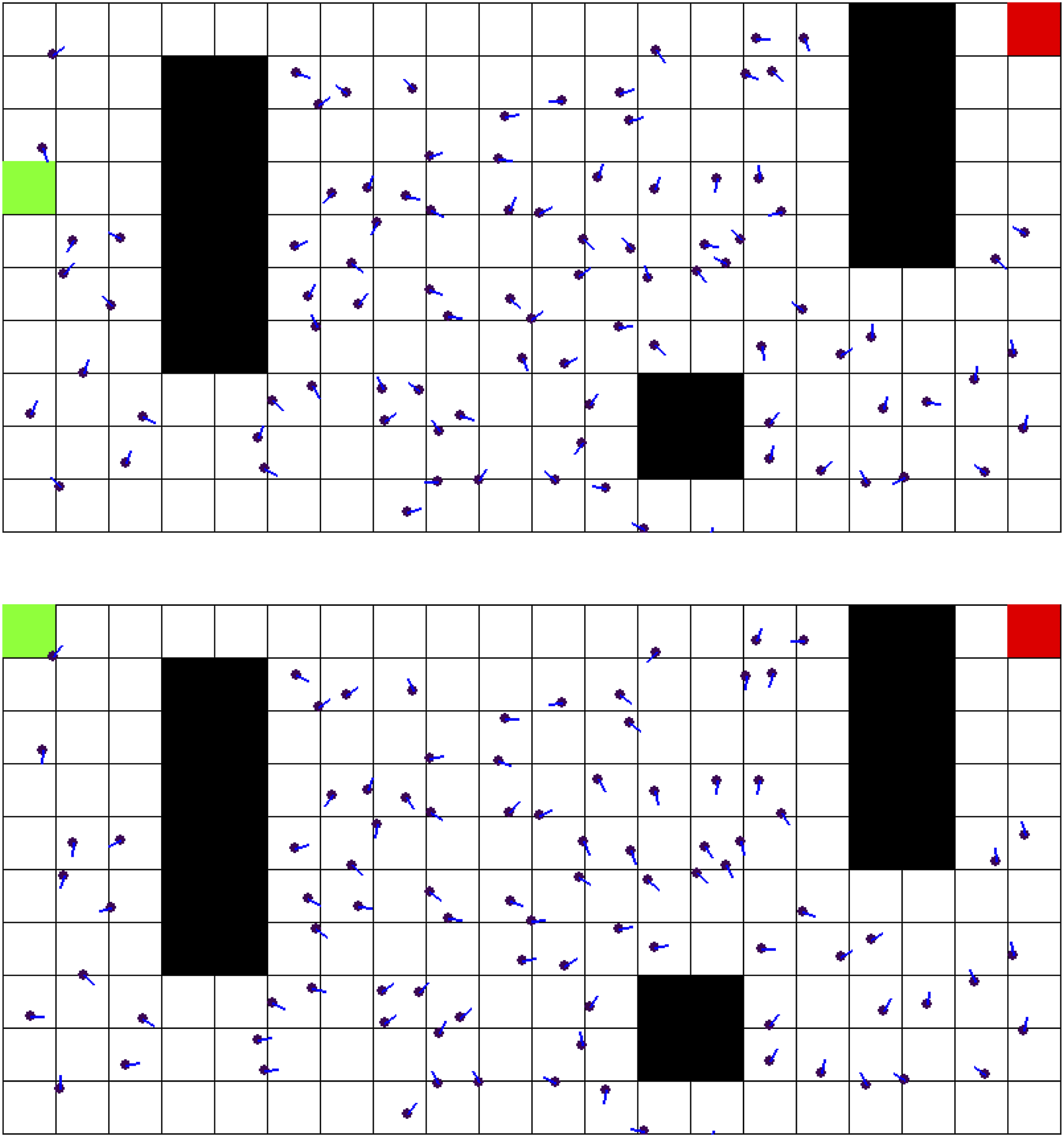

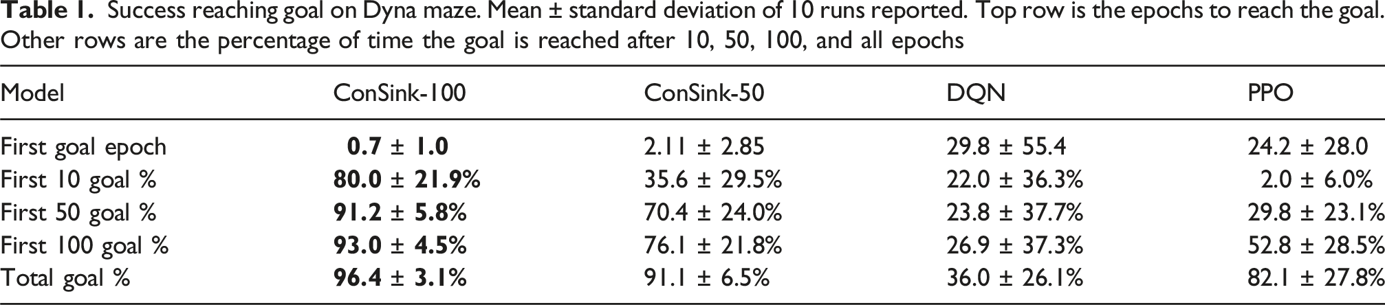
Tables 1 and 2 report the average number of epochs before each model reaches the goal for the first time, as well as the percentage of time the goal is reached after 10, 50, 100, and all epochs. Each epoch in the environment lasts until the agent reaches the goal, or the total reward goes below −100. The results are the mean of 10 different agents.

Table 1.

Success reaching goal on Dyna maze. Mean ± standard deviation of 10 runs reported. Top row is the epochs to reach the goal. Other rows are the percentage of time the goal is reached after 10, 50, 100, and all epochs

Model	ConSink-100	ConSink-50	DQN	PPO
First goal epoch	0.7 ± 1.0	2.11 ± 2.85	29.8 ± 55.4	24.2 ± 28.0
First 10 goal %	80.0 ± 21.9%	35.6 ± 29.5%	22.0 ± 36.3%	2.0 ± 6.0%
First 50 goal %	91.2 ± 5.8%	70.4 ± 24.0%	23.8 ± 37.7%	29.8 ± 23.1%
First 100 goal %	93.0 ± 4.5%	76.1 ± 21.8%	26.9 ± 37.3%	52.8 ± 28.5%
Total goal %	96.4 ± 3.1%	91.1 ± 6.5%	36.0 ± 26.1%	82.1 ± 27.8%

Table 2.

Success reaching goal on randomly generated mazes over 10 runs (mean ± stdev). Top row is the number of epochs to reach the goal. Other rows are the percentage of time the goal is reached after 10, 50, 100, and all epochs

Model	ConSink-100	ConSink-50	DQN	PPO
First goal epoch	2.3 ± 3.78	1.7 ± 2.33	10.5 ± 8.16	19.3 ± 33.47
First 10 goal %	62.0 ± 42.4%	58.0 ± 36.3%	10.0 ± 16.1%	12.0 ± 18.3%
First 50 goal %	83.2 ± 15.8%	75.6 ± 23.0%	29.4 ± 24.7%	34.2 ± 29.3%
First 100 goal %	85.6 ± 15.4%	77.5 ± 25.1%	40.0 ± 33.6%	51.5 ± 32.4%
Total goal %	86.5 ± 15.2%	79.7 ± 32.6%	36.4 ± 32.1%	74.3 ± 37.0%

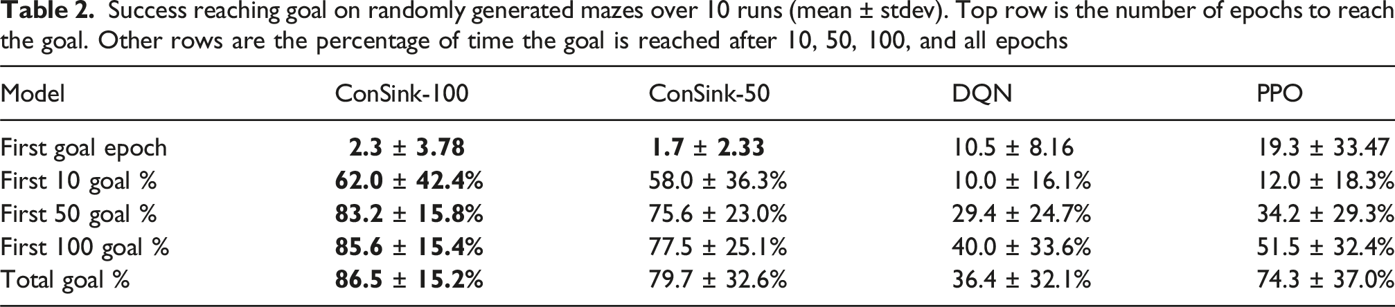
ConSink models are first to reach the goal from initialization, and reach the goal a larger percentage of the time throughout training. The speed in which our models successfully reach the goal can be attributed to a number of factors. Our models do not rely on training densely connected neural networks like DQN and PPO. Our learning rule facilitates adjustments to the model completely online, rather than during specific training times between epochs. Additionally, initializing each neuron’s directional sensitivity to be towards the goal means the model will often start by choosing actions in a straight line towards the goal, which may be correct in many cases.

Goal-Switching and Adaptability

Our experiments evaluating adaptability in an open environment are shown in Figure 5. The agents are trained for 100 epochs with the goal at (5, 5), after which the goal is moved to (2, 3). The point at which the goal is moved is indicated by the dotted red line. As with the previous experiments, the line and shaded areas represent the mean and standard error of 10 agents. Because the environment contains no obstacles and the agent can reach the goal in minimal steps, our models and DQN quickly found success navigating. After the goal switch, we see a dramatic decrease in epoch reward and an increase in epoch steps as our models initially fail to reach the new goal. However, after less than 20 epochs, they return to performing better on reward and steps taken than DQN and PPO.

Figure 5.

DQN, PPO, and Consink (Ours) Agents Trained on an Obstacle-free Open Environment for 500 Epochs. The Goal is Moved to an Alternate Location after 100 Epochs, Shown by the Dotted Line. Top Graph is the Total Number of Steps before Reaching the Goal or Failing, Bottom Graph is the Total Reward at Each Epoch. The Line and Shaded Area are the Mean and Standard Error of 10 Different Agents Each. Inset Graph Shows Training Epochs From 90 to 130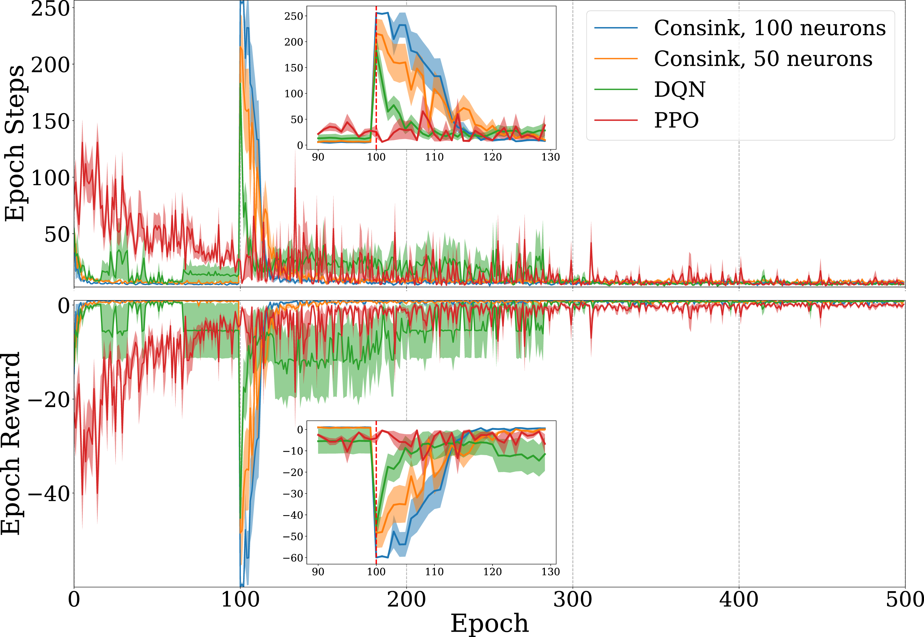

The high epoch step count and low reward from our models immediately following the goal shift can be attributed to a lack of exploratory behavior from the trained model. This could potentially be alleviated by implementing a variable softmax temperature for action selection based on the total accumulated reward in an epoch. This way, the model exploits its learned action policy unless it has accumulated negative rewards, in which case it will switch to a more explorative strategy.

Figure 6(a) shows the change in distance of the mean ConSink location to the goal before and after the goal switch. A neuron’s ConSink location is calculated by multiplying the neuron’s response vector by its distance to the goal. ConSinks are initially tuned to the location of the original goal, and over the first 100 epochs the mean ConSink location continues to shift closer to the center of the goal. After the goal switch we see the mean ConSink location shift in the direction of the new goal with training, as the place neurons’ directional sensitivities begin to change due to learning.

Figure 6.

(a) Distance of the Mean ConSink Location after the Goal is Changed in an Open Environment. Consink Agents With 100, 50, and 25 Neurons are Trained for 100 Epochs before the Goal is Changed. The Line and Shaded Area are the Mean and Standard Error of 10 Different Agents Each. (b) Visualization of Consinks before and after the Goal is Changed. Gray Circles Represent the Initial Location of Consinks and the Gray Square is the Location of the First Goal. Red Circles Represent the Consink Location of the Same Place Cell after Training on the New Goal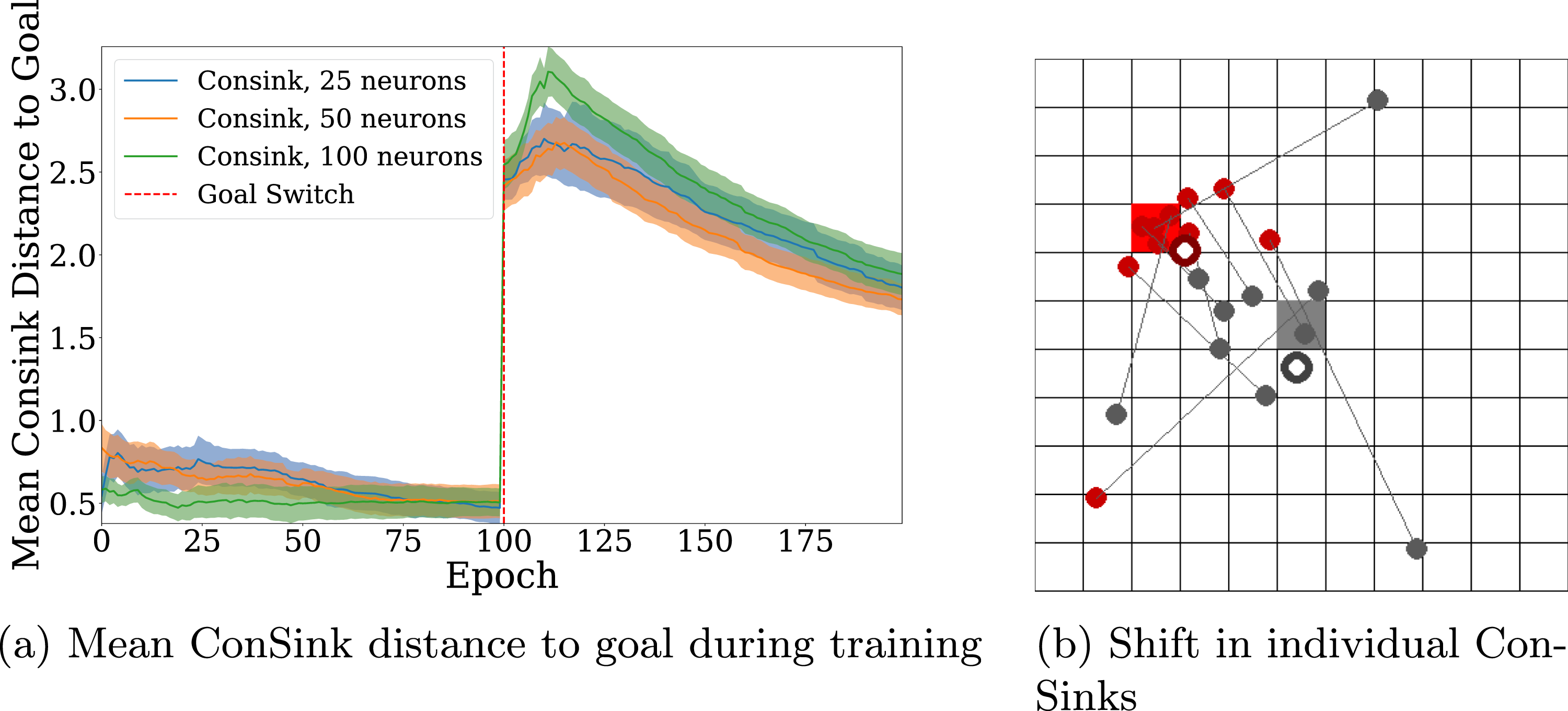

Similar to Figure 2(e) from the rodent ConSink experiments (Ormond & O’Keefe, 2022), we plot the shift of individual ConSinks before and after training in Figure 6(b). The gray square is the location of the initial goal. Filled gray circles are the locations of ConSinks for 10 candidate neurons, and the white-filled gray circle is the mean ConSink location for the entire population. The same is true for the red square and red circles, which represent the new goal and ConSinks after the goal is changed. Gray lines connect the ConSinks of the same neuron. We find that individual ConSinks move closer to the new goal during training, leading the mean ConSink location to shift as well.

ConSink Initialization

We investigated the effects of ConSink initial directional sensitivity on performance in the same environments. DQN and PPO did not have prior knowledge of the environment, however the ConSink neurons in the previous sections were initialized to point near the goal as detailed in 2.1. While this mimics what was observed in biological recordings, it is possible that these initial conditions gave the ConSink models an unfair advantage for locating the goal in early trials. To test this, we initialized the ConSink response arrays to have random directional sensitivity.

The ConSink model with random initialization learned faster and had better performance than DQN and PPO. Similar to previous experiments, we trained the models for 500 epochs on both the Dyna maze (Figure 7(a)) and randomly generated mazes (Figure 7(b)). In the case of the Random Maze, all models were trained again so they could be evaluated on the same maze configurations. Despite not having prior information about the location of the goal in the randomly initialized case, our models were still capable of finding and navigating using the reward signals in less time than the reinforcement learning models. Because the directional sensitivity adjusts in response to negative reward, the ConSink models rapidly learn to move away from obstacles and walls, allowing it to find the goal in relatively few epochs.

Figure 7.

ConSink Models With Random Initialization Against DQN and PPO (a) Dyna Maze Environment and (b) Random Mazes for 500 Epochs. Top Graphs are the Total Number of Steps before Reaching the Goal or Failing, Bottom Graphs are the Total Reward at Each Epoch. The Line and Shaded Area are the Mean and Standard Error of 10 Different Agents Each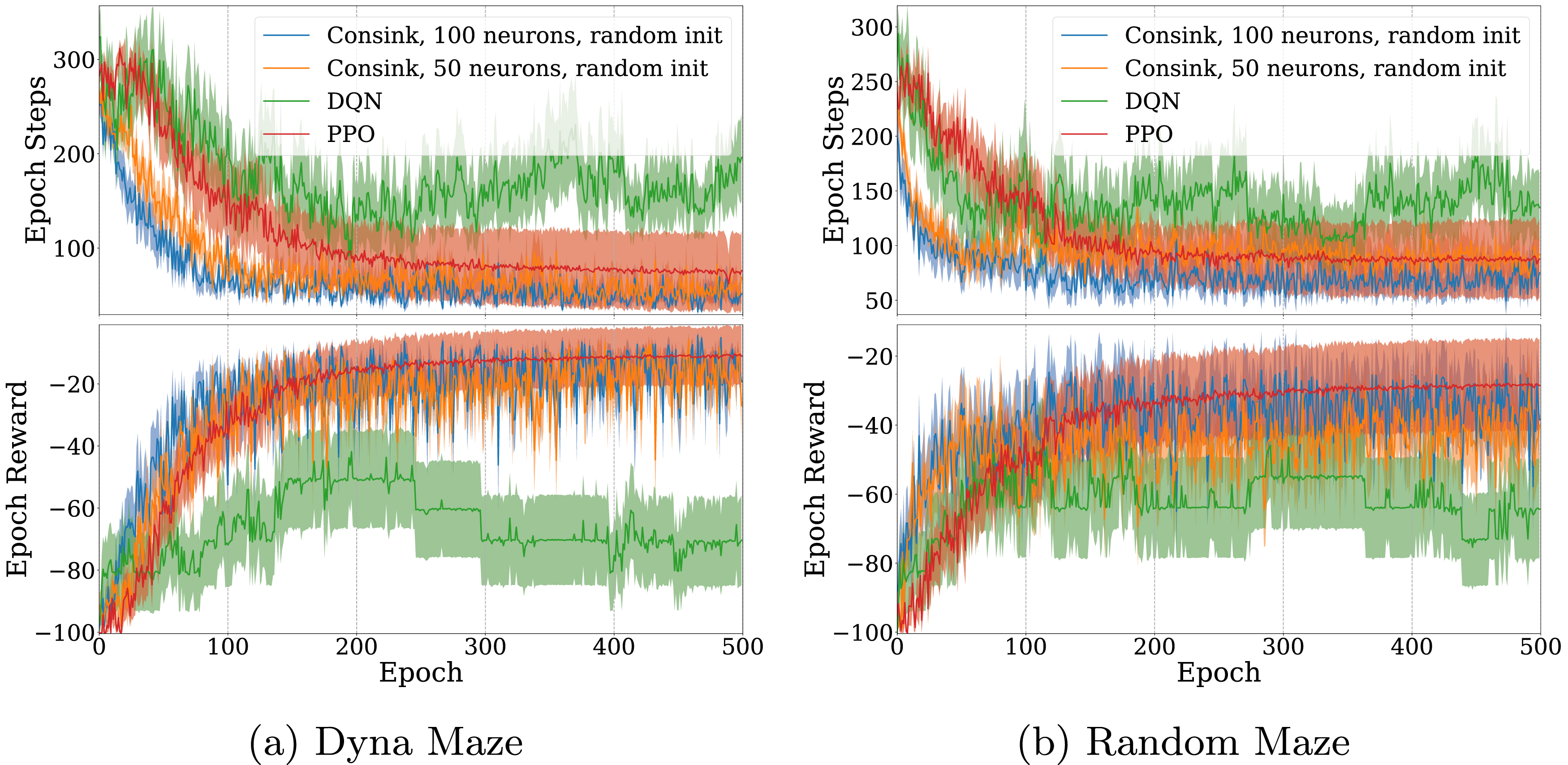

We also compared model size between the random initialization and the goal-directed initialization versions of the model. For the Dyna maze (Figure 8(a)), we found that in both the random and goal-directed initialization case, models with 100 neurons learned faster than their 50 neuron counterparts. Random initialization resulted in slightly slower learning, but did not affect the performance after sufficient training (8b). This property also held for agents trained on the randomly generated mazes. Agents with goal-directed initialization learned faster than those with the same number of neurons and random initialization. However, agents with more neurons reached a larger maximum reward and minimum number of steps to reach the goal.

Figure 8.

ConSink Models With 50 or 100 Neurons and Random or Goal-Directed Initialization Trained on (a) Dyna Maze Environment and (b) Random Mazes for 500 Epochs. Top Graphs are the Total Number of Steps before Reaching the Goal or Failing, Bottom Graphs are the Total Reward at Each Epoch. The Line and Shaded Area are the Mean and Standard Error of 10 Different Agents Each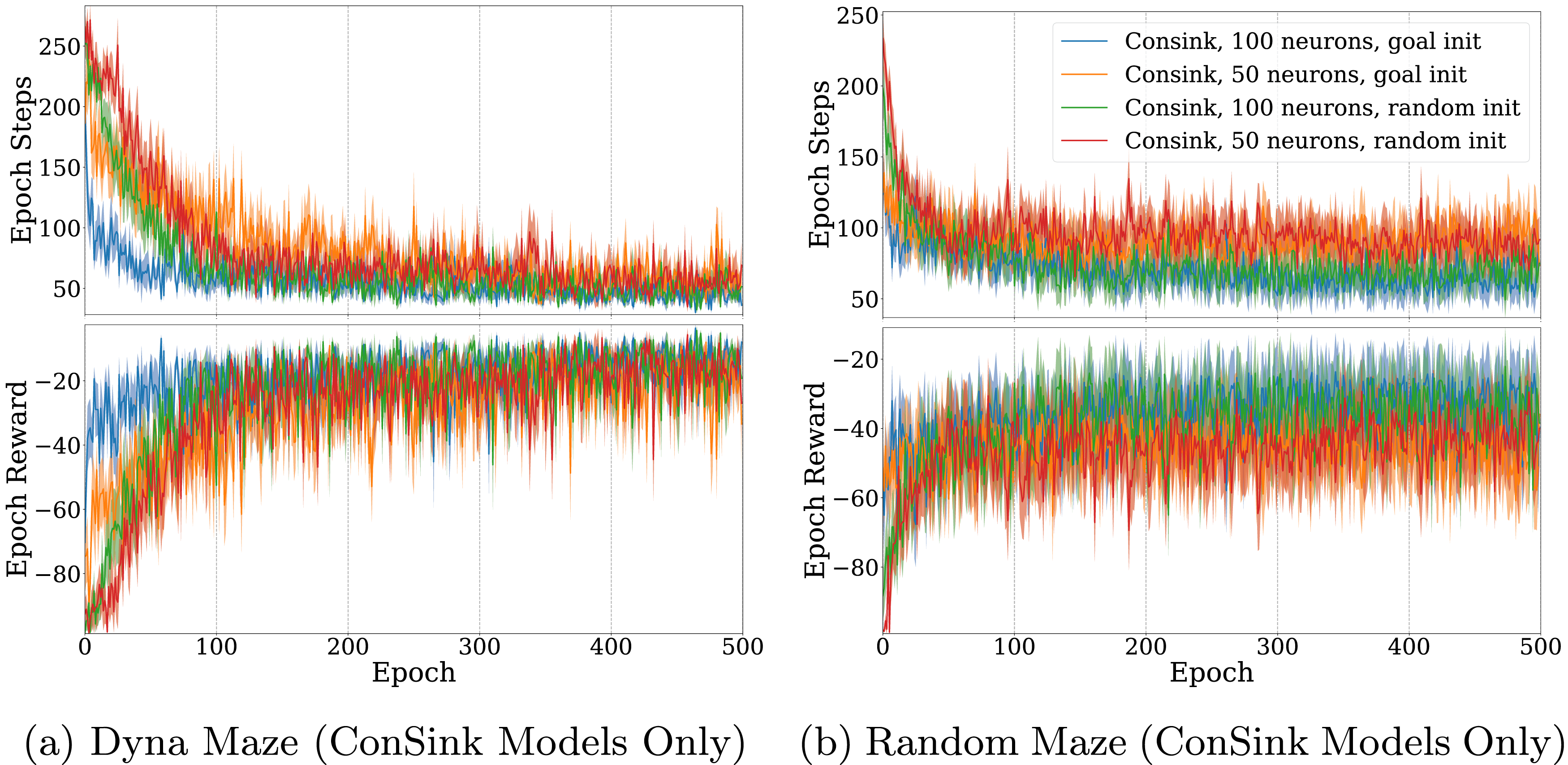

Our experiments in Figure 9 further confirmed these properties across model sizes between 50 and 100 neurons. In both the Dyna maze and randomly generated maze cases, the average epoch step count decreased and average epoch reward increased as the number of neurons in the model increased. We also see that random initialization had a greater effect on the early stages of training (Epochs 0-100), but didn’t have an effect on the model performance in the late stages (Epochs 100-500).

Figure 9.

ConSink Models With Varying Amounts of Neurons Trained on (a) Dyna Maze Environment and (b) Random Mazes for 500 Epochs. Top Graphs are the Total Number of Steps before Reaching the Goal or Failing, Bottom Graphs are the Total Reward at Each Epoch. Orange and Blue Lines Represent Models With Goal-Directed and Random Initialization for the First 100 Epochs. Dotted Green and Dotted Red Lines Represent the Models for Epochs 100 to 500. The Line and Shaded Area are the Mean and Standard Error of 10 Different Agents Each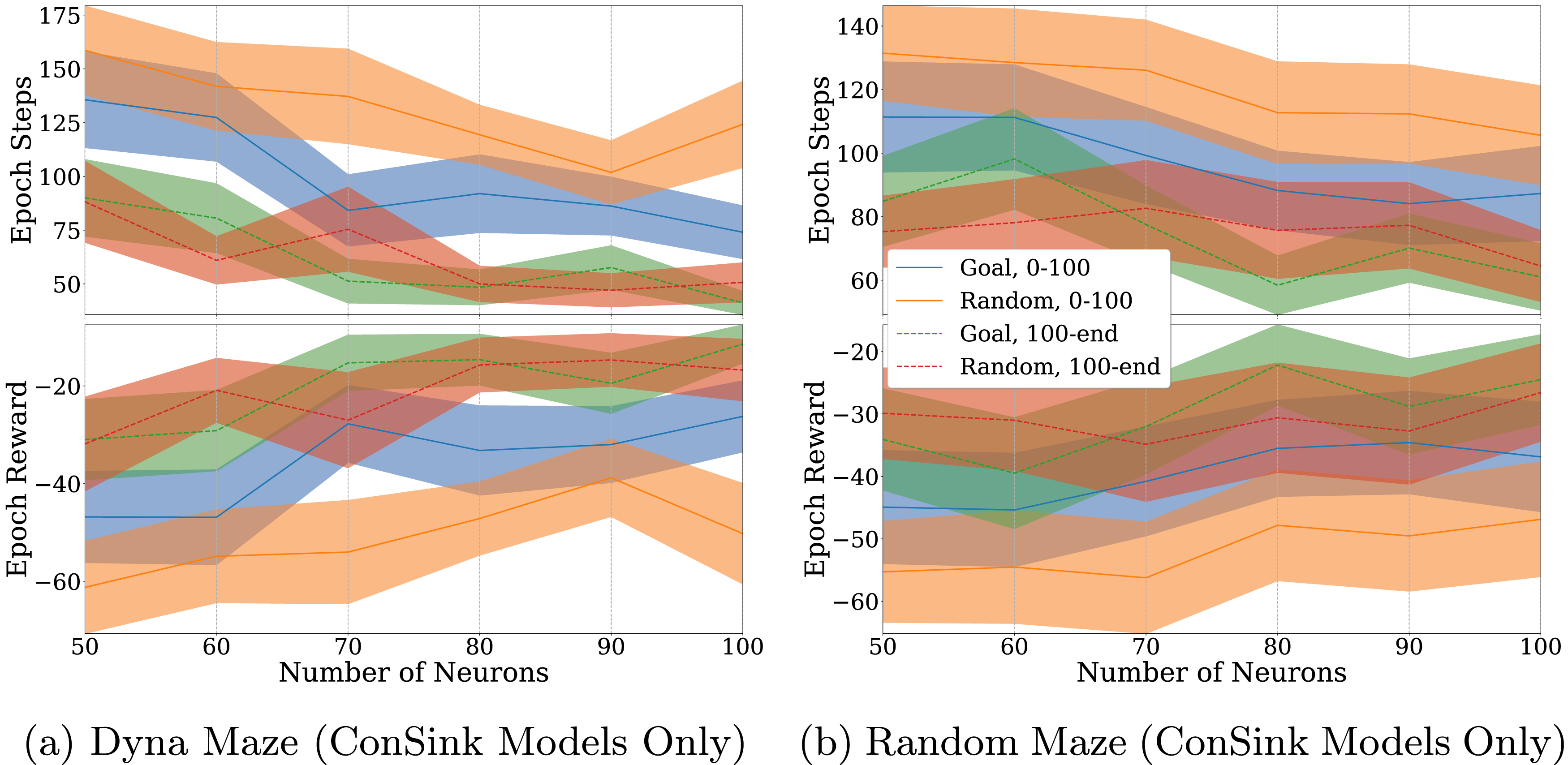

In the case of the Dyna maze (Figure 9(a)), the performance decrease due to random initialization on early stages of training was worse for 100 neuron models compared to 50 neuron models. However, in the randomly generated mazes (Figure 9(b)), the effect of random initialization remained constant. We hypothesize that the Dyna maze was more hindered by random initialization because of the large amount of open space between obstacles. This effect became more apparent in larger models, as it placed be a large amount of neurons in open space that would take longer to learn, as obstacles that incur a negative reward are farther away.

Discussion

Inspired by recent findings of ConSink place cells in the rodent hippocampus, we introduce a navigation algorithm capable of rapidly and accurately reaching a goal in obstacle-filled environments. Our model outperforms SoTA reinforcement learning models in maximizing accumulated reward, minimizing steps taken, consistently reaching the goal throughout training. When the goal is moved after training in a completely open environment, our model is able to adapt to this change in fewer epochs of exploration. Cells in our model also exhibit behavior reminiscent of biological data, as the mean ConSink location moves towards the new goal during training.

Our findings are comparable to neurophysiological recordings showing adaptation in the ConSink cells during rat maze navigation. Our novel learning rule achieves this using a combination of eligibility trace, saved trajectories, and reward signal. This suggests that ConSink place cells in the hippocampus may be employing similar reward-based learning to adjust their directional sensitivity.

Our results make interesting predictions about the role of directionally sensitive place cells in complex environments. Previous work investigating place cell directionality in rats were in environments in which a direct route to the goal was always possible (Jercog et al., 2019). Ormond and O’Keefe used a unique “honeycomb maze” in which the rat was required to make a sequence of binary choices on raised platforms, sometimes requiring the rat to move away from a goal (Ormond & O’Keefe, 2022). In our simulations, we introduced obstacles and circuitous routes to goals.

In the rodent experiments, the environment did not have obstacles and was fully visible to the rat. The honeycomb maze removed the ability for the rat to move directly to the goal, however the correct binary choice was always more in the direction of the goal than the incorrect one. Our model predicts that, in environments filled with obstacles, populations of ConSinks near obstacles blocking direct routes to the goal may need to point towards sub-goals in order to facilitate navigation. Behavioral studies have shown that mice utilize sub-goal strategies when learning new environments (Shamash et al., 2021). Future work might investigate if sub-goal memorization is encoded in place cell directionality.

Our model also raises the question of whether or not directional polarization is tuned away from “negative rewards” such as noxious locations or obstacles in the same way it is tuned towards goal locations. This was necessary for our model to solve the mazes, as it caused ConSink locations to shift away from obstacles in order to navigate around them. This property has yet to be demonstrated in biological cells. It was shown that place cells in the lateral septum (LS) were skewed asymmetrically depending on the direction of travel towards or away from a reward site (Wirtshafter & Wilson, 2020). LS place cells fired ahead of the animal when traveling towards a goal, but fired behind the animal when traveling away from the goal. Although this doesn’t directly encode negative stimuli, it demonstrates a potential encoding of the difference between actions which lead the animal away from positive reward versus towards it.

We also shed light on the role of place cell density and directional sensitivity in the context of goal-directed navigation. The recruitment of place cells has been shown to be proportional to the size of the environment up to 8.75 m² (Tanni et al., 2022). The same study finds that around boundaries, place cells were recruited in greater number but had smaller place fields, while in the center of the environment place cells had larger fields but were less numerous. Interestingly, this tradeoff of place field size versus number of cells was balanced such that the proportion of co-active place cells was consistent throughout locations in the environment. While this particular study did not look at place cells with directional sensitivity, Ormond and O’Keefe (2022) found that anywhere between 27–35% of the neurons they recorded had directional polarization. Future neuroscience experiments may investigate whether this proportion is maintained across different environmental sizes, and whether the presence of obstacles affects the density and sensitivity of directional polarization in the same way as what was observed with regular place cells.

This property of greater place cell density and smaller place fields around boundaries would be beneficial to our model as well. Given that the model navigates by sampling from nearby place cell directional sensitivities, densely packed place cells around boundaries would facilitate more careful navigation around obstacles than in open space. While there were no obstacles present in studies which identified directional place cells, our results suggest that directional selectivity away from obstacles is key for navigating in complex environments. For this reason, we predict that place cells near obstacles, particularly those around the goal, will be more densely packed than in the open portions of the environment.

Our model is similar to traditional Q-learning in that each place neuron is learning an optimal action for the location it is sensitive to, much like a Q-table learns optimal actions for each state. However, our model uniquely takes advantage of the fact that environment states in a navigational problem can be related over two axes of position. This allows for the generalization of unlearned areas by sampling the learned actions of place cells representing nearby areas. Future work may aim to apply our model to non-navigational problems which can be represented in this way. The model may also employ heterogeneous learning rates and eligibility trace functions across neurons to represent dynamic environments.

Deep Q-learning uses a form of experience replay in which previously saved state-action-reward sequences are used to train the model multiple times. PPO employs a similar technique, maintaining a growing replay buffer which is used to train the model every set number of epochs. While such a replay system is not yet implemented in our model, recordings of the rat hippocampus have shown sequential reactivation of place cells resembling past trajectories during sleep or rest states (Lee & Wilson, 2002). By saving past experiences, replay can potentially be used to further improve the efficiency of our models. Additionally, the model can serve as a generator for novel trajectories by continually sampling and simulating actions offline.

In conclusion, ConSink cells have the potential for practical applications ranging from machine learning to robotics. Future simulations of ConSink cells in spatial and non-spatial environments could inform neuroscience on the function of these novel neurons.

Footnotes

ORCID iDs

Harrison Espino

Jeffrey L. Krichmar

Funding

The authors disclosed receipt of the following financial support for the research, authorship, and/or publication of this article: This work was supported by the National Institute of Neurological Disorders and Stroke (NINDS) Award No. R01NS135850.

Declaration of Conflicting Interests

The authors declared no potential conflicts of interest with respect to the research, authorship, and/or publication of this article.

Author Biographies

Harrison Espino received a B.S. in Computer Science and Cognitive Science from the University of California, Davis in 2021, and is currently pursuing a Ph.D. in Computer Science at the University of California, Irvine. His research lies at the intersection of robotics, neuroscience, and machine learning, with a particular focus on biologically inspired algorithms for autonomous navigation. Espino is the lead or co-author of peer-reviewed publications in IEEE and Springer Nature venues, including work on spiking neural networks for path planning, biologically inspired algorithms, and replay mechanisms for improving exploration. He has presented his work at both top robotics conferences such as the IEEE International Conference on Robotics and Automation (ICRA) and interdisciplinary workshops like the National Institute of Health (NIH) BRAIN NeuroAI Workshop.

Jeffrey L. Krichmar received a B.S. in Computer Science in 1983 from the University of Massachusetts at Amherst, a M.S. in Computer Science from The George Washington University in 1991, and a Ph.D. in Computational Sciences and Informatics from George Mason University in 1997. Krichmar has over 20 years of experience designing adaptive algorithms, creating neurobiologically plausible neural networks, and constructing brain-based robots whose behavior is guided by neurobiologically inspired models. He has over 160 publications and holds 9 patents. His work has been funded by the Defense Advanced Research Projects Agency (DARPA), Intelligence Advanced Research Projects Activity (IARPA), National Science Foundation, and the Air Force Office of Scientific Research. Additionally, he has worked with industry on sponsored research contracts from Qualcomm, Northrup Grumman Corporation, and Toyota Motor North America. He is a Senior Member of IEEE and the Society for Neuroscience. He recently published a book, “Neurorobotics: Connecting the Brain, Body, and Environment” that lays out principles for designing intelligent systems.

References

Brockman

Cheung

Pettersson

Schneider

Schulman

Tang

Zaremba

(2016). Openai gym. CoRR, abs/1606.01540.

Lillicrap

Sutskever

Levine

(2016). Continuous deep q-learning with model-based acceleration. In Balcan

M. F.

Weinberger

K. Q.

(Eds.), Proceedings of the 33rd international conference on machine learning, volume 48 of proceedings of machine learning research (pp. 2829–2838). PMLR.

Harrison

Krichmar

J. L.

Vector-based navigation inspired by directional place cells. In Brock

Krichmar

(Eds.), From animals to animats 17. SAB 2024. Lecture notes in computer science (pp. 27–38). Springer. https://doi.org/10.1007/978-3-031-71533-4_3

Jercog

P. E.

Ahmadian

Woodruff

Deb-Sen

Abbott

L. F.

Kandel

E. R.

(2019). Heading direction with respect to a reference point modulates place-cell activity. Nature Communications, 10(1), 2333. https://doi.org/10.1038/s41467-019-10139-7

Lee

A. K.

Wilson

M. A.

(2002). Memory of sequential experience in the hippocampus during slow wave sleep. Neuron, 36(6), 1183–1194. https://doi.org/10.1016/s0896-6273(02)01096-6

Lin

C.-J.

Jhang

J.-Y

Lin

H.-Y.

Lee

C.-L.

Young

K.-Y.

(2019). Using a reinforcement q-learning-based deep neural network for playing video games. Electronics, 8(10), 1128. https://doi.org/10.3390/electronics8101128

Mattar

M. G.

Daw

N. D.

(2018). Prioritized memory access explains planning and hippocampal replay. Nature Neuroscience, 21(11), 1609–1617. https://doi.org/10.1038/s41593-018-0232-z

Mnih

Kavukcuoglu

Silver

Graves

Antonoglou

Wierstra

Riedmiller

M. A.

(2013). Playing atari with deep reinforcement learning. CoRR, 5602. abs/1312.

Ormond

O’Keefe

(2022). Hippocampal place cells have goal-oriented vector fields during navigation. Nature, 607(7920), 741–746. https://doi.org/10.1038/s41586-022-04913-9

10.

Sarel

Finkelstein

Las

Ulanovsky

(2017). Vectorial representation of spatial goals in the hippocampus of Bats. Science, 355(6321), 176–180. https://doi.org/10.1126/science.aak9589

11.

Schulman

Wolski

Dhariwal

Radford

Klimov

(2017). Proximal policy optimization algorithms. CoRR, abs/1707.06347.

12.

Shamash

Olesen

S. F.

Iordanidou

Campagner

Banerjee

Branco

(2021). Mice learn multi-step routes by memorizing subgoal locations. Nature Neuroscience, 24(9), 1270–1279. https://doi.org/10.1038/s41593-021-00884-8

13.

Sutton

R. S.

(1991). Dyna, an integrated architecture for learning, planning, and reacting. ACM SIGART Bulletin, 2(4), 160–163. https://doi.org/10.1145/122344.122377

14.

Tanni

de Cothi

Barry

(2022). State transitions in the statistically stable place cell population correspond to rate of perceptual change. Current Biology, 32(16), 3505–3514. https://doi.org/10.1016/j.cub.2022.06.046

15.

Wirtshafter

H. S.

Wilson

M. A.

(2020). Differences in reward biased spatial representations in the lateral septum and hippocampus. eLife, 9(4), e55252. https://doi.org/10.7554/elife.55252

Adaptive,Goal-Oriented Navigation Using a Model of Directionally-Polarized Place Cells

Abstract

Keywords

Introduction

Methods

ConSink Place Cell Model

Vector Navigation with ConSink Place Cells

Eligibility Trace and Reward

Environment

Comparisons

Results

Maze Learning

Goal-Switching and Adaptability

ConSink Initialization

Discussion

Footnotes

ORCID iDs

Funding

Declaration of Conflicting Interests

Author Biographies

References