Sage Journals: Discover world-class research

Abstract

Prediction is an important foundation of cognitive and intelligent behavior. However, how such predictive capabilities emerged from simple organisms has not been investigated fully. Our prior works have shown the relationship between input delay and predictive function. Furthermore, we showed that environmental change can help predictive properties to evolve. In this paper, we investigate two other key factors contributing to the evolution of prediction. We set up a reaching task with a two-segment articulated arm with the goal of touching a moving target. In Task 1, the target’s location is received with a delay in the sensors. In Task 2, we introduced occlusion in the form of input blank-out. When the hand is too close to the moving target, the target disappears from the sensors, and reappears when it is farther than a threshold. In both tasks, prediction is needed to keep track of the target’s correct location. For the controller, we used the NeuroEvolution of Augmenting Topologies (NEAT) algorithm. Our results from Task one indicate that an important fitness criterion for the emergence of predictive behavior is energy conservation. The results from Task two show that more occlusion leads to network types with stronger predictive power become more successful. Through our prior and current experiments, we identified four seemingly unrelated and unlikely factors that may have led to the evolution of prediction: delay, environmental change, energy constraint, and occlusion. These are prevalent conditions in the natural environment, thus it seems inevitable that predictive capabilities will emerge in evolving agents.

Keywords

prediction evolution neuroevolution fitness

Introduction

Prediction forms an important foundation of cognitive and intelligent behavior Bubic et al. (2010); Tjøstheim and Stephens (2022); Tani (2016). Recent advances in deep learning heavily depend on prediction, in the form of self-supervised learning based on prediction and reinforcement learning (e.g., reward prediction) Shwartz Ziv and LeCun (2024); Stachenfeld et al. (2017).

However, how such predictive capabilities emerged from simple organisms through evolution has not been investigated sufficiently Korb et al. (2016); Oudeyer and Smith (2016). Furthermore, what kind of external/internal factors and constraints could have influenced the development of prediction is unclear. Our prior works have suggested the relationship between input delay and predictive function for its compensation Lim and Choe (2006); Mann and Choe (2010). We have also shown that predictive dynamics emerge in evolved neural network controllers when environmental conditions change Kwon and Choe (2008); Yoo et al. (2014).

In this paper, we investigate two other key factors that may contribute to the emergence of predictive behavior in evolving neural networks: (1) energy and (2) occlusion (Figure 1). We set up a reaching task with a two-segment articulated arm, and conducted two different tasks.

Figure 1.

Factors Contributing to the Emergence of Prediction. The Four Factors, Proposed in This Paper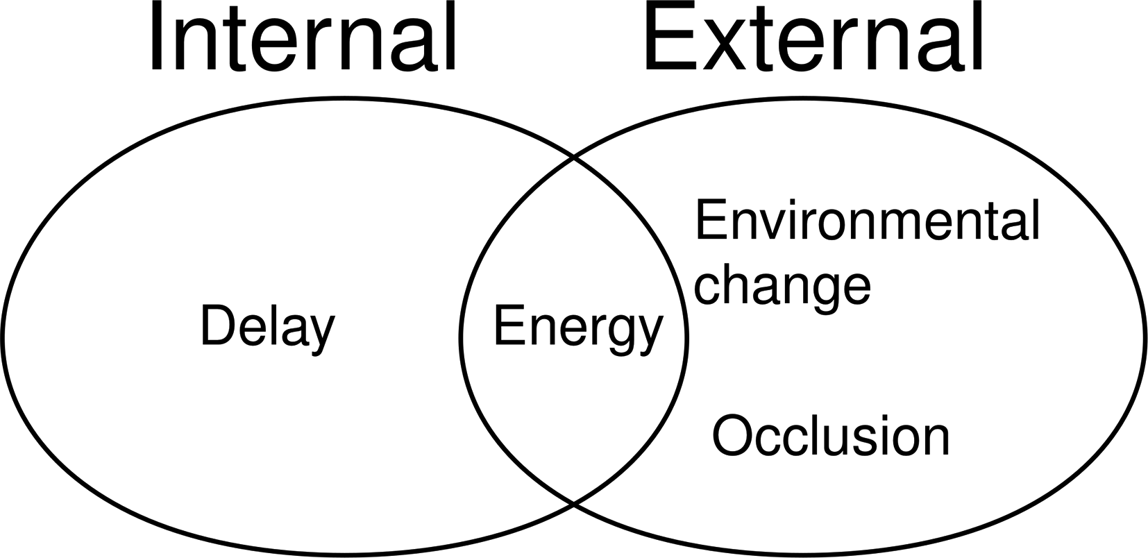

(1) In Task 1, we added input delay Li et al. (2015). (Note that predicting an unknown true location like this is different from predicting the sensory consequence of action, which requires the true sensory input to compute the prediction error, as in Tani (2016).) The arm is controlled to reach a moving target, where the target’s coordinate information is received with a fixed delay. Following our previous work Li et al. (2015), we introduced a tool to extend the reach, when the target is beyond the arm’s reach. This task is not solvable without predicting the trajectory of the moving object, since reaching for the coordinate location based on the immediate input would lead to a location previously occupied by the moving object. For the controller, we used the NeuroEvolution of Augmenting Topologies (NEAT) algorithm Stanley and Miikkulainen (2002) (cf. CTRNN Tani (2016) and FORCE Sussillo and Abbott (2009); Kashyap et al. (2018)).

(2) In Task 2, we introduced input blank-out Mehta and Schaal (2002), where the input is made invisible for a short period of time during a control task. This is similar to disappearance due to occlusion in the real world, when an agent is tracking the movement of another target agent and needs to predict when and where it will reappear, thus requiring prediction. The task is the same reaching task as above, but the target is now visible under some condition and invisible under other conditions. The controller will again be evolved using NEAT.

For Task 1 (the delayed reaching task), our results indicate that an important (auxiliary) fitness criterion for the emergence of predictive behavior is that of reduced energy usage (in the form of economy of motion). Further analysis shows that the number of recurrent loops correlate with target reaching performance, but more strongly so with the energy constraint.

For Task 2 (the input-blanking during reaching task), we find that longer input blanking (or longer occlusion) leads to network architectures that can predict to be more successful (i.e., recurrent neural network are more successful than feed-forward networks).

We expect our findings to lead to further investigations on the role of energy constraints and occlusion on the evolution of predictive behavior. Putting together our previous research and the new results reported in this paper, we can summarize the various factors that may have contributed to the emergence of prediction as shown in Figure 1.

This paper is a significantly expanded version of our previously published conference paper Kang et al. (2024). The introduction and background has been expanded to provide a full context, and one additional task (Task 2) and experimental results have been newly added. The discussion section has also been expanded.

Background

In this section, we will briefly review existing works relating to the evolution of prediction, and provide an overview of the NEAT algorithm, which we will use.

Prior Work: Delay and Environmental Change

As mentioned in the introduction, we have done some prior work in this area, showing that delay and environmental change can contribute to the emergence of prediction. Here, we will provide a bit more detail on these earlier findings.

Delay

Delay is generally considered harmful and it is something to be avoided in engineering systems, but it is prevalent in nature, including all nervous systems. Interestingly enough, it appears that delay in the system may facilitate the emergence or predictive properties, thus serving a useful purpose.

In our earlier work Mann and Choe (2010), we evolved a simple ANN controller in the classical 1D pole balancing task (Figure 2(A)). To test the effect of delay in the input line, we varied the delay from 0 ms (no delay) to 1000 ms at 200 ms interval (the x-axis in Figure 2(B)). In each condition, the hidden unit activations at a specific time step in the trial and the sensory states in the following time step were recorded. Each sensory variable was associated with the hidden unit with the highest correlation, and the average of these values was used as the measure of how well the controller’s hidden state predict the future (the y-axis in Figure 2(B)). As we can see, longer delay leads to stronger predictive power in the evolved neural network controllers. This makes sense, because aside from the immediate task of controlling the cart, with delay, it now becomes necessary to predict the present state of the system from the information from the past.

Figure 2.

Delay Leads to Predictive Property. (A) The 1D Pole Balancing Task. (B) Amount of Delay Added to the Controller’s Input (x-Axis) versus the Correlation Between the Controller Neural Network’s Hidden State With Future State of the System (y-Axis). Adapted From Mann and Choe (2010)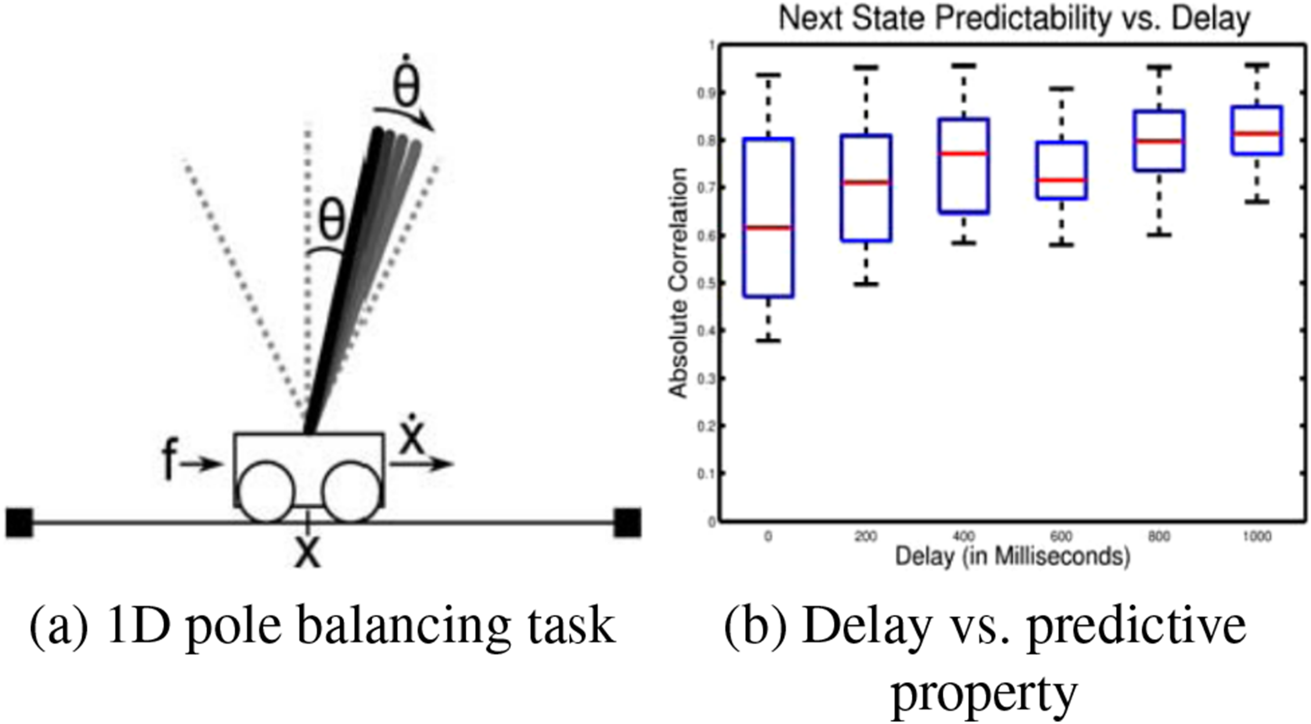

Environmental Change

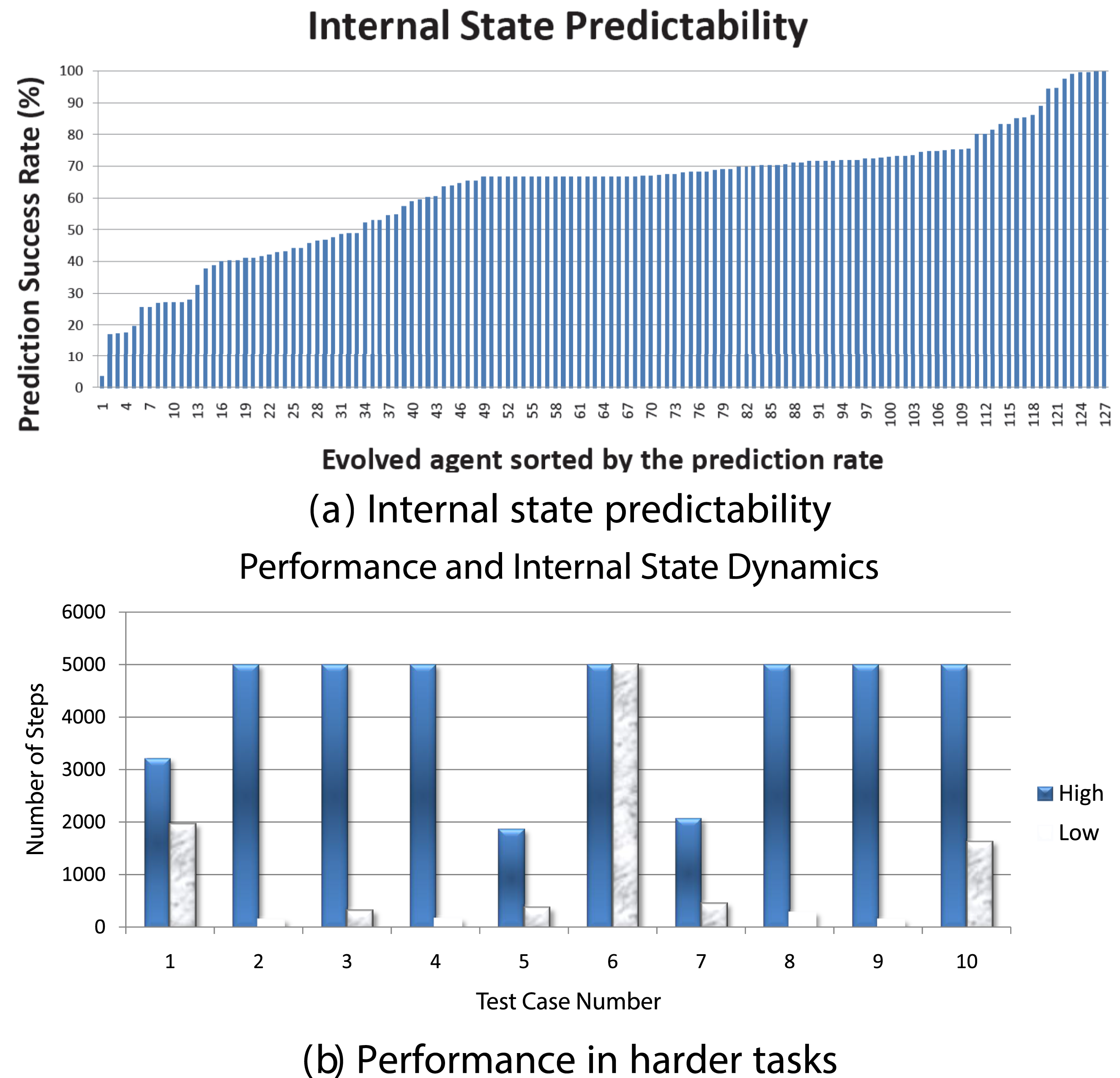
In our prior work, we studied the emergence of predictive properties in neural network controllers Kwon and Choe (2008); Choe et al. (2012); Kwon and Choe (2009). Figure 3 shows a general overview of the task and analysis framework. First, we evolved recurrent neural networks to control a cart in a 2D pole balancing task (Figure 3(A)). Once high-performance individuals emerged, we analyzed their internal state dynamics (Figure 3(B), (C), (D)). Predictability of the internal state trajectory (activity of three hidden neurons over time) was measured by training a supervised learning algorithm (backpropagation) and observing the training error, where the inputs to the predictor network were past activity values and the target output was the current activity value (Figure 3(C)). We found that there is a varying degree of predictability to these internal state trajectories (Figure 4(A)). All these individuals, regardless of the predictability of their internal states, have the same performance (meet a fixed performance criterion) since that is how they were selected (Figure 3(D)). However, once the task environment changes slightly, those with high predictability were able to maintain their performance while those with low predictability showed degraded performance (Figure 4(B)). We further tested these ideas by analyzing human EEG data Yoo et al. (2014). Interestingly, we found that predictive dynamics properties in the EEG signal are correlated with conscious states (awake or dreaming). These results suggest that dynamic properties of the internal state can hold important clues to the adaptive success of evolved neural controllers.

Figure 3.

Predictability of Internal State Trajectory in a Pole-Balancing Controller Network. ISP: Internal State Predictability. Adapted From Choe et al. (2012)

Figure 4.

Internal State Predictability and Task Performance (a) the Internal State Predictability Varies Among 130 High-Performance Individuals. (b) Under Harder Task Conditions (Larger Initial Tilt of the Pole), Performance is Higher for Individuals With High Internal State Predictability (Blue) Compared to Those With Low Internal State Predictability (gray). Adapted From Kwon and Choe (2008)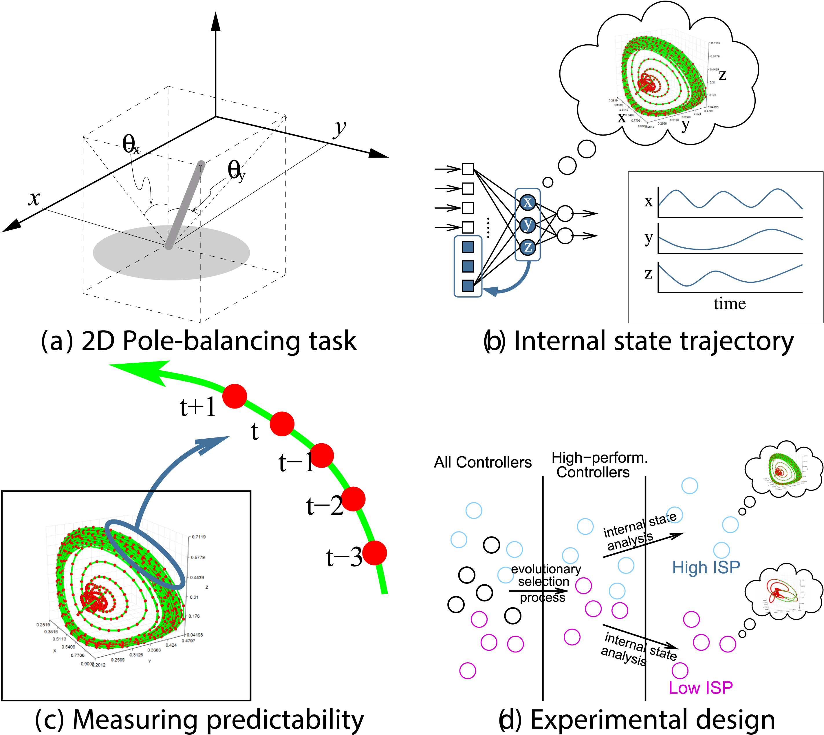

Related Works on Evolution of Prediction

Aside from the above, few papers that discuss prediction in an evolutionary context include Korb et al. (2016) and Oudeyer and Smith (2016). Korb et al. (2016) mentioned the lack of computational studies on evolution of prediction, and proceed to propose how utility and predictive capabilities can co-evolve in a simulated agent. The work is based on the “Gap Theory” in evolutionary economics which exactly states the co-evolutionary nature of utility and prediction. Oudeyer and Smith (2016), on the other hand, observed that curiosity (a form of intrinsic motivation) helps in the improvement of prediction, and these developmental structures can constrain evolution in return. Thus, the work is more about the emergent predictive ability shaping evolution, not about how evolution gives rise to predictive abilities.

NeuroEvolution of Augmenting Topologies (NEAT)

Topological neuroevolution methods evolve both topology and weights of neural networks. Our perspective is that natural evolution includes changes in the network topology in the brain, thus they mimic the natural evolution better than traditional weight-only neuroevolution methods. Moreover because the functionality of a neural network can be constrained by its topology, allowing the topology to evolve will set free the structural constraints and result in new capabilities such as recurrent dynamics. Amongst many variations of such an approach Whitley et al. (1993); Gruau et al. (1996); Yao (1999), we will use NeuroEvolution of Augmenting Topologies (NEAT) because of its advantages over other topological evolution methods Stanley and Miikkulainen (2002). Figure 5 illustrates the main concepts of NEAT.

Figure 5.

NEAT. (A) Nodes and Connections are Separately Encoded. (B) Connections With the Same Innovation Number can Be Crossed Over. Adapted From Stanley and Miikkulainen (2002)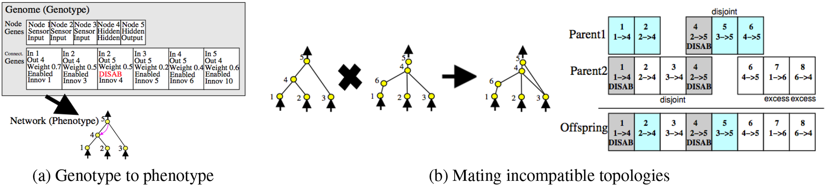

Historical marking is a major feature in the NEAT algorithm. By enumerating each innovation, NEAT solves the competing conventions problem, which is one of the main problems in neuroevolution Whitley et al. (1993); Stanley and Miikkulainen (2002). The crossover operation in NEAT happens between two genomes with identical historical marking (also called “innovation number”), regardless of their locations and size in the network (Figure 5). NEAT encodes the genome in two arrays, node genes and connection genes. Innovation number is assigned to each connection gene according to the order of its appearance throughout the evolutionary stages. The connections can also be enabled or disabled through mutation. Since connections can be generated arbitrarily between neurons, recurrent connections can also be generated. There are several other important facilities such as speciation, where a subpopulation of individuals are isolated from other subpopulations, forming a species.

Methods

In this section, we will discuss the details of the task and how NEAT is hooked up to the environment. We will also discuss the various fitness factors we used, and the performance metrics we employed for the evaluation.

Task 1: Delayed Reaching Task

The delayed reaching task is illustrated in Figure 6. A two-segment arm with two joints can be controlled by its two joint angles (θ₁, θ₂) to reach a moving target (black square). To test the predictive capability, the task is modified so that the coordinate of the target object is fed to the controller with a delay (red square). If the controller tries to reach the delayed target, based on the delayed input, it will not be able to reach the true target. An additional obstacle is that the movement of the target can take it beyond the reach of the arm. The controller can decide to pick up a stick (green) to extend its reach. The stick automatically snaps onto the hand (circle) and extends the arm’s reach once the stick handle is touched by the hand.

Figure 6.

Task 1: Delayed Reaching Task. The Task is to Control the Limb Angles θ₁ and θ₂ to Reach the Moving Target (Black Square). The Location of the Target is Received by the Controller With a Delay (Red Square). If the Target is Beyond the Arm’s Reach (R₁), the Controller Needs to Pick up the Stick (Green) to Extend the Reach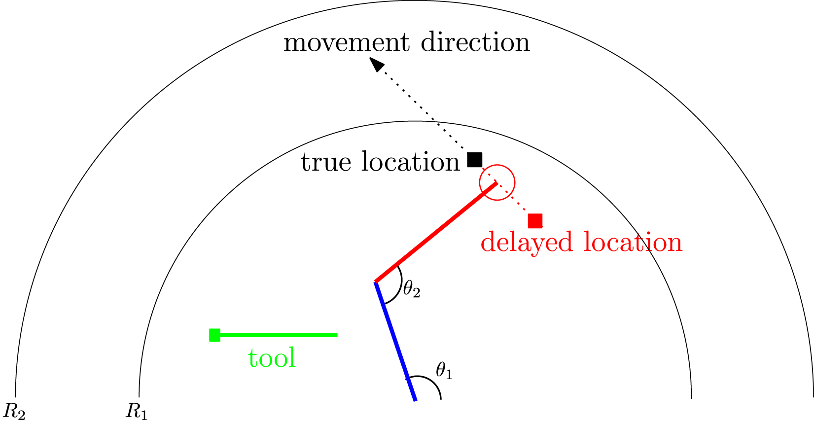

The target was initially placed randomly within one of four regions (upper left, lower left, lower right, upper right), and moved in one of four directions (0^o, 45^o, 135⁰, and 180^o, respectively). The target was moved for 500 simulations steps in the beginning (which was the amount of delay), before the controller can start movement.

Task 2: Reaching Task with Input-Blanking

Task two is mostly similar to task 1, except that there is no delay in the input for the target object, but the target can become invisible depending on the distance between the end-effector of the stick arm and the target object. Figure 7 shows the setup.

Figure 7.

Task 2: Reaching Task With Input Blank-Out. The Task is Mostly the Same as Task 1, but There is No Delay and the Target Object (■) May Become Invisible (□) to the Agent when It is Within the Visibility Distance Threshold (VT)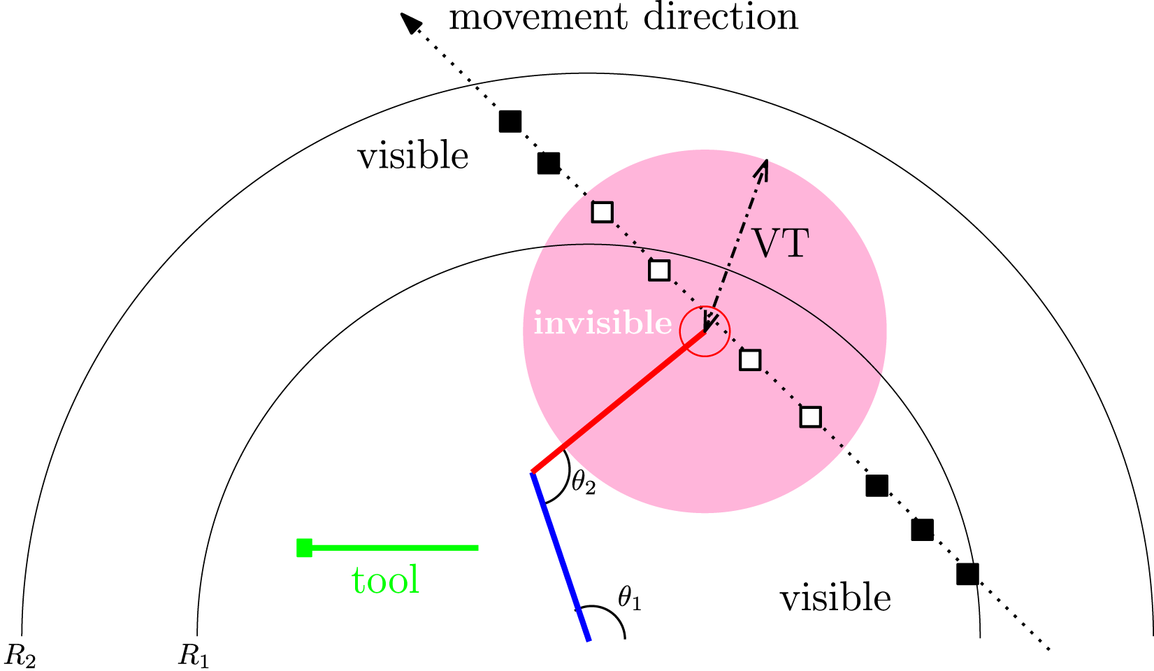

The visibility threshold (VT), a length measure, determined when the target is invisible (the “blank-out”). As shown in Figure 7, the target becomes invisible when it is within this distance from the hand (=VT), and when the target is outside this range, it becomes visible. How long the target is visible or blanked out is dynamically modulated by this single task parameter. We evolved and tested the neural network controllers with four VT conditions: 25, 50, 75, and 100. The rational was, with higher VT, more prediction will be necessary for the agent to be successful. In humans, it has been shown that in a virtual 2D pole balancing task, the subjects were able to withstand up to 600 ms of input blank-out in a “prediction mode” Mehta and Schaal (2002).

To simplify the analysis and focus on how the amount of occlusion correlates with predictive potential, we evolved NEAT controllers with the E factor turned on, and compared two conditions: NEAT with (1) recurrent connections allowed (RNN), and (2) only feed-forward connections allowed (FFN). The rationale was that in order to predict, recurrent connections are needed (to maintain memory). Thus, the expected outcome was that when prediction becomes necessary, RNN would outperform FFN.

NEAT Controller

For control of the arm for both tasks, we used NEAT. Figure 8 shows the initial topology of the controller network. The nine inputs and two outputs of the network were as follows.

Figure 8.

Initial NEAT Topology. The Initial NEAT Controller Topology is Shown. Red: Input, Green: Output. Note that There are No Hidden Neurons, since This is the Initial Topology. See Text for Details. (Note: The figure is Presented Mainly to Show the Topology, so the Label in Each Node is Not Important.)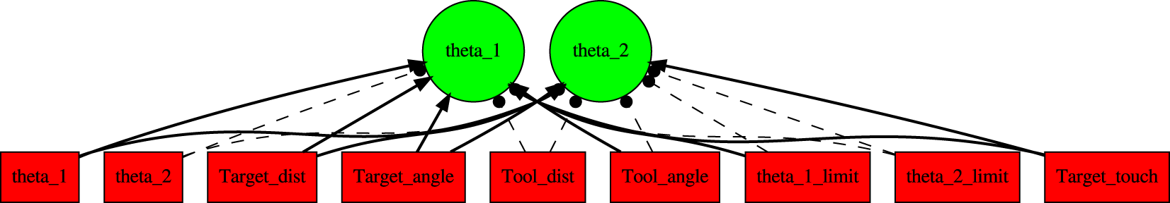

Input: (1) θ₁: joint angle 1, (2) θ₂: joint angle 2, (3) target_dist: distance between hand and delayed target, (4) target_angle angle from hand to delayed target, (5) tool_dist distance between hand and tool handle (not delayed, since the tool is static), (6) tool_angle angle from hand to tool handle, (7) θ_1limit: triggered when joint one limit is reached, (8) θ_2limit: triggered when joint two limit is reached, (9) target_touch: tactile sensor triggered when hand touches the true target.

Output: (1) θ₁: joint angle one adjustment, (2) θ₂: joint angle two adjustment. The adjustments were limited to −1.5^o ≤ θ_i ≤ 1.5^o.

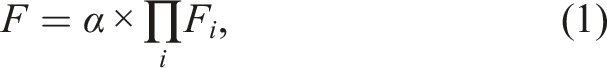
Fitness

We tested a combination of different fitness factors, each scaled between 0.0 and 1.0, and the factors multiplied, as shown below (see the Appendix for details):

F = α \times \prod_{i} F_{i},

(1)

where α is a product of common factors used in all experimental conditions, and ∏_iF_i a product of the fitness factors that are to be compared. The common factor α is defined as α = D × N × C, where D is based on the mean square distance between the true target and the hand location (1 - this quantity), N is the average number of abrupt change of direction to discourage oscillating behavior (1 - this quantity), and C is the total hit count in each behavioral attempt. The main factors we compared were F_i ∈ {E, R, T}, where E is the energy factor (1 - normalized total hand travel distance), R the predictive reach factor (number of five or more consecutive hits), and T the tool factor (tool pick up). In our case, we tested these factor combinations: R, RT, ER, and ERT.

Performance Metrics

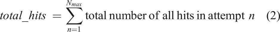
Other than the fitness, each individual was tested in multiple random behavioral attempts (N_max = 100) to measure the performance.

The first metric is the total number of “hits” (touching the target) in each behavioral attempt. (Note that all attempts were 5,000 steps. Also, the maximum value of total hits in each attempt depends on the relative position of the randomly initialized hand, tool, and target positions.) Although this is a good general metric, it does not measure the predictive capability.

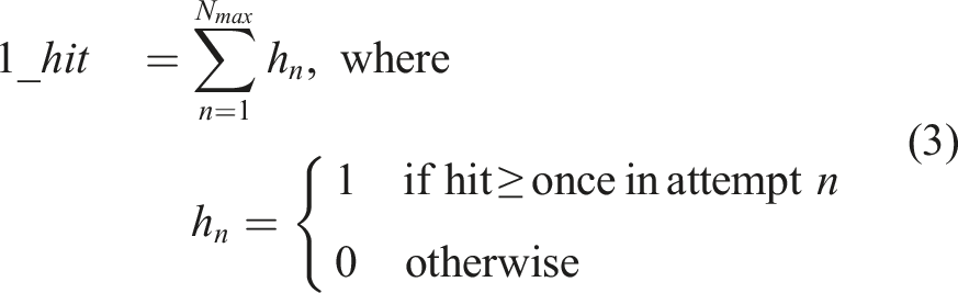
t o t a l_h i t s = \sum_{n = 1}^{N_{\max}} total number of all hits in attempt n

(2)

Metric 1_hit measures the number of attempts in which the agent had reached the target at least once. The 1_hit is computed with equation (3). While this metric is standardized and can show the effectiveness of a network, it cannot distinguish between an accidental hit versus predictive reach.

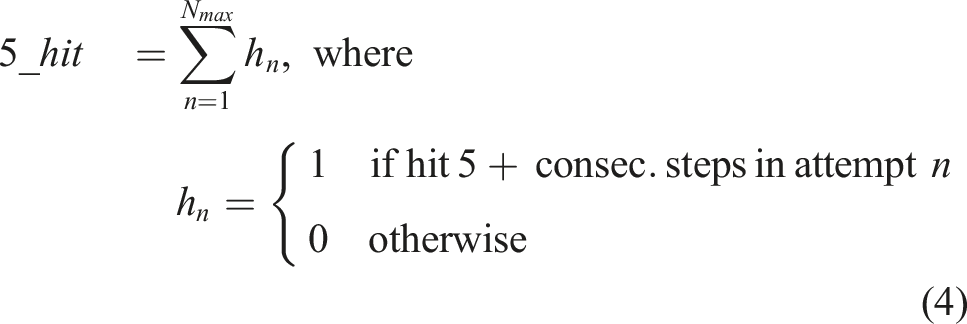
\begin{align} 1_h i t & = \sum_{n = 1}^{N_{\max}} h_{n}, where \\ h_{n} = \{\begin{cases} 1 & if hit \geq once in attempt n \\ 0 & otherwise \end{cases} \end{align}

(3)

Hence, we also introduce the 5_hit metric (equation (4)) which counts the number of attempts in which the agent had reached the target at least five consecutive time steps (a different value may also be used, e.g., 10). This is to ensure that the reach of a target was intentional and therefore is used as our main metric to measure the predictive capabilities of the agents.

\begin{align} 5_h i t & = \sum_{n = 1}^{N_{\max}} h_{n}, where \\ h_{n} = \{\begin{cases} 1 & if hit 5 + consec. steps in attempt n \\ 0 & otherwise \end{cases} \end{align}

(4)

All the metrics mentioned above apart from the fitness scores, act as a standard metric to compare the successes of different agents. They share common extremes ([0, 500,000] for the number of reaches and [0, 100] for 1_hit or 5_hit) and are computed using the same equations resulting in standardized scores.

Task 1: Experiments and Results

Each of the four fitness types (R, RT, ER, ERT) was evolved for 150 generations.

Population Average over Generations

Figure 9 shows the population average of the fitness and the number of reaches over the generations. We find that the ER factor combination significantly outperforms the others (note that in this case, the evolutionary “trial” ended early, since it exceeded the preset fitness threshold).

Figure 9.

Task 1. Population Average of Fitness and Total Number of Hits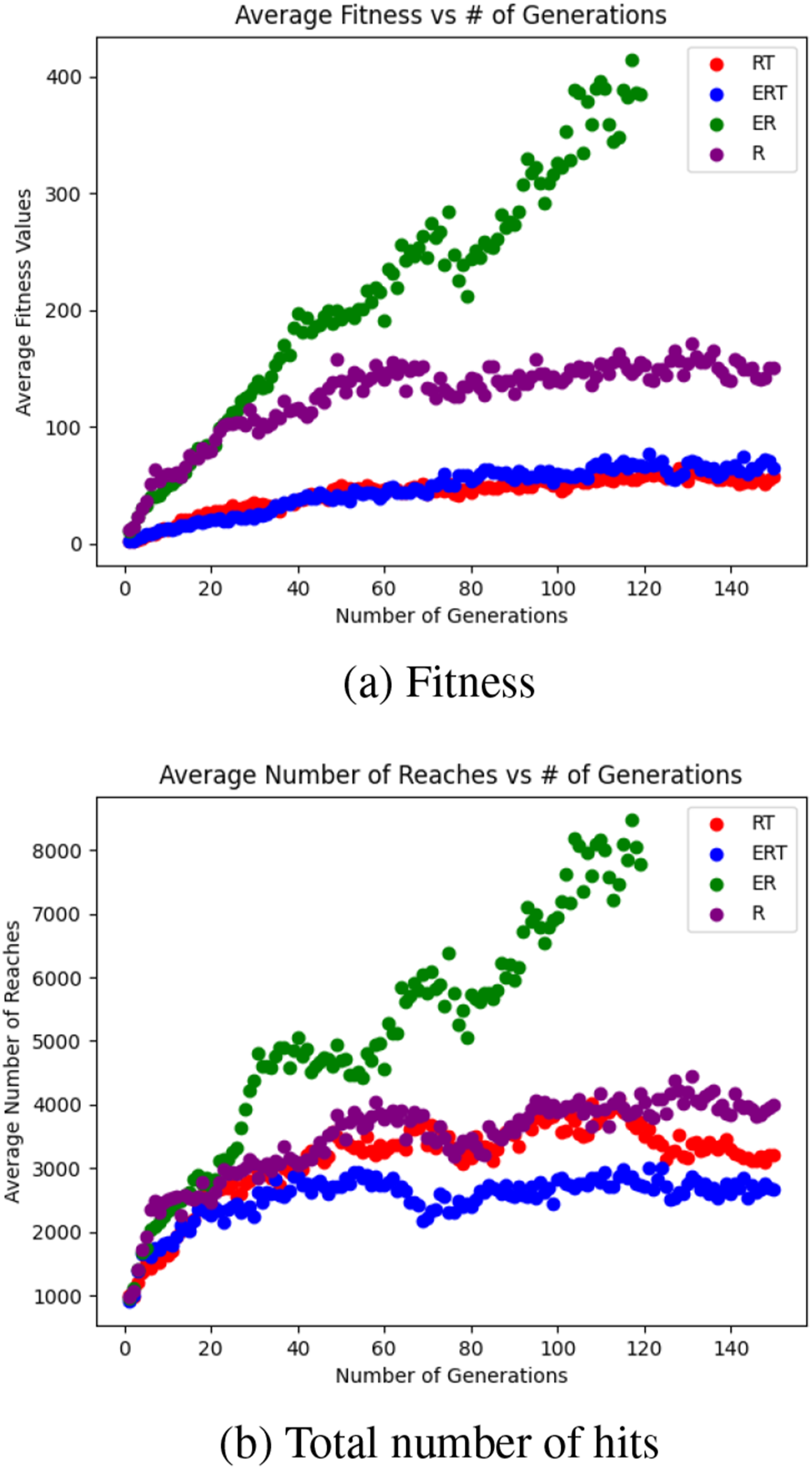

Performance of Best Individuals

Next, we tested the best individuals for each fitness type, using the 1_hit and 5_hit metric (note that E is not a good metric due to trivial cases: e.g., when the agent did not move). For each individual tested, we ran the individual in a task 100 times (“attempts”), and counted the number of times it was able to hit the target once or five consecutive times, respectively. We repeated n (=31) such “runs” to measure the performance (Figure 10). Note that 1_hit and 5_hit can be at the most 100 (N_max = 100). For 1_hit, the results are mixed (Figure 10(A)). ERT shows the best performance, followed by R, ER, then RT. Thus, there is no clear difference between (R, RT) versus (ER, ERT). However, Figure 10(B) shows that for 5_hit, (ER, ERT) clearly outperforms (R, RT). Furthermore, Figure 10(C) shows that most of the 1_hit events are also 5_hit events for (ER, ERT), showing that most reaching behavior is prediction based. However, this is not the case for the (R, RT) condition, where most reaching behavior is blind waving.

Figure 10.

Task 1. Performance of Best Individuals. The (A) 1_hit and (B) 5_hit Results are Shown for the Four Fitness Types. (C) Compares (A) and (B) in a Single Plot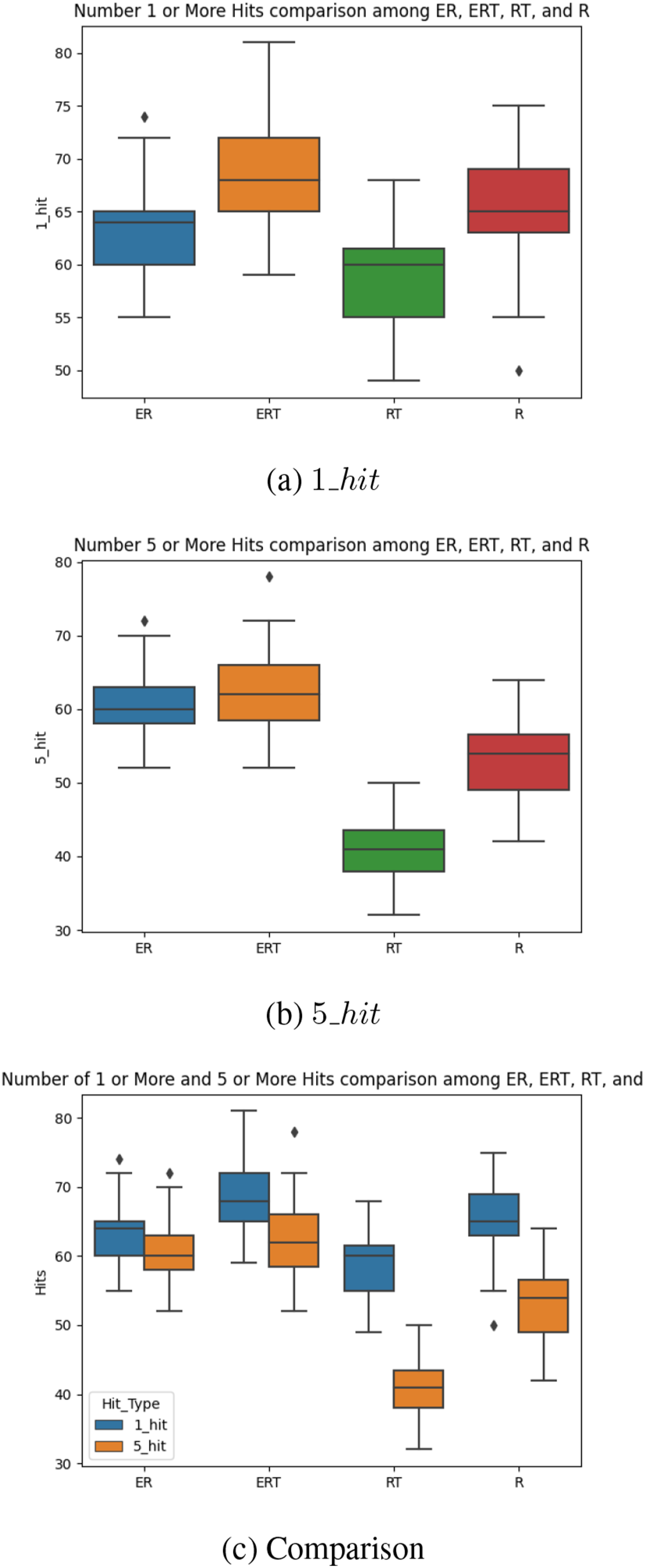

Considering that 5_hit is an indicator of predictive behavior (continuously and intentionally tracking the true target location, rather than randomly waving to hit the target by luck), we can conclude that the fitness types that include the Energy factor facilitates the emergence of predictive behavior.

Behavior

Observing the behavior can provide some insights on the relevance of our 1_hit and 5_hit metrics. Figure 11 show some typical behaviors by fitness type. We plotted the behavior in time lapse (vivid color = most recent frame). We can also see the target’s moving direction (black = true target, red = delayed target): For example, in Figure 11(B), the target is moving from lower left to upper right. For each fitness type, representative behavior that exhibit predictive property (a through d) and those that do not (e through h) are shown. For the top row (predictive), we see that the hand dwells close to the true target location (black square), ahead of the delayed target (red square). This kind of behavior may not be possible without some form of prediction, and may score high on the 5_hit criterion. For the bottom row (non-predictive), the hand makes broad sweeping gestures. This could lead to a high 1_hit score, but a low 5_hit score. With this, we can view the results in Figure 10(C) in a new light: The fitness types that involve the Energy factor may be exhibiting predictive behavior, while those that do not are merely successful in reaching the target through undirected broad sweeping behavior.

Figure 11.

Task 1. Representative Behaviors. Time Lapse of Representative Behaviors are Shown (Vivid Color = Most Recent Frame). Black Square: True Target. Red Square: Delayed Input. Top Row (A ∼D): Predictive Behavior. Bottom Row (E ∼H): Non-predictive Behavior. Note that in (G) and (H), the Tool is Picked up, so the Reach is Extended. See Text for Details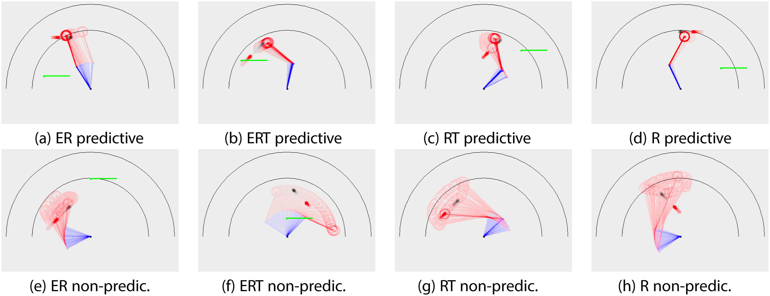

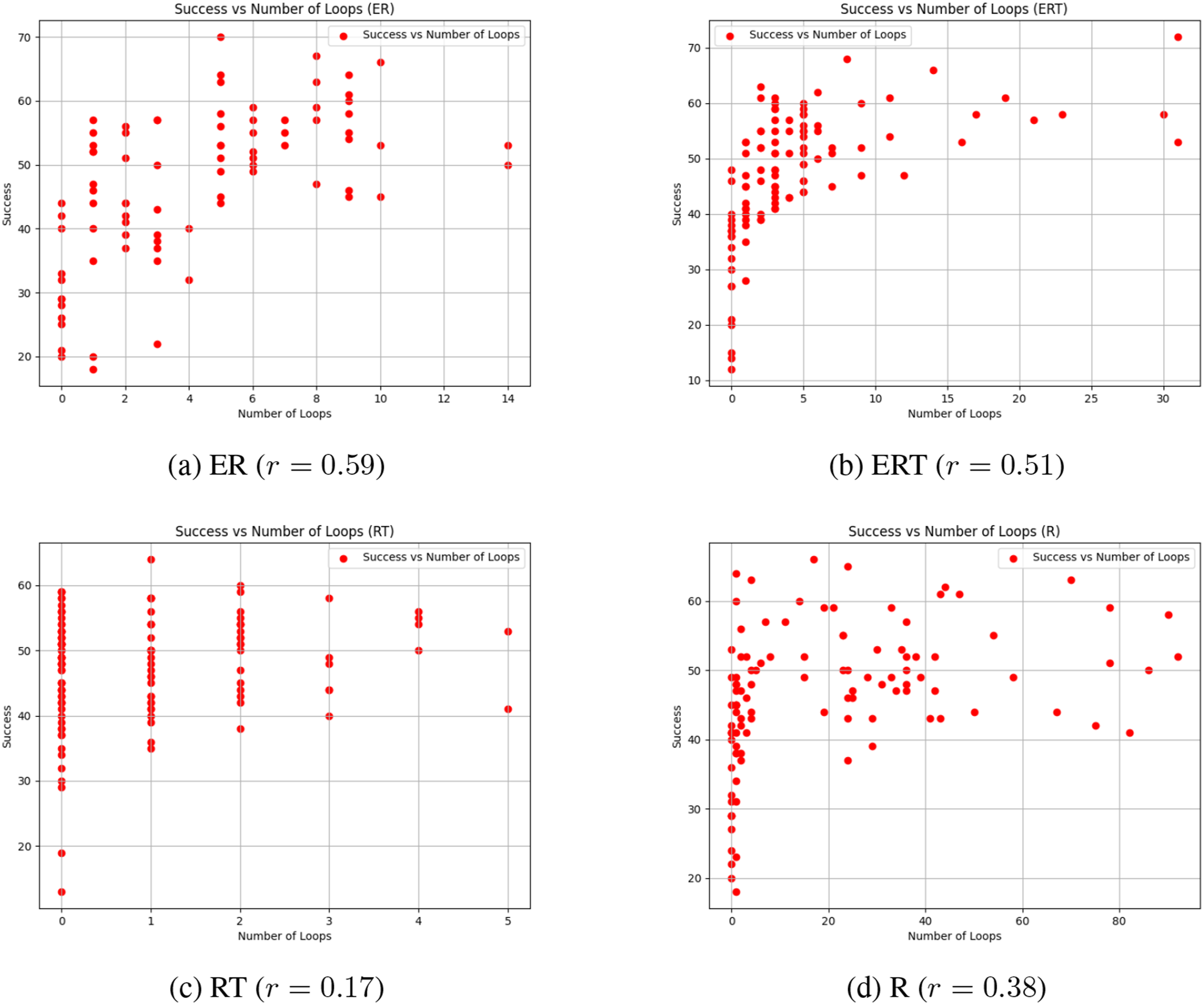
Network Topology

The evolved network topology also gave us further insights on how different fitness types shaped the controller’s behavior (Figure 12). At first glance, there are no distinguishable differences in appearance, other than some having more hidden neurons than others. Further analysis reveals an interesting property. Our previous work on analyzing evolved network topology showed a positive correlation between the number of loops and the performance Li et al. (2015). We conducted the same kind of analysis, by counting the number of simple cycles in the evolved network (we used NetworkX for this Hagberg and Conway (2020)). The results are shown in Figure 13. Interestingly, for the fitness types that include the Energy factor (ER, ERT), the number of loops are strongly correlated with the success rate (r = 0.59 and 0.51, respectively). However, for those without the Energy factor (RT, R), the correlation is weak (r = 0.17 and 0.38, respectively). These results suggest that the recurrent loops in the networks evolved with the energy constraints may be supporting predictive function better than those without. How these loops contribute to prediction need to be investigated (for initial attempts, see lesion studies in Kang and Anand (2023)).

Figure 12.

Task 1. Typical Evolved Topologies. Typical Evolved Topologies are Shown for the Different Fitness Types. Neurons: Red = Input, Orange = Hidden, Green = Output. Connections: Solid Lines With Arrows = Excitatory, Dashed Lines With Discs = Inhibitory

Figure 13.

Task 1. Number of Loops vs. Success Rate. The Number of Loops (Simple Cycles in Graph Theory) in an Individual versus Its Success Rate is Plotted. The r Values are the Correlation Coefficients. Each Point Corresponds to One Individual in the Population. We can See that the Correlation is Higher for the Fitness Types that Includes the Energy Factor (ER and ERT), Compared to Those that do Not Include This Factor (RT and R)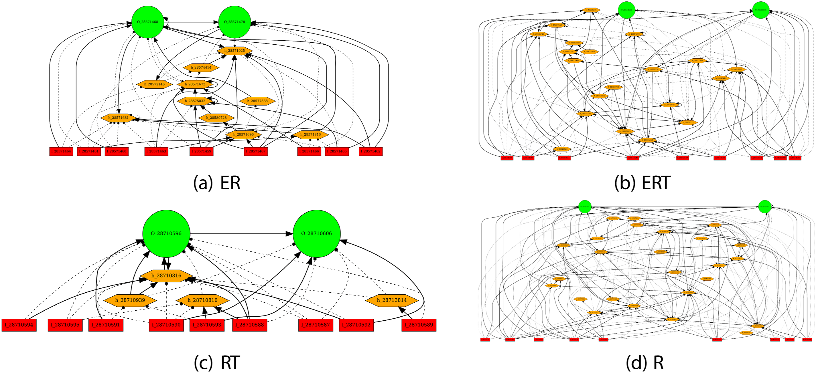

Task 2: Experiments and Results

For Task 2, we evolved NEAT controllers under two different conditions. One with recurrent connections turned on (RNN) and the other with only feed-forward connections (FFN). In all cases, we used the ER fitness factor. Different from Task 1, we evolved the controllers for 200 generations.

Performance of Best Individuals

We tested the best individuals for the two topology types (RNN and FFN) after 200 generations, using the 1_hit and 5_hit metric. The experimental number of trials and statistics gathering were the same as Task 1. The results show that RNNs had better overall performance than FFNs (Figure 14(A)). However, this alone is not enough to answer whether prediction emerged due to input blocking (occlusion). Comparing the 1_hit metric and the 5_hit metric can help answer this question. As we can see in Figure 14(B), the 1_hit performance declines as VT increases from 25 to 100, but there is no significant difference between RNN and FFN. However, for the 5_hit metric, which is an indicator of predictive behavior, the same declining trend is observed, but RNN shows higher performance compared to FFN (VT = 50 and 100, with mixed results for VT = 75). This can be interpreted as a network topology type with more predictive power is able to maintain its performance when faced with tougher occlusion. Thus, given tougher occlusion conditions, networks with more predictive power would evolve.

Figure 14.

Task 2: Performance of Best Individuals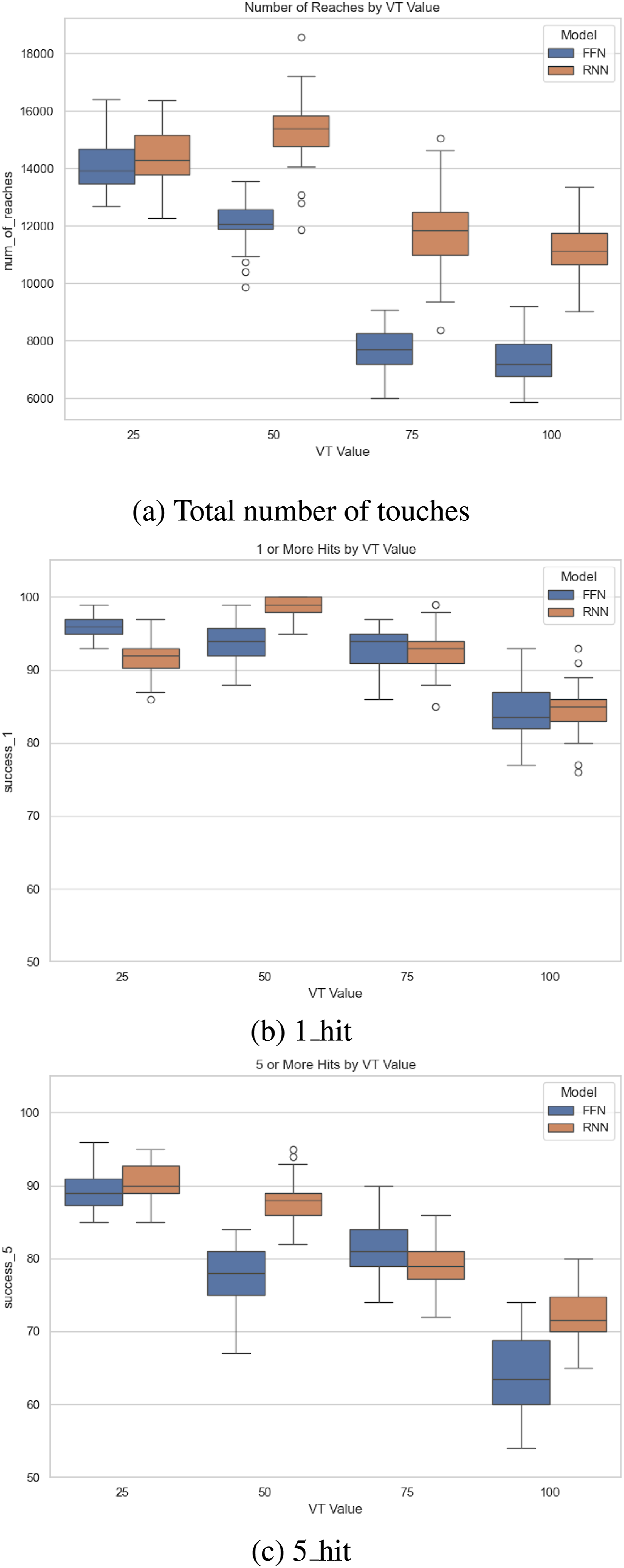

Discussion

The main contribution of this paper is the identification of constraint on energy and occlusion as major factors in the emergence of predictive behavior in the context of evolution. Together with delay and environmental change identified earlier as potential factors in our prior work, we now have a set of four unlikely yet naturally prevalent conditions that could have led to the emergence of prediction.

We have to admit that some of our results are a bit mixed. For example, in Task 2, our prediction metric (5 consecutive hits) showed mixed results for VT = 75, where the feedforward neural network showed better performance than the recurrent network. It is possible that the feedforward controller learned to (1) decide on its initial trajectory while the target is visible and then (2) launch its arm in a ballistic manner and forget about it, thus not requiring continual prediction updates as the input conditions change. However, this is not possible due to two reasons: (1) The feedforward network only receives the present position input and does not receive any velocity information as part of the input, thus it cannot decide on the initial launch of the arm, and (2) since the actuation is kinematic (step by step update of the limb angles) and not dynamic (involving momentum and friction), it cannot launch its arm and forget about it. Further analysis and perhaps a better prediction measure is needed to explain this outcome.

Prediction has become a very hot topic in both neuroscience and artificial intelligence research. However, how prediction evolved and what factors contributed to its emergence have not gained much attention.

Various fields in neuroscience where prediction appears as a key mechanism include sensorimotor control Wolpert and Flanagan (2001), reward prediction Schultz et al. (1997), anticipation Rosen (1985), planning and adaptation, and social interaction Brown and Brüne (2012). In brain theory, prominent models like predictive coding Rao and Ballard (1999) and active inference Adams et al. (2013) all have prediction at its core. Likewise, prediction is playing an increasingly important role in artificial intelligence, especially in foundation models including large language models. Training self-supervised models for vision heavily depend on predicting the next frame in a video from previous frames Nair and Finn (2019), and pretrained transformers also use the next-token prediction task or next sentence prediction task as one of their main tasks Vaswani et al. (2017).

Our approach from an evolutionary point of view, and the identification of key contributing factors can help provide a new perspective to both neuroscience and artificial intelligence research. Instead of just focusing on how the nervous system predicts or how it reduced prediction error, we can consider how different factors may be modulating prediction. In artificial intelligence models, the four factors can be used as novel loss functions, or factors to be included in the task set up or curriculum, to encourage predictive capabilities to develop without explicitly forcing it.

Conclusion

In this paper, we investigated factors contributing to the emergence of predictive behavior in an evolutionary context. We used a reaching task, where in Task 1, reaching the true target with delayed position information required some form of prediction based on the delayed input from the past, and in Task 2, the input was blocked from view (a form of occlusion), again requiring prediction during the occlusion period. In Task 1, we found that the energy factor plays an important role, allowing the evolved controllers to be more successful in the reaching task, and to exhibit more focused predictive reaching behavior. The controllers evolved without the energy factor were moderately successful, but the strategies were mostly based on undirected, systematic sweeping, not indicative of any prediction of the target’s trajectory. Furthermore, we found that structural innovations like recurrent loops in the evolved controllers play a more cohesive role in support of the predictive function, when the energy factor was included. In Task 2, we found that the more severe the occlusion (i.e., the higher the visibility threshold), the controllers with more predictive power (the recurrent neural networks) fared better. These results suggest that energy constraints and occlusion may have served as factors leading to the emergence of prediction through evolution, in addition to delay and environmental change identified in our previous studies.

Footnotes

Acknowledgments

This work is largely based on the undergraduate honor thesis Kang and Anand (2023) and subsequently published conference paper (Figure 6, Figures 8∼13). The paper has been significantly updated, with expanded introduction and background, and new experiments and results. Environment simulation and NEAT configurations were based on Qinbo Li’s code Li et al. (2015), using ANJI James and Tucker (2004). Results from prior works presented in the background section are thanks to Timothy A. Mann and Jaerock Kwon. We would like to thank the anonymous reviewers for Kang et al. (2024) for helping us clarify our points.

ORCID iDs

William Kang

Yoonsuck Choe

Funding

The authors received no financial support for the research, authorship, and/or publication of this article.

Declaration of Conflicting Interests

The authors declared no potential conflicts of interest with respect to the research, authorship, and/or publication of this article.

Author Biographies

William Kang is a computer scientist with a BSc, currently pursuing MSc in Computer Science at Texas A&M University. His work focuses on Computational Neuroscience especially replicating intelligence through Neuroevolution.

Christopher Anand is a computer scientist with a Bachelor of Science in Computer Science and is currently pursuing a Master of Science in Computer Science at Texas A&M University. He is interested in the study of the evolution/emergence of prediction and decision-making behaviors in foraging agents.

Jin Hyun Park is a computer scientist with a BSc in Computer Science and is currently pursuing a PhD in Computer Science and Engineering at Texas A&M University, with a specific focus on computational neuroscience. He is interested in the study of biological and computational vision and the evolution/emergence of prediction.

Yoonsuck Choe is a professor of Computer Science and Engineering at Texas A&M University. His research interests are broadly in neural networks, neuroevolution, and computational neuroscience. He is especially interested in the temporal aspects of brain function (delay, internal brain dynamics, prediction, consciousness), sensorimotor learning and grounding (visual, tactile, proprioceptive, semantics, meaning), agent-environment interaction (including tool construction and tool use), and evolution of brain structure and function.

Appendix

The fitness factors were computed as follows. All factors were computed from N_max behavioral attempts (=100) using the same individual chromosome, with each attempt running for a maximum of M_max simulation steps. W is the width of the arena (=512 pixels), and L is the initial lead up steps which corresponds to the delay (=500 steps for Task 1, and 0 for Task 2). The factors were D: distance, N: turn, C: total hit count, E: energy, R: predictive reaches, T: tool.

D = 1 - \sum_{n = 1}^{N_{\max}} \sum_{m = 1}^{M_{\max}} {d_{n m}}^{2} / {(W N_{\max} M_{\max})}^{2}

N = 1 - \sum_{n = 1}^{N_{\max}} n_{n} / N_{\max} M_{\max}

C = \sum_{n = 1}^{N_{\max}} c_{n} / N_{\max} M_{\max}

E = 1 - \sum_{n = 1}^{N_{\max}} s e_{n} / N_{\max} (M_{\max} - L)

R = \sum_{n = 1}^{N_{\max}} r_{n} / N_{\max}

T = \sum_{n = 1}^{N_{\max}} t_{n} / N_{\max}

where, in each attempt, d_nm = distance between hand and true target in attempt n at time step m, n_n = number of sharp turns (= reversal of hand movement direction $> 9 0^{o}$ ), c_n = total number of hits, e_n = consumed energy (= cumulated hand travel distance), s = energy scaling factor (=1 for Task one and = 10 for Task 2), r_n = 5_hit, t_n = 1 if tool is held and 0 otherwise.

References

Adams

R. A.

Shipp

Friston

K. J.

(2013). Predictions not commands: Active inference in the motor system. Brain Structure & Function, 218(3), 611–643. https://doi.org/10.1007/s00429-012-0475-5

Brown

E. C.

Brüne

(2012). The role of prediction in social neuroscience. Frontiers in Human Neuroscience, 6, 147. https://doi.org/10.3389/fnhum.2012.00147

Bubic

Von Cramon

D. Y.

Schubotz

R. I.

(2010). Prediction, cognition and the brain. Frontiers in Human Neuroscience, 4, 1094.

Choe

Kwon

Chung

J. R.

(2012). Time, consciousness, and mind uploading. International Journal of Machine Consciousness, 4(01), 257–274. https://doi.org/10.1142/s179384301240015x

Gruau

Whitley

Pyeatt

(1996). A comparison between cellular encoding and direct encoding for genetic neural networks. In Koza

J. R.

Goldberg

D. E.

Fogel

D. B.

Riolo

R. L.

(Eds.), Genetic programming 1996: Proceedings of the first annual conference (pp. 81–89): MIT Press.

Hagberg

Conway

(2020). Networkx: Network analysis with python. https://networkx.github.io

James

Tucker

(2004). ANJI: Another NEAT java implementation.

Kang

Anand

(2023). Emergence of prediction in delayed reaching task through neuroevolution. Engineering honors in computer science and engineering thesis. Texas A&M University.

Kang

Anand

Choe

(2024). The role of energy constraints on the evolution of predictive behavior. In From animals to animats 17. SAB 2025. Lecture notes in computer science (14993, pp. 211–222). https://doi.org/10.1007/978-3-031-71533-4_16

10.

Kashyap

H. J.

Detorakis

Dutt

Krichmar

J. L.

Neftci

(2018). A recurrent neural network based model of predictive smooth pursuit eye movement in Primates. In 2018 international joint conference on neural networks (IJCNN) (pp. 1–8). IEEE.

11.

Korb

K. B.

Brumley

Kopp

(2016). An empirical study of the co-evolution of utility and predictive ability. In 2016 IEEE Congress on Evolutionary Computation (CEC) (pp. 703–710). IEEE.

12.

Kwon

Choe

(2008). Internal state predictability as an evolutionary precursor of self-awareness and agency. In Proceedings of the seventh international conference on development and learning (pp. 109–114). IEEE.

13.

Kwon

Choe

(2009). Facilitating neural dynamics for delay compensation: A road to predictive neural dynamics? Neural Networks: The Official Journal of the International Neural Network Society, 22(3), 267–276. https://doi.org/10.1016/j.neunet.2009.03.011

14.

Yoo

Choe

(2015). Emergence of tool use in an articulated limb controlled by evolved neural circuits. In Proceedings of the international joint conference on neural networks. https://doi.org/10.1109/IJCNN.2015.7280564

15.

Lim

Choe

(2006). Compensating for neural transmission delay using extrapolatory neural activation in evolutionary neural networks. Neural Information Processing–Letters and Reviews, 10, 147–161.

16.

Mann

T. A.

Choe

(2010). Neural conduction delay forces the emergence of predictive function in an evolving simulation. BMC Neuroscience, 11(Suppl 1), P62. Nineteenth Annual Computational Neuroscience Meeting: CNS*2010. https://doi.org/10.1186/1471-2202-11-s1-p62

17.

Mehta

Schaal

(2002). Forward models in visuomotor control. Journal of Neurophysiology, 88(2), 942–953. https://doi.org/10.1152/jn.2002.88.2.942

18.

Nair

Finn

(2019). Hierarchical foresight: Self-supervised learning of long-horizon tasks via visual subgoal generation. arXiv preprint arXiv:1909.05829.

19.

Oudeyer

P. Y.

Smith

L. B.

(2016). How evolution may work through curiosity-driven developmental process. Topics in Cognitive Science, 8(2), 492–502. https://doi.org/10.1111/tops.12196

20.

Rao

R. P. N.

Ballard

D. H.

(1999). Predictive coding in the visual cortex: A functional interpretation of some extra-classical receptive-field effects. Nature Neuroscience, 2(1), 79–87. https://doi.org/10.1038/4580

21.

Rosen

(1985). Anticipatory systems: Philosophical, mathematical and methodological foundations. Pergamon Press.

22.

Schultz

Dayan

Read Montague

(1997). A neural substrate of prediction and reward. Science, 275(5306), 1593–1599. https://doi.org/10.1126/science.275.5306.1593

23.

Shwartz Ziv

LeCun

(2024). To compress or not to compress—Self-supervised learning and information theory: A review. Entropy, 26(3), 252. https://doi.org/10.3390/e26030252

24.

Stachenfeld

K. L.

Botvinick

M. M.

Gershman

S. J.

(2017). The hippocampus as a predictive map. Nature Neuroscience, 20(11), 1643–1653. https://doi.org/10.1038/nn.4650

25.

Stanley

K. O.

Miikkulainen

(2002). Evolving neural networks through augmenting topologies. Evolutionary Computation, 10(2), 99–127. https://doi.org/10.1162/106365602320169811

26.

Sussillo

Abbott

L. F.

(2009). Generating coherent patterns of activity from chaotic neural networks. Neuron, 63(4), 544–557. https://doi.org/10.1016/j.neuron.2009.07.018

27.

Tani

(2016). Exploring robotic minds: Actions, symbols, and consciousness as self-organizing dynamic phenomena. Oxford University Press.

28.

Tjøstheim

T. A.

Stephens

(2022). Intelligence as accurate prediction. Review of Philosophy and Psychology, 13(2), 475–499.

29.

Vaswani

Shazeer

Parmar

Uszkoreit

Jones

Gomez

A. N.

Kaiser

Ł.

Polosukhin

(2017). Attention is all you need. Advances in Neural Information Processing Systems, 30(1), 5999–6009.

30.

Whitley

Dominic

Das

Anderson

C. W.

(1993). Genetic reinforcement learning for neurocontrol problems. Machine Learning, 13(2-3), 259–284. https://doi.org/10.1007/bf00993045

31.

Wolpert

D. M.

Flanagan

J. R.

(2001). Motor prediction. Current Biology: CB, 11(18), R729–R732. https://doi.org/10.1016/s0960-9822(01)00432-8

32.

Yao

(1999). Evolving artificial neural networks. Proceedings of the IEEE, 87(9), 1423–1447. https://doi.org/10.1109/5.784219

33.

Yoo

Kwon

Choe

(2014). Predictable internal brain dynamics in EEG and its relation to conscious states. Frontiers in Neurorobotics, 8(00018), 18. https://doi.org/10.3389/fnbot.2014.00018

Evolutionary Factors Contributing to the Emergence of Prediction

Abstract

Keywords

Introduction

Background

Prior Work: Delay and Environmental Change

Delay

Environmental Change

Related Works on Evolution of Prediction

NeuroEvolution of Augmenting Topologies (NEAT)

Methods

Task 1: Delayed Reaching Task

Task 2: Reaching Task with Input-Blanking

NEAT Controller

Fitness

Performance Metrics

Task 1: Experiments and Results

Population Average over Generations

Performance of Best Individuals

Behavior

Network Topology

Task 2: Experiments and Results

Performance of Best Individuals

Discussion

Conclusion

Footnotes

Acknowledgments

ORCID iDs

Funding

Declaration of Conflicting Interests

Author Biographies

Appendix

References