Sage Journals: Discover world-class research

Abstract

Aggregation, the gathering of individuals into a single group as observed in animals such as birds, bees, and amoeba, is known to provide protection against predators or resistance to adverse environmental conditions for the whole. Cue-based aggregation, where environmental cues determine the location of aggregation, is known to be challenging when the swarm density is low. Here, we propose a novel aggregation method applicable to real robots in low-density swarms. Previously, Landmark-Based Aggregation (LBA) method had used odometric dead-reckoning coupled with visual landmarks and yielded better aggregation in low-density swarms. However, the method’s performance was affected adversely by odometry drift, jeopardizing its application in real-world scenarios. In this article, a novel Reinforcement Learning-based Aggregation method, RLA, is proposed to increase aggregation robustness, thus making aggregation possible for real robots in low-density swarm settings. Systematic experiments conducted in a kinematic-based simulator and on real robots have shown that the RLA method yielded larger aggregates, is more robust to odometry noise than the LBA method, and adapts better to environmental changes while not being sensitive to parameter tuning, making it better deployable under real-world conditions.

Keywords

Swarm robotics aggregation reinforcement learning bio-inspired

1. Introduction

Aggregation, defined as the gathering of individuals into a single group, is beneficial for the survival of animals since it provides protection against predators (Camazine et al., 2003; Grünbaum & Okubo, 1994) and increases resistance to adverse environmental conditions (Krause et al., 2002; Rappel et al., 1999). It is often regarded as a prerequisite for most cooperative behaviors in swarm systems, hence poses a fundamental challenge toward deploying swarm robotic systems in real-world scenarios.

Aggregation behaviors fall into two main categories: self-organized and cue-based. In self-organized aggregation, the location of the aggregate is independent of the environment, as observed in the murmuration of starlings (Goodenough et al., 2017), flocking of birds (Halloy et al., 2007), and it is triggered and governed by the interaction among the individuals. In cue-based aggregation, however, aggregation is triggered by an external environmental cue, such as locations with optimal temperatures within the hive of honeybees (Barmak et al., 2023; Frank et al., 2015).

The development of self-organized and cue-based aggregation behaviors that can be deployed on physical robots is an active line of research (Garnier et al., 2008; Misir & Gökrem, 2021; Na et al., 2021; Schmickl & Hamann, 2011; Sion et al., 2022; Tang et al., 2021). Garnier et al. (2008) modeled a self-organized aggregation behavior of cockroaches and then transferred to a swarm of micro-robots. Inspired by the aggregation behavior of young honey bees (Heran, 1952), a cue-based aggregation method, BEECLUST, was proposed in Schmickl and Hamann (2011). The BEECLUST method imitates the aggregation behavior of honey bees in swarm robots. In this method, a robot moves randomly and stops when it encounters another robot for a particular time. The waiting time depends on the intensity of the cue where robots encountered. It was shown that the BEECLUST method performed well in real-world scenarios such as contamination source detection in extreme environments (Sadeghi Amjadi et al., 2020).

In most studies on cue-based aggregation, the swarm density is chosen high enough to trigger and sustain aggregation. In Arvin et al. (2016), the BEECLUST method was studied under various environmental conditions. Among these factors, swarm density defined as the average number of individuals per unit area, is shown to affect the aggregation performance the most. In high swarm density settings, the probability of robot-to-robot encounters is high enough to support forming and growth of aggregates on the cue. However, in low swarm density settings, robot-to-robot encounter has a low probability; thus, formation and growth of aggregation become a major challenge (Arvin et al., 2016). We aim to overcome this limitation as this would allow implementing, for example, bio-hybrid systems where a few robots interact with the biological agents to influence their behavior (Stefanec et al., 2022). So far, most robot-insect interaction is performed in a centralized way using specially designed manipulators (Rekabi-Bana et al., 2023), which limits the studies to laboratory environments.

An example of a study focused on enhancing aggregation performance is the work conducted by Vardy (2016). In this study, ODOCLUST method was proposed using odometry sensors in the robots. The results showed that the ODOCLUST method outperformed the BEECLUST method. Odometry sensors were also used in a foraging task to boost the performance of the swarm. In Gutiérrez et al. (2010), foraging performance was improved by social odometry in which robots share their odometry data with the other robots locally.

In nature, animals such as honey bees use visual (Collett, 1996) and olfactory landmarks (Reinhard et al., 2004a, 2004b) for navigation in complex environments (Srinivasan, 2010). Robotic systems use landmark-based navigation to move along known landmarks using vision, odometry, and memory-based representations (Kumar et al., 2021; Saleh Teymouri & Bhattacharya, 2021). These systems proved to have better robustness to landmark deficiency, adverse conditions, and environmental change compared to methods based on metric localization and mapping (Furgale & Barfoot, 2010; Halodová et al., 2019; Krajník et al., 2010; Paton et al., 2018). In swarm robotics, such navigation methods were implemented in foraging tasks. As an instance, in Lemmens and Tuyls (2009), an adaptive foraging method was proposed based on landmark-based navigation using RFID tags as landmarks.

In the LBA method (Sadeghi Amjadi et al., 2021), a cue-based aggregation algorithm using landmark-based navigation technique was proposed to increase aggregation performance in low-robot density settings. Despite the increased aggregation performance, the LBA method still heavily depends on odometry for navigation. This dependence is a major drawback since odometry is subject to drift and it is not precise when the robots have to move in uneven terrain, which would limit the use of the LBA in real-world scenarios.

In this article, we propose a new aggregation method, Reinforcement Learning-based Aggregation (RLA) which applies reinforcement learning techniques to choose the optimal action based on the perceived landmarks, removing the dependency on odometry.

The contributions of this article are:

1. A novel reinforcement-learning cue-based aggregation method (RLA) is proposed. To the best of our knowledge, this is the first use of RL for cue-based aggregation in swarm robotics.

2. A cyclical parameter update schedule is proposed to balance exploration-exploitation trade-off of controller update, thereby reducing sensitivity of the performance to the RL parameter choice.

The rest of the article is organized as follows: In Section 2, the BEECLUST method, Landmark-Based Aggregation method, and state-of-the-art on reinforcement learning are discussed. In Section 3, the proposed RLA method and a cyclical parameter update schedule are introduced. In Section 4, the simulation and real-robot experimental setup for evaluating the performance of the proposed method and baselines were introduced. The results of the simulations and real-robot experiments were given and discussed in Section 5. Finally, the conclusion of the work and future works were provided in Section 6.

2. Background

2.1. BEECLUST aggregation

Schmickl and Hamann (2011) modeled cue-based aggregation using three behaviors: (1) move forward, (2) avoid obstacles, (3) wait for w_s. The focal robot moves forward until it detects an object. If the object is an obstacle, the focal robot avoids it and continues its motion. If the object is a robot, the focal robot stops and waits. The waiting time, w_s, is calculated as

w_{s} = w_{\max} \frac{{I_{c}}^{2}}{{I_{c}}^{2} + c},

(1)

where w_max is the maximum waiting time, and c is a positive constant. I_c is the cue intensity. Once the waiting time is over, the focal robot turns θ^°, a random variable with a uniform distribution. The BEECLUST method is shown in Figure 1.

Figure 1.

Flowchart of the BEECLUST method.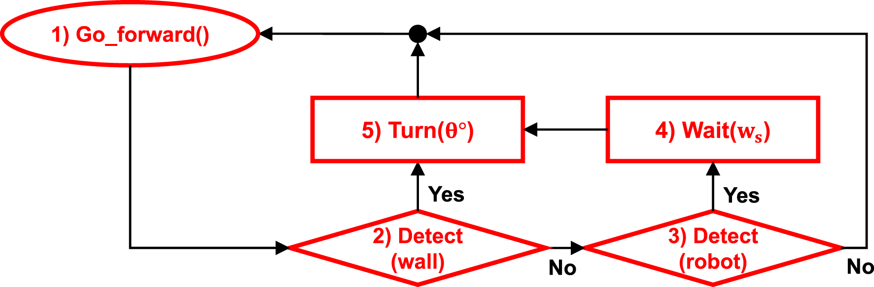

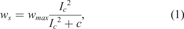
The waiting time is higher inside the cue, where cue intensity is non-zero, causing robots to wait longer there. The higher the cue intensity is, the longer robots wait, and thus, robot-robot encounter probability increases. Consequently, a more stable aggregation is observed in regions with higher cue intensity. Since the BEECLUST method relies on robot-robot encounter probability, in low swarm densities, the probability decreases and affects the aggregation performance adversely.

2.2. Landmark-based aggregation

In the LBA method, when the subject robot detects a landmark for the first time, such as the k^th landmark, it measures its distance d and angle ϕ with respect to the landmark. Then, it calculates its relative position vector $(\vec{R})$ with respect to the landmark as: $\vec{R} = d ∠ ϕ$ .

The robot turns to a random angle and starts to move forward. When it detects an obstacle, it calculates its displacement, ${\vec{S}}_{i}^{k}$ , where i is the index of the displacement vector. The subject robot uses its odometry sensors to measure the distance it traveled and the angle it turned. This process happens each time the robot detects an obstacle. i varies in the range of [1, y], where y indicates the total number of displacement vectors. The process continues until the subject robot encounters another robot. If the encountered robot is inside the region with non-zero cue intensity (referred to as cue), all the displacement vectors are summed to calculate the total displacement vector, ${\vec{S}}_{t o t a l}^{k} .$ Hence, the total displacement vector represents the relative position of the cue with respect to the k^th landmark, ${\vec{S}}_{t o t a l}^{k} = l ∠ ψ$ . When the robot detects the k^th landmark again, it moves towards the cue by following ${\vec{S}}_{t o t a l}^{k} .$ If the robot cannot find the cue after following ${\vec{S}}_{t o t a l}^{k},$ the error variable e^k associated with that vector is incremented. When e^k becomes larger than the error threshold parameter τ_e, ${\vec{S}}_{t o t a l}^{k}$ is reset, and the robot must recalculate ${\vec{S}}_{t o t a l}^{k}$ again.

There are three conditions that a robot cannot find the cue by following the previously calculated ${\vec{S}}_{t o t a l}^{k}$ : (1) The environment might have changed, (2) the location of the cue might have moved, and (3) the accumulated odometry error might be high since the summation of the displacement vectors to calculate the total displacement vector brings vulnerability to odometry noise.

2.3. Reinforcement learning in swarm robotics

As RL gained popularity in solving discrete problems, researchers were motivated to study its capabilities in complex real-world cases. However, in complex and continuous real-world problems, dimensionality and scalability of RL methods impose some disadvantages. Modular RL (Doya et al., 2002) was proposed to decompose a monolithic task into simpler sub-tasks that can be solved in parallel. In Wang et al. (2021), a state evaluation-based weighting method was proposed for determining the mixing weights of two sub-policies. Their experiments on maze tasks showed that the proposed method outperformed other studied approaches and improved the training time. In the context of swarm robots and cooperative learning, two fundamental properties of swarm robotics challenge the cooperative learning scheme, which are: (1) interchangeability of agents and (2) irrelevancy of the exact number of agents. In Hüttenrauch et al. (2019), the mean embedding representation of local observation of each agent is used to enable information exchange among agents despite the aforementioned challenges. Young and La (2020) proposed a cooperative RL scheme to flock the swarm away from the predators. In Franzoni et al. (2020), a swarm of hexagonal robots using the Q-learning scheme was used to interact with humans to maintain social distancing in public areas to avoid the spread of COVID-19 disease. Another study in cooperative reinforcement learning is the GridWorld (Pham et al., 2018) and box pushing (Rahimi et al., 2018). Additionally, a reinforcement learning-based controller for a swarm robotic system is proposed in Na et al. (2022) for autonomous operation of the robots in a real-world scenario.

3. Methodology

3.1. Reinforcement learning-based aggregation

The RLA method is proposed to alleviate susceptibility of LBA method on the odometry noise. The essence of the RLA method is the use of reinforcement learning to choose the best action based on the detected landmark. This choice of action leads to higher robustness to sensory noise. In the RLA method, robots move randomly and aggregate, just as in the BEECLUST method (colored in red) as shown in Figure 2. On top of the BEECLUST method, the RLA method incorporates action selection based on the detected landmark and Q-value updates for the selected action. The swarm aggregation is formulated as an episodic Q-learning problem where each state is considered as a separate bandit problem (Sutton & Barto, 2018).

Figure 2.

Flowchart of the RLA method. Red steps (from 1 to 5) refer to the steps of the BEECLUST method. Snapshots of the kinematic simulation are illustrated in images on the right side. The number specified in the top right corner of the snapshot corresponds to the number of state in the flowchart. (7) A robot detects a landmark and chooses an action. (8) The chosen action of the robot, indicated by the red vector 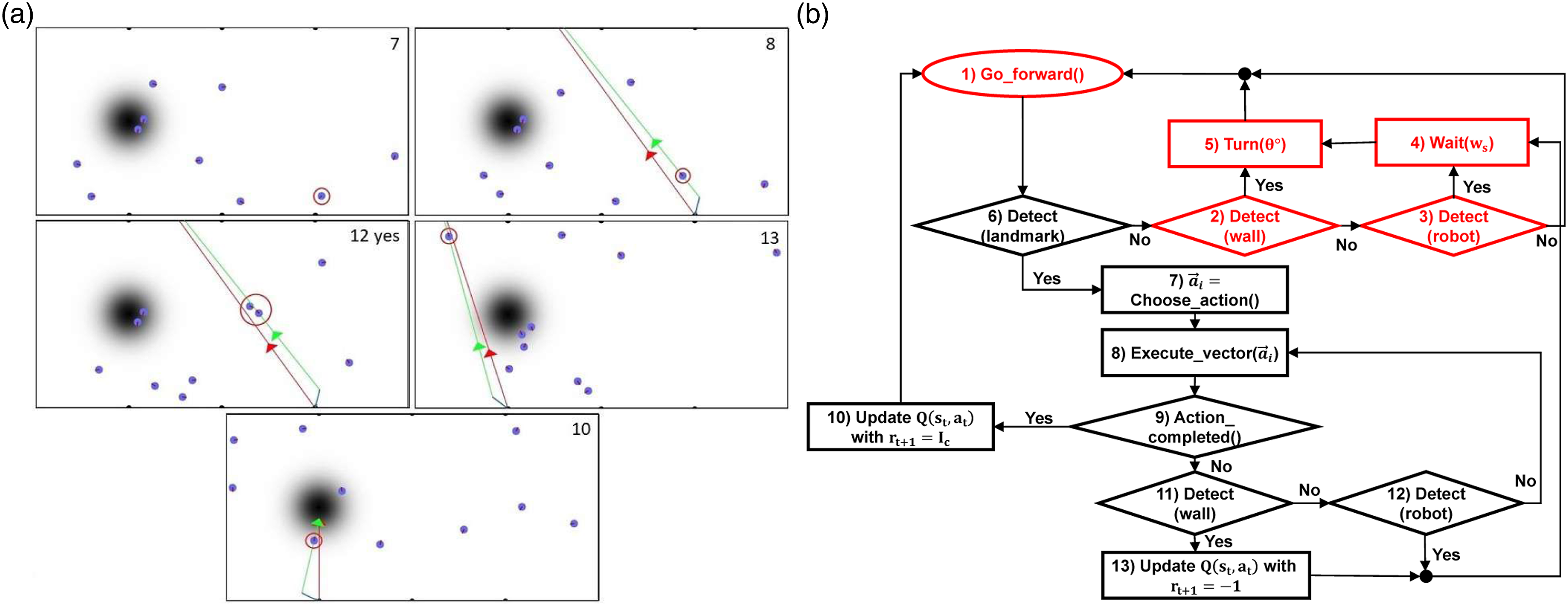${\vec{a}}_{i}$ , is executed. Executing an action stands for following the displacement vector $\vec{T}$ (green vector) which is derived by summing the chosen action $\vec{a_{i}}$ (red vector) and robots’ relative position to landmarks, $\vec{R}$ (blue vector). (9) The Action_completed() function assesses the robot’s ability to effectively track vector $\vec{T}$ and complete the traversal process unhindered by wall collisions or interruptions from other robots. (12) Another robot detected while executing the action. (13) A wall detected while executing an action. (10) Following action led robot to cue and robot receives a positive reward.

When the focal robot detects a landmark (LM), the landmark is set as the state of the focal robot, $S = {L M_{1}, L M_{2}, . ., L M_{m}}$ where m is the total number of landmarks. The focal robot chooses an action from the action space based on its state and the policy function. Based on the detected landmark, the focal robot endeavors to acquire knowledge regarding the action that will guide it from the current landmark state towards the cue. In the rare scenario where multiple landmarks are detected (which is less probable due to the distance between landmarks and robots’ field of view), the focal robot will randomly select one landmark and make a decision on the action to be taken based on that chosen landmark. To incentivize exploration, the ɛ-greedy method is used as the policy function (Watkins & Dayan, 1992).

The action space consists of discrete displacement vectors $A = {{\vec{a}}_{1}, {\vec{a}}_{2}, \dots {\vec{a}}_{n}}$ , where n is the number of actions that a robot can perform in a given state. Each displacement vector starts at the center of a landmark and points to a location inside the arena, including the cue, as shown in Figure 3. The vectors are discretized to reduce complexity and computational cost. Each displacement vector can be written as ${\vec{a}}_{i}^{k} = l ∠ ψ$ , ψ ∈ ⊝, $l \in L$ . Since each displacement vector, ${\vec{a}}_{i}^{k}$ , starts from the center of the k^th landmark, the relative location of the focal robot with respect to the detected landmark $(\vec{R})$ should be added to the displacement vector. By adding this vector, the focal robot reaches the endpoint of the displacement vector by following the target vector $\vec{T}$ calculated as: $\vec{T} = {\vec{a}}_{i}^{k} + \vec{R}$ .

Figure 3.

Action space of a robot in the RLA method. The red vector represents the relative location of the robot with respect to the landmark. Each green vector is the action 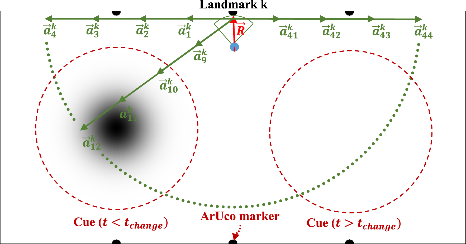$({\vec{a}}_{i}^{k})$ that a robot executes by following $\vec{T} = \vec{R} + {\vec{a}}_{i}^{k}$ , where superscript k represents the k^th landmark and index i ∈ [1, 44] represents the i^th action. The green arc represents the camera field of view of the robot. Red dashed circle on the left and right demonstrates the cue before and after t_change, respectively.

There exist three potential outcomes for the reward received by the focal robot. Upon successfully following target vector $\vec{T}$ without encountering collisions with walls or other robots, the reward corresponds to the intensity of the sensed cue after traversing $\vec{T}$ . If the focal robot fails to reach the cue, a reward of zero (r = 0) is given. In the event of a wall collision during action execution, a reward of r = −1 is given. Moreover, if the focal robot detects the presence of another robot during its action, it ceases to follow the target vector $\vec{T}$ , executes a random turn, and resumes movement within the arena without receiving any reward. Consequently, the reward acquired by the focal robot falls within the range of r ∈ [−1, 255].

After receiving the reward, the focal robot updates its Q-table using the following recursive update rule

Q_{t + 1} (s_{t}, a_{t}) \leftarrow (1 - α) Q_{t} (s_{t}, a_{t}) + α r_{t + 1}

(2)

where α ∈ (0, 1], is the learning rate.

In the BEECLUST method, upon reaching the cue, if a robot collides with another robot, it will wait for a designated duration based on the intensity of the sensed cue at the collision location. In the LBA and RLA methods, extra steps were added on top of the BEECLUST method upon reaching the cue. In the LBA method, in addition to waiting at the cue when encountering another robot, if a robot has previously encountered a landmark before reaching the cue, it will calculate and learn the displacement vector required to navigate from that landmark to the cue. In the RLA method, apart from pausing at the cue when a collision occurs, if a robot reaches cue as a result of executing and action, it will receive a reward based on the sensed cue intensity at the corresponding location.

3.2. Exploration-exploitation dilemma

In order to increase the performance of the RLA method, one of the most important issues is to find the best algorithm for the exploration-exploitation dilemma. In RLA, once a robot detects a landmark, it uses the policy function π_t(s_t) to choose an action. A policy function maps the state space to an action space $π : S \to A$ . Action can be chosen either randomly (exploration) or by selecting the best (exploitation). If an agent always takes random actions, it would explore and learn various possibilities, but it will never use the learned knowledge. On the other hand, if an agent always exploits its knowledge to choose the best action, it will not explore most of the environment’s possibilities, and the chances of received rewards being restricted by local minimum are high. Therefore, a balance is required between exploration and exploitation. This problem is called the exploration-exploitation dilemma. In our case, robots explore environmental possibilities by trying out all possible actions within the action space upon detecting a landmark, encompassing cases where an action leads to a collision with a wall or directs the robot to any position within or outside the cue area. By exploring these diverse possibilities, the robots acquire knowledge regarding which actions are more likely to lead to locations with higher cue intensities. Exploring becomes significantly crucial in dynamic environments since actions after detecting a landmark that lead to the highest intensity of the cue can change.

A simple and effective solution for solving this problem is the ɛ-greedy method (Watkins, 1989) in which the chance of taking a random action is determined by the parameter 0 ≤ ɛ ≤ 1 and the probability of taking a greedy action is 1 − ɛ. In our study, ɛ parameter plays a vital role in the performance of the swarm.

3.2.1. Adaptive ɛ-greedy

In Tokic (2010), an adaptive ɛ-greedy concept called Value-Difference Based Exploration (VDBE) was proposed. In the VDBE approach, an agents’ certainty about the environment is measured by the difference between the value functions of the current and previous steps. Equations (3) and (4) represent the update formula for ɛ in VDBE schedule

f (s_{t}, a_{i}^{k}, σ) = \frac{1 - e^{\frac{- | Q_{t + 1} (s_{t}, a_{i}^{k}) - Q_{t} (s_{t}, a_{i}^{k}) |}{σ}}}{1 + e^{\frac{- | Q_{t + 1} (s_{t}, a_{i}^{k}) - Q_{t} (s_{t}, a_{i}^{k}) |}{σ}}}

(3)

ε_{t + 1} (s_{t}) = δ f (s_{t}, a_{i}^{k}, σ) + (1 - δ) ε_{t} (s_{t})

(4)

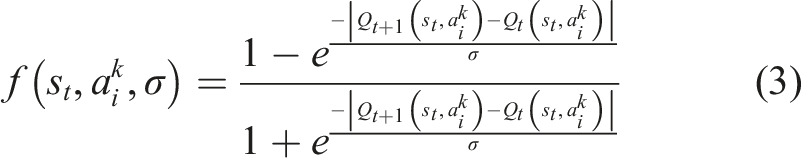
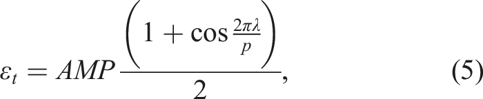
The parameter ɛ is updated using the difference between value functions in two consecutive time steps, $| Q_{t + 1} (s_{t}, a_{i}^{k}) - Q_{t} (s_{t}, a_{i}^{k}) |$ . The parameter δ controls the ɛ rate of change was chosen as the inverse of the number of actions in the current state, $δ = 1 / | A |$ . The inverse sensitivity parameter σ adjusts how sensitive an agent should be to changes in the environment. For the VDBE schedule, σ is the only parameter that needs to be tuned. Higher σ values will act like constant ɛ, which means changes in the environment will not affect ɛ considerably. On the other hand, lower σ values will change ɛ drastically even if a small change happens in the environment. Thus, depending on the conditions of the environment, σ must be tuned to obtain the best performance.

3.3. Proposed ɛ schedule

We propose a new ɛ schedule inspired by the cyclical learning rate changing scheme proposed in Smith (2017). In this schedule, ɛ is changed periodically regardless of the state of the agent

ε_{t} = A M P \frac{(1 + \cos \frac{2 π λ}{p})}{2},

(5)

where ɛ_t is the value of ɛ at time t. and λ is the epoch count which is incremented each time a robot detects a landmark and executes an action. For simplicity, we used cosine function. The parameters amplitude AMP ∈ (0, 1] and period p ∈ (0, ∞) determine how ɛ change in time.

4. Experiments

To evaluate RLA method, experiments on kinematic-based simulator and real-robots were conducted. The experiments were repeated 5 times with randomized initialization conditions.

The learning rate is set to a constant value α = .1; since the environment is non-stationary and noisy, a small, constant value for α will cause slow but guaranteed convergence (Sutton & Barto, 2018).

The performance of aggregation was assessed using the Normalized Aggregation Size (NAS) metric, which is defined as the number of robots inside the cue divided by the population size, NAS ∈ [0, 1].

4.1. Kinematic-based simulator experiments

Kinematic simulation was implemented using Python programming language. Robots were modeled as circles, as shown in Figure 3. The parameters of the robots were chosen such that their size and speed were the same as the Kobot robots (Turgut et al., 2007) used in the real-robot experiments. The radius of the robots were R_r = .06 m, collision detection range was R_col = .06 m with a 360^° collision detection angle. At each time step k, the location of i^th robot is updated according to

[\begin{array}{l} x_{k + 1}^{j} \\ y_{k + 1}^{j} \\ θ_{k + 1}^{j} \end{array}] = [\begin{array}{l} 1 & 0 & 0 & v_{k}^{j} \cos θ_{k}^{j} \\ 0 & 1 & 0 & v_{k}^{j} \sin θ_{k}^{j} \\ 0 & 0 & 1 & ϵ_{k}^{j} \end{array}] [\begin{array}{l} x_{k}^{j} \\ y_{k}^{j} \\ θ_{k}^{j} \\ Δ t \end{array}],

(6)

where

x_{k}^{j}

y_{k}^{j}

, and

θ_{k}^{j}

are the location and orientation of robot,

v_{k}^{j} \in [- 0.14,0.14]

m/s is the forward velocity of a robot, and

ϵ_{k}^{j} \in [- 2 π, 2 π]

rad/s is its angular speed. Δt is taken as .512 s.

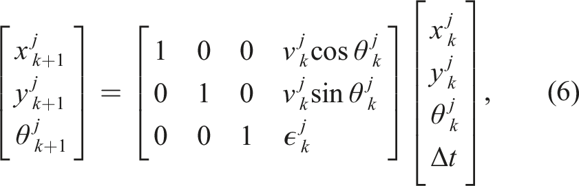
A rectangular arena with dimensions of 2.82 m × 5.65 m was used for all the experiments. The robots were identical and their number was N = 10 in order to create a low-robot density condition. The cue was represented as a dark circle inside the arena with a radius of R_c = 1 m. The intensity of the cue reduces towards its perimeter, and its distribution along its radius was considered to be a 2D Gaussian centered at the center of the cue, as shown in Figure 3. In order to test the performance of the methods in non-stationary environments, the location of the cue was moved during the experiment from (1.41 m, 1.41 m) (the left-hand side of the arena) to (1.41 m, 4.23 m) (the right-hand side of the arena) at time t = t_change.

The duration of each experiment, denoted as t_total, was determined to be sufficiently long for all the methods to reach a steady-state. This decision was made through empirical observation, considering the need for the swarm to achieve a steady-state and maintain it for a certain period. At the same time, it was important to ensure that the experiments could be completed within a reasonable timeframe. The location of the cue was changed at half time of the whole experiment duration, t_change = t_total/2. For the LBA method, the error threshold parameter was τ_e = 4, since this choice has the benefit of both good adaptation characteristics for non-stationary environments and robustness to odometry noise as discussed in Sadeghi Amjadi et al. (2021).

In order to study the robustness of the LBA method to odometry noise, noise was added to the angle of the total displacement as described in Sadeghi Amjadi et al. (2021). If the actual angle of the displacement vector is $β_{i}^{k}$ , the noisy angle ${\tilde{β}}_{i}^{k}$ is calculated using

{\tilde{β}}_{i}^{k} = β_{i}^{k} + σ_{n} η_{i}^{k},

(7)

where η is a uniformly distributed random variable between −1 ≤ η ≤ 1. σ_n is the strength of noise in the range of [0^°, 180^°]. The reason that noise was only added to the angle of the displacement vectors is that in the LBA method when a robot detects the k^th landmark, it moves along the displacement vector,

{\vec{S}}_{t o t a l}^{k}

, until it detects an obstacle or another robot. Therefore, the length of the vector is not important.

In the arena, three landmarks were placed at equal distances from each other on each side of the arena, making a total of six landmarks, m = 6, as shown in Figure 3. It was assumed that robots could detect landmarks up to .5 m.

The action space,

A

, was designed to have n = 44 displacement vectors. The length and angle of action vectors are discretized as

l \in L = {1.25,2.5,3.75,5}

m and ψ ∈ ⊝ = {0^°, 18^°, 36^°, …, 180^°}. Angles are measured in the right-handed body-fixed coordinate frame of each landmark, such that the orthogonal vector towards a landmark is ψ = 90^°. The parameters used in the kinematic simulation are shown in Table 1.

Table 1.

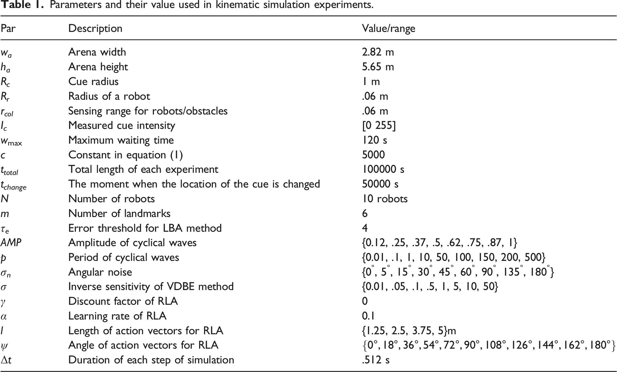
Parameters and their value used in kinematic simulation experiments.

Par	Description	Value/range
w _a	Arena width	2.82 m
h _a	Arena height	5.65 m
R _c	Cue radius	1 m
R _r	Radius of a robot	.06 m
r _col	Sensing range for robots/obstacles	.06 m
I _c	Measured cue intensity	[0 255]
w _max	Maximum waiting time	120 s
c	Constant in equation (1)	5000
t _total	Total length of each experiment	100000 s
t _change	The moment when the location of the cue is changed	50000 s
N	Number of robots	10 robots
m	Number of landmarks	6
τ _e	Error threshold for LBA method	4
AMP	Amplitude of cyclical waves	{0.12, .25, .37, .5, .62, .75, .87, 1}
p	Period of cyclical waves	{0.01, .1, 1, 10, 50, 100, 150, 200, 500}
σ _n	Angular noise	{0^°, 5^°, 15^°, 30^°, 45^°, 60^°, 90^°, 135^°, 180^°}
σ	Inverse sensitivity of VDBE method	{0.01, .05, .1, .5, 1, 5, 10, 50}
γ	Discount factor of RLA	0
α	Learning rate of RLA	0.1
l	Length of action vectors for RLA	{1.25, 2.5, 3.75, 5}m
ψ	Angle of action vectors for RLA	${0 °, 18 °, 36 °, 54 °, 72 °, 90 °, 108 °, 126 °, 144 °, 162 °, 180 °}$
Δt	Duration of each step of simulation	.512 s

The following three experiments were performed using the kinematic-based simulator:

• Environment Experiment: In this experiment, the BEECLUST, LBA, and RLA (with VDBE and cyclical ɛ schedules) methods were compared. First, this comparison was made without considering any odometry noise. Then, a nominal noise, σ_n = 15^°, was added to displacement vectors based on equation (7). Moreover, the performance of the methods was evaluated in non-stationary environments. Time evolution of NAS values was plotted.

• Noise Experiment: In this experiment, the robustness of the methods against noise was studied. Noise was added using equation (7) with σ_n ∈ {0^°, 5^°, 15^°, 30^°, 45^°, 60^°, 90^°, 135^°, 180^°}. For this experiment, the steady-state NAS values were plotted for the sake of clarity of the plots, which were calculated by using the last 100 NAS values of each run.

• Parameter Sensitivity Experiment: In this experiment, the sensitivity of ɛ schedules for the RLA method to different parameter values was evaluated. Two schedules were implemented for ɛ, which are VDBE and cyclical schedule. VDBE schedule has only one free parameter σ, whereas the cyclical schedule has two free parameters p and AMP. As in the previous test case, steady-state NAS values were considered. For backing up the statements made in this experiment, the average of rewards that the swarm has received and the change of the ɛ parameter were also plotted over time.

4.2. Real-robot experiment

In real-robot experiments, the Kobot V2 robots (Turgut et al., 2007), a differentially driven CD-sized mobile robot designed specifically for swarm robotic research, Figure 4, was used.

Figure 4.

Kobot swarm robotic platform. The diameter and height of a Kobot are 12 cm and 11 cm, respectively.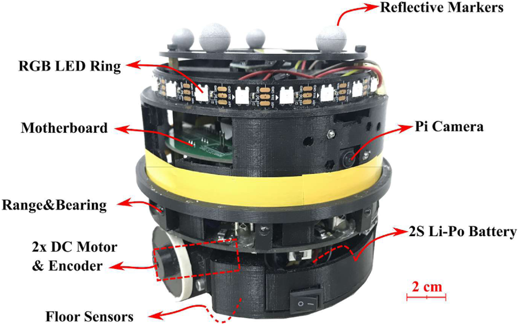

The ArUco markers (Garrido-Jurado et al., 2014) was chosen as the landmarks due to their simplicity, relatively low computational requirements, robustness to occlusion, and low rate of false positive detection. The OpenCV library (Baggio et al., 2012) was used to calculate the position and orientation of the ArUco markers in five steps: (1) Image segmentation: the most distinguishable edges are extracted. (2) Contour filtering: a counter extraction method (Suzuki et al., 1985) followed by a polygonal approximation (Douglas & Peucker, 1973) is applied. (3) Marker code extraction: the internal code of detected regions is analyzed to obtain their internal code. (4) Marker identification and error correction: the environment is distinguished from markers. (5) Corner refinement and pose estimation.

Detection of ArUco markers was implemented on Raspberry Pi 3B + running Raspbian OS and ROS Melodic (Quigley et al., 2009) with the Raspberry Pi Camera v2.1. Kobot robots can detect markers with a .05 m edge up to 2 m distance and from skew angles up to 80^°. Nevertheless, detection distance was limited to .5 m to be consistent with the simulations and to avoid detecting landmarks from inside the cue.

Four IR sensors were placed at the bottom of the robot to sense the cue intensity on the floor. IR sensors were calibrated to read 0 from the lowest intensity zone (the carpet on the floor) and 255 from the highest intensity zone (the brightest zone at the center of the cue). Four readings were taken at each location and averaged to compensate for the tilt of the robot and for the non-uniformity of the floor. Optical encoders coupled to the two DC motors were used as odometry sensors. Obstacle and robot detection were performed using the legacy range and bearing system that has 8 modulated IR sensors. The range and bearing system has a range of 20 cm, and it is able to distinguish robots from obstacles.

During the experiments, all robots relied on on-board sensory data and computational resources, and there was no communication between the robots. Only high-level commands such as experiment start, end, and debugging messages were transferred to Kobot robots from the main computer. In terms of battery and power source, 2S (7.4 V Nominal) Li-Po 1300 mAh battery was used in the robots. With this battery, Kobot robots could run up to 2 hours with a CPU load of 50% of the main controller.

In order to calculate the NAS values during the experiment, 2-D poses of each robot were tracked using OptiTrack motion capture system (OptiTrack, US) with 8 USB cameras. The pose information from the camera array was transferred to the main computer running ROS Melodic for real-time NAS calculation and monitoring the current state of the experiment. By observing the real-time NAS value during the experiment, the time at which NAS reached a steady-state value was noted, and the experiment duration was set accordingly. The setup for real-robot experiment is shown in Figure 5.

Figure 5.

Real-robot experiment setup. Position of each robot is calculated by eight pose cameras (Optitrack) located around the arena. Then, this data is sent to the main computer in order to calculate the number of robots inside the cue for derivation of NAS performance. A webcam is also located in the arena to record the experiments for documentation purposes. Kobots are utilized with on-board camera to detect the ArUco marker, that is, landmarks.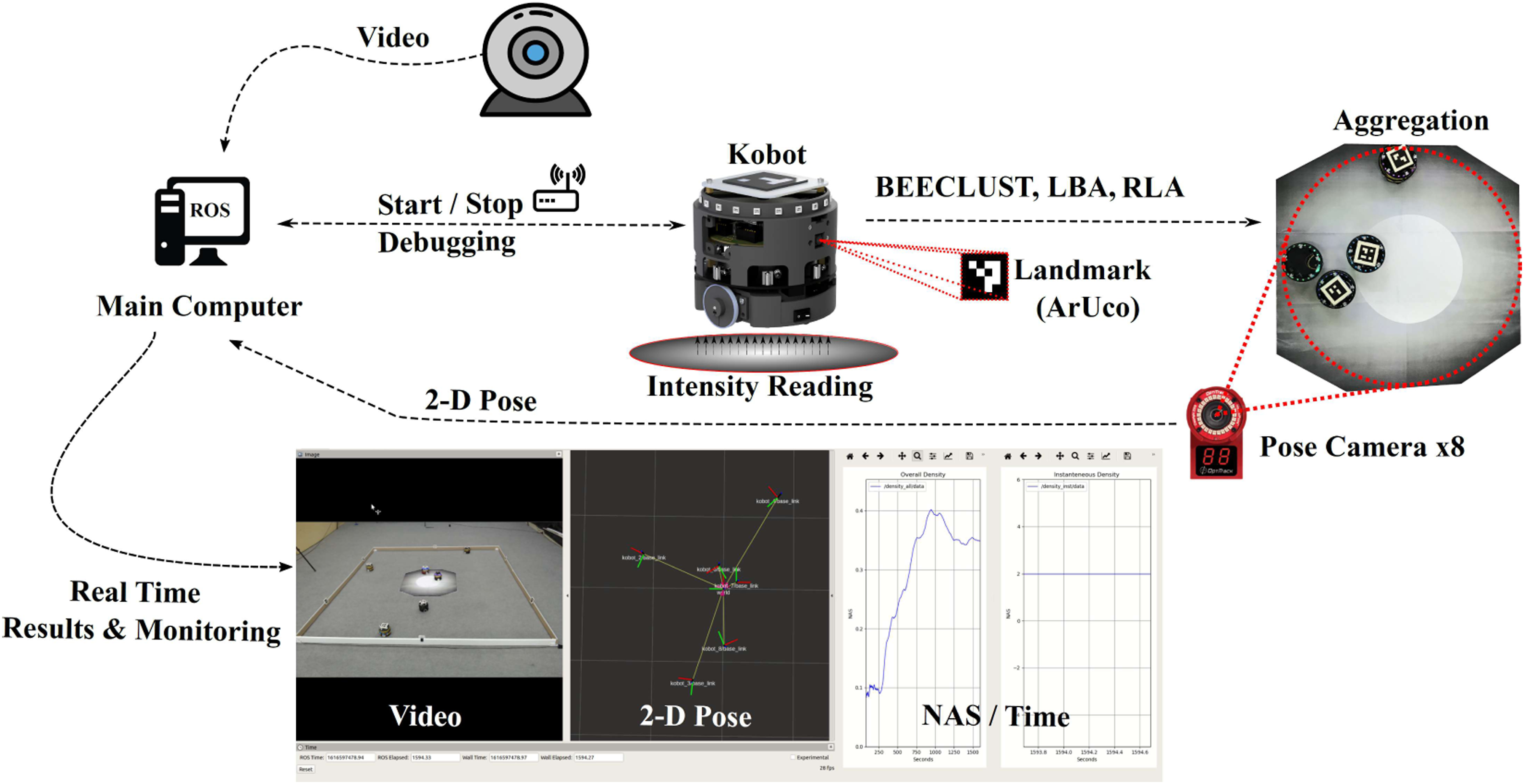

The experimental setup consisted of a rectangular arena with six landmarks placed on the two sides of the rectangle and a circular cue with a white gradient indicating higher intensity regions, as shown in Figure 6. The maximum speed of robots was set to be v^j = .14 m·s⁻¹. Real-robot experiments were conducted in two different swarm sizes, N = {4, 6} robots, to study the performance of the methods in two different population densities. The arena for N = 4 robots case was a 2.8 m × 1.4 m with a cue radius of .3 m. For the N = 6 robots case, arena was 2.8 m × 2.8 m with a cue radius of .45 m. The arena for N = 6 robots setup is illustrated in Figure 6. For all three methods, the maximum waiting time was set to be w_max = 90 s. The reason for choosing this waiting time is that a lower waiting time will hamper the aggregation of robots, and no proper aggregation would be formed. On the other hand, time limitation forced by battery life of robots demands a low waiting time. Otherwise, robots would be waiting most of the time inside the cue until their battery dies. Through empirical investigation, we determined that a suitable compromise for the maximum waiting time is 90 s, considering both sufficient lengths of battery life and aggregation performance. Table 2 shows the parameters used in the real-robot experiment.

Figure 6.

Arena setup for N = 6 robots experiment. A 2.8 m × 2.8 m rectangular arena with six landmarks is surrounded by eight pose cameras (Optitrack) which are used for evaluating the number of robots inside the cue. Robots are calibrated in a way that the grey color of carpet is read as zero cue intensity.

Table 2.

Parameters and their value used in real robot experiments.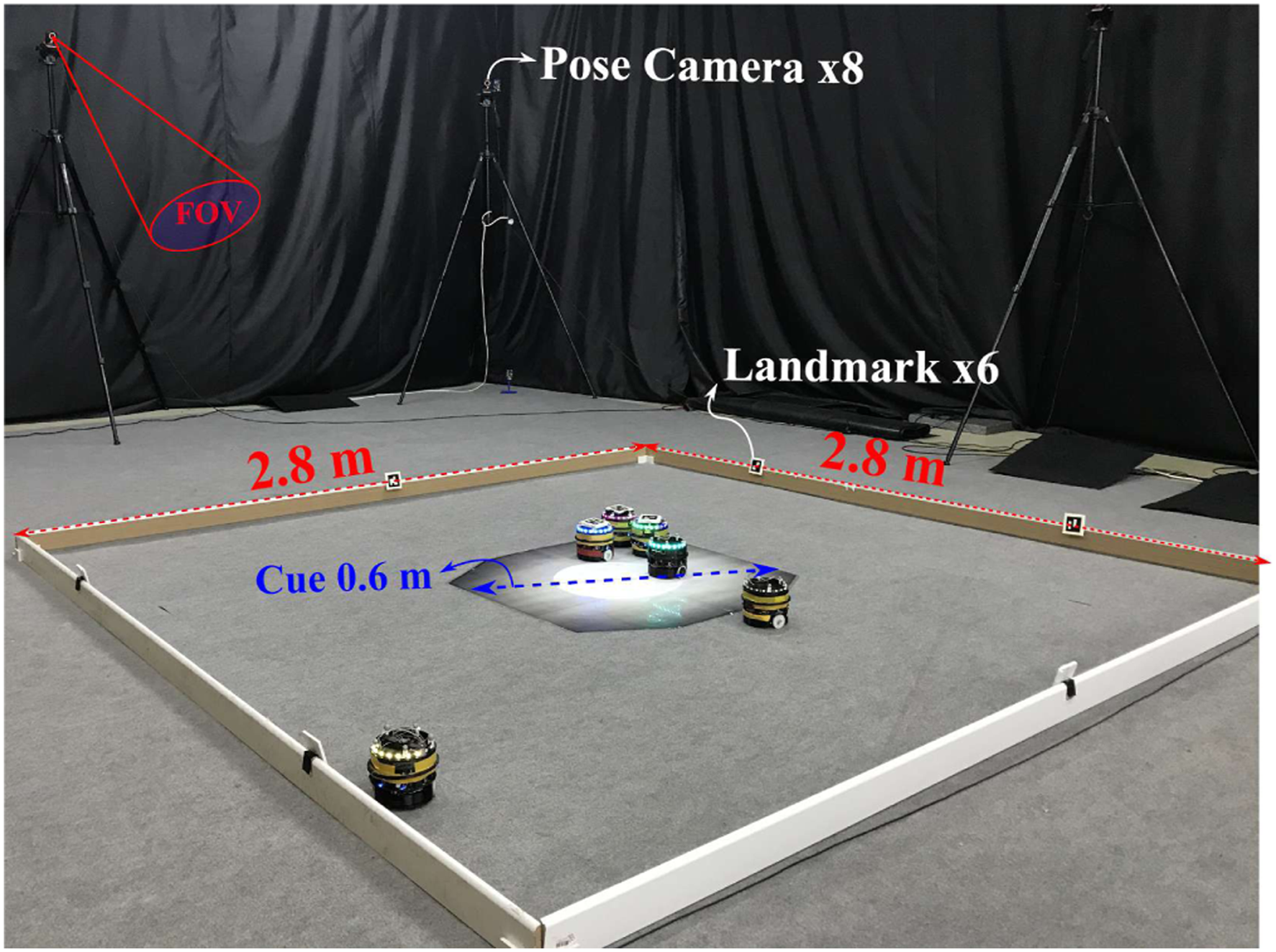

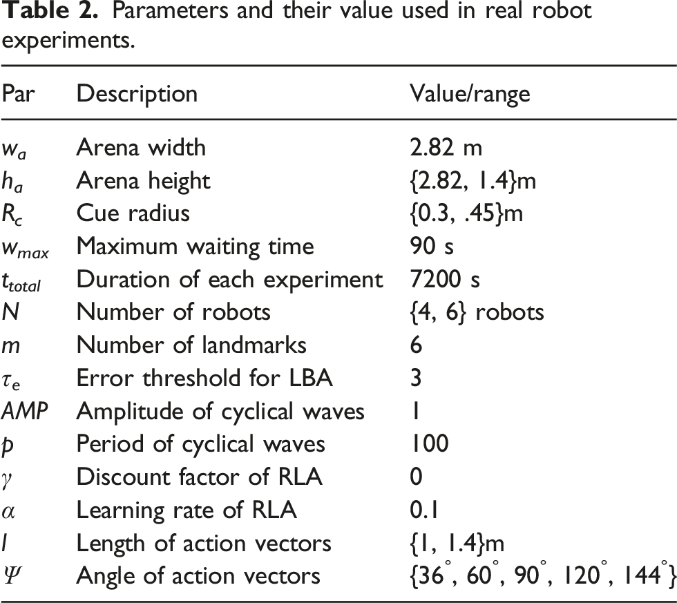
Par	Description	Value/range
w _a	Arena width	2.82 m
h _a	Arena height	{2.82, 1.4}m
R _c	Cue radius	{0.3, .45}m
w _max	Maximum waiting time	90 s
t _total	Duration of each experiment	7200 s
N	Number of robots	{4, 6} robots
m	Number of landmarks	6
τ _e	Error threshold for LBA	3
AMP	Amplitude of cyclical waves	1
p	Period of cyclical waves	100
γ	Discount factor of RLA	0
α	Learning rate of RLA	0.1
l	Length of action vectors	{1, 1.4}m
Ψ	Angle of action vectors	{36^°, 60^°, 90^°, 120^°, 144^°}

Three aggregation methods were implemented on the real robots: BEECLUST, LBA, and RLA, with cyclical schedule for ɛ. The error threshold parameter for the LBA method was τ_e = 3, and for the RLA method, amplitude and period of cycles were chosen as AMP = 1, p = 100, respectively. For the real-robot experiments, only static environment was studied, and no noise was added during the experiment. However, noise still existed due to wheel slippage and odometry errors. Different than the kinematic simulation setup where action space $A$ consists of 44 displacement vectors, in real-robot experiments, due to time limitation, the size of the action space was reduced to 6 vectors. This reduced the learning time for the reinforcement learning algorithm considerably. The action space for the N = 4 robots setup is $l \in L = {1,1.4}$ m and ψ ∈ ⊝ = {36^°, 90^°, 144^°} and for the N = 6 robots setup is $l \in L = {1,1.4}$ m and ψ ∈ ⊝ = {60^°, 90^°, 120^°}. Action space was chosen in a way that displacement vectors could span the arena properly.

A new set of kinematic-based simulations were performed with the same settings as the real-robot experiments for comparison. The only difference was that noise of σ_n = 30^° was added in kinematic-based simulations to match the inherent noise in real robots. Results were reported as steady-state values of NAS. Each experiment was repeated five times to make sure that the results were less dependent on the initial conditions. Thus, the experiments produced total 60 hours of data used for further analysis of the proposed method performance. Such a duration is comparable to experiments in works that explicitly address long-term performance of robotic swarms.

5. Results and discussion

5.1. Kinematic-based simulator experiments

5.1.1. Environment experiments

Time evolution of the NAS values for the three methods with and without odometry noise is plotted in Figure 7. In the experiments without noise, as shown in Figure 7(a), all the methods, except the BEECLUST method, showed a similar steady-state performance during the first half of the experiment reaching a NAS value of .7. When the cue location was changed, the LBA method adapted to the change faster than the RLA method. The BEECLUST method performed worst with a NAS value of .37 since the low-robot density decreased the probability of robot-robot encounters. On the other hand, its performance was not affected by the change of cue. The reason is the random nature of the BEECLUST method; since it does not exploit any information for finding the location of the cue, altering the cue location does not affect the BEECLUST method.

Figure 7.

Environment Experiments. Time evolution of the NAS values of the BEECLUST method, the LBA method with τ_e = 4, the RLA method with the cyclical schedule, p = 100, and with the VDBE schedule, σ = 1 are shown. (a) The NAS values without odometry noise and (b) the NAS values with odometry noise, σ_n = 15^°. Shades represent the first and third quartiles, and the solid lines are the median of 5 trials. Duration of each experiment is t_total = 100,000 s. The location of the cue is changed at t_change = 50,000 s, indicated by the vertical dashed line. In order to smoothen the results, moving average with a window of [t_s, t_s + 500] is used.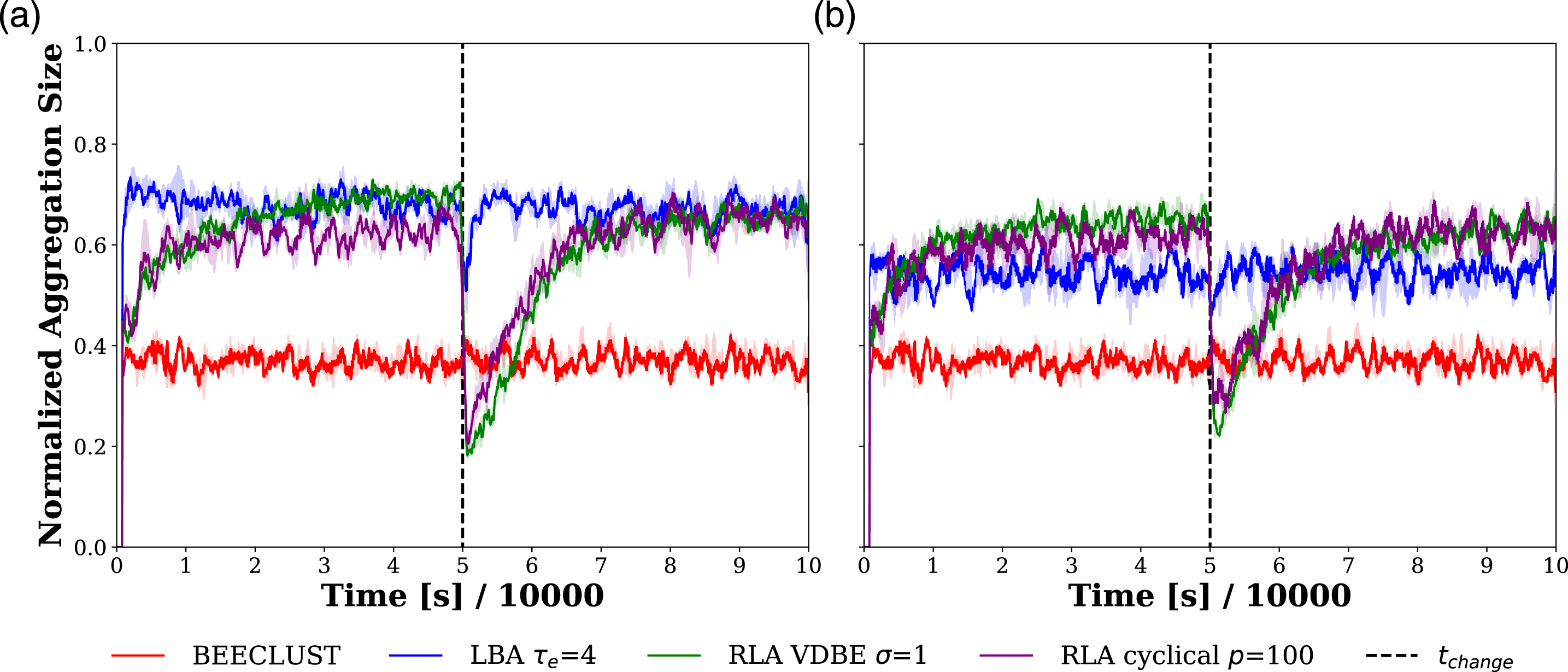

The RLA method with VDBE and cyclical schedule was able to reach the performance of the LBA method. The response of the RLA method is slower than the LBA method, and it also adapts slower to the change of cue position. This is because it takes time for the robots to explore and learn the environment to form the Q-table. In addition, the learning speed is controlled by the learning rate, α, and it is taken as a fixed value, α = .1 in this article.

To further show whether the RLA method allows robots to learn appropriate actions using maximum Q-values, the actions with maximum Q-values for each landmark observation are investigated with an experiment. In the experiment, the robots learn the Q-table implementing the RLA method under the setting of zero noise strength, σ_n = 0 and with cyclical ɛ schedule with period p = 100 and amplitude AMP = 1. The Q-tables of all robots were averaged at steady-state and for each landmark, action with maximum Q-value was shown as a red vector in Figure 8. The results indicate that the learned actions with the RLA method lead the robots towards the cue region with a higher cue intensity compared to other actions.

Figure 8.

Representation of the learned actions that yield the maximum Q-value (shown as red vectors) for each state, compared to the other actions (shown as pink vectors) in steady-state.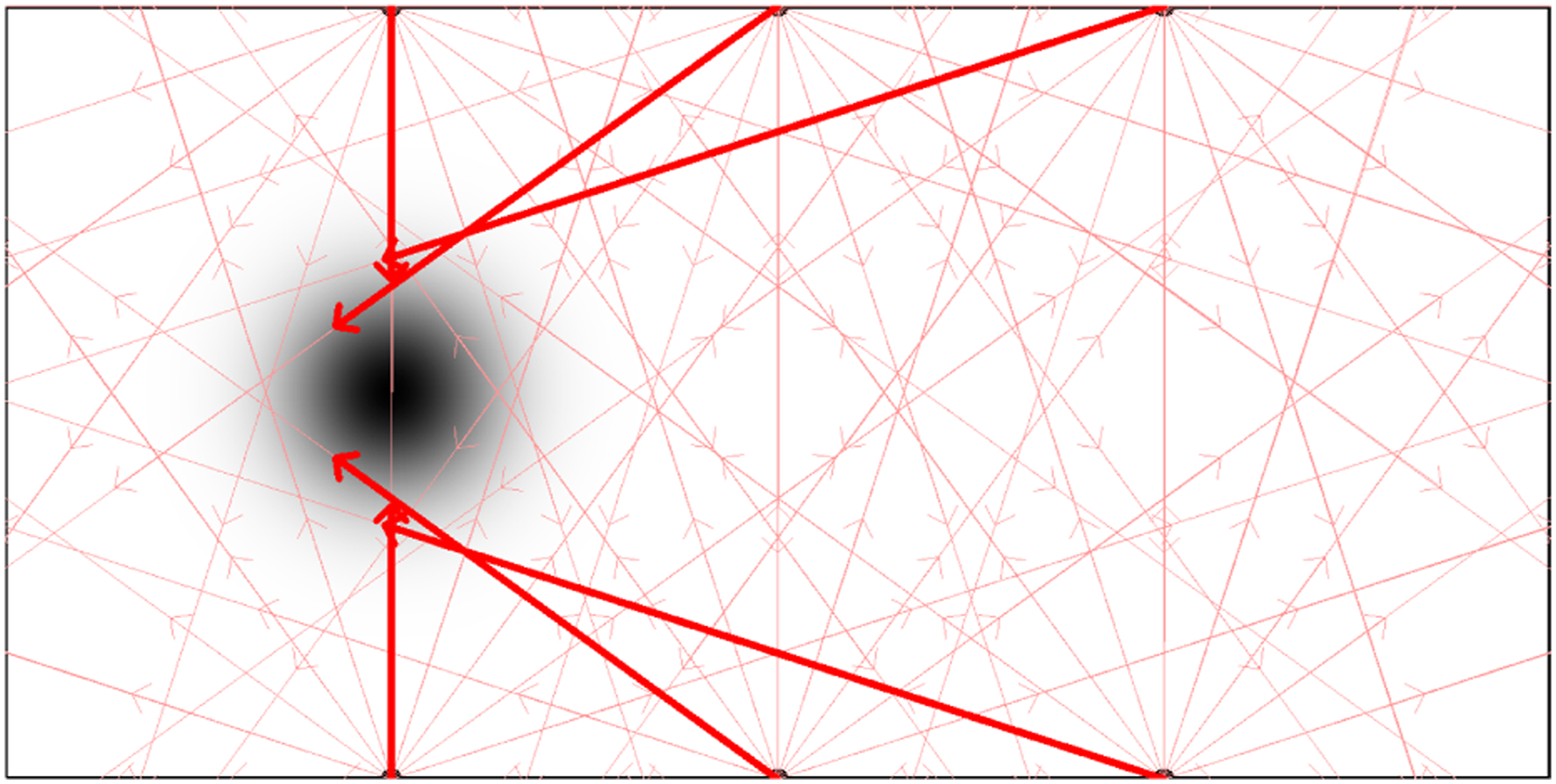

The results of the experiments with odometry noise, σ_n = 15^°, are shown in Figure 7(b). When compared to the experiments without noise, the performance of all methods except the BEECLUST method decreased. The LBA method has the most drastic decrease from a NAS value of .7 to .55, whereas the RLA method showed a slight decrease from .7 to .67. The reason is the performance of the LBA method depends heavily on the odometry data. Therefore, a slight amount of noise like σ_n = 15^° affects the LBA method considerably. On the other hand, the RLA method also uses the odometry data to execute an action, but it does not integrate displacement vectors. Therefore, it is more robust to odometry noise.

5.1.2. Noise experiments

The results of the noise experiments are shown in Figure 9. In the zero noise case, the LBA method performed best with a NAS value of approximately .7. However, its performance decreased dramatically as noise increased since the LBA method depends heavily on the odometer readings. The performance of the RLA method also decreased due to noise, especially in higher noise regions, but still, it is more robust to noise than the LBA method. Since the BEECLUST method does not use the odometry readings, its performance did not change and stayed around .37 in all the settings. When σ_n = 180^°, the performance of all methods converged to BEECLUST because the information acquired from landmark is not exploitable anymore due to the intense amount of noise.

Figure 9.

Noise Experiments. The steady-state values of NAS are shown for the BEECLUST, LBA, RLA with cyclical schedule, and RLA with VDBE schedule methods with respect to the odometry noise, σ_n ∈ {0^°, 5^°, 15^°, 30^°, 45^°, 60^°, 90^°, 135^°, 180^°}. Bars represent the first and third quartiles, and lines are the median of 5 trails. The experiments are static and duration of each experiment is: t_total = 50,000 s. The x-axis is not drawn to scale.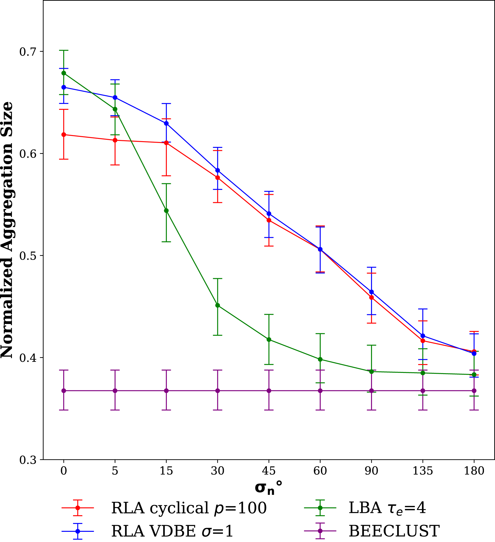

5.1.3. Parameter sensitivity experiments

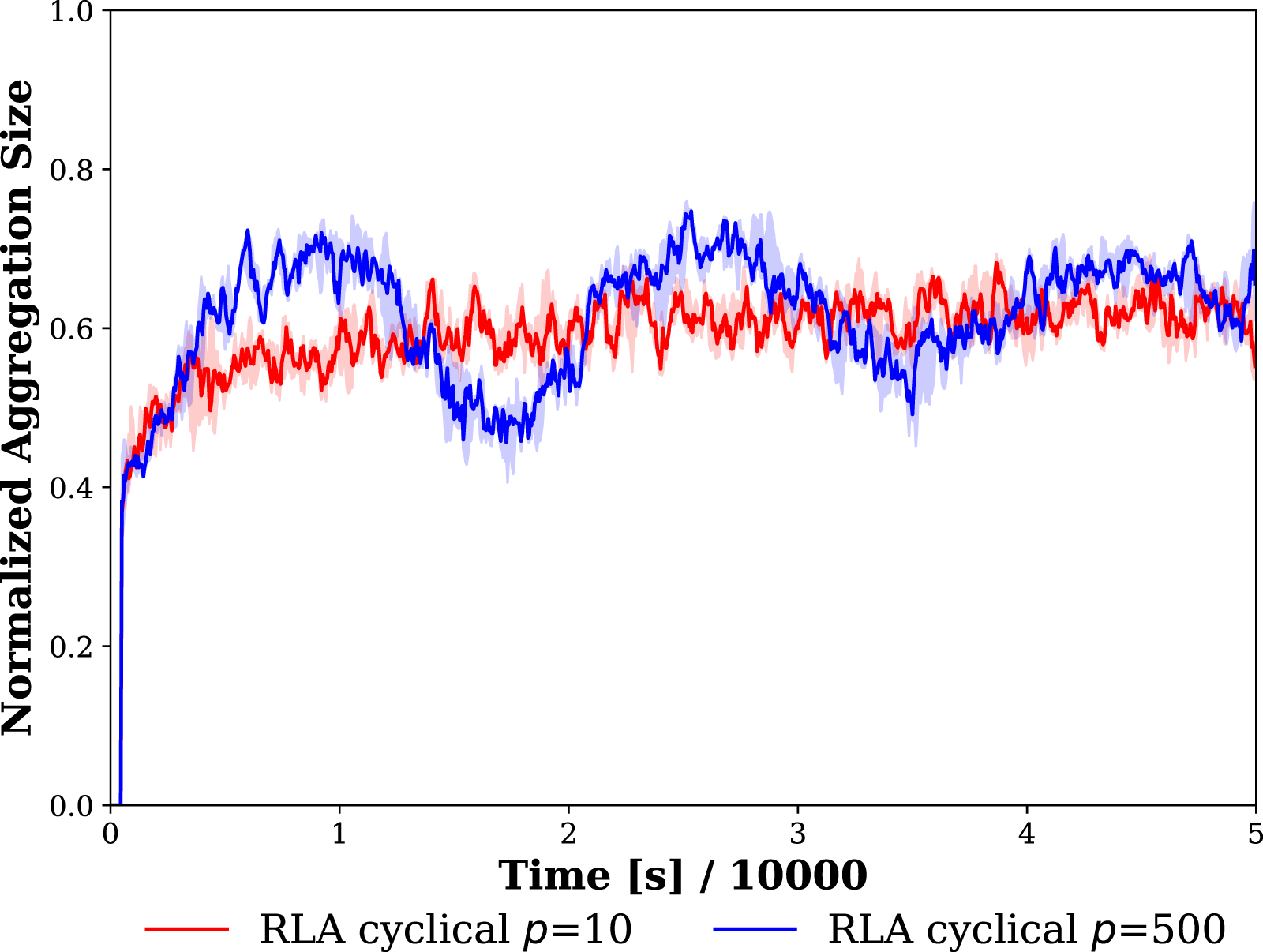
The experimental results investigating the sensitivity of the cyclical and VDBE ɛ schedules with respect to their parameters revealed that the cyclical schedule is less affected by changes in its period and amplitude of ɛ oscillations compared to variations in the σ parameter of the VDBE schedule. The results show that the cyclical scheduling is more effective in the dynamic environments, and the VDBE scheduling is more beneficial with its fine-tuned parameter in the static environments.

The steady-state values of NAS versus the model parameters are shown in Figure 10. The first and second rows plot the steady-state values before and after the change of location of the cue. The leftmost and middle columns are the plots of the period, p, and amplitude, AMP, parameters of the cyclic schedule, and the last column are the plots of the inverse sensitivity parameter, σ for the VDBE schedule. In case of cyclical schedule, the period did not affect the aggregation performance when p ≤ 10. When p ≥ 10, the performance increased considerably and remained around a NAS value of .65, indicating that NAS performance does not change considerably when p ≥ 10. Although large periods did not affect the steady-state value of the performance, they cause oscillations of NAS values as shown in Figure 11. In case of the amplitude parameter, it did not affect the performance for AMP ≥.37, and the NAS value remained around .6. For both cyclical schedule parameters, p and AMP, the results were the same before and after the change of the cue, meaning that the cyclical schedule is adaptive to environmental changes.

Figure 10.

Parameter Sensitivity Experiments. The steady-state values of NAS are shown for different model parameters of RLA method with cyclic schedule and RLA method with VDBE schedule. Top and bottom rows show the results before and after the change of cue location, respectively. Leftmost and middle columns show the results for the period, p (AMP is taken as 1), and amplitude, AMP (p is taken as 100) parameters of the cyclic schedule, respectively. The rightmost column shows the results for the inverse sensitivity (σ) parameter of the VDBE schedule. Bars represent the first and third quartiles, and lines are the median of 5 trails. Duration of each experiment is t_total = 100,000 s. The location of the cue is changed at t_change = 50,000 s. The leftmost and rightmost plots are drawn in semi-log scale.

Figure 11.

Demonstration of effect of period parameter, p, of cyclical schedule of the RLA method on performance of the swarm. Shades demonstrate the first and third quartiles, and lines are the mean of 5 trials of the experiment.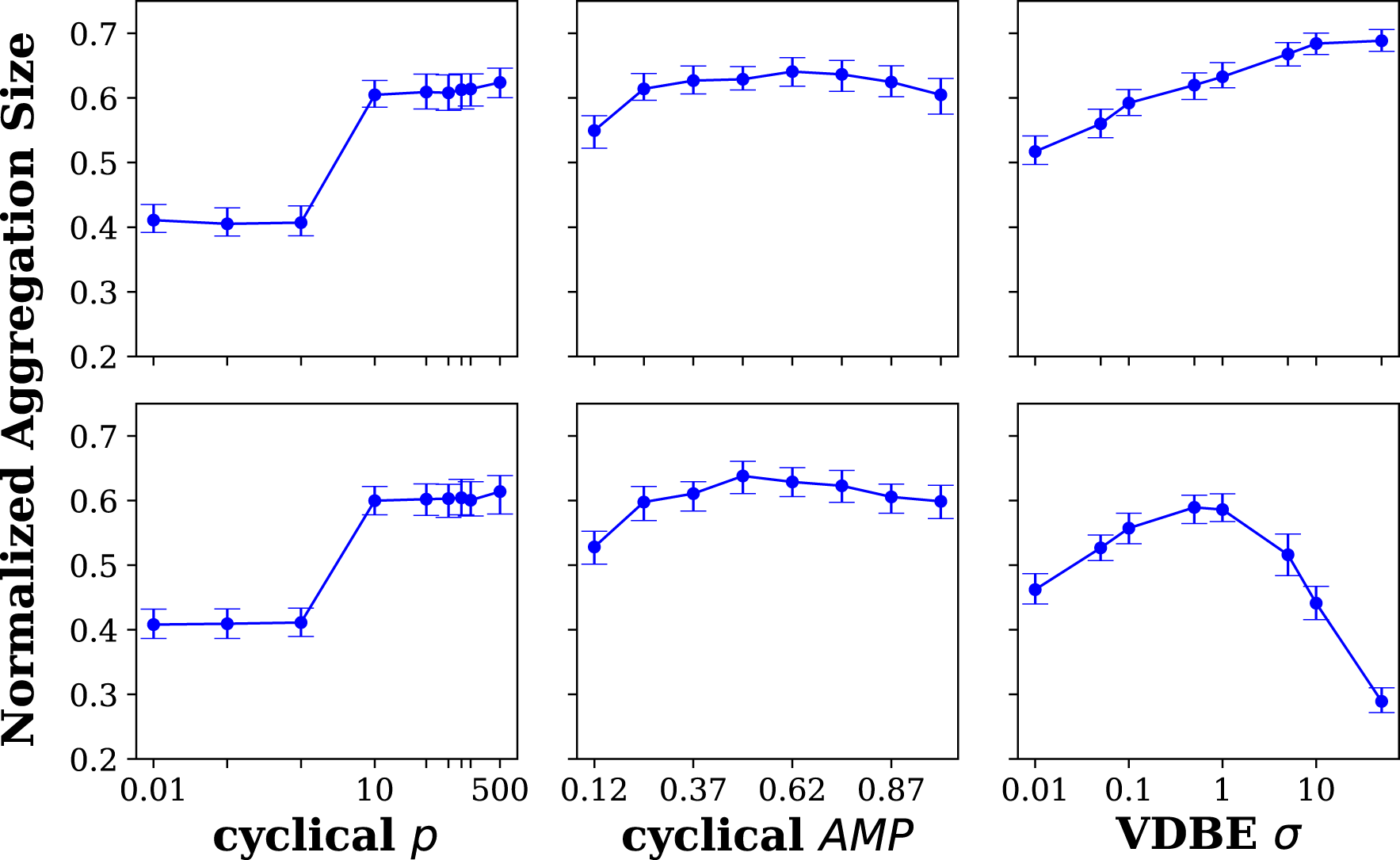

However, in case of the VDBE schedule, σ drastically changes the performance of aggregation. Before the change of the location of the cue, higher σ values yielded better results, indicating better performance of VDBE schedule in static environments. However, after the location of the cue was changed, higher σ values failed to put robots back to the exploration state, decreasing the aggregation performance. For instance, when σ = 50, the NAS value before the change of the cue was approximately .7, and after the change, it dropped to .3, which is even worse than the performance of the BEECLUST method (NAS = .37). This is because robots do not return to the exploration mode; hence, they use the previously learned Q-table in the new environment, and performance becomes worse than the random choice.

In order to understand the performance difference between the two schedules, the time evolution of ɛ for the cyclical schedule with p = 100 and AMP = 1 and the VDBE schedule with σ = 50 using the data from a randomly selected robot is depicted in Figure 12. For the cyclical schedule, ɛ changes periodically based on p and AMP. VDBE schedule updates ɛ for each state separately, one line was drawn for each state making a total of six lines.

Figure 12.

Evolution of ɛ during time for VDBE schedule with σ = 50 and cyclical schedule with p = 100 for a randomly selected robot. Occasional straight line regions in ɛ is due to the fact that ɛ is updated at every epoch, that is, when the robot detected a landmark. So, ɛ is a function of epoch, not time.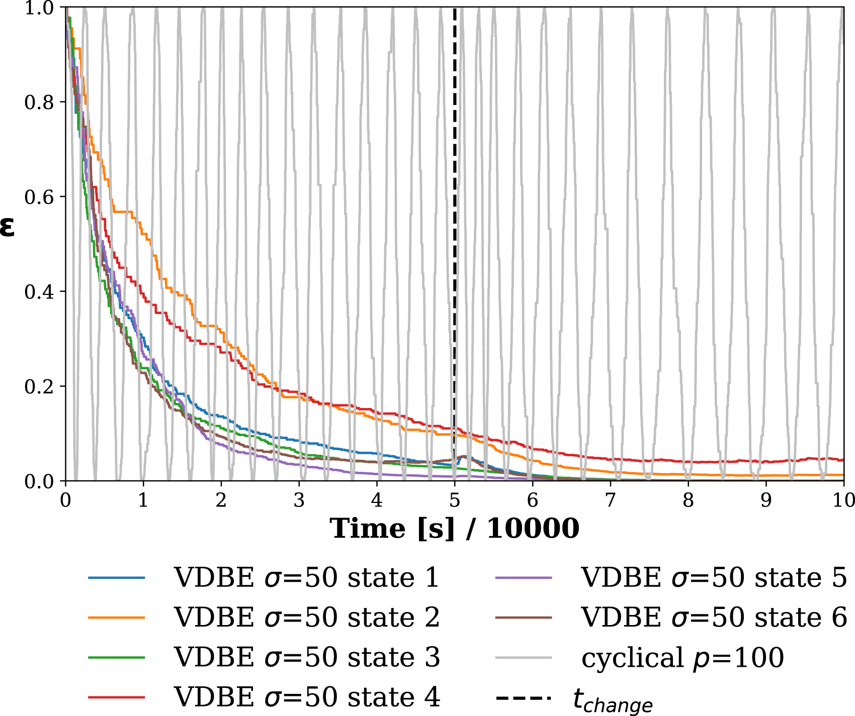

Rewards received by a randomly selected robot for the cyclical and VDBE schedules are depicted in Figure 13. Rewards that VDBE schedule receives were higher than the cyclical schedule before the change of the cue, which indicates superior performance of the VDBE schedule in static environments. However, after environment change, the VDBE schedule keeps ɛ low, as shown in Figure 12 and fails to adapt to the new location of the cue showing better adaptability of the cyclical schedule to dynamic environments.

Figure 13.

Average reward received by robots during time for RLA method with cyclical ɛ schedule with a period of p = 100 and an amplitude of AMP = 1 and VDBE schedule with σ = 50. Shades represent the first and third quartiles, and lines are the median of 5 trails. Duration of each experiment is t_total = 100,000 s. The location of the cue is changed at t_change = 50,000 s, indicated by the vertical dashed line.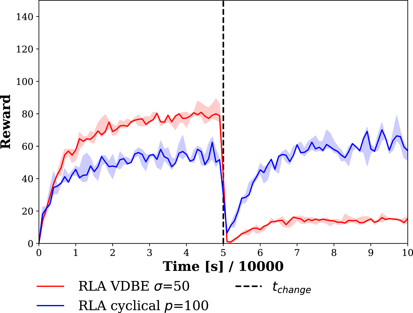

5.2. Real-robot experiments

The BEECLUST, LBA, and RLA methods were implemented using the real robots. For the sake of comparison, the same experimental setup was also implemented using the kinematic-based simulator. The steady-state NAS values for the real-robot and the simulation-based experiments with N = 4 and N = 6 robots are shown in Figure 14(a) and (b), respectively. In N = 4 robots experiment, the BEECLUST method had the lowest performance with a steady-state NAS value of .45, the LBA method had a steady-state performance of .58, and the RLA method had the best performance reaching up to .62. In N = 6 robots experiment, a similar trend in performance has been observed. The results of kinematic-based simulation experiments are in accordance with the real-robot experiments.

Figure 14.

Steady-state values of NAS performance of the BEECLUST, LBA, and RLA methods for real robots experiments with (a) N = 4 robots and (b) N = 6 robots. RLA method is implemented with cyclic schedule using AMP = 1 and p = 100. The boxes represent the median, first, and third quartiles. Whiskers are the minimum and maximum values. The pink boxes represent the results of kinematic-based simulation results, and the blue boxes are real-robot experiment results. Experiments are repeated five times.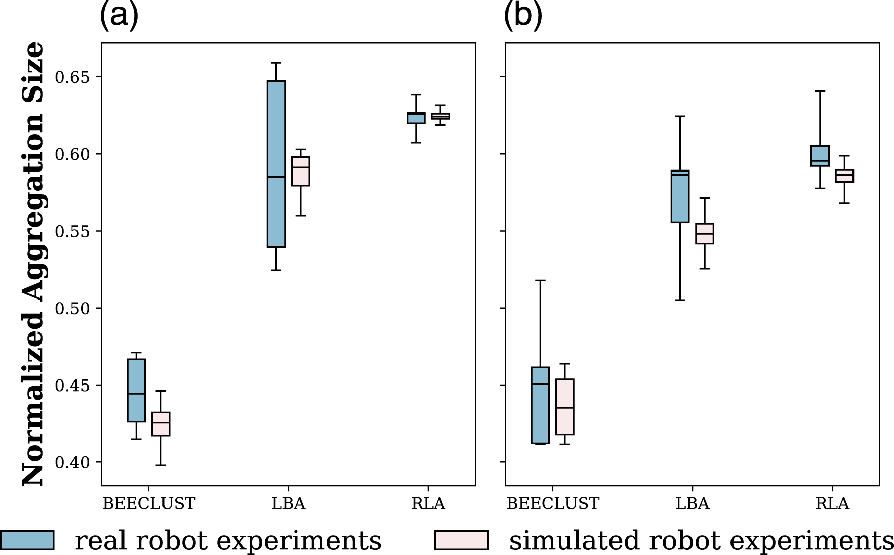

5.3. Discussion

In the environment experiments, since the robot density was low, the BEECLUST method had the worst performance, as shown in Figure 7. For the experiments without noise, the LBA method showed the best performance. However, its performance dropped drastically in the experiments with even a slight amount of noise (Figure 9). The RLA method was more robust to noise than the LBA method. This is also observed in real-robot experiments (Figure 14) where odometry noise was inherently present. From the performance perspective, these results imply that the RLA method managed to aggregate most of the robots on the cue despite the presence of inaccuracy and drift in odometry. This result proves the robustness of RLA method to sensory noise and its applicability in real-world scenarios.

The RLA method uses the Q-learning technique, and ɛ-greedy policy was chosen as the policy to tackle the exploration-exploitation dilemma. In order to use the ɛ-greedy policy effectively in noisy and dynamic environments, ɛ must be scheduled. VDBE (Tokic, 2010) scheduling schemes were implemented, and a new cyclical schedule was proposed using the results in Smith (2017). The RLA method with VDBE schedule achieved the highest performance with proper tuning of the model parameters (Figure 9). However, its performance is very sensitive to model parameters (Figure 10). On the other hand, the RLA method with cyclical schedule is more robust to odometry noise (Figure 9), less sensitive to model parameters (Figure 10), and performs better in non-stationary environments (Figure 7). Furthermore, the cyclical schedule requires less computational power and memory, suitable for simple swarm robots (Figure 14). The result on the cyclical schedule showed that it improves the performance of the RLA method and makes it more applicable in real-world scenarios.

Swarm robotic systems can be used for the tasks dealing with hazardous substances or items that could be dangerous for humans and that are challenging for a single robot (Huang et al., 2019). For example, a swarm robotic system using the RLA method can be used to decontaminate chemical leakage in a damaged factory, where human operators or a single robot are not sufficient to deal with this task. Furthermore, the RLA method is likely to be robust on any sensory noises inside the damaged factory, such as the low quality camera input due to poor light condition and high degree of odometry error due to harsh conditions inside the factory. The advantage of the RLA method in real-world applications is further supported by the research on swarm robotic aggregation for pipeline inspection on water, oil, waste, and chemical reactor vessels. In Duisterwinkel et al. (2018); Andraud et al. (2018), the results suggest that the aggregation of robot swarms for inspection in harsh environments must be robust against sensor noise. The effect of environmental conditions on the robot swarm aggregation is also reported in Na et al. (2021). Therefore, RLA method can provide viable solution for robot swarm aggregation tasks in such hazardous environments under high sensory environmental noise.

In the VDBE schedule, the inverse sensitivity parameter, σ, needs fine-tuning, which is one of the disadvantages of VDBE. The other disadvantage of VDBE is that each state requires its own independent ɛ, which makes ɛ a function of the state, s. Consequently, as the number of states grows, the VDBE schedule will require more memory to store ɛ parameters for each state. For environments with a large state space size, the VDBE schedule consumes a considerable amount of memory to keep track of each ɛ independently.

It should also be noted that the learning rate was set to a fixed value α = .1. Although a constant choice of α will restrict the convergence speed of the model and prevent it from reaching its best performance, studying adaptive and more advanced schedules for α is beyond the scope of this article, and it is considered a future work.

Moreover, the length of action vectors in the RLA method, l, depends on the arena size. More vectors will span the arena better, and chances of finding actions with higher rewards will increase. However, since increasing the size of the action space will increase the Q-table size, training time will grow. On the other hand, a smaller action space size will cause faster learning, but the arena will not be spanned properly. Choosing the size of the action space as 44 is a fair trade-off between not having a large Q-table and spanning the arena sufficiently. In reality, the aggregation problem has continuous action space, but solving the aggregation problem in continuous space is beyond the scope of this article.

It should be noted that since landmarks represent the states of the Q-learning algorithm, increasing the number of landmarks will increase the size of the Q-table hence increasing the training time. On the other hand, choosing fewer landmarks will reduce the probability of their detection and hinder the performance of the LBA and RLA methods. By selecting the number of landmarks as m = 6 for our test cases, the Q-table does not become too large, and still, the performance of the LBA and RLA methods are at acceptable levels.

To address the similarity of the RLA method to Simultaneous Localization And Mapping methods (SLAM), it is worth bearing in mind that the distribution of the landmarks in the arena is sparse, causing the robots to detect them only occasionally and detecting only one landmark at a time. This is analogous to low visibility situations (e.g., in disaster scenarios, adverse weather, or crowded locations), where SLAM struggle (Cadena et al., 2016; Gomez-Ojeda et al., 2020; Li et al., 2020).

6. Conclusion

In this article, a novel cue-based aggregation method was proposed (RLA) based on Q-learning and ɛ-greedy policy. Through systematic analysis with the kinematic-based simulations and real robots experiments, it was shown that the proposed method shows better performance in the presence of odometry noise and environment uncertainties when compared to the BEECLUST method (Schmickl & Hamann, 2011) and the LBA method (Sadeghi Amjadi et al., 2021); and it is applicable in real robots. A new approach to solve the exploration-exploitation dilemma was proposed to schedule ɛ parameter of ɛ-greedy policy. The proposed cyclical schedule was compared to the other state-of-the-art approaches, and it was shown that cyclical updates are less sensitive to model parameters and do not require fine-tuning. Additionally, cyclical updates of ɛ make robots more robust to changes in the environment.

Nevertheless, the proposed aggregation method requires a priori information about the dimensions of the arena. Therefore, as future work, the Deep Deterministic Policy Gradient algorithm (Lillicrap et al., 2015) will be used to avoid requiring a priori information about dimensions of the arena. Furthermore, an adaptive approach will be considered to tune the learning speed of the algorithm.

We plan to deploy the proposed approach in scenarios of robot-insect interaction, where groups of robots aggregate around key agents of social insect colonies to affect their behavior and overall colony activity (Stefanec et al., 2022).

Footnotes

Acknowledgements

The presented work was supported by EU-H2020-FET RoboRoyale project, grant agreement No. 964492 and by the Czech Ministry of Education by OP VVV funded project CZ.02.1.01/0.0/0.0/16 019/0000765 “Research Center for Informatics”.

Declaration of conflicting interests

The author(s) declared no potential conflicts of interest with respect to the research, authorship, and/or publication of this article.

Funding

The author(s) disclosed receipt of the following financial support for the research, authorship, and/or publication of this article: This work was supported by the EU-H2020-FET RoboRoyale project (964492).

ORCID iD

Farshad Arvin

About the Authors

Arash Sadeghi Amjadi is a PhD student in computer science at Memorial University of Newfoundland. He completed his Master’s degree in mechanical engineering at Middle East Technical University under the supervision of Dr Ali Emre Turgut in 2021. He holds a Bachelor’s degree in Electrical Engineering from Tabriz University earned in 2019. His research focuses on swarm robotics, deep learning, machine learning, control and systems engineering, and autonomous robotic systems.

Cem Bilaloğlu received BSc and MSc degrees in mechanical engineering from the Middle East Technical University, Turkey. During his master’s studies, he developed Kobot swarm robot platform at the Kovan Research Laboratory. Currently, he is a PhD student at École Polytechnique Fédérale de Lausanne and a research assistant at Idiap research institute in Switzerland. His research interests include machine learning, optimal control, and swarm robotics.

Ali Emre Turgut has received a BSc in mechanical engineering from Middle East Technical University, Turkey, in 1996; an MSc in mechanical engineering from Middle East Technical University, Turkey, in 2000; and PhD in mechanical engineering from Middle East Technical University at Kovan Research Laboratory, Turkey, in 2008. He worked as a post-doctoral researcher at Universite Libre de Bruxelles, IRIDIA, Belgium, and as a research associate at the department of biology at KU Leuven, Belgium during 2008–2012. In 2013, he worked as an assistant professor in the Department of Mechatronics Engineering at the University of Aeronautical Association of Turkey. He worked as a research associate in the Laboratory of Socioecology and Social Evolution, KU Leuven. He started working in the mechanical engineering department at Middle East Technical University as an assistant professor in 2015.

Seongin Na is a PhD candidate in robotics at the Swarm & Computational Intelligence Laboratory (SwaCIL) at the University of Manchester. He was awarded a President’s Doctoral Scholar Award for his PhD study from the University of Manchester. Prior to his PhD study, he received a B.Eng in Mechatronic Engineering from the University of Manchester, United Kingdom in June 2019. His research interest is swarm robotics, deep reinforcement learning, and federated learning.

Erol Şahin is the founding director of METU-ROMER (Center for Robotics and AI) and the KOVAN research lab. He has a PhD in Cognitive and Neural Systems from Boston University, B.S. and M.S. in Electrical and Electronics Engineering from Bilkent University, and Computer Engineering from METU. Dr Sahin worked as a post-doctoral researcher at IRIDIA of Universite Libre de Bruxelles, before assuming his faculty position at the Dept. of Computer Engineering of METU. Dr Sahin’s research has focused on swarm robotics, robotic learning, and human-robot interaction during the last decade receiving more than 2,000,000*** of funding from the EU, TUBITAK, and industry. In particular, he has received funding from the Turkish Government to build a center for robotics and AI research at METU. Besides publishing in major conferences and journals, Dr Sahin has edited three journal special issues, three conference proceedings, and two books. In 2007, he was awarded an iCub humanoid platform from the RobotCub consortium for his research in robotic learning. Between 2013 and 2015, Dr Sahin visited the Robotics Institute of Carnegie Mellon University, USA, through a Marie Curie Fellowship. Dr Sahin has been an Associate Editor for the Adaptive Behavior journal and an Editorial Board member of the Swarm Intelligence journal.

Tomáš Krajník is an associate professor at the Czech Technical University in Prague and a founding director of the Chronorobotics laboratory, which aims at the problems related to perception and spatio-temporal representations for long-term autonomy of mobile robots in changing environments. His team designed and implemented a robust and efficient system for real-time and long-term localization of robot swarms. Tomáš Krajník participated in several EU and international projects and before returning to Czechia, he was part of the Lincoln Centre for Autonomous Systems Research, led by Prof. Tom Duckett.

Farshad Arvin received the BSc degree in Computer Engineering, the MSc degree in Computer Systems engineering, and the PhD degree in Computer Science, in 2004, 2010, and 2015, respectively. Farshad is an Associate Professor in Robotics in the Department of Computer Science at Durham University in UK. Prior to that, he was a Senior Lecturer in Robotics at The University of Manchester, UK. He visited several leading institutes including Artificial Life Laboratory with the University of Graz, Institute of Microelectronics, Tsinghua University, Beijing, and Italian Institute of Technology (iit) in Genoa as a Senior Visiting Research Scholar. His research interests include swarm robotics and autonomous multi-agent systems. He is the founding director of the Swarm & Computation Intelligence Laboratory (SwaCIL) formed in 2018.

References

Andraud

Hallawa

De Roose

Cantatore

Ascheid

Verhelst

(2018). Evolving hardware instinctive behaviors in resource-scarce agent swarms exploring hard-to-reach environments. In Proceedings of the genetic and evolutionary computation conference companion (pp. 1497–1504). Association for Computing Machinery.

Arvin

Turgut

A. E.

Krajník

Yue

(2016). Investigation of cue-based aggregation in static and dynamic environments with a mobile robot swarm. Adaptive Behavior, 24(2), 102–118. https://doi.org/10.1177/1059712316632851

Baggio

D. L.

Emami

Escriva

D. M.

Ievgen

Mahmood

Saragih

Shilkrot

(2012). Mastering OpenCV with practical computer vision projects. Packt Publishing.

Barmak

Stefanec

Hofstadler

D. N.

Piotet

Schönwetter-Fuchs-Schistek

Mondada

Schmickl

Mills

(2023). A robotic honeycomb for interaction with a honeybee colony. Science Robotics, 8(76), Article eadd7385.

Cadena

Carlone

Carrillo

Latif

Scaramuzza

Neira

Reid

Leonard

J. J.

(2016). Past, present, and future of simultaneous localization and mapping: Toward the robust-perception age. IEEE Transactions on Robotics, 32(6), 1309–1332. https://doi.org/10.1109/TRO.2016.2624754

Camazine

Deneubourg

Franks

Sneyd

Bonabeau

Theraula

(2003). Self-organization in Biological systems. Princeton studies in complexity. Princeton University Press.

Collett

T. S.

(1996). Insect navigation en route to the goal: Multiple strategies for the use of landmarks. Journal of Experimental Biology, 199(1), 227–235. https://doi.org/10.1242/jeb.199.1.227

Douglas

D. H.

Peucker

T. K.

(1973). Algorithms for the reduction of the number of points required to represent a digitized line or its caricature. Cartographica: The International Journal for Geographic Information and Geovisualization, 10(2), 112–122. https://doi.org/10.3138/FM57-6770-U75U-7727

Doya

Samejima

Katagiri

Kawato

(2002). Multiple model-based reinforcement learning. Neural Computation, 14(6), 1347–1369. https://doi.org/10.1162/089976602753712972

10.

Duisterwinkel

E. H. A.

Talnishnikh

Krijnders

Wortche

H. J.

(2018). Sensor motes for the exploration and monitoring of operational pipelines. IEEE Transactions on Instrumentation and Measurement, 67(3), 655–666. https://doi.org/10.1109/TIM.2017.2775404

11.

Frank

D. D.

Jouandet

G. C.

Kearney

P. J.

MacPherson

L. J.

Gallio

(2015). Temperature representation in the drosophila brain. Nature, 519(7543), 358–361. https://doi.org/10.1038/nature14284

12.

Franzoni

Biondi

Milani

(2020). Exploring negative emotions to preserve social distance in a pandemic emergency. In International conference on computational science and its applications (pp. 562–573). Springer Nature.

13.

Furgale

Barfoot

T. D.

(2010). Visual teach and repeat for long-range rover autonomy. Journal of Field Robotics, 27(5), 534–560. https://doi.org/10.1002/rob.20342

14.

Garnier

Jost

Gautrais

Asadpour

Caprari

Jeanson

Grimal

Theraulaz

(2008). The embodiment of cockroach aggregation behavior in a group of micro-robots. Artificial Life, 14(4), 387–408. https://doi.org/10.1162/artl.2008.14.4.14400

15.

Garrido-Jurado

Muñoz-Salinas

Madrid-Cuevas

F. J.

Marín-Jiménez

M. J.

(2014). Automatic generation and detection of highly reliable fiducial markers under occlusion. Pattern Recognition, 47(6), 2280–2292. https://doi.org/10.1016/j.patcog.2014.01.005

16.

Gomez-Ojeda

(2020). Robust visual slam in challenging environments with low-texture and dynamic illumination. Dialnet.

17.

Goodenough

A. E.

Little

Carpenter

W. S.

Hart

A. G.

(2017). Birds of a feather flock together: Insights into starling murmuration behaviour revealed using citizen science. PLoS One, 12(6), Article e0179277.

18.

Grünbaum

Okubo

(1994). Modelling social animal aggregations. In Frontiers in mathematical biology (pp. 296–325). Springer.

19.

Gutiérrez

Campo

Monasterio-Huelin

Magdalena

Dorigo

(2010). Collective decision-making based on social odometry. Neural Computing & Applications, 19(6), 807–823. https://doi.org/10.1007/s00521-010-0380-x

20.

Halloy

Sempo

Caprari

Rivault

Asadpour

Tâche

Saïd

Durier

Canonge

Amé

J. M.

Detrain

Correll

Martinoli

Mondada

Siegwart

Deneubourg

J. L.

(2007). Social integration of robots into groups of cockroaches to control self-organized choices. Science, 318(5853), 1155–1158. https://doi.org/10.1126/science.114425

21.

Halodová

Dvořráková

Majer

Vintr

Mozos

O. M.

Dayoub

Krajník

(2019). Predictive and adaptive maps for long-term visual navigation in changing environments. In 2019 IEEE/RSJ International Conference on Intelligent Robots and Systems (IROS) (pp. 7033–7039). IEEE.

22.

Heran

(1952). Untersuchungen über den temperatursinn der honigbiene (apis mellifica) unter besonderer berücksichtigung der wahrnehmung strahlender wärme. Zeitschrift für Vergleichende Politikwissenschaft, 34(2), 179–206. https://doi.org/10.1007/BF00339537

23.

Huang

Arvin

West

Watson

Lennox

(2019). Exploration in extreme environments with swarm robotic system. In 2019 IEEE International Conference on Mechatronics (ICM) (vol. 1, pp. 193–198). IEEE.

24.

Hüttenrauch

Adrian

Neumann

, et al. (2019). Deep reinforcement learning for swarm systems. Journal of Machine Learning Research, 20(54), 1–31.

25.

Krajník

Faigl

Vonásek

Košnar

Kulich

Přeučil

(2010). Simple yet stable bearing-only navigation. Journal of Field Robotics, 27(5), 511–533. https://doi.org/10.1002/rob.20354

26.

Krause

Ruxton

G. D.

Ruxton

I. G.

(2002). Living in groups. Oxford University Press.

27.

Kumar

S. A.

Sharma

Vanualailai

Prasad

(2021). Stable switched controllers for a swarm of ugvs for hierarchal landmark navigation. Swarm and Evolutionary Computation, 65, 100926. https://doi.org/10.1016/j.swevo.2021.100926

28.

Lemmens

Tuyls

(2009). Stigmergic landmark foraging. Proceedings of The 8th International Conference on Autonomous Agents and Multiagent Systems, 1, 497–504.

29.

Brasch

Wang

Navab

Tombari

(2020). Structure-slam: Low-drift monocular slam in indoor environments. IEEE Robotics and Automation Letters, 5(4), 6583–6590. https://doi.org/10.1109/LRA.2020.3015456

30.

Lillicrap

T. P.

Hunt

J. J.

Pritzel

Heess

Erez

Tassa

Silver

Wierstra

(2015). Continuous control with deep reinforcement learning. arXiv preprint arXiv:1509.02971.

31.

Misir

Gökrem

(2021). Dynamic interactive self organizing aggregation method in swarm robots. Biosystems, 207, 104451. https://doi.org/10.1016/j.biosystems.2021.104451

32.

Niu

Lennox

Arvin

(2022). Bio-inspired collision avoidance in swarm systems via deep reinforcement learning. IEEE Transactions on Vehicular Technology, 71(3), 2511–2526. https://doi.org/10.1109/TVT.2022.3145346

33.

Qiu

Turgut

A. E.

Ulrich

Krajník

Yue

Lennox

Arvin

(2021). Bio-inspired artificial pheromone system for swarm robotics applications. Adaptive Behavior, 29(4), 395–415. https://doi.org/10.1177/1059712320918936

34.

Paton

MacTavish

Berczi

L.-P.

van Es

S. K.

Barfoot

T. D.

(2018). I can see for miles and miles: An extended field test of visual teach and repeat 2.0. In Field and service robotics (pp. 415–431). Springer.

35.

Pham

H. X.

H. M.

Feil-Seifer

Van Nguyen

(2018). Reinforcement learning for autonomous uav navigation using function approximation. In 2018 IEEE international symposium on safety, security, and rescue robotics (SSRR) (pp. 1–6). IEEE.

36.

Quigley

Conley

Gerkey

Faust

Foote

Leibs

Wheeler

A. Y.

(2009). Ros: An open-source robot operating system. In ICRA workshop on open source software (vol. 3, p. 5). Kobe.

37.

Rahimi

Gibb

Shen

H. M.

(2018). A comparison of various approaches to reinforcement learning algorithms for multi-robot box pushing. In International conference on engineering research and applications (pp. 16–30). Springer.

38.

Rappel

W.-J.

Nicol

Sarkissian

Levine

Loomis

W. F.

(1999). Self-organized vortex state in two-dimensional dictyostelium dynamics. Physical Review Letters, 83(6), 1247. https://doi.org/10.1103/PhysRevLett.83.1247

39.

Reinhard

Srinivasan

M. V.

Guez

Zhang

S. W.

(2004a). Floral scents induce recall of navigational and visual memories in honeybees. Journal of Experimental Biology, 207(25), 4371–4381. https://doi.org/10.1242/jeb.01306

40.

Reinhard

Srinivasan

M. V.

Zhang

(2004b). Scent-triggered navigation in honeybees. Nature, 427(6973), 411. https://doi.org/10.1038/427411a

41.

Rekabi-Bana

Stefanec

Ulrich

Keyvan

E. E.

Rouček

Broughton

Y. G. B.

Şahin

Ö.

Turgut

A. E.

Şahin

Krajník

Schmickl

Arvin

(2023). Mechatronic design for multi robots-insect swarms interactions. In IEEE international conference on Mechatronics - ICM. IEEE.

42.

Sadeghi Amjadi

Raoufi

Turgut

A. E.

(2021). A self-adaptive landmark-based aggregation method for robot swarms. Adaptive Behavior, 30(1), 1059712320985543. https://doi.org/10.1177/1059712320985543

43.

Sadeghi Amjadi

Raoufi

Turgut

A. E.

Broughton

Krajník

Arvin

(2020). Cooperative pollution source exploration and cleanup with a bio-inspired swarm robot aggregation. In International conference on collaborative computing: Networking, applications and worksharing (pp. 469–481). Springer.

44.

Saleh Teymouri

Bhattacharya

(2021). Landmark-based distributed topological mapping and navigation in gps-denied urban environments using teams of low-cost robots. arXiv e-prints. arXiv–2103.

45.

Schmickl

Hamann

(2011). Beeclust: A swarm algorithm derived from honeybees. In Bio-Inspired computing and communication networks. CRC Press (March 2011).

46.

Sion

Reina

Birattari

Tuci

(2022). Controlling robot swarm aggregation through a minority of informed robots. In Swarm Intelligence: 13th International Conference, ANTS 2022, Málaga, Spain, November 2–4, 2022, Proceedings (pp. 91–103). Springer.

47.

Smith

L. N.

(2017). Cyclical learning rates for training neural networks. In 2017 IEEE winter conference on applications of computer vision (WACV) (pp. 464–472). IEEE.

48.

Srinivasan

M. V.

(2010). Honey bees as a model for vision, perception, and cognition. Annual Review of Entomology, 55(1), 267–284. https://doi.org/10.1146/annurev.ento.010908.164537

49.

Stefanec

Hofstadler

D. N.

Krajník

Turgut

A. E.

Alemdar

Lennox

Şahin

Arvin

Schmickl

(2022). A Minimally Invasive Approach Towards “Ecosystem Hacking” With Honeybees. Frontiers in Robotics and AI, 9, 791921. https://doi.org/10.3389/frobt.2022.791921

50.

Sutton

R. S.

Barto

A. G.

(2018). Reinforcement learning: An introduction. MIT press.

51.

Suzuki

(1985). Topological structural analysis of digitized binary images by border following. Computer Vision, Graphics, and Image Processing, 30(1), 32–46. https://doi.org/10.1016/0734-189X(85)90016-7

52.

Tang

Cui

Zhang

(2021). Collective dynamics and visual interaction topology of bionic flapping-wing robot flock. In 2021 IEEE international conference on unmanned systems (ICUS) (pp. 902–907). IEEE.

53.

Tokic

(2010). Adaptive ɛ-greedy exploration in reinforcement learning based on value differences. In Annual conference on artificial intelligence (pp. 203–210). Springer.

54.

Turgut

A. E.

Gokce

Celikkanat

Bayindir

Sahin

(2007). Kobot: A mobile robot designed specifically for swarm robotics research. Middle East Technical University, METU-CENG-TR Tech. Rep.

55.

Vardy

(2016). Aggregation in robot swarms using odometry. Artificial Life and Robotics, 21(4), 443–450. https://doi.org/10.1007/s10015-016-0333-2

56.

Wang

Elfwing

Uchibe

(2021). Modular deep reinforcement learning from reward and punishment for robot navigation. Neural Networks, 135, 115–126. https://doi.org/10.1016/j.neunet.2020.12.001

57.

Watkins

C. J. C. H.

(1989). Learning from delayed rewards. PhD thesis, King’s College.

58.

Watkins

C. J. C. H.

Dayan

(1992). Q-learning. Machine Learning, 8(3–4), 279–292.

59.

Young

H. M.

(2020). Consensus, cooperative learning, and flocking for multiagent predator avoidance. International Journal of Advanced Robotic Systems, 17(5), 1729881420960342. https://doi.org/10.1177/1729881420960342

Reinforcement learning-based aggregation for robot swarms

Abstract

Keywords

1. Introduction

2. Background

2.1. BEECLUST aggregation

2.2. Landmark-based aggregation

2.3. Reinforcement learning in swarm robotics

3. Methodology

3.1. Reinforcement learning-based aggregation

3.2. Exploration-exploitation dilemma

3.2.1. Adaptive ɛ-greedy

3.3. Proposed ɛ schedule

4. Experiments

4.1. Kinematic-based simulator experiments

4.2. Real-robot experiment

5. Results and discussion

5.1. Kinematic-based simulator experiments

5.1.1. Environment experiments

5.1.2. Noise experiments

5.1.3. Parameter sensitivity experiments

5.2. Real-robot experiments

5.3. Discussion

6. Conclusion

Footnotes

Acknowledgements

Declaration of conflicting interests

Funding

ORCID iD

About the Authors

References