Sage Journals: Discover world-class research

Abstract

This paper examines the recently theorized roles of the reliability and relevance of offenders’ knowledge of locations in their crime location choices. Using discrete choice models, we analyzed offenders’ pre-offense activity locations from police data (home addresses, family members’ home addresses, work, school, prior offenses, victimizations, non-crime incidents, and other police contacts) and 17,054 residential burglaries, 10,353 non-residential burglaries, 1,977 commercial robberies, 4,315 personal robberies, and 4,421 extra-familial sex offenses, in New Zealand. Offenders were most likely to offend where their prior activity locations indicated they had highly reliable and highly relevant knowledge—where they were both highly familiar with the area and had conducted similar activities—and less likely where offenders had less familiarity or less similar activities. The results support a recent extension of crime pattern theory and highlight the importance of including both reliability and relevance factors when modeling or predicting offenders’ crime location choices.

Keywords

crime location choice crime pattern theory discrete spatial choice police data routine activity locations

Introduction

Understanding why people commit crime where they do has important implications for policing and criminal justice. Predicting where an individual will offend can help criminal justice agencies to manage offenders’ risk of re-offending by identifying their high-risk locations. It can also help police to prioritize suspects in crime investigations by identifying suspects most likely to have committed the crime given its location (Curtis-Ham et al., 2020).

According to crime pattern theory, people commit crime where their awareness space—the areas they know around activity locations where they live, work, and socialize—overlaps with crime opportunities (Brantingham & Brantingham, 1991, 1993a, 1993b). Much research has investigated the kinds of places where these overlaps occur on aggregate (see e.g., Bruinsma & Johnson, 2018; Weisburd et al., 2016). Decades of research also confirm that individual offenders tend to choose targets near their activity locations (Bernasco, 2019; Costanzo et al., 1986; Menting et al., 2020; Rengert & Wasilchick, 1985). However, individualized explanations and predictions would require understanding into how people's different activity locations influence their crime locations: where in relation to these locations are they most likely to identify and exploit crime opportunities?

To address this question, Curtis-Ham et al. (2020) recently proposed a theoretical model whereby attributes of individuals’ activity locations influence crime location choice via two psychological mechanisms reflecting how their activities generate knowledge of crime opportunities. In the model, offending is more likely where, and when, offenders have reliable knowledge (affected by the frequency, recency, and duration of their past activities there) that is relevant to the future crime (affected by the similarity of those past activities to the future crime). Essentially, the more familiar the location is to the offender and the more similar the offender's prior activities in the location are to the crime at hand, the more likely is the offender to choose the location for committing the crime.

However, because prior research has focused on specific attributes of activity locations in isolation (as elaborated below), this theory has not been empirically validated. To enhance the empirical support for this theory and improve our ability to explain and predict crime locations, we explored the roles of reliability and relevance using data on burglary, robbery, and extra-familial sex offenses in New Zealand. To do so, we used discrete spatial choice modeling with a large dataset of police-recorded crimes and activity locations. The study illustrates both the opportunities and challenges involved in employing this methodological paradigm with police administrative data. We first describe the existing literature considering relationships between individuals’ prior activity locations and their crime location choices.

Prior Activities and Crime Location Choice

A range of studies demonstrate links between individual prior activity factors and crime location choice. For example, the odds of an offender committing crime are higher in proximity to any place they have visited more frequently (Bernasco, 2019; Menting et al., 2020). Each of the reliability (familiarity) factors—frequency, recency, and duration—have also been evidenced for specific types of activity node. People are more likely to commit crime near: locations of frequent prior crimes than of a few or no prior crimes (Lammers et al., 2015); more recent home and family home addresses (Bernasco, 2010a; Bernasco & Kooistra, 2010; Lammers et al., 2015; Menting et al., 2016); and locations of more recent prior crimes (Bernasco et al., 2015; Lammers et al., 2015; Long et al., 2018). Regarding duration, the longer an offender has resided somewhere, the higher the odds of committing crime nearby (Bernasco & Kooistra, 2010; Lammers et al., 2015).

With the relevance mechanism, the more similar the prior activities are to a future offense, the more likely they are to generate relevant knowledge of the location's potential for such offending (Curtis-Ham et al., 2020). Further, similarity includes behavioral (e.g., same or different prior crime), temporal (e.g., time of day or day of week), and locational (e.g., residential versus commercial) dimensions. These dimensions of similarity have been explored previously in isolation. For example, people are more likely to offend where they have previously committed the same kind of crime than at the site of a different crime type (Lammers et al., 2015; van Sleeuwen et al., 2018). Curtis-Ham et al. (2022b) found that crime was more likely where people had previously committed a crime than where they had been a victim or witness to a crime, supporting the model's proposition that people offend in places where their past activities were more similar, behaviorally, to the future crime. Offenses are also more likely at places where offenders previously committed crimes at the same time of day and week as the present offense, than places they committed crime at a different time of day or week to the present offense (van Sleeuwen et al., 2018), and at places they routinely visited during the day for daytime offenses and during the night for night-time offenses (van Sleeuwen et al., 2021).

Considering location type, Bernasco (2010a) found stronger associations between residential activity locations (current and prior home addresses) and crime locations for residential burglary than for robbery and car theft. Curtis-Ham et al. (2022b) similarly found that residential burglars were more likely to offend near a past or present home address than were commercial robbers and non-residential burglars. These studies controlled for the presence of opportunities (e.g., residential population, number of residences), so these associations do not simply reflect that residential burglaries—for example—are more likely in residential areas. Rather, location similarity means that people motivated to commit a residential burglary are more likely to acquire relevant knowledge of residential burglary opportunities near activity locations that are residential in nature than near non-residential activity locations (see Curtis-Ham et al., 2020).

These previous studies only considered a single variable across a range of activity locations (Bernasco, 2019; Menting et al., 2020) or one or two variables within one kind of activity location (e.g., recency + duration of home addresses: Bernasco, 2010a; Bernasco & Kooistra, 2010; frequency of prior crimes: Lammers et al., 2015). Although they shed light on individual elements of the theoretical model, no research has included both a wide range of activity locations and a wide range of activity location variables. Moreover, the theoretical model proposes that reliability and relevance have a combined effect (Curtis-Ham et al., 2020): places with highly reliable and relevant knowledge are most likely to be chosen, places that are high on one dimension but not the other are less likely choices, and places low on both reliability and relevance are least likely. But the combined contributions of reliability and relevance have not yet been investigated empirically.¹

We therefore tested the theoretical model by incorporating all the variables specified in the model across a wide array of activity locations to examine their association with crime location choice via the mechanisms of reliability and relevance, prompting the following hypothesis: H1: Offenders are

H1 Offenders are (a) most likely to commit crime near activity nodes that are high on both reliability and relevance, (b) less likely to commit crime near activity nodes that are high on only reliability or relevance, and (c) least likely to commit crime near activity nodes that are low on both reliability and relevance.

The hypothesis (H1) predicts that crime is more likely “near” to activity nodes with certain attributes and in crime location choice research, near is often operationalized as meaning “within the same spatial unit.” This could mean in the same 200 m×200 m grid cell (Bernasco, 2019), the same census block (e.g., Bernasco et al., 2017), or the same neighborhood as identified by postcodes (e.g., Lammers, 2018). Further, spatial units at a series of contiguous lags can be included, to estimate associations at decreasing “nearness.” Doing so has consistently produced a “distance decay” pattern, whereby offenders are more like to commit crime in spatial units closer to their activity nodes than in those farther away (Bernasco, 2019; Bernasco & Block, 2009; Kuralarasan & Bernasco, 2021; Menting et al., 2020). We therefore included a range of “near” distances and expected the hypothesized associations to be stronger at shorter than at longer distances.

Lastly, we consider the role of opportunity, defined as the presence of a suitable target in the absence of capable guardians (Cohen & Felson, 1979). Crime occurs where opportunities exist and offenders have awareness of them through their prior activities or other indirect information sources (Brantingham & Brantingham, 1991). Research confirms at an aggregate level that crime concentrates where opportunities concentrate (Andresen, 2011; Weisburd et al., 2012, 2014). Further, studies in the crime location choice paradigm have also found positive associations between the volume of opportunities (number of potential targets) in a location and its likelihood of being chosen for crime at an individual level (Ruiter, 2017). In this study our interest was in isolating the relationship between the nature of prior activities and future crime locations, rather than the mere presence of opportunities and future crime locations. We therefore included variables representing crime opportunities akin to those used in previous crime location choice research (Ruiter, 2017) and expected H1 to hold while controlling for these variables.

Method

To test our hypothesis, we used discrete spatial choice models (DSCMs). DSCMs are discrete choice models applied to spatial choices, such as where to buy a house (McFadden, 1977), where to shop for groceries (Hillier et al., 2015), or, in the present case, where to commit a crime. DSCMs have been applied in many studies of crime location choice given their ability to model the association between the attributes of potentially chosen locations (choice “alternatives”) and the choice of location (Ruiter, 2017). Attributes of possible alternatives can include location-specific variables such as the number of potential crime targets in the location. They can also include person-specific variables such as age, or person-location interaction variables such as how frequently the individuals have visited the location previously, or how far away it is from their home address.

In the present study the alternatives are the neighborhoods (“Statistical Area 2” Census Units, or “SA2s”) from which offenders are selecting when deciding where to commit crime. Consistent with previous studies (e.g., Clare et al., 2009; Townsley et al., 2015), we use SA2s as the spatial unit to examine meso-level spatial choices. SA2s usually contain 2,000–4,000 residents (1,000–3,000 in rural areas), and after sampling from alternatives as described below, the analyzed SA2s had a median of 1.2 km² land area, with 50% sized between 0.84 and 2.2 km². ² In addition to the theoretical suitability of neighborhoods as our chosen level of spatial aggregation, using SA2s balances the risk of ignoring spatial spill-over mechanisms—where choices between small units are affected by nearby units—and the risk of ignoring spatial heterogeneity—where the use of large units may fail to capture important variation within those units. We included the attributes of surrounding areas within a series of distance bands around each SA2 alternative (elaborated below) to further reduce the risk of ignoring spatial spill-over, by explicitly accounting for activity locations in nearby units.

Estimating DSCMs requires a dataset that includes one row for each potentially chosen alternative for each decision-maker. However, including all 2,153 SA2s for each offender, would, for example, yield almost 37 million rows for the 17,054 residential burglaries, presenting a computational barrier given the computing equipment available for this project. We therefore sampled from alternatives to create a smaller set of alternatives for each offender using stratified importance sampling (Ben-Akiva & Lerman, 1985; McFadden, 1977). For each offender we included the chosen SA2, all SA2s with any activity nodes within 5 km of the SA2 boundary and 10 SA2s randomly selected from the remaining SA2s. Curtis-Ham et al. (2021b) demonstrated that this strategy is optimal when compared with simple random sampling, yielding estimates close to those produced without sampling while reducing computational burden. The outcome variable and variables of interest were then coded for each SA2 in each offender's resulting set of alternatives, as described next.

Offense and Activity Node Data

Offense and activity node data were sourced from the New Zealand Police National Intelligence Application (NIA). The dataset and data cleaning steps have been described extensively in other studies (Curtis-Ham et al., 2021a, 2022b). Initially, we collected all burglary, robbery, and extra-familial sex offenses committed between 2009 and 2018 where an offender had been identified with sufficient evidence to prosecute. The legal definitions and operational classifications of these crimes, and their rates per population, are comparable with other Western democracies (https://dataunodc.un.org/). These data included the location (address and geographic coordinates), date, and time at which the offense occurred; other offense attributes indicating the type of location and type of crime; and demographic details of the offender. Such data on detected or “cleared” offenses are commonly used in research on offenders’ decisions where or whether to offend (Bernasco, 2017), including most DSCM studies of crime location choice (Ruiter, 2017).

Following data cleaning, ³ we identified each offender's most recent offense (“reference offense”) for each of the five crime types included in this study. Analyzing one offense decision per offender avoids the need to correct for statistical bias from nesting of offenses in offenders (Vandeviver et al., 2015). Analyzing the latest offense (following Bernasco, 2010a) meant that any and all preceding offenses were included as activity locations, maximizing the amount of activity location data and accounting for the relative proportions of less and more prolific offenders (with zero to hundreds of prior offense activity locations). We then took a random sample of 50% of the reference offenses per crime type (to reduce computing effort and to reserve data for testing model predictions in other studies in this research program). This yielded 17,054 residential burglaries, 10,353 non-residential burglaries, 1,977 commercial robberies, 4,315 personal robberies, and 4,421 extra-familial sex offenses.

The theoretical model we tested is universal to all crime, so we analyzed a range of crime types varying in target (premises versus people) and motivation (acquiring property versus sexual violence). If the hypothesis was supported across these different crime types, this would support the generalizability of the results—and the theory—to other crimes. Limiting to five crime types kept the number of analyses to be run manageable and our hypothesis would not change if more or different crime types were included. Each crime type was analyzed separately, though if an offender had committed more than one type of crime they would appear in multiple analyses (e.g., both commercial robbery and residential burglary). Such overlap was rare: 87% of offenders appeared in one analysis (i.e., for one reference offense), 12% in two analyses, 1% in three, 0.1% in four, and <0.01% in all five analyses. But each offender only appeared in each analysis once (i.e., one reference offense per offender per model). The offenders were mostly male (ranging from 80% male for personal robbery to 97% for sex offenses) with a median age of 18–21 for the property offenses and 28 for sex offenses.

Pre-offense activity locations were also sourced from NIA and included the locations of: offenders’ and their family members’ home addresses (about 15% and 46% of activity locations, respectively); school and other educational institutions attended by the offenders (1%); their workplaces (<1%); previous offenses they committed (15%); offenses they were involved in as a victim or witness (4%); non-crime incidents in which they were involved (4%); and miscellaneous encounters with or sightings by police labeled, for example, as “spoken to at,” “seen at,” “frequents,” or “arrested at” (14%). Activity locations could date back to the offender's date of birth, except for prior offenses/incidents which dated from 2004 (due to limited transfer of these records when NIA was created). Within this timeframe we included all activity locations regardless of how recent they were because recency was one of the variables that made up our overall reliability measure. Table S2.1, in Supplemental Materials providing descriptive statistics, summarizes the distributions of the number of different types of activity location per offender, by reference offense. For example, residential burglars had medians of 5 home addresses, 18 family home addresses, and 7 prior offenses.

Previous DSCM studies have used similar police data on offenders’ prior crimes and home addresses (e.g., Frith, 2019; Long et al., 2018), sometimes supplemented with public registry data on offenders’ and their family members’ home addresses (e.g., Menting, 2018; Menting et al., 2016). The present dataset enabled us to examine reliability and relevance factors across a more representative array of activity locations. Information about these activity locations is recorded where needed by police for operational or investigative purposes. Our data thus do not capture all pre-offense activity locations for all offenders, but most offenders had at least 10 pre-offense activity locations, following data cleaning and the removal of locations that did not pre-date the offenders’ most recent offense.⁴ The activity location data included attributes that were used to code the reliability and relevance variables as described below.

Outcome Variable

The outcome variable reflects each offender's choice of crime location: in which of the 2,153 SA2s the reference offense was committed.

Prior Activity Location Variables

Figure 1 outlines the steps taken to code attributes of prior activity locations and convert these into attributes of SA2s, which are described below. The figure includes a numerical example showing the calculations for two example activity locations of a residential burglary offender: a current home address and a recent residential burglary.

Figure 1.

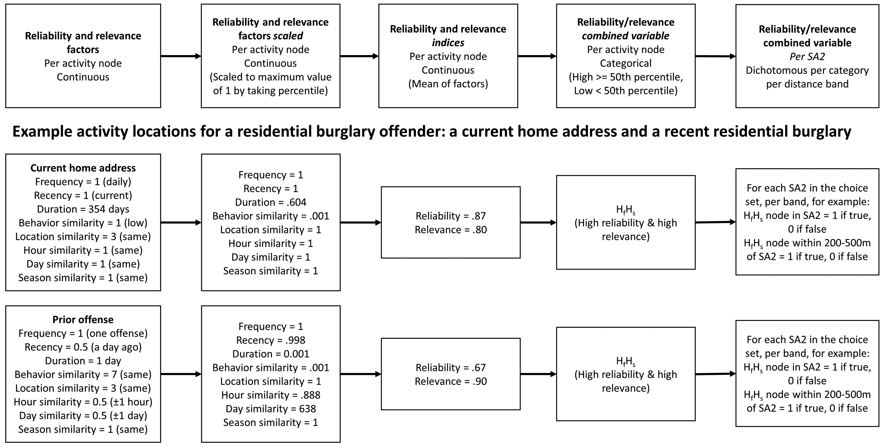
Overview and examples of the process for constructing the prior activity location variables.

First, reliability and relevance variables (e.g., recency, behavior similarity) were calculated for each prior activity node, as summarized in Table 1 and further detailed in Supplemental Material S1. Where variables were absent in the data, we applied reasonable assumptions about the typical timing and nature of people's activities at different nodes. For example, all home nodes were coded as maximal time of day and day of week similarity to the reference offense because people have typically been at their homes at all times of day and week. Home nodes were also coded as low behavioral similarity to the reference offense given people's most common activities at home do not include burglary, robbery, or sex offences against non-family members. Where multiple node types fell at the same location (coordinates), occurring for 15% of locations, we took the maximum of each variable on the grounds that this would best represent the person's knowledge reliability and relevance for that location. All variables were then re-scaled so that a value of 1 represented maximal frequency, recency, duration, and similarity (i.e., 100th percentile out of all offenders’ activity locations in the dataset for each crime type model).

Table 1.

Reliability and Relevance Variable Construction Summary.

Factor	Definition	Coding rules
Frequency (0 to 1)	Proportion of days over the offender's association with a given node that it was visited	Home: daily = 1 Family members’ homes: fortnightly = 0.07 School/education: 200 days per year = 0.55 Work: 240 days per year = 0.66 Events: number of events at location/duration.
Recency (0 to 1)	Reciprocal of the number of days between reference offense and most recent activity at the node.	Time-span nodes: used latest end date of all records for that node (e.g., home address). Events: used date of latest event.
Duration (0 to max duration)	Number of days between earliest and latest date at the node.	Time-span nodes: earliest start date to latest end date of all records for that node (e.g., home address). Events: date of first event to date of latest event.
Behavior similarity (1 to 7)	Ordinal scale of similarity based on Kuang et al.'s (2017) study of the similarity of different crimes (see Supplemental Material S1).	7 Prior crime of same crime type
		6 Prior crime of similar crime type
		5 Prior crime of not similar crime type
		4 Prior crime experienced as a victim/witness, of same crime type
		3 Prior crime or incident experienced as a victim/witness, of similar type
		2 Prior crime or incident experienced as a victim/witness, of not similar type
		1 Other activity node (all other nodes)
Location similarity (1 to 3)	Ordinal scale of similarity between activity node and reference offense^a	3 Same location type
		2 Unknown similarity
		1 Different location type
Hour similarity (0 to 1)	Reciprocal of the difference in hours between reference offense hour of the day and activity hour of the day.	Home & family members’ homes: any time of day. School/education: 08:00–16:00. Work: 08:00–18:00. Events: time of the event.
Day similarity (0 to 1)	Reciprocal of the difference in days between reference offense day of the week and activity day of the week.	Home & family members’ homes: any day. School/education & work: Monday to Friday. Events: day of the event.
Season similarity (0 to 1)	Reciprocal of the difference in seasons between reference offense season and activity season.	Time-span nodes: if time span covered the same season as reference offense, 1, else take the minimum difference in seasons to season of time span start date or end date. Events: minimum difference to event season.

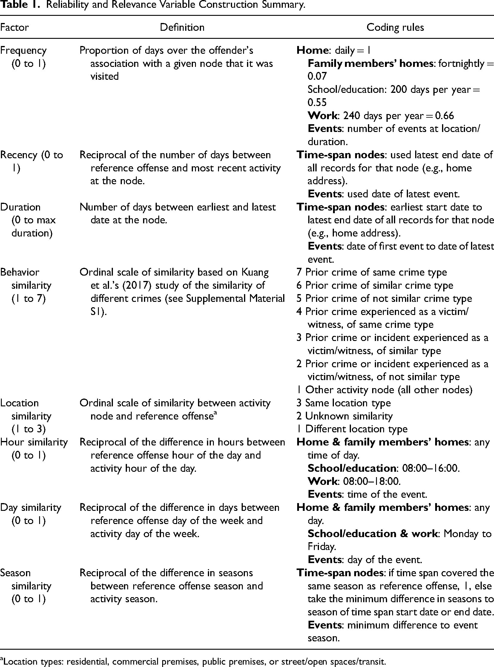
^aLocation types: residential, commercial premises, public premises, or street/open spaces/transit.

Second, we averaged the reliability variables (frequency, recency, and duration) and relevance variables (behavior, location type, hour, day, and season similarity) to create indices representing the latent constructs of reliable and relevant knowledge. We used all variables following preliminary analyses exploring whether each explained additional variance and were not therefore redundant (see Supplemental Material S1). We weighted each variable equally in the absence of a priori guidance as to the relative importance of each variable to reliability and relevance (a topic that future research could explore). Reflecting the theoretical model, activity locations that were visited frequently, recently and over a longer period of time had high reliability scores; activity locations with high similarity on multiple similarity dimensions had high relevance scores.

Third, we combined the indices into a categorical variable reflecting H1(a) to (c), based on whether the activity node was “high” (greater or equal to the 50th percentile) or “low” (below the 50th percentile) on each index. Activity locations with high reliability (familiarity) and high relevance (similarity) were coded H_fH_s (where subscript f = familiarity/reliability and s = similarity/relevance), those with high reliability and low relevance H_fL_s, low reliability and high relevance L_fH_s, and low reliability and low relevance L_fL_s.⁵

Dichotomizing and combining the reliability and relevance indices in this way provided various benefits over interacting the continuous indices. The resulting categories are easy to interpret, directly map to H1(a) to (c) and could be combined with distance categories to examine distance decay as described below. Dichotomized “high” and “low” categories also enabled comparison with the qualitatively different category “no reliable or relevant knowledge” (absence of any activity node) that forms the reference category. Creating categorical variables that combine activity location attributes in this way is common in DSCM studies (e.g., recency×duration: Bernasco, 2010a; Lammers et al., 2015; time of day×day of week×prior offense type similarity: van Sleeuwen et al., 2018).

Naturally, these categories are strongly related to node type, though there was variation. For example, most home nodes were categorized as H_fH_s, reflecting that home is a high frequency activity location of typically long duration, visited at any time or day or week, resulting in above average reliability and relevance indices in most (but not all) cases. Family homes were more evenly divided across categories but were the most common node type in the H_fH_s category due to their volume, with prior offenses the third most prevalent node type in the H_fH_s category (though of much smaller number overall). Prior offense and other event-based nodes were roughly evenly split between H_f and L_f—though predominantly L_s reflecting lower temporal similarity. A full comparison of node type and reliability/relevance category is provided in Supplemental Material Table S2.2.

Last, each SA2 (in each offender's set) was coded based on the presence (1) or absence (0) of at least one of each type of activity node (H_fH_s / H_fL_s / L_fH_s / L_fL_s). Each SA2 was then also coded based on the presence (1) or absence (0) of activity nodes outside the SA2 at a series of distance bands, being: between 0 and 200 m outside the SA2 boundary, then 200–500 m, 500m–1 km, 1–2 km, and 2–5 km. Only the activity nodes in the distance band containing the nearest activity node(s) were included. For example, if there were no activity nodes in the SA2, but there was an H_fH_s node and an L_fL_s node within 0–200 m, the variables “H_fH_s node 0–200m” and “L_fL_s node within 0–200m” were coded 1 and all remaining variables (e.g., “H_fH_s node in SA2,” “L_fH_s node within 200–500m,” and so on) were coded 0. This approach is equivalent to dummy coding the distance to the nearest node of each category and is consistent with previous studies (e.g., Menting et al., 2020). It enables examination of patterns of distance decay over increasing distances-to-nearest-nodes, a benefit over using continuous distance and information about more distant nodes. The reference category for each variable (e.g., H_fH_s node within SA2, L_fH_s node 200–500 m from the SA2) is no node within 5 km of the SA2—indicating a lack of knowledge of the SA2 in the absence of any nearby activity node.

Opportunity (Control) Variables

Opportunity variables were derived from NZ Statistics Census and Business Demography data (http://nzdotstat.stats.govt.nz/). Consistent with past DSCM research, these variables represent, directly or indirectly, the number of targets (or an indicator thereof) per SA2. For each crime type (i.e., each model), we included a single variable indicative of the target or victim distribution for that crime type.

For crimes targeting particular types of premises—residential burglary, non-residential burglary, and commercial robbery—the opportunity measures directly captured the number of those types of premises per SA2 (as per Bernasco & Nieuwbeerta, 2005; Frith, 2019; Townsley et al., 2015). These were: number of households for residential burglary; number of business units in any industry for non-residential burglary; and the number of business units in commercial industries (e.g., retail, accommodation, and food services) that matched the types of premises used to identify commercial robbery (the “commercial” location types described in relation to the location similarity variable above).

For personal robbery and sex offenses, we used the number of business units in commercial or public industries (as for commercial robbery plus industries such as transport, education, and health care). This variable served as an indirect indicator of ambient population, which is a better measure of the target distribution than residential population, for personal robbery and other offenses targeting people rather than premises (Andresen, 2011; Andresen & Jenion, 2010; Rummens et al., 2021). See Supplemental Material S1 for further detail.

Analytic Approach

As with most previous DSCM studies, we employed conditional logit models (McFadden, 1984). The mechanics of the conditional logit model are described in detail elsewhere (Bernasco, 2010b), but to summarize, the model estimates the expected utility of each choice alternative (SA2), given the attributes of that alternative, and selects the alternative that maximizes utility. It yields the estimated probability that an offender will choose an alternative, given its attributes and parameters representing the effects of these attributes on the decision, estimated in such a way as to make the modeled choices match the observed choices as closely as possible.

We exponentiate these estimated parameters to report them as odds ratios (ORs). The ORs indicate the increase/decrease in the odds of an offender choosing an SA2 given the presence of an activity node with a given attribute (e.g., activity node with high reliability and high relevance within 0–200 m of the SA2) relative to there being no activity node within 5 km of the SA2. For the opportunity covariates, the ORs represent the change in odds for each 100 unit increase in households or businesses.

For each crime type we ran a conditional logit model involving four reliability-relevance categories (H_fH_s, H_fL_s, L_fH_s, L_fL_s)×6 distance bands (within SA2 plus 5 outside) + 1 opportunity variable = 25 estimates. We tested H1(a) to (c) with Wald's Chi-Square difference tests comparing the ORs for H_fH_s versus H_fL_s and L_fH_s, and H_fL_s and L_fH_s versus L_fL_s, within each distance band. Supplemental Material S2 provides descriptive statistics showing the proportion of all sampled SA2s with nodes of each category (H_fH_s to L_fL_s) in each distance band, and summarizing the opportunity variables.

Results

The results are illustrated in Figure 2, which displays the 95% confidence intervals around the ORs. The exact statistics and Wald tests statistics are reported in Supplemental Materials S3 and S4, respectively. Table 2 provides the model summary statistics for each crime type. The Pseudo R² values, ranging from 0.27 to 0.36, indicate a good fit to the data (McFadden, 1973) and are comparable with previous DSCM studies.

Figure 2.

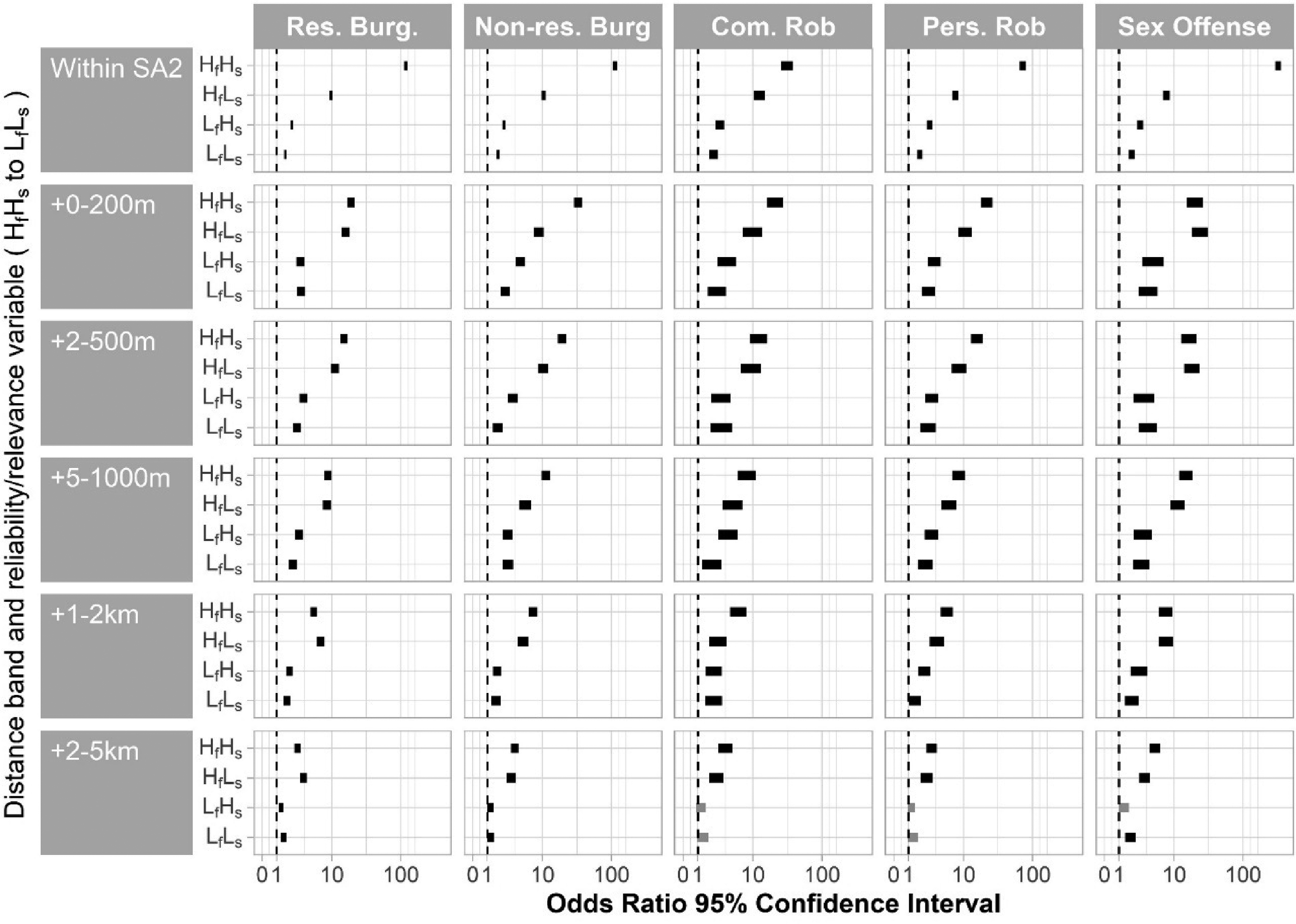
Odds ratio 95% confidence intervals for reliability and relevance variables per distance band for each model (crime type). The shorter the bar, the smaller the CI. Non-significant associations have CIs that cross the vertical line at 1 and are gray. ORs with bars that do not overlap are significantly different. ORs with bars that overlap may be significantly different: see Wald tests results in Supplemental Material S4. In “H_fL_s,” H = high, L = low, f = familiarity/reliability, and s = similarity/relevance.

Table 2.

Model Summary Statistics.

Statistic	Res. Burg.	Non-Res. Burg.	Com. Rob.	Pers. Rob.	Sex offenses
N offense choices	17,054	10,353	1,977	4,315	4,421
N SA2 choice alternatives	4,213,998	2,417,735	563,161	1,243,204	784,537
Pseudo R²	0.35	0.36	0.27	0.31	0.32

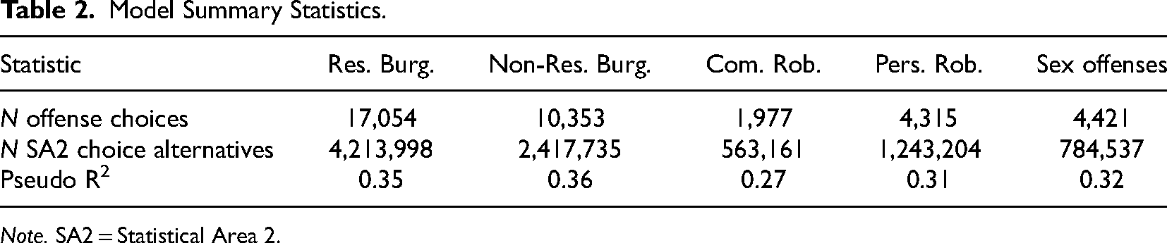
Note. SA2 = Statistical Area 2.

Supporting H1(a) and H1(b), for all crime types, the presence of an H_fH_s node was significantly more likely to result in an SA2 being chosen than the presence of H_fL_s or L_fH_s nodes. The latter in turn were significantly more likely to be chosen than SA2s containing L_fL_s nodes—supporting H1(c), except for commercial robbery where the Wald test for L_fH_s versus L_fL_s was not significant. However, the difference in point estimates for commercial robbery was in the hypothesized direction, and the width of the confidence intervals suggest the sample size for commercial robbery was too small to reliably test this difference given the number of variables in the model—so we do not consider the result reason to reject H1(c).

The hypothesized differences were most pronounced in the “within SA2” distance band, with fewer significant differences when the nearest activity nodes were farther away. H_fH_s versus L_fH_s (H1(b)) and H_fL_s versus L_fL_s (H1(c)) differences were significant and in the hypothesized direction for all 25 comparisons outside the “same SA2” band, H_fH_s versus H_fL_s for 11 (H1(b)), and L_fH_s versus L_fL_s for 4 (H1(c)). In one instance the results were significant in the opposite direction to the hypothesis (for residential burglary and the 1–2 km distance band, H_fL_s> H_fH_s: H1(b)). We approach exceptions to the hypothesized trend at longer distance bands with caution: they could be a product of coding for typical node timing and similarity where we did not have specific data. Any error introduced by this imprecision would be most consequential at greater distances, where we expect (and find) weaker associations between activity nodes and crime location choice.

As expected, a pattern of distance decay, or a decline in the odds of crime location choice with increasing distance bands, is exhibited in Figure 2. Compare, for example, the ORs for H_fH_s nodes (the top-most point in each box) over the distance band boxes down the residential burglary column. We likewise found, as expected, significant positive associations between crime location choice and the opportunity covariates. For every 100 units (e.g., households, commercial premises) in the SA2, the odds of crime increased by a factor of 1.06 for residential burglary (95% CI: 1.05–1.06), 1.11 for non-residential burglary (1.10–1.11), 1.11 for commercial robbery (1.10–1.12), 1.11 for personal robbery (1.10–1.11), and 1.08 for sex offenses (1.07–1.09).

Discussion

This study aimed to advance our ability to explain and predict where individual offenders will commit crime, by testing the hitherto untested contributions of the reliability and relevance constructs theorized in the model proposed by Curtis-Ham et al. (2020). Specifically, we tested whether offenders are more likely to commit crime in locations where their prior activities have generated both reliable and relevant knowledge of crime opportunities. The general pattern of results—supporting H1(a) to (c)—was that offenders were more likely to commit crime near to activity nodes that were high on both reliability and relevance, lower in proximity to activity nodes that were high on only reliability or relevance and lowest in proximity to activity nodes that were low on both reliability and relevance. In other words, crime was most likely at locations with which offenders were more familiar and at which they had conducted more similar activities in the past, and least likely at locations with which offenders were less familiar and where they had conducted less similar activities. These results support the theorized combined effect of familiarity and similarity, advancing on previous studies which had only explored isolated activity location attributes.

An alternative explanation for the findings is that people are simply more likely to be caught for crimes committed near high reliability/high relevance activity nodes than for crimes committed near low reliability or low relevance nodes. In other words, because we only studied solved crimes, the results are confounded by an unmeasured variable reflecting the rate at which police solve crimes committed near activity nodes with different levels of reliability and relevance. However, studying offenses linked by DNA to both identified (caught) and unidentified offenders, Lammers (2014) found that people who offended near past crimes—high relevance nodes—were not more likely to get caught, or caught sooner, than people whose offenses were farther apart. Similarly, Bernasco et al. (2013) found no or weak correlations between robbery detection rates and a range of environmental features that represent common activity locations (e.g., bars, restaurants, retail outlets). Further, several studies using survey data on self-reported crimes—both detected by police and undetected—have found relationships between the frequency (Menting et al., 2020) and timing (van Sleeuwen et al., 2021) of past visits to locations and future crime locations that are consistent with studies of frequency and timing using solved crime data (Bernasco, 2019; van Sleeuwen et al., 2018). It is therefore unlikely that offenders’ probability of detection covaries with reliability and relevance factors to an extent that would produce our results.

Another alternative explanation is that offenders are more likely to have high reliability/high relevance activity nodes in places with more crime opportunities and thus the results reflect the underlying opportunity structure, rather than individual offenders’ activities. We controlled for the distribution of opportunities using measures that reflected the distribution of potential crime targets for each crime type. But it remains possible that other unmeasured aspects of the environment that are conducive to both crime and activities that generate reliable and relevant knowledge could explain some of the variance we attribute to those activities. Particularly with recent prior crimes of the same type—which could be high reliability and high relevance—it may be difficult to disentangle the effect of existing opportunities from the effect of knowledge gained from previously exploiting those opportunities. However, research on repeat and near repeat offending supports our interpretation of the results: a “boost” effect—from the highly reliable and relevant knowledge gained from a recent crime—explains offenders’ tendency return to prior crime locations beyond the effect of opportunity structure alone (Bowers & Johnson, 2004; Lantz & Ruback, 2017).

The present findings build on prior studies that employed DSCMs to study individual reliability and relevance variables in isolation (e.g., Bernasco, 2019; Ruiter, 2017; van Sleeuwen et al., 2021), by demonstrating how these variables operate collectively. This combined effect had only been hinted at by previous findings that offenders are much more likely to commit crime near their current homes—a high reliability, high timing similarity activity node—(Bernasco, 2010a; Lammers et al., 2015) and places they have committed multiple or recent offenses of the same type and/or at the same period of the week (Lammers et al., 2015; van Sleeuwen et al., 2018), than near other activity nodes.

The pattern of declining likelihood of crime with increasing distance—clearest for the high reliability/high relevance activity locations—is also consistent with previous studies (Bernasco, 2019; Bernasco & Block, 2009; Kuralarasan & Bernasco, 2021; Menting et al., 2020). However, a novel finding is that this distance decay pattern was flatter and not always monotonic in relation to activity locations lower on either or both dimensions, implying that people are just as unlikely to commit crime close to low reliability or low relevance activity locations as farther away from them (but still within 5 km).

That the opportunity variables were also associated with crime location choice when controlling for the presence and attributes of offenders’ activity locations is also consistent with previous literature. Past DSCM studies typically only included offenders’ homes and one or two other nodes (e.g., family members’ homes, prior crimes), enabling only partial control for offenders’ activity locations (e.g., Lammers et al., 2015; Menting et al., 2016; van Sleeuwen et al., 2018). However, similar opportunity effects were also observed by Bernasco (2019) and Menting et al. (2020) when controlling for a wide range of activity locations. That people offend where there are more opportunities regardless of whether they have an activity location nearby could reflect activity locations missing from the data, awareness of opportunities generated through processes other than direct experience, or offending outside of awareness space (Curtis-Ham et al., 2020).

Our findings broaden the empirical evidence base for crime pattern theory (Brantingham & Brantingham, 1991, 1993a) and its extension in the model proposed by Curtis-Ham et al. (2020) in several ways. First, by including all attributes of activity locations from the model—previously only studied in isolation—our findings provide the first evidence of the theorized roles of reliable and relevant location knowledge in offenders’ crime location choices. They highlight the importance of including both the quantitative (reliability) and qualitative (relevance) attributes of offenders’ activity locations when examining their crime location choices in research or practice.

Second, the findings demonstrate the salience of a broad range of activity locations to offenders’ crime location choices. We included a variety of different activity locations and observed strong associations between proximity to activity locations—particularly those with high reliability and relevance—and offenders’ crime locations. Much of the individual-level research on crime pattern theory has focused on offenders’ current homes as a proxy for their awareness space (Ackerman & Rossmo, 2015; Ruiter, 2017; Townsley, 2016). However, the present study corroborates—on a much larger scale—previous small-scale and qualitative studies that suggested that many activity locations other than home play an important role generating awareness of crime opportunities (e.g., Bernasco, 2019; Costello & Wiles, 2001; Davies & Dale, 1996; Menting et al., 2020; Wright & Decker, 1994), consistent with the original formulation of crime pattern theory by the Brantinghams (1991, 1993a).

Third, by including a range of crimes reflecting different types of targets and motivations and analyzing them separately, this study lends support to the generalizability of both crime pattern theory, and Curtis-Ham et al.'s extension, to different crimes. Previous studies have tended to study a wide range of crimes in combination (e.g., Lammers et al., 2015; Menting et al., 2016) or to focus on a single crime type (e.g., Frith et al., 2017; Kuralarasan & Bernasco, 2021; Long et al., 2018; c.f. Bernasco, 2010a; Frith, 2019). The former studies are likely to have masked crime specific patterns, with the results simply reflecting high volume crime types; the latter studies leave questions about the generalizability of their findings across crime types. The present study overcame both these limitations. Importantly, the consistency of the observed pattern for reliability and relevance across crime types indicates that it likely generalizes beyond the crimes included in this study. That said, we recommend future studies expand the range of crimes included, to test this suggestion empirically, using both police data and other sources (discussed further below). From a methodological perspective, it would be informative to explore whether the results generalize to crime types where the spatial distribution—in police data—is heavily influenced by variations in reporting or proactive policing (e.g., disorder and drug offenses).

An additional implication of the separate crime type analyses is that the consistency across crimes supports the generalizability of the results beyond the analyzed samples. The use of a dataset from a hitherto understudied part of the world also adds support to the generalizability of crime pattern theory, and its recent extension, across crime behaviors and contexts.

An unexpected finding of potential theoretical significance was the smaller difference between L_fH_s and L_fL_s activity nodes than between H_fL_s and L_fL_s activity nodes. The lack of distinction between low reliability/high relevance and low reliability/low relevance activity locations indicates that if offenders are less familiar with a location, the nature of their previous activities there matters less. In other words, there appears a notional minimum amount of reliable location knowledge below which relevance does not matter. Conversely, once a threshold level of familiarity is reached, the behavior, type of location and timing involved in offenders’ prior activities in a location make a greater difference to whether they ultimately choose to offend nearby. This interpretation is speculative, however, and warrants replication with other datasets and methods.

In terms of methodology, the foregoing findings highlight the utility of DSCM as a method for quantifying relationships between attributes of offenders’ activity locations and their crime locations. They also demonstrate that police data can yield useful insights into these relationships, through the inclusion of a wide range of activity locations beyond just home and prior crime locations as previously studied. However, our results should be interpreted in light of several limitations which illustrate the challenges involved in operationalizing these attributes using police administrative data, within the DSCM paradigm.

First, our measures of reliability and relevance—constructed by combining attributes of offenders’ activity locations—were proxies for offenders’ knowledge; we did not assess their knowledge directly. Although it is common in discrete choice research to analyze people's preferences through behavioral proxies for their internal decision-making processes (Bernasco, 2017), the words “knowledge” and “familiarity” as used in this paper should be interpreted as short-hand for “knowledge/familiarity as inferred from observed behavior.” It nonetheless constitutes a major improvement over previous studies where the only measures of spatial knowledge are proximity to a single activity location (e.g., home) or a single behavioral attribute such as frequency of visits.

Second, our method for filling in missing data in the reliability and relevance variables necessarily introduced some imprecision. For example, we used the average frequency and timing of visits to family members (from a time-use survey), because the data did not measure individual visits, and applied a simple scale for behavioral similarity, because the data lacked detail about the activities conducted at some activity locations (e.g., the “other police contacts”). Frequency was likely overestimated for activity locations such as prior offenses and other event-based nodes where police records only capture a single visit to a location (see Supplemental Material S1). Considering these sources of error, in drawing conclusions we put more emphasis on the general pattern, seen consistently across the crime types, than the specific effect sizes observed.

Further research could supplement the present findings using complementary methods that overcome the above limitations. For example, in-depth interviews could be used to investigate offenders’ perceived familiarity with locations and similarity of prior activities to a given crime, and the relative roles of these constructs in the decision where to commit that crime. Time-use surveys could overcome the inherent lack of completeness and detail in police records by capturing the timing, location, and behavior involved in offenders’ pre-offense activities with greater precision and detail. Survey methods could also extend on recent survey based DSCM studies by explicitly including the reliability and relevance variables, though sample sizes would need to be increased considerably (Bernasco, 2019; Menting et al., 2020; van Sleeuwen et al., 2021). Given more detailed descriptions of the behavior involved in offenders’ reference offenses and prior activities, similarity could be measured on a range of dimensions (see Farrell, 2015), or through text analysis (e.g., Birks et al. 2020; Kuang et al., 2017). Our interpretation of the observed patterns for reliability and relevance could also be corroborated by future research including a wider range of opportunity variables to better isolate the effects of opportunities versus activities, examining other crime types, and seeing if the threshold effect appears in other jurisdictions.

Another avenue for future research in continuing the empirical investigation of Curtis-Ham et al.'s (2020) model, would be to consider different subgroups of offenders. For example, separating sex offenders by victim age or by their relationship to victim might reveal differences masked in the present dataset (which did not include such victim information). Given individual differences in risk tolerance (Palminteri & Chevallier, 2018), and differences in criminal expertise and offending styles (Brantingham et al., 2020; Nee, 2015; Sanders et al., 2016), it is plausible that some offenders would prefer to commit crime in very familiar places where their prior activities have generated readily transferrable knowledge, while others would be more likely to seize crime opportunities despite a relative lack of reliable and relevant knowledge of the location.

We conclude by highlighting the practical implications of the present study. Firstly, understanding the combined contribution of reliability and relevance is important for informing predictions about where individual offenders are likely to offend, which in turn can inform crime prevention and investigation strategies. Our results suggest that both reliability and relevance factors should be included when making such predictions about where individuals will offend. People are most likely to offend in places that they know well—as indicated, collectively, by the frequency, recency, and duration of their activities in those places—and that their activities have been most conducive to acquiring relevant knowledge of crime opportunities—as indicated by the similarity in behavior, type of location, and timing involved. Practitioners conducting geographic profiling (Rossmo, 2000) in police investigations could apply these factors to assess suspects’ likelihood of having committed a crime given the location and attributes their nearby activity locations, and prioritize the suspects accordingly (e.g., Curtis-Ham et al., 2022a). Practitioners working with offenders in the community could apply these factors to identify offenders’ highest risk locations for re-offending and devise plans to manage the risk such locations present.

Second, there are implications for understanding and responding to crime in the aggregate. The theoretical framework tested in this paper, particularly the concepts of reliability and relevance, could be used when analyzing aggregate crime patterns. For example, a crime hotspot is a product of opportunities in the awareness space of many offenders (Brantingham & Brantingham, 1991), so when examining a given hotspot, one might ask: what nearby offender activity locations are providing reliable and relevant knowledge of those opportunities? Understanding how opportunity and collective familiarity and activity similarity are interacting to produce crime could help inform more nuanced interventions.

In sum, by simultaneously accounting for the various activity location attributes theorized to affect crime location choice and using a large administrative dataset with a wide array of activity locations, we provide the first empirical evidence of the joint importance of both reliable and relevant knowledge to offenders’ crime location choices. Our findings add to the empirical evidence base for crime pattern theory and its recent extension by Curtis-Ham et al. (2020). By advancing our understanding of the kinds of places that people are more likely to commit crime, this research enhances our ability to predict where people will offend—individually and collectively, with important implications for crime prevention and investigation.

Supplemental Material

sj-pdf-1-icj-10.1177_10575677241244464 - Supplemental material for Familiar Locations and Similar Activities: Examining the Contributions of Reliable and Relevant Knowledge in Offenders’ Crime Location Choices

Supplemental material, sj-pdf-1-icj-10.1177_10575677241244464 for Familiar Locations and Similar Activities: Examining the Contributions of Reliable and Relevant Knowledge in Offenders’ Crime Location Choices by Sophie Curtis-Ham, Wim Bernasco, Oleg N. Medvedev and Devon L. L. Polaschek in International Criminal Justice Review

Footnotes

Acknowledgments

We gratefully acknowledge the assistance of the NZ Police staff who provided access to and advice on the data used in this research and who reviewed the manuscript prior to submission. We also thank all who reviewed this paper and provided constructive feedback that helped improve it.

Declaration of Conflicting Interests

The first author is employed as a researcher at New Zealand Police. This study was not conducted as a part of that employment..

Ethics Approval

This research study was conducted retrospectively from data obtained for operational purposes. Ethics approval was obtained from the Psychology Research and Ethics Committee of the University of Waikato (reference #19:13). Approval of access to data for this study was obtained from the NZ Police Research Panel (reference EV-12-462). The results presented in this paper are the work of the authors and do not represent the views of New Zealand Police.

Funding

The authors disclosed receipt of the following financial support for the research, authorship, and/or publication of this article: This research formed part of the first author's PhD thesis, which was funded by a University of Waikato doctoral scholarship.

ORCID iDs

Sophie Curtis-Ham

Wim Bernasco

Supplemental Material

Supplemental material for this article is available online.

Notes

Author Biographies

Sophie Curtis-Ham, PhD, is an honorary research associate at the University of Waikato and senior researcher at New Zealand Police. She has previously worked as an intelligence analyst in the UK and NZ. Her research interests span the fields of evidence-based policing, investigative and forensic psychology and environmental criminology, and her PhD research focused on leveraging offender activity location data to enhance geographic profiling in criminal investigations.

Wim Bernasco, PhD, is a senior researcher at the Netherlands Institute for the Study of Crime and Law Enforcement (NSCR) and a Professor in the Department of Spatial Economics at the Vrije Universiteit Amsterdam. His research interests include the geography of crime, offenders’ target selection, and situational causes of offending and victimization, including the behavioral analysis of crimes caught on CCTV.

Oleg N. Medvedev, PhD, is assistant professor at the University of Waikato and associate editor of journal Mindfulness. He teaches advanced research programmes and his research involves the development and application of advanced statistical methodology. He is an author on over 50 journal articles and book chapters and co-author of the book Mindfulness-Based Intervention Research: Characteristics, Approaches, and Developments.

Devon L. L. Polaschek, PhD, DipClinPsyc, is a professor of psychology in the School of Psychology and Director of the New Zealand Institute of Security and Crime Science, University of Waikato, New Zealand. Her research interests include theory, intervention, and intervention evaluation with serious violent and sexual offenders, family violence, psychopathy, desistance, reintegration, and parole.

References

Ackerman

J. M.

Rossmo

D. K.

(2015). How far to travel? A multilevel analysis of the residence-to-crime distance. Journal of Quantitative Criminology, 31(2), 237–262. https://doi.org/10.1007/s10940-014-9232-7

Andresen

M. A.

(2011). The ambient population and crime analysis. The Professional Geographer, 63(2), 193–212. https://doi.org/10.1080/00330124.2010.547151

Andresen

M. A.

Jenion

G. W.

(2010). Ambient populations and the calculation of crime rates and risk. Security Journal, 23(2), 114–133. https://doi.org/10.1057/sj.2008.1

Ben-Akiva

M. E.

Lerman

S. R.

(1985). Discrete choice analysis: Theory and application to travel demand. MIT Press.

Bernasco

(2010a). A sentimental journey to crime: Effects of residential history on crime location choice. Criminology; An Interdisciplinary Journal, 48(2), 389–416. https://doi.org/10.1111/j.1745-9125.2010.00190.x

Bernasco

(2010b). Modeling micro-level crime location choice: Application of the discrete choice framework to crime at places. Journal of Quantitative Criminology, 26(1), 113–138. https://doi.org/10.1007/s10940-009-9086-6

Bernasco

(2017). Modeling offender decision making with secondary data. In Bernasco

Van Gelder

J.-L.

Elffers

(Eds.), The Oxford handbook on offender decision making (pp. 569–586). Oxford University Press.

Bernasco

(2019). Adolescent offenders’ current whereabouts predict locations of their future crimes. PLOS ONE, 14(1), e0210733. https://doi.org/10.1371/journal.pone.0210733

Bernasco

Block

(2009). Where offenders choose to attack: A discrete choice model of robberies in Chicago. Criminology, 47(1), 93–130. https://doi.org/10.1111/j.1745-9125.2009.00140.x

10.

Bernasco, W., Block, R., & Ruiter, S. (2013). Go where the money is: Modeling street robbers' location choices. Journal of Economic Geography, 13(1), 119–143. https://doi.org/10.1093/jeg/lbs005

11.

Bernasco

Johnson

S. D.

Ruiter

(2015). Learning where to offend: Effects of past on future burglary locations. Applied Geography, 60(Supplement C), 120–129. https://doi.org/10.1016/j.apgeog.2015.03.014

12.

Bernasco

Kooistra

(2010). Effects of residential history on commercial robbers’ crime location choices. European Journal of Criminology, 7(4), 251–265. https://doi.org/10.1177/1477370810363372

13.

Bernasco

Nieuwbeerta

(2005). How do residential burglars select target areas? A new approach to the analysis of criminal location choice. The British Journal of Criminology, 45(3), 296–315. https://doi.org/10.1093/bjc/azh070

14.

Bernasco

Ruiter

Block

(2017). Do street robbery location choices vary over time of day or day of week? A test in Chicago. Journal of Research in Crime and Delinquency, 54(2), 244–275. https://doi.org/10.1177/0022427816680681

15.

Birks

Coleman

Jackson

(2020). Unsupervised identification of crime problems from police free-text data. Crime Science, 9(1), 1–19. https://doi.org/10.1186/s40163-020-00127-4

16.

Bowers

Johnson

(2004). Who commits near repeats? A test of the boost explanation. Western Criminology Review, 5(3), 12–24.

17.

Brantingham

P. J.

Brantingham

P. L.

Song

Spicer

(2020). Crime hot spots, crime corridors and the journey to crime: An expanded theoretical model of the generation of crime concentrations. In Lersch

K. M.

Chakraborty

(Eds.), Geographies of behavioural health, crime, and disorder (Vol. 126, pp. 61–86). Springer.

18.

Brantingham

P. L.

Brantingham

P. J.

(1991). Notes on the geometry of crime. In Brantingham

P. J.

Brantingham

P. L.

(Eds.), Environmental criminology (pp. 27–54). Waveland Press.

19.

Brantingham

P. L.

Brantingham

P. J.

(1993a). Environment, routine, and situation: Toward a pattern theory of crime. In Clarke

R. V.

Felson

(Eds.), Routine activity and rational choice, advances in criminological theory (pp. 259–294). Transaction Publishers.

20.

Brantingham

P. L.

Brantingham

P. J.

(1993b). Nodes, paths and edges: Considerations on the complexity of crime and the physical environment. Journal of Environmental Psychology, 13(1), 3–28. https://doi.org/10.1016/S0272-4944(05)80212-9

21.

Bruinsma

G. J. N.

Johnson

S. D.

(eds) (2018). The oxford handbook of environmental criminology. Oxford University Press.

22.

Clare

Fernandez

Morgan

(2009). Formal evaluation of the impact of barriers and connectors on residential Burglars’ macro-level offending location choices. Australian & New Zealand Journal of Criminology, 42(2), 139–158. https://doi.org/10.1375/acri.42.2.139

23.

Cohen

L. E.

Felson

(1979). Social change and crime rate trends: A routine activity approach. American Sociological Review, 44(4), 588–608. https://doi.org/10.2307/2094589

24.

Costanzo

Halperin

Gale

(1986). Criminal mobility and the directional component in journeys to crime. In Figlio

Hakim

Rengert

(Eds.), Metropolitan crime patterns (pp. 73–96). Criminal Justice Press.

25.

Costello

Wiles

(2001). GIS And the journey to crime: An analysis of patterns in south yorkshire. In Bowers

K. J.

Hirschfield

(Eds.), Mapping and analysing crime data: Lessons from research and practice (pp. 27–60). Taylor & Francis.

26.

Curtis-Ham

Bernasco

Medvedev

O. N.

Polaschek

D. L. L.

(2021a). A national examination of the spatial extent and similarity of offenders’ activity spaces using police data. ISPRS International Journal of Geo-Information, 10(2), 47. https://doi.org/10.3390/ijgi10020047

27.

Curtis-Ham

Bernasco

Medvedev

O. N.

Polaschek

D. L. L.

(2022a). A new Geographic Profiling Suspect Mapping and Ranking Technique for crime investigations: GP-SMART. Journal of Investigative Psychology and Offender Profiling, 19(3), 103–117. https://doi.org/10.1002/jip.1585 .

28.

Curtis-Ham

Bernasco

Medvedev

O. N.

Polaschek

D. L. L.

(2022b). Relationships between offenders’ crime locations and different prior activity locations as recorded in police data. Journal of Police and Criminal Psychology, 38, 172–183. https://doi.org/10.1007/s11896-022-09540-8

29.

Curtis-Ham

Bernasco

Medvedev

O. N.

Polaschek

D. L. L.

(2020). A framework for estimating crime location choice based on awareness space. Crime Science, 9(1), 1–14. https://doi.org/10.1186/s40163-020-00132-7

30.

Curtis-Ham

Bernasco

Medvedev

O. N.

Polaschek

D. L. L.

(2021b). The importance of importance sampling: Exploring methods of sampling from alternatives in discrete choice models of crime location choice. Journal of Quantitative Criminology, 38, 1003–1031. https://doi.org/10.1007/s10940-021-09526-5

31.

Davies

Dale

(1996). Locating the stranger rapist. Medicine, Science and the Law, 36(2), 146–156. https://doi.org/10.1177/002580249603600210

32.

Farrell

(2015). Crime concentration theory. Crime Prevention & Community Safety, 17(4), 233–248. https://doi.org/10.1057/cpcs.2015.17

33.

Frith

M. J.

(2019). Modelling taste heterogeneity regarding offence location choices. Journal of Choice Modelling, 33, 100187. https://doi.org/doi.org/10.1016/j.jocm.2019.100187

34.

Frith

M. J.

Johnson

S. D.

Fry

H. M.

(2017). Role of the street network in Burglars’ spatial decision-making. Criminology, 55(2), 344–376. https://doi.org/10.1111/1745-9125.12133

35.

Hillier

Smith

Cannuscio

C. C.

Karpyn

Glanz

(2015). A discrete choice approach to modeling food store access. Environment and Planning B, Planning & Design, 42(2), 263–278. https://doi.org/10.1068/b39136

36.

Kuang

Brantingham

P. J.

Bertozzi

(2017). Crime topic modeling. Crime Science, 6(1), 1–20. https://doi.org/10.1186/s40163-017-0074-0

37.

Kuralarasan

Bernasco

(2021). Location choice of snatching offenders in Chennai city. Journal of Quantitative Criminology, 38(3), 673–696. https://doi.org/10.1007/s10940-021-09514-9 .

38.

Lammers

(2014). Are arrested and non-arrested serial offenders different? A test of spatial offending patterns using DNA found at crime scenes. Journal of Research in Crime and Delinquency, 51(2), 143–167. https://doi.org/10.1177/0022427813504097

39.

Lammers

(2018). Co-offenders’ crime location choice: Do co-offending groups commit crimes in their shared awareness space? The British Journal of Criminology, 58(5), 1193–1211. https://doi.org/10.1093/bjc/azx069 .

40.

Lammers

Menting

Ruiter

Bernasco

(2015). Biting once, twice: The influence of prior on subsequent crime location choice. Criminology, 53(3), 309–329. https://doi.org/10.1111/1745-9125.12071

41.

Lantz

Ruback

R. B.

(2017). A networked boost: Burglary co-offending and repeat victimization using a network approach. Crime & Delinquency, 63(9), 1066–1090. https://doi.org/10.1177/0011128715597695

42.

Long

Liu

Feng

Zhou

(2018). Assessing the influence of prior on subsequent street robbery location choices: A case study in ZG city, China. Sustainability, 10(6), 1818. https://doi.org/10.3390/su10061818

43.

McFadden

(1973). Conditional logit analysis of qualitative choice behavior. In Zarembka

(Ed.), Frontiers in econometrics, frontiers in econometrics (pp. 105–142). Academic Press.

44.

McFadden

(1977). Modelling the choice of residential location. Cowles Foundation for Research in Economics: Yale University.

45.

McFadden

(1984). Econometric analysis of qualitative response models. In Griliches

Intriligator

M. D.

(Eds.), Handbook of econometrics. Vol. 2 (pp. 105–142). Elsevier.

46.

Menting

(2018). Awareness × opportunity: Testing interactions between activity nodes and criminal opportunity in predicting crime location choice. The British Journal of Criminology, 58(5), 1171–1192. https://doi.org/10.1093/bjc/azx049 .

47.

Menting

Lammers

Ruiter

Bernasco

(2016). Family matters: Effects of family members’ residential areas on crime location choice. Criminology, 54(3), 413–433. https://doi.org/10.1111/1745-9125.12109

48.

Menting

Lammers

Ruiter

Bernasco

(2020). The influence of activity space and visiting frequency on crime location choice: Findings from an online self-report survey. The British Journal of Criminology, 60(2), 303–322. https://doi.org/10.1093/bjc/azz044

49.

Nee

(2015). Understanding expertise in burglars: From pre-conscious scanning to action and beyond. Aggression and Violent Behavior, 20(Supplement C), 53–61. https://doi.org/10.1016/j.avb.2014.12.006

50.

Palminteri

Chevallier

(2018). Can we infer inter-individual differences in risk-taking from behavioral tasks? Frontiers in Psychology, 9, https://doi.org/10.3389/fpsyg.2018.02307

51.

Rengert

Wasilchick

(1985). Suburban burglary: A time and a place for everything. C.C. Thomas.

52.

Rossmo

D. K.

(2000). Geographic Profiling. CRC Press.

53.

Ruiter

(2017). Crime location choice. In Bernasco

Van Gelder

J.-L.

Elffers

(Eds.), The Oxford handbook of offender decision making (pp. 398–420). Oxford University Press.

54.

Rummens

Snaphaan

Van de Weghe

Van den Poel

Pauwels

L. J. R.

Hardyns

(2021). Do mobile phone data provide a better denominator in crime rates and improve spatiotemporal predictions of crime? ISPRS International Journal of Geo-Information, 10(6), 369. https://doi.org/10.3390/ijgi10060369

55.

Sanders

A. N.

Kuhns

J. B.

Blevins

K. R.

(2016). Exploring and understanding differences between deliberate and impulsive male and female burglars. Crime & Delinquency, 63(12), 1547–1571. https://doi.org/10.1177/0011128716660519

56.

Townsley

(2016). Offender mobility. In Wortley

Townsley

(Eds.), Environmental criminology and crime analysis (pp. 142–161). Routledge.

57.

Townsley

Birks

Bernasco

Ruiter

Johnson

S. D.

White

Baum

(2015). Burglar target selection: A cross-national comparison. Journal of Research in Crime and Delinquency, 52(1), 3–31. https://doi.org/10.1177/0022427814541447

58.

Vandeviver

Neutens

van Daele

Geurts

Vander Beken

(2015). A discrete spatial choice model of burglary target selection at the house-level. Applied Geography, 64(Supplement C), 24–34. https://doi.org/10.1016/j.apgeog.2015.08.004

59.

van Sleeuwen

S. E. M.

Ruiter

Menting

(2018). A time for a crime: Temporal aspects of repeat offenders’ crime location choices. Journal of Research in Crime and Delinquency, 55(4), 538–568. https://doi.org/10.1177/0022427818766395

60.

van Sleeuwen

S. E. M.

Ruiter

Steenbeek

(2021). Right place, right time? Making crime pattern theory time-specific. Crime Science, 10(1), 1–10. https://doi.org/10.1186/s40163-021-00139-8

61.

Weisburd

Eck

J. E.

Braga

A. A.

Telep

C. W.

Cave

Bowers

Bruinsma

G. J. N.

Gill

Groff

E. R.

Hibdon

Hinkle

J. C.

Johnson

S. D.

Lawton

Lum

Ratcliffe

J. H.

Rengert

Taniguchi

Yang

S.-M.

(2016). Place Matters: Criminology for the Twenty-First Century. Cambridge University Press.

62.

Weisburd

Groff

E. R.

Yang

S.-M.

(2012). The Criminology of Place: Street Segments and Our Understanding of the Crime Problem. Oxford University Press.

63.

Weisburd

Groff

E. R.

Yang

S.-M.

(2014). Understanding and controlling hot spots of crime: The importance of formal and informal social controls. Prevention Science, 15(1), 31–43. https://doi.org/10.1007/s11121-012-0351-9

64.

Wright

Decker

S. H.

(1994). Burglars on the job: Streetlife and residential break-ins. Northeastern University Press.

Supplementary Material

Please find the following supplemental material available below.

For Open Access articles published under a Creative Commons License, all supplemental material carries the same license as the article it is associated with.

For non-Open Access articles published, all supplemental material carries a non-exclusive license, and permission requests for re-use of supplemental material or any part of supplemental material shall be sent directly to the copyright owner as specified in the copyright notice associated with the article.

0.00 MB

0.40 MB