Sage Journals: Discover world-class research

Abstract

This study aims to investigate the tensile behavior of ultra-high performance concrete (UHPC) using a multiscale modeling approach. A micromechanics-based finite-element method is employed to investigate the evolution of microstructural damage and its effect on the macroscopic tensile strength of UHPC. X-ray computed tomography (CT) techniques are used to create a realistic microstructural geometry, and the cohesive-zone models are adopted to quantify the microcrack growth rate and the overall mechanical properties of UHPC under tension. A stiffness-degradation parameter is introduced to explain the evolution of the material tensile behavior. Satisfactory agreements are achieved between the simulation results and the experimental data from the direct tensile tests. To demonstrate the capability of the proposed multiscale modeling framework, the influences of curing age and freeze–thaw cycles of UHPC materials are further taken into account. The proposed multiscale simulation scheme integrated with the x-ray CT techniques and cohesive-zone model can serve as an effective and reliable method to capture the nonlinear tensile responses of UHPC materials and structures.

Keywords

Ultra-high performance concrete micromechanics microstructural damage cohesive-zone modeling x-ray CT tensile strength

Introduction

Ultra-high performance concrete (UHPC) is known as an advanced cementitious composite material embedded with discontinuously reinforcing fibers. In general, UHPC contains steel fibers, cement, quartz flour, water, and sand, among others. While having similar constituents compared with conventional concrete (Park et al., 2022; Voyiadjis et al., 2022), UHPC exhibits superior material properties and durability benefitted from its dense mixture and incorporated steel fibers (Larsen & Thorstensen, 2020; Qiao et al., 2016; Shi et al., 2015). With its use in the field of structural engineering such as bridges (Rahman & McQuaker, 2016), structural strengthening (Hajar et al., 2013; Moreillon & Menétrey, 2013), and buildings (Mazzacane et al., 2013), it is essential to study the mechanical behavior and structural performance of UHPC.

To date, the tensile properties of UHPC have mostly been determined with experimental investigations. For example, Hassan et al. (2012) conducted both tensile and compression tests to study the modulus of elasticity, the stress–strain curve, and the post-peak behavior of UHPC. They further examined the effect of steel fibers by preparing specimens with and without fibers. Park et al. (2012) advanced the research by investigating the influence of blending fibers on the tensile behavior of UHPC. They considered four types of steel macro-fibers—each differing in length or geometry—as well as one type of steel micro-fiber. Their findings suggested that increasing the quantity of micro-fibers within the matrix significantly enhanced tensile properties and the quantity of micro-fibers. Qiao et al. (2016) conducted a comprehensive study on the mechanical properties of UHPC, including the impact of freeze–thaw (F–T) cycles on its tensile behavior. They also utilized X-ray computed tomography (CT) (Liu et al., 2021; Luo et al., 2019) to analyze the microstructural damage within UHPC. Despite experimental testing being the primary method for investigating the tensile behavior of UHPC, its limitations cannot be neglected. Specifically, the preparation of UHPC samples for testing can be complex and time-consuming. It requires careful control of the mix proportions, curing conditions, and specimen dimensions to ensure consistency. Furthermore, the behavior of UHPC under tensile loading is complex and can be influenced by many factors, including fiber content, fiber orientation, and rate of loading. Capturing all these variables in an experimental setting can be challenging. Therefore, physics-based modeling and simulation approaches are needed to better understand the fundamental mechanisms of UHPC.

Among various modeling approaches, analytical approaches play an important role in predicting the tensile behavior of UHPC. For example, Zhou and Qiao (2019) assumed the total stress of UHPC is the combination of the stress in the matrix and fibers. They modeled the tensile behavior of the matrix and fibers separately, using a specially developed analytical model that accounted for single-fiber pullout behavior. They also considered the impact of fiber orientation, fiber snubbing, and matrix spalling within their model. Similarly, Zhu et al. (2021) presented a statistical micromechanical damage model for the single-fiber pullout behavior considering the interfacial slip-softening and the matrix spalling effects. By adopting the Weibull distribution of maximum strength, their model was able to simulate the multi-cracking process. The model's prediction of the stress–strain curve was validated by experimental tests. Most recently, Wei et al. (2023) presented a microstructure multiscale analytical model to comprehend the relationship between microstructure and the overall tensile behavior of UHPC. While previous multiscale models primarily focused on describing the linear elastic stage of the tensile response, this model successfully predicted the mechanical response under strain hardening and tension softening stages. It also considered the residual bonding strength of the interface between fiber and matrix, matrix spalling, and fiber orientation. A high degree of accuracy was observed in the model's predictions when compared to existing tests. In summary, analytical models can quickly provide results for a wide range of conditions or parameters, which can be more efficient than conducting physical experiments and do not require physical materials or specialized equipment (Yin & Sun, 2005a, 2005b). In addition, analytical models can provide insight into the underlying fundamental mechanisms that govern the tensile behavior of UHPC. However, the limitations of analytical models are also apparent. First, analytical models could not account for the real microstructures of materials. For instance, these models could assume parameters for pore distribution, fiber orientation, and fiber embedding length, but these assumptions could not exactly represent the real microstructures scanned under X-ray CT. Second, the behavior of UHPC under tensile loading was complex and could be influenced by numerous factors such as fiber content, fiber orientation, and fiber–matrix interface properties. Capturing all these variables in an analytical model proved to be challenging.

Given the limitations of analytical models, a substantial number of studies have employed finite-element method (FEM) to simulate the mechanical responses of heterogeneous materials. Such techniques are crucial for capturing accurate microstructure (Brünig & Michalski, 2020; Liu et al., 2006; Moradi et al., 2020; Wasantha et al., 2021; Yu et al., 2022). Moreover, the crack propagation process can be visualized via FEM. As for the FEM of UHPC, previous studies primarily focus on performing structural response of engineering applications such as bridge decks (Nasrin & Ibrahim, 2018) and structure columns (Kadhim et al., 2022). Limited studies explored microstructural damage evolution, crack propagation, and fracture property investigation of UHPC. For example, Raheem et al. (2019) conducted a FEM to examine the fracture properties of UHPC under compressive strength. The main parameter they considered for crack propagation was the critical stress intensity factor. However, upon obtaining the critical stress intensity factor, their work built the finite-element (FE) model as a homogenized material without considering the real microstructure of UHPC. There remained other crucial parameters, such as fiber orientation and fiber–matrix interfacial properties, that could impact fracture properties. Zhang et al. (2021) utilized the concrete damaged plasticity (CDP) model and element deletion techniques to construct an FE model simulating the fracture of UHPC. The model employed a simplified tensile stress–strain relationship. The crack propagation process was found to be comparable with the relevant experimental tests. However, while the double-notched specimens were assigned the initial crack opening position, the experimental examples did not often have the notch where cracking was most likely to occur. Shi et al. (2023) simulated the uniaxial tensile response of UHPC containing coarse aggregate using the CDP model. Experimental tests determined the parameters for the CDP model, and the tensile damage evolution law was calibrated based on these experiments. The final results validated that this model could efficiently predict the tensile response of UHPC. However, the drawbacks of these studies are also obvious. The CDP model, widely used in concrete simulations, could not account for the real microstructure of UHPC. Furthermore, the element deletion process for the CDP model, which deletes the failure element to generate crack propagation, may not accurately depict the crack path without considering crack propagation at the fiber–matrix interface. In addition, microcracking may not be visualized using the model mentioned above. In summary, there existed a gap for a multiscale FE model based on real microstructure that could accurately simulate crack propagation, considering various significant parameters such as curing age and F–T cycles. The fracture and tensile properties could then be further analyzed based on this FE model.

In the field of continuum mechanics, effective approaches have been developed to model the fracture process of heterogeneous materials. For instance, the cohesive-zone model (CZM) (Dong et al., 2018; Wang, 2006), discrete element method (Mechtcherine et al., 2014; Tran et al., 2011), and extended FEM (XFEM) (Duarte et al., 2017; Golewski et al., 2012) were applied to analyze the material microcracking and fracture. CZM, first introduced by Dugdale (1960) and Barenblatt (1962), defines a small zone containing two imaginary surfaces and one bulk to describe the fracture of materials. Only the material inside this small zone will be considered as damaged. The traction separation law has been applied to describe the crack initiations. Since the CZM is easy to apply and can accurately describe the fracture from the microcrack aspect to the macro damage aspect, CZM has become more and more popular in the fracture mechanic field.

To address the mentioned gaps, this paper aims to develop an FE model to predict the tensile behavior of UHPC with the CZMs integrated. The influence of the F–T cycle and curing age will be analyzed using the proposed multiscale numerical model. The remaining part of the paper is arranged as follows. Section “Methodology” introduces the research methodology, which includes an overview of the CZM and the procedure for multiscale modeling within the FE model. Section “Results and discussion” presents the simulation results and investigates the impact of the curing age and F–T cycles on the tensile response of UHPC. This section also provides a discussion of the prediction results. Finally, Section “Conclusions” concludes the research, outlining the key findings and suggesting areas for future studies.

Methodology

The concept of the cohesive-zone model and traction–separation law is introduced, followed by a demonstration of how the cohesive-zone model is adapted to the multiscale modeling approach in this research. The parameter selections for the cohesive-zone model will further be discussed. After obtaining the microstructure of UHPC from the micro-CT, a multiscale modeling FE model is proposed to capture the tensile behavior of UHPC.

Cohesive-zone model and traction–separation law

The traction separation-based CZM can relate the stresses in materials with the corresponding displacement accurately between two adjacent nodes (Campilho et al., 2017). The fracture behavior of the crack area can be simulated using CZM. Figure 1 is the illustration of CZM where δ_f is the maximum displacement between two crack layers and t_n is the traction in the cohesive zone. When the displacement between two crack layers reaches δ_f, the traction t_n equals 0. At the crack tip, the displacement between two crack layers equals 0, and the traction reaches the maximum.

Figure 1.

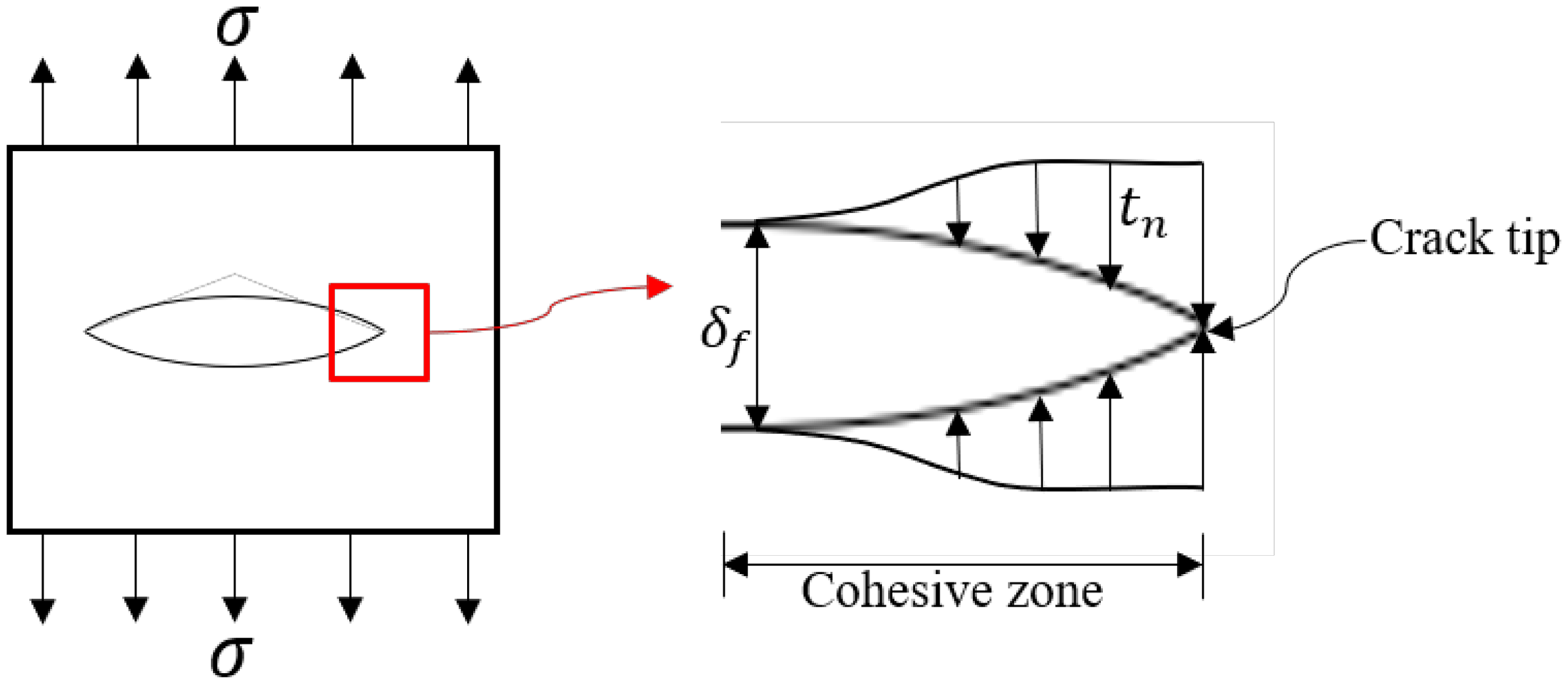
Illustration of the cohesive-zone model.

The bilinear and exponential curves are the two commonly used traction separation types in the FE model. This research uses the bilinear curves with the detailed traction separation of the CZM shown in Figure 2. The curves contain two parts. For the first part, the slope represents the effective elastic modulus (E_c) of a traction separation-based CZM and the effective elastic modulus is calculated as:

E_{c} = \frac{E_{a}}{T_{c}} \cdot T_{0}

(1)

where T_c is the original thickness of the cohesive layer, T₀ is the effective constitutive thickness, and E_a is the elastic modulus of the material. The effective elastic modulus affects the FEM convergence (Lin et al., 2017), and it should be designed to be a large number to ensure that CZM would only have a minor influence on the strain of the element before the damage occurs. Compared with traditional concrete, UHPC has a much smaller thickness of interfacial transition zone (ITZ), approximately 1–4 μm (Reda et al., 1999; Scheydt & Muller, 2012). Therefore, the initial thickness is set as 1 μm, and the effective constitutive thickness is set as unit length. As a result, the effective elastic modulus E_c is chosen to be 100 times the elastic modulus E_a.

Figure 2.

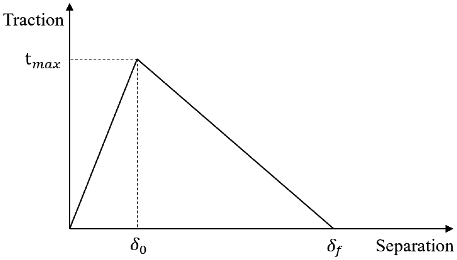
Illustration of traction separation curve.

For the bilinear traction separation curve, the stress components can be expressed as:

\begin{matrix} t_{n} = {\begin{matrix} (1 - D) \bar{t_{n}}, \bar{t_{n}} \geq 0 \\ \bar{t_{n}}, otherwise (no damage to compress stiffness) \end{matrix} \\ t_{s} = (1 - D) \bar{t_{s}} \\ t_{t} = (1 - D) \bar{t_{t}} \end{matrix}

(2)

where

\bar{t_{n}}

\bar{t_{s}}

, and

\bar{t_{t}}

are the stress components in the non-damaged status of the traction separation curve. Furthermore, D is the damage coefficient to describe the overall damage of the material. The expression of the damage coefficient is:

D = {\begin{matrix} 0, σ < f_{t} \\ \frac{δ_{m}^{f} (δ_{m}^{max} - δ_{m}^{0})}{δ_{m}^{max} (δ_{m}^{f} - δ_{m}^{0})}, δ_{m}^{max} < δ_{m}^{f} \\ 1, δ_{m}^{max} > δ_{m}^{f} \end{matrix}

(3)

where f_t is the tensile strength,

δ_{m}^{0}

is the displacement at the damage initiation,

δ_{m}^{f}

is the displacement at the complete failure, and

δ_{m}^{max}

refers to the maximum historical displacement. The damage evolution can be expressed as the combination of normal and shear stress components and the effective displacement

δ_{m}

, which contributes to describing the damage coefficient, can be defined as (Camanho & Dávila, 2002):

δ_{m} = \sqrt{⟨ δ_{n} ⟩^{2} + δ_{s}^{2} + δ_{t}^{2}}

(4)

where

δ_{n}

is the normal component of the relative displacement while

δ_{s}

and

δ_{t}

are the two tangential components of relative displacement of the element. For the second part of the traction separation curve, that is, the softening, when the stresses in the CZM reach the damage initialization criterion, the damage will occur, the damage coefficient will increase starting from 0, and the elastic modulus will start to decrease. When the damage coefficient reaches 1, the CZM will result in total failure and be removed from the FE model. Two adjacent elements will be separated, and the crack will be generated.

For this research, two kinds of CZMs are defined and used in the FE model. The first kind of the CZM ( ${CZM}_{matrix}$ ) is embedded between every two adjacent cement matrix elements to simulate the failure and crack propagation in the homogenized UHPC cement matrix. The second kind of CZM ( ${CZM}_{ITZ}$ ) is embedded between the fiber element and the cement matrix element to simulate the failure and crack propagation in ITZ. Therefore, all the parameters used in the traction separation curve should be determined for both kinds of CZM.

The effective elastic modulus of both kinds of CZM is set to be 100 times the elastic modulus. For the tangent direction, the effective elastic modulus is determined as $\sqrt{2}$ times the normal direction (Jun & Mio, 2019). The elastic modulus of the cement matrix and fibers were chosen from Qiao et al. (2016) as E_a = 31.3 GPa and E_f = 210 GPa. The Poisson ratio for the cement matrix and fibers are 0.2 and 0.3, respectively. The tensile strength of the homogenized UHPC cement matrix ( $T_{matrix}$ ) is determined by the analysis of the experimental data. The tensile strength of the ITZ ( $T_{ITZ}$ ) should be set as 0.35–0.70 times of the cement matrix CZM ( $T_{matrix}$ ) (Trawiński et al., 2016). In this study, the tensile strength ratio of the cement matrix to ITZ ( $T_{ITZ}$ / $T_{matrix}$ ) is approximately determined as 0.6, and the detailed tensile strength for the homogenized UHPC cement matrix ( $T_{matrix}$ ) and ITZ ( $T_{ITZ}$ ) are 9.6 MPa and 5.88 MPa, respectively (Qiao et al., 2016). The corresponding fracture energies are determined as 2.78 kJ/m² and 1.02 kJ/m², respectively (Wille & Naaman, 2010; Xu & Wille, 2015). The above CZM parameters are selected for the 0 cycle (i.e. the same situation as 7 days for curing age). Since the influence of curing age and the F–T cycles will be discussed, the CZM parameters group for each FE model should be determined.

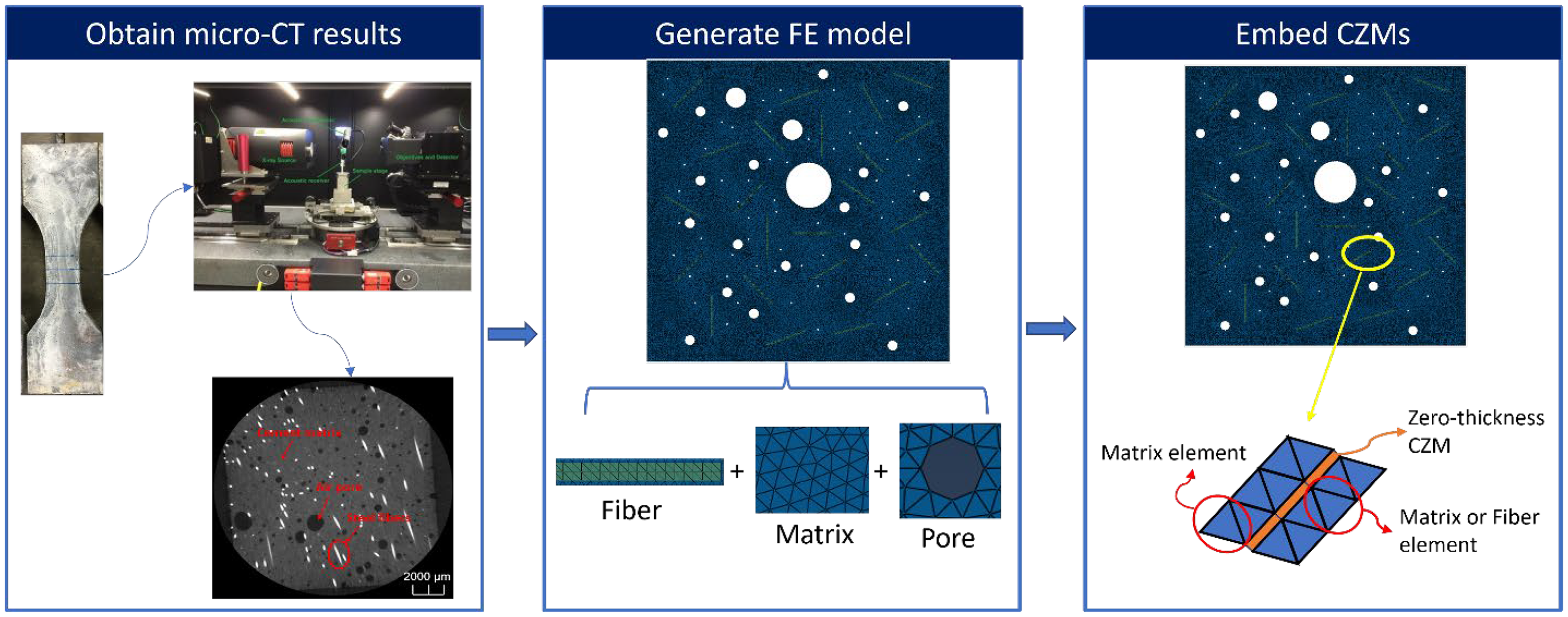
Considering the FE model for different curing ages (i.e. 7 days, 14 days, and 28 days), the elastic modulus of 14 days and 28 days samples are 104.56% and 113.67% of 7 days samples (Qiao et al., 2016). Therefore, for 14 days and 28 days, the effective elastic modulus for CZMs ( $E_{c, czm – matrix}$ , $E_{c, czm – ITZ}$ ) and homogenized matrix (E_a) is determined as 104.56% and 113.67% of the 7 days sample, respectively. The tensile strengths of 14 days and 28 days samples are 115% and 127% of the 7 days sample. The same CZM parameters as the 7 days (0 F–T cycles) will be used for 300 F–T cycles.

Multiscale modeling based on X-ray CT images

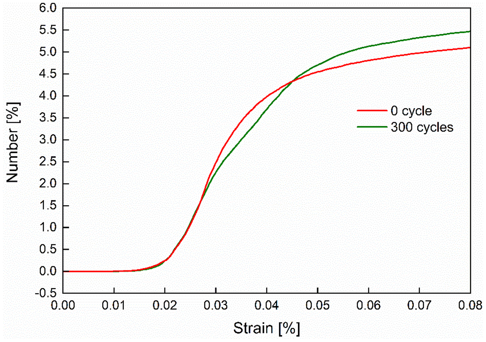
To accurately demonstrate the microstructure of UHPC specimens, the X-ray micro-CT technique is applied. Micro-CT scans are conducted with the ZEISS Xradia 410 Versa nano-CT modality (Luo et al., 2019), and the statistical information of pores and fibers in UHPC is shown in Table 1. Besides the porosity, pore distribution is determined. The pore sizes are divided into three ranges: 0.01–0.1 mm, 0.1–1 mm, and 1+ mm. Figure 3 shows the pore distribution. The scanned UHPC 300 F–T cycles specimen has larger pores and less fiber volume fraction than the 0-cycle specimen. The 0-cycle and 300-cycle specimens have a similar number of pores in the 0.01–0.1 mm range. NYCON-SF Type I steel fiber, which is 0.2 filament diameter and 13 mm length, provided by the Nycon Corporation is used in the scanned UHPC specimen. Steel fibers are added at a content of 2% of the UHPC volume. Compared with the 300 F–T cycles, the 0 cycle has a slightly higher volume fraction of fibers.

Figure 3.

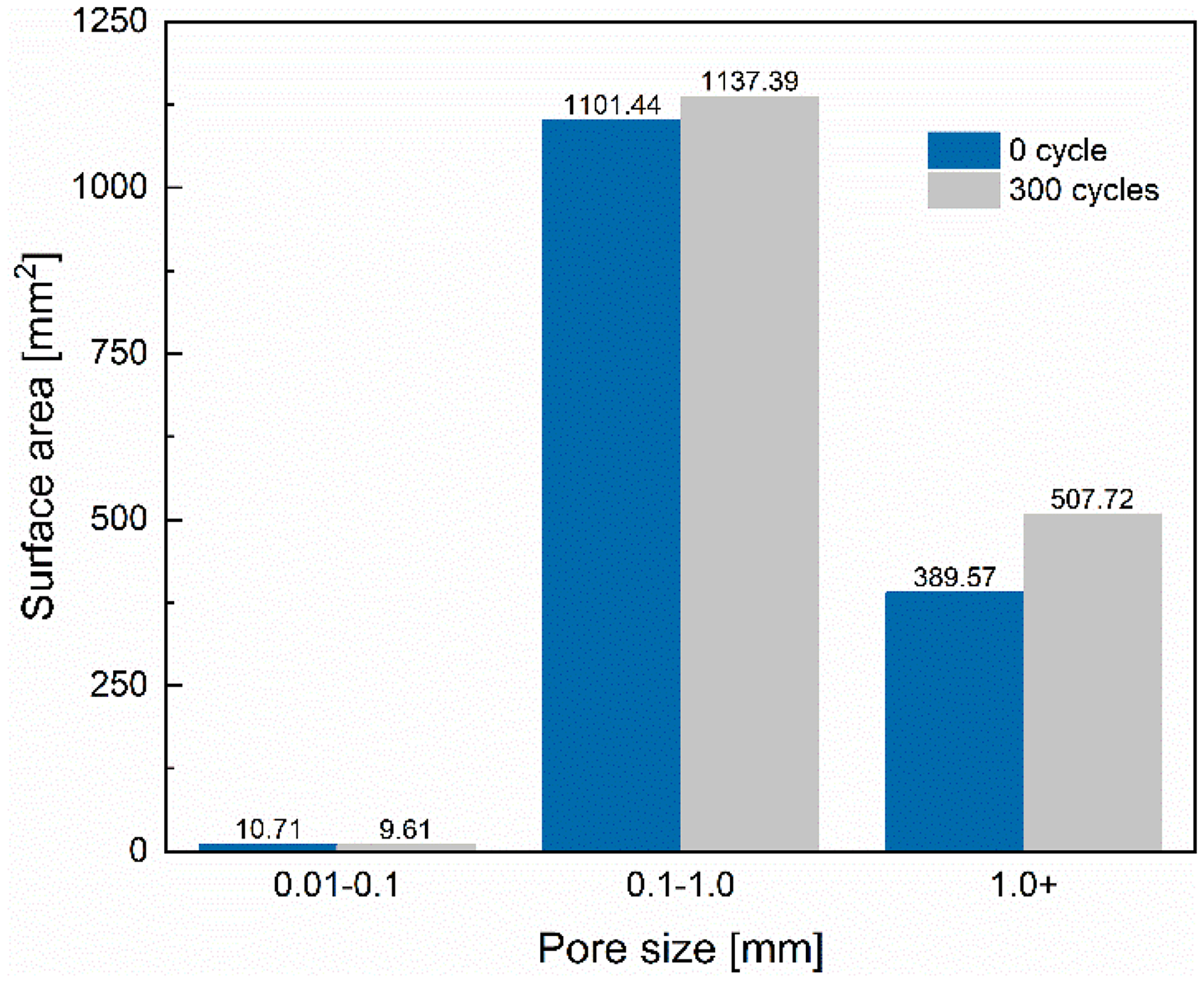
Pore distribution for different freeze–thaw (F–T) cycles.

Table 1.

Pore and fiber information in UHPC.

F-T cycles	Porosity (%)	Pore surface area, mm²	Volume fraction of fibers (%)
0	4.62	1502	2.11
300	6.73	1655	2.07

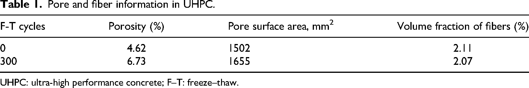
UHPC: ultra-high performance concrete; F–T: freeze–thaw.

When the micro-CT structure is obtained and the material properties parameters are finished, the representative volume element (RVE) can be further built using ABAQUS Version 6.14 (2014). Luo et al. (2019) addressed that when the size of RVE is >9 mm, the mean elastic modulus tends to be stable. For this research, the RVE size is selected as 14 mm rectangular. Two two-dimensional (2D) RVEs, one for 0 F–T cycle and one for 300 cycles, are built based on the micro-CT result. The detailed FE model mesh and zoom-in results are shown in Figure 4(a) and 4(b). As mentioned previously, the influence of curing age and F–T cycles will be discussed. It is important to clarify which FE model will be used for analyzing the effect of curing age as well as the effect of F–T cycles. To be specific, Figure 4(a) shows the mesh distribution for the first FE model used for the 0 F–T cycle and different curing ages while Figure 4(b) presents the FE model for 300 F–T cycles.

Figure 4.

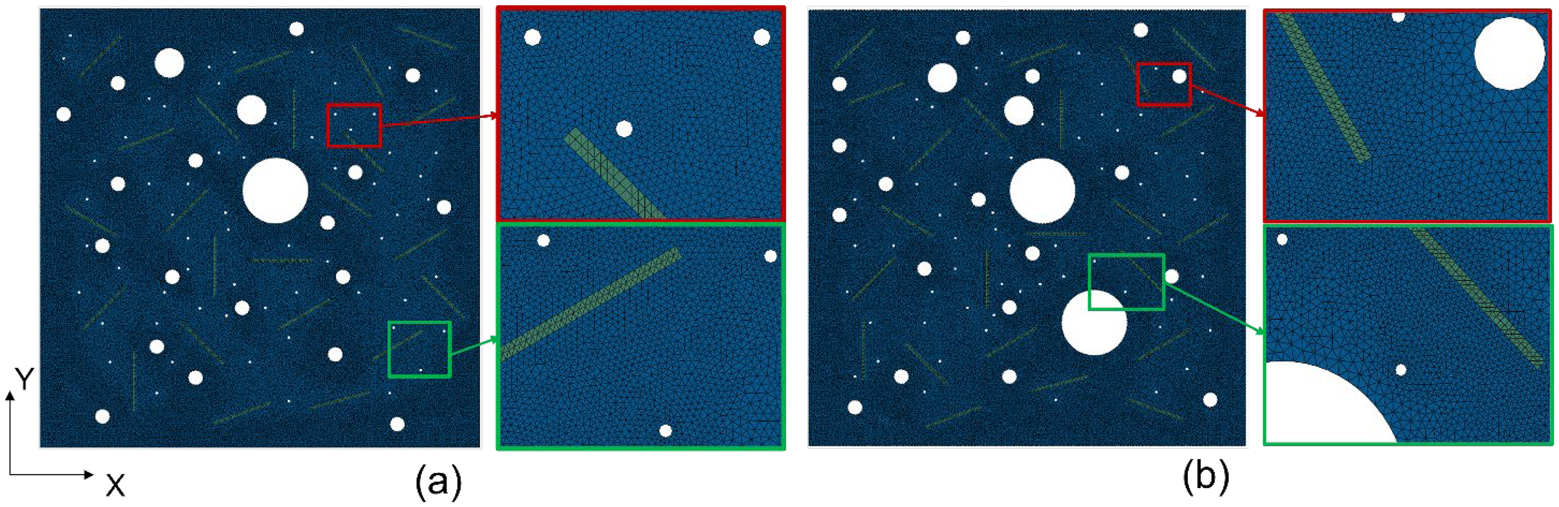
(A) FE mesh distribution (0 F–T cycle); (b) FE mesh distribution (300 F–T cycles).

The RVEs will not only include the fiber and matrix element but also include the cohesive-zone element to simulate the failure and crack propagation. Both the ${CZM}_{matrix}$ and ${CZM}_{ITZ}$ , which have been introduced in the “Cohesive-zone model and traction-–separation law” section, are set as the zero-thickness element and cannot be seen in Figure 4. The cohesive-zone element follows the discussed traction–separation law and when the traction increases between two adjacent elements, the cohesive-zone element can be extended. When the traction reaches maximum traction, the cohesive-zone element starts to degrade and finally be deleted. As a result, the microcrack will be formed and start to propagate.

This FE model contains 313,384 elements, including 185,909 cohesive elements and 127,475 triangle elements. Another FE model is built based on 300 F–T to analyze the influence of the F–T cycle. Figure 4(b) shows the mesh distribution of the second FE model. Precisely, 367,293 are used in this FE model, including 182,414 cohesive elements and 125,618 linear triangle elements. For the FE model in Figure 4, horizontal constraints are applied to the top boundaries ( $u_{x} = 0, r_{x} = r_{y} = 0$ ). The right boundary has no constraints. The bottom boundary is set to have vertical constrain ( $u_{x} = u_{y} = 0, r_{x} = r_{y} = 0$ ). A constant displacement loading is applied to the top side. A low loading rate (i.e. 0.001 in/s) is applied to ensure the FE model simulation loading is in a quasi-static state. When the boundary conditions are determined, the homogenization procedure will be addressed to obtain the stress and strain. Consider $σ_{22}$ and $ε_{22}$ are the volume average stress and strain, respectively. Since the RVE is a 2D element, the length in the Z direction will be considered as a unit length. The detailed expression of $σ_{22}$ and $ε_{22}$ is:

⟨ σ_{i j} ⟩ = \frac{1}{V_{r}} (\int_{V_{r}} σ_{i j}^{m} d V_{r} + \int_{V_{r}} σ_{i j}^{f} d V_{r})

(5)

⟨ ε_{i j} ⟩ = \frac{1}{V_{r}} (\int_{V_{r}} ε_{i j}^{m} d V_{r} + \int_{V_{r}} ε_{i j}^{f} d V_{r})

(6)

where

V_{r}

is the volume of the RVE,

σ_{i j}^{m}

and

σ_{i j}^{f}

are the stresses for the cement matrix and fiber, respectively, and

ε_{i j}^{m}

and

ε_{i j}^{f}

are the strains for the cement matrix and fiber, respectively.

The whole FE model modeling procedure can finally be addressed. First, the microstructural of UHPC is obtained from an X-ray CT scan. Based on the pore and fiber distribution, the 2D RVE model can be developed. Then, ${CZM}_{matrix}$ is inserted between each two adjacent cement matrix elements. ${CZM}_{ITZ}$ is inserted between each steel fiber element and the adjacent cement matrix elements. The detailed material properties should be determined from the above description. Figure 5 demonstrates the procedure of multiscale modeling procedure for RVE.

Figure 5.

Multiscale modeling procedure.

Results and discussion

When the multiscale modeling and homogenization procedure is done. The tensile strength result can be obtained. To analyze, the change of microstructure of RVE and the cohesive-zone elements parameters for matrix and ITZ will lead to which kinds of influence for the tensile strength, the parametric study should be addressed. That can be the reason why the influence of curing age and F–T cycles will be discussed. Considering the influence of curing age, the effective elastic modulus for the homogenized matrix (E_a) and CZMs ( $E_{c, czm - matrix}$ , $E_{c, czm - ITZ}$ ) will be changed. For the influence of F–T cycles, the microstructure of RVE will change. The detailed effect will be discussed in Sections “Influence of curing age” and “Influence of F–T cycles,” respectively.

Influence of curing age

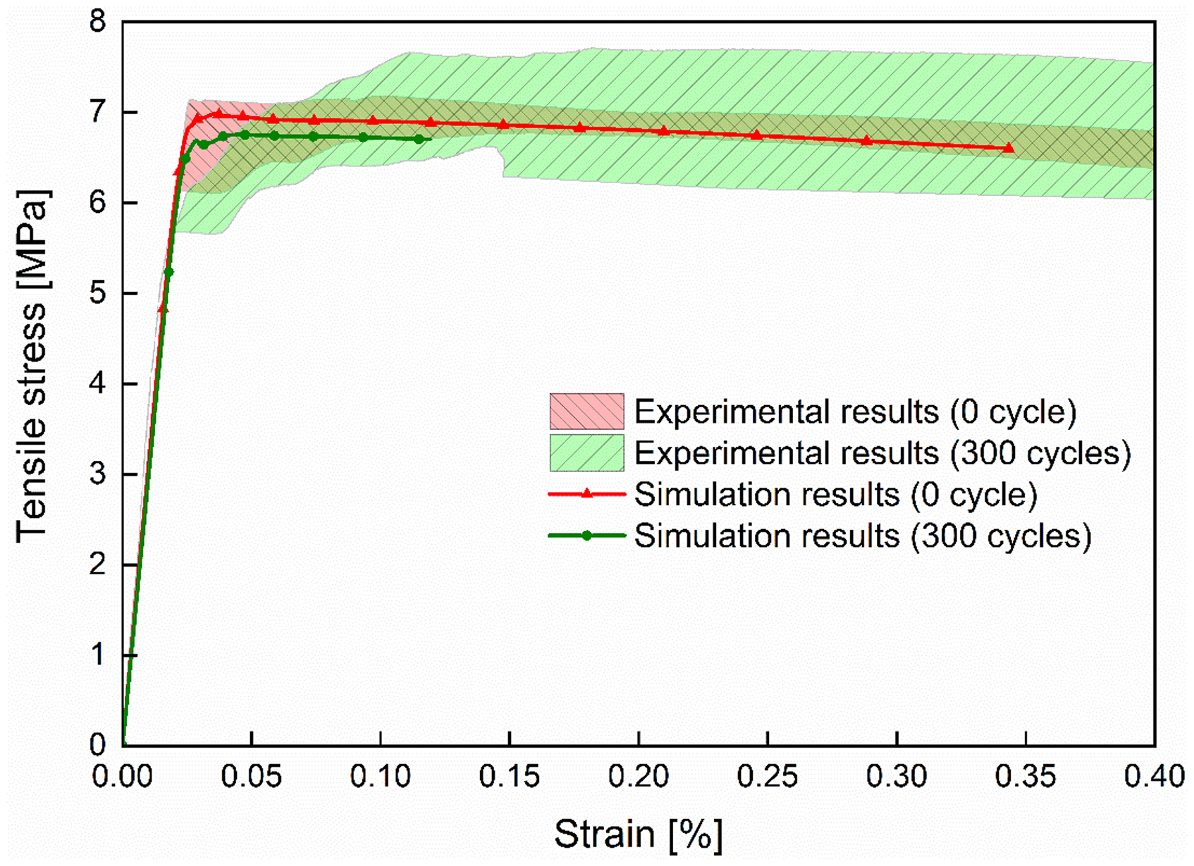
Simulation results considering different curing ages are discussed in this section. With the proposed FE model procedure, the simulation for three different curing ages (7 days, 14 days, and 28 days) is shown in Figure 6. For each case of curing ages, multiple experimental tests are conducted and the results are Qiao et al. (2016). In Figure 6, the range of the experimental tests for different curing ages is shown in different colors with sparse patterns. The shaded area for each pattern is obtained from the upper and lower limits of experimental tests. The FE model simulation results are shown in lines with different colors. The 28 curing days have the highest tensile stress for both experimental results (8.76 MPa) and simulation results (8.63 MPa). It is easy to observe that the simulation result for each curing age is within the area of the experimental result, which means the proposed FE models can obtain a good simulation result considering different curing ages.

Figure 6.

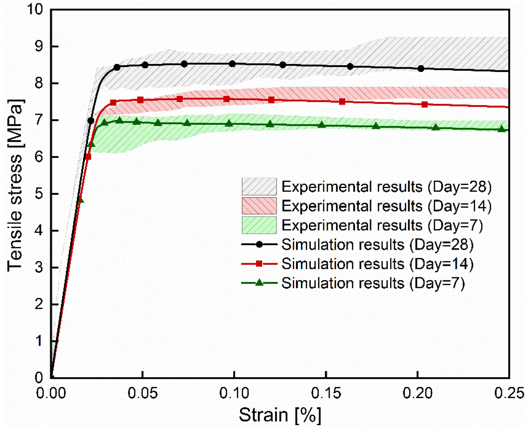
Finite-element simulation and comparison with experimental data for different curing ages.

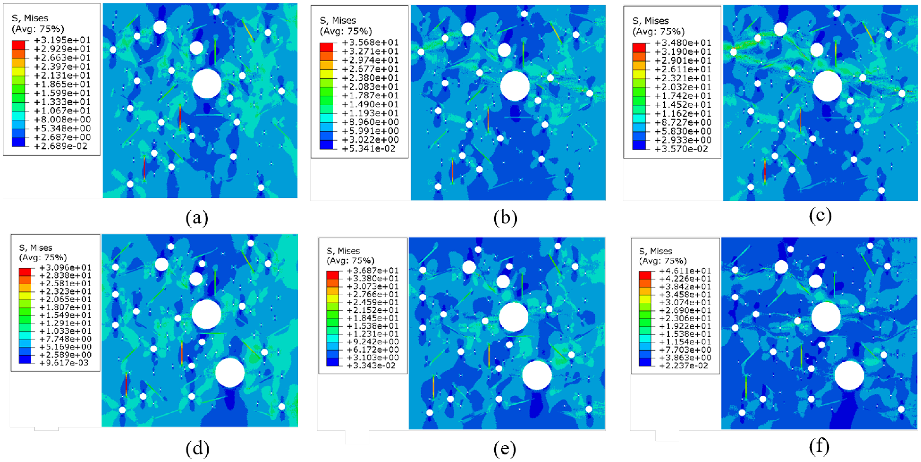
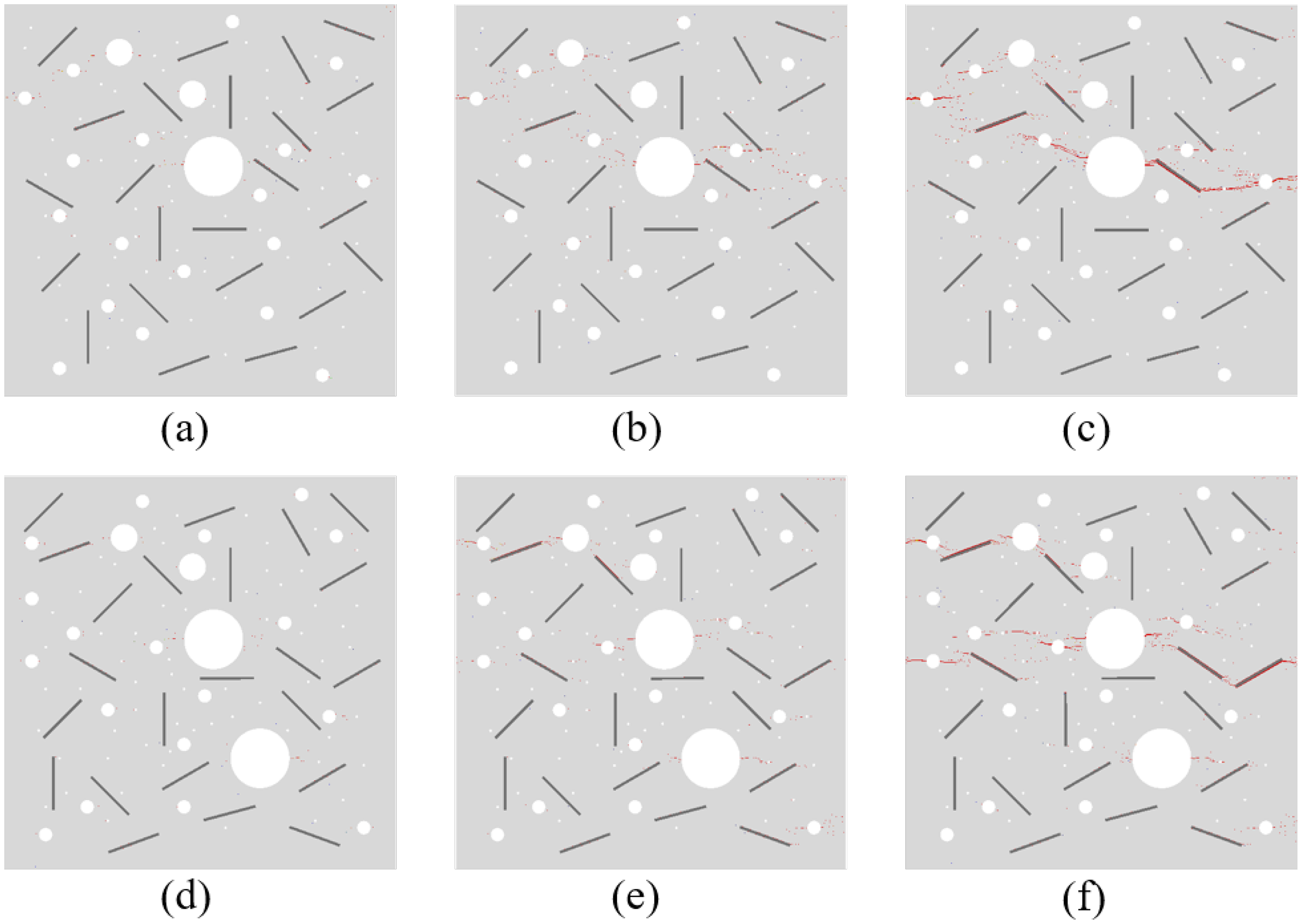
To capture the trend of tensile stress development across the entire simulation, three strain values (i.e. Strain = 0.029%, 0.042%, and 0.074%) are selected to split the curve into three parts based on Figure 6. Specifically, when the strain is <0.029%, the curve is almost a straight line. When strain is between 0.029% and 0.042%, the tensile strength is no longer linearly increased and starts to yield, and the strength starts to decrease. After Strain = 0.074%, the tensile strength begins to decrease linearly. Stiffness-degradation (SDEG) is one output parameter provided in the ABAQUS which can represent the overall scalar SDEG. Therefore, the SDEG can be used to demonstrate the crack information in the FE model. Figure 7 shows the SDEG status for the simulation of different curing ages, and the red lines in the figure represent the position where SDEG is >0.9. To clearly see the read lines, the edges between each element are selected to be invisible, and the cracks are scaled to be 10 times larger than the normal crack width. When strain equals 0.029%, cracks are already formed in the positions that have high stress. However, it is hard to see the cracks in Figure 7. Figure 8 is therefore provided to demonstrate the detailed simulation result of 7 curing days for the point where strain equals 0.029%. Three zoom-in sections are shown in the figure, which can more clearly display the crack propagation in the FE model. From the three zoom-in sections, it is easy to observe that the cracks are first formed and propagate from the horizontal direction of the pores and the edge of the fibers. When the strain equals 0.074%, the crack is already large enough to be observed in the full-scale FE model. The corresponding von Mises stress and stress in the vertical direction (S22) are further demonstrated in Figures 9 and 10. As observed in Figure 9, when the strain equals 0.029% for the 7-day sample (Figure 9(a)), the von Mises stress distribution is relatively uniform across the matrix with higher stress concentrations around the fibers and pores. As the strain increases to 0.042% (Figure 9(b)), the stress distribution becomes more uneven, with significant stress concentrations along crack paths and around fibers. When the strain reaches 0.074%, the stress concentrations are clearly visible along the major crack paths.

Figure 7.

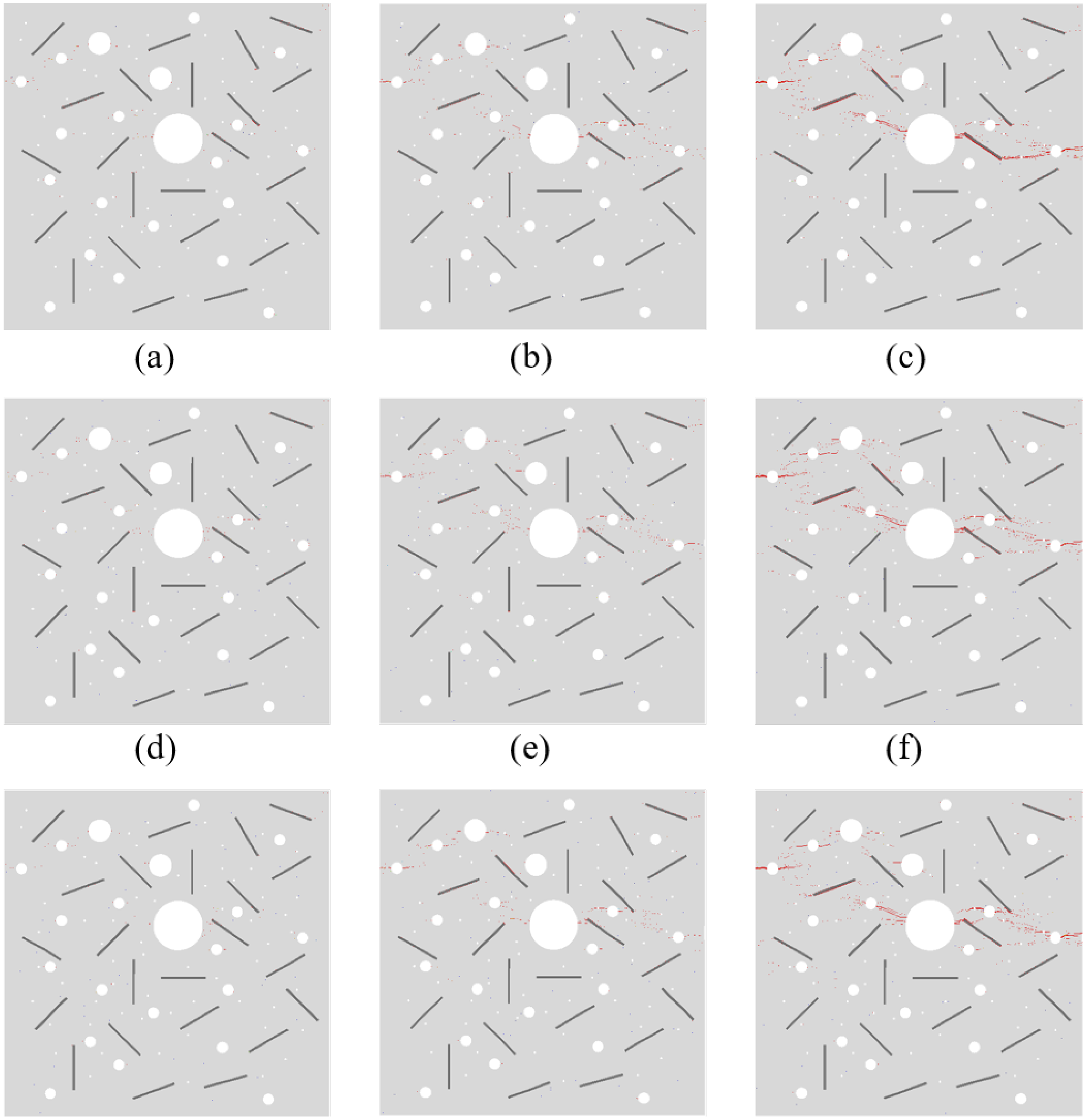
The stiffness-degradation (SDEG) plot. (a) Strain = 0.029% (7 days); (b) strain = 0.042% (7 days); (c) strain = 0.074%(7 days); (d) strain = 0.029% (14 days); (e) strain = 0.042%(14 days); (f) strain = 0.074%(14 days); (g) strain = 0.029% (28 days); (h) strain = 0.042%(28 days); and (i) strain = 0.074% (28 days).

Figure 8.

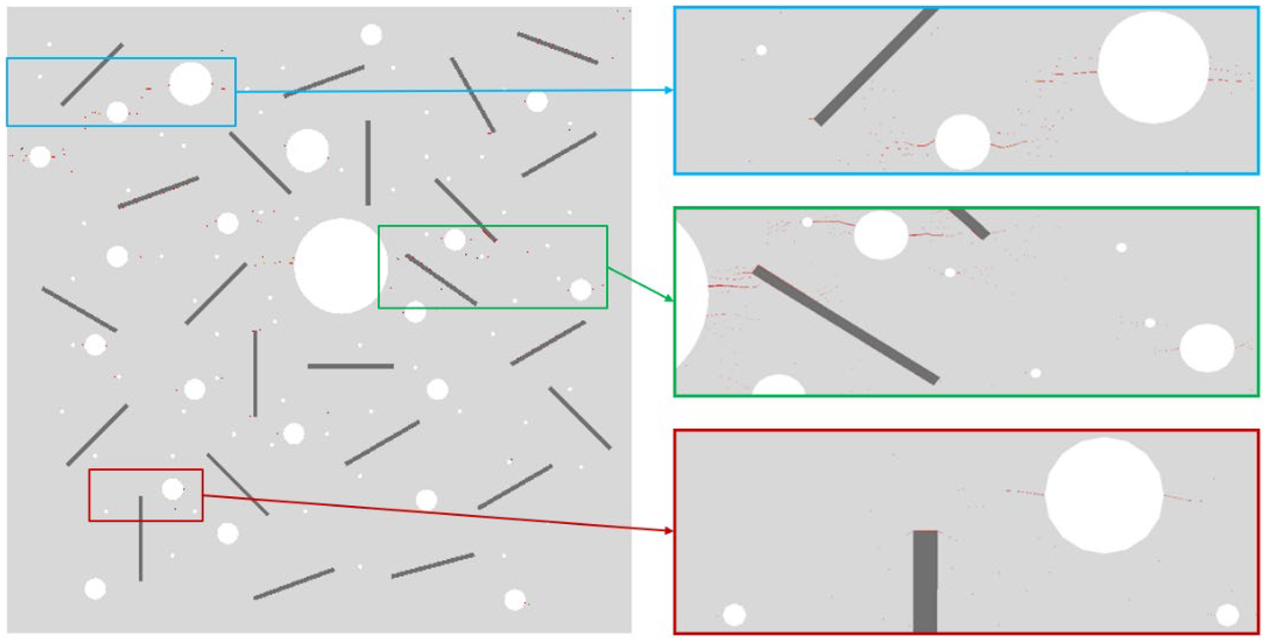
Detailed crack information for 7 days simulation.

Figure 9.

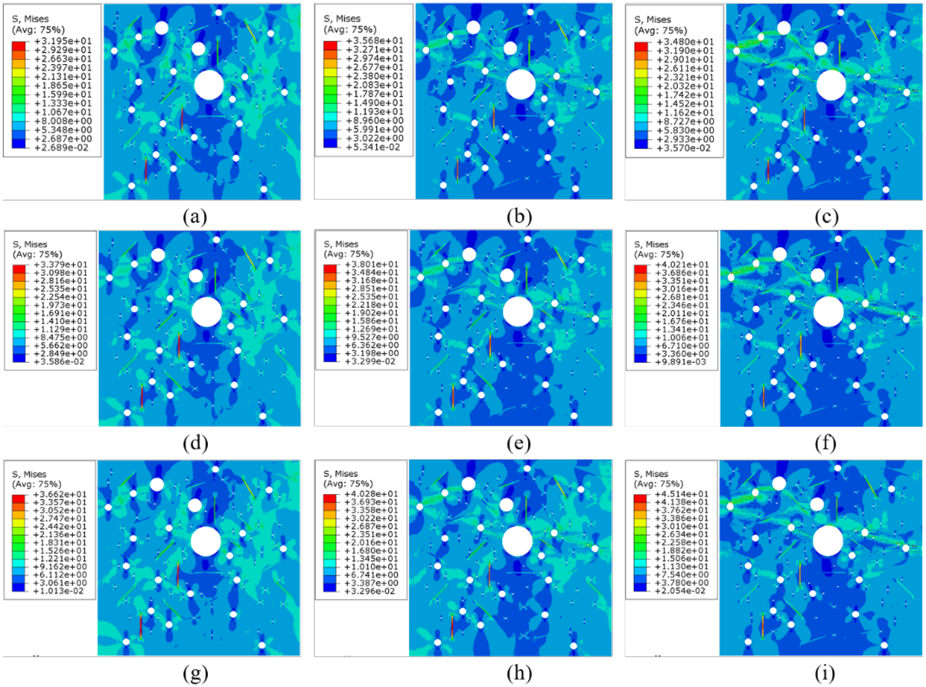
Illustration of von Mises stress. (a) Strain = 0.029% (7 days); (b) strain = 0.042% (7 days); (c) strain = 0.074% (7 days); (d) strain = 0.029% (14 days); (e) strain = 0.042% (14 days); (f) strain = 0.074% (14 days); (g) strain = 0.029% (28 days); (h) strain = 0.042% (28 days); and (i) strain = 0.074% (28 days).

Figure 10.

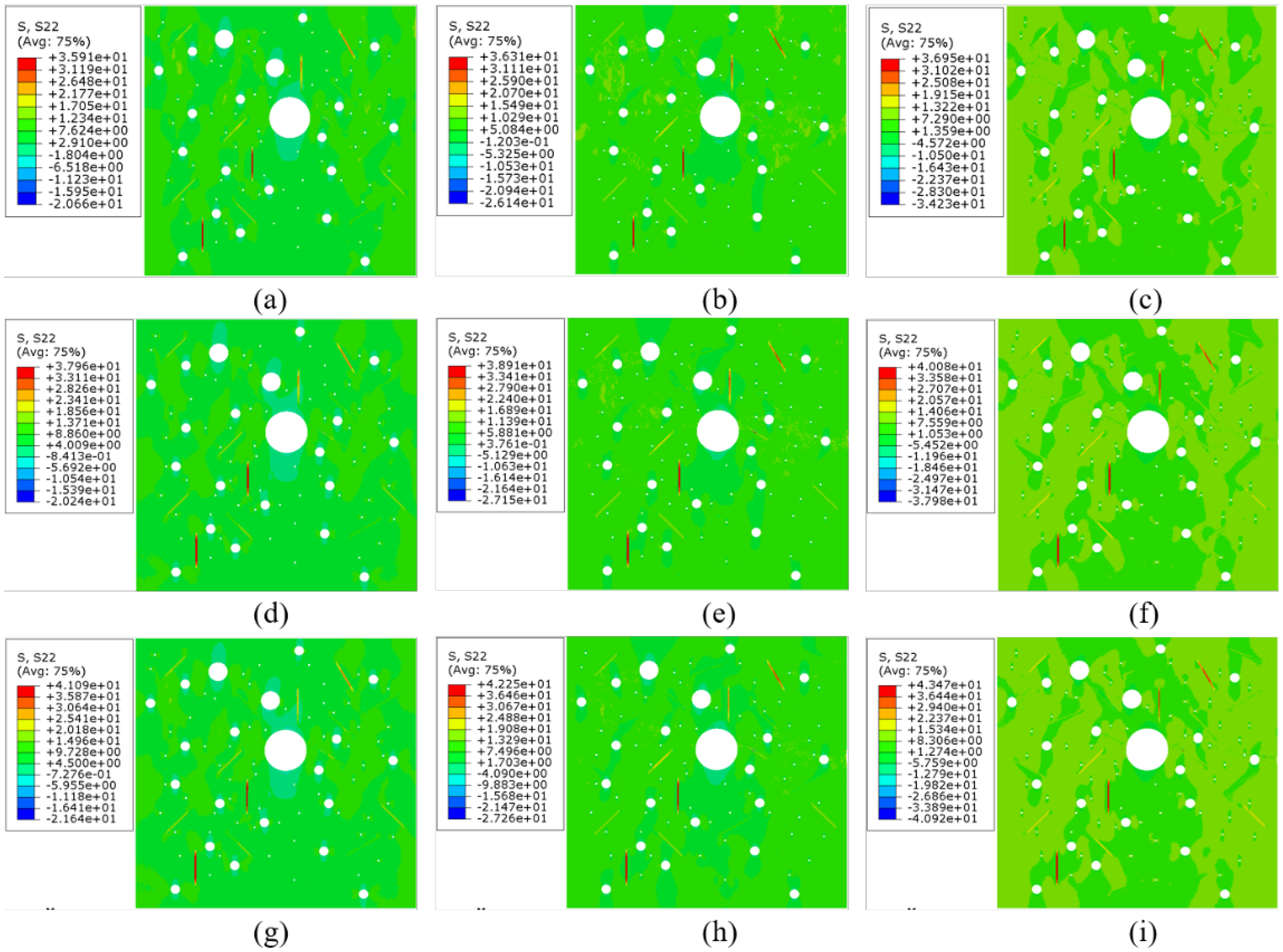
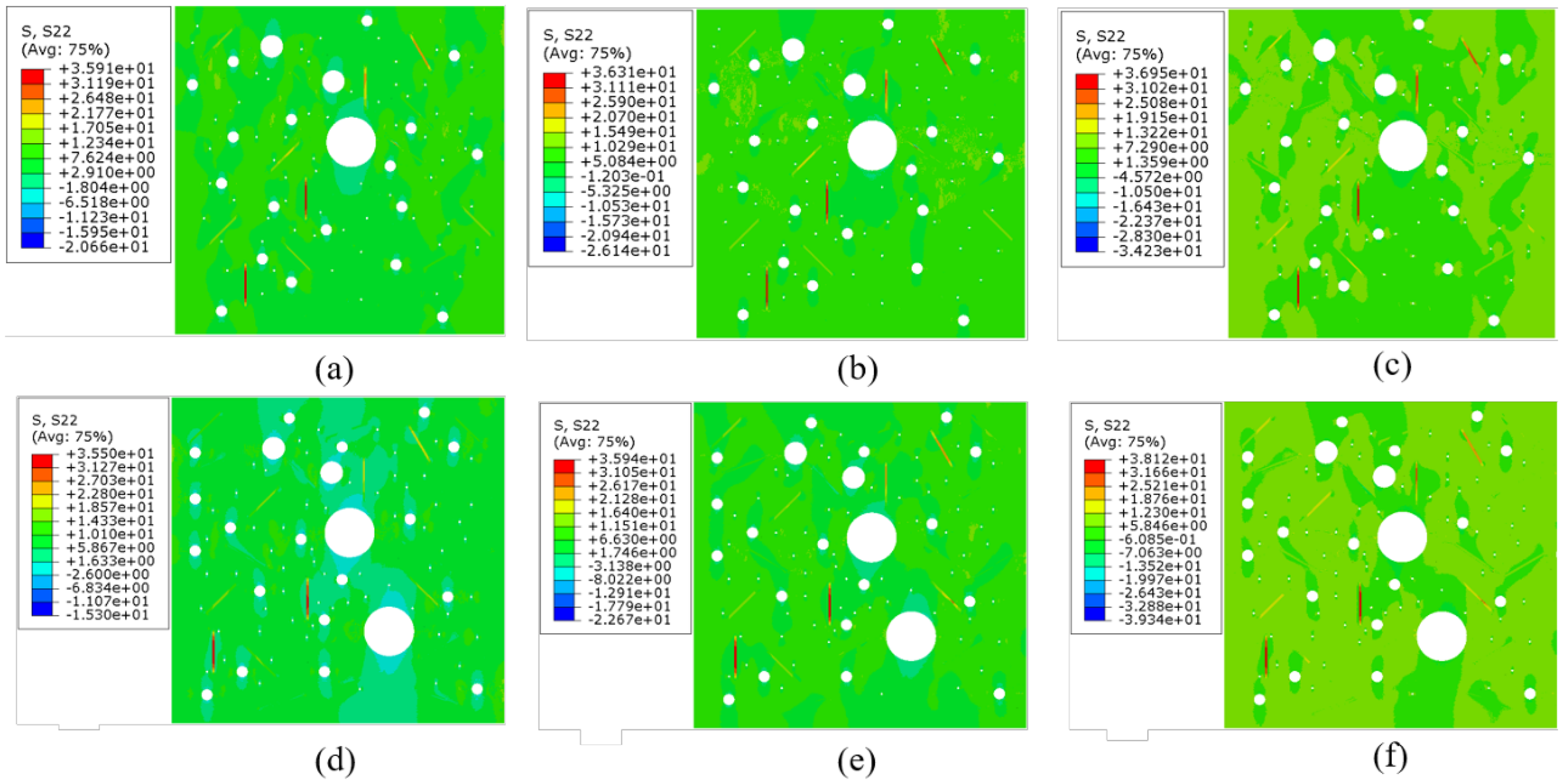
Illustration of stress in the vertical direction. (a) Strain = 0.029% (7 days); (b) strain = 0.042% (7 days); (c) strain = 0.074% (7 days); (d) strain = 0.029% (14 days); (e) strain = 0.042% (14 days); (f) strain = 0.074%(14 days); (g) strain = 0.029% (28 days); (h) strain = 0.042% (28 days); and (i) strain = 0.074% (28 days).

The above discussion and illustration indicate the proposed FE model matches the experimental results for 7-day curing ages. With the increment of curing ages, the material properties values are set up to increase, and FE models can still provide precise prediction results for the 14-day and 28-day curing ages compared with the experimental results.

Influence of F–T cycles

The FE model for the 0 cycle and 300 cycles are built based on the X-ray CT results in Table 1 and Figure 1. The simulation results are shown in Figure 11. The green area represents the experimental results (Qiao et al., 2016) for the 300 F–T cycles, and the corresponding simulation result is shown in the green line with the circle symbol. The average experimental peak tensile stress for 300 cycles is equal to 7.17 MPa, and the corresponding simulated peak tensile strength is equal to 6.75 MPa. Although the green line is not completely within the experimental result area, the peak tensile strength of the 300 cycles is still acceptable. The red area and red line represent the experimental results and simulation results for the 0 cycle, respectively. The averaged experimental peak tensile stress for the 0 cycle is equal to 7.04 MPa, and the corresponding simulated peak tensile strength is equal to 6.98 MPa. As a result, the proposed FE models can obtain a reliable tensile stress result considering the influence of F–T cycles. To clearly see the changes in the tensile stress, the first-order derivative of the simulation results is shown in Figure 12, representing the stress growth rates of 0 and 300 cycles, and they have a similar trend. The tensile stress growth rate can be roughly divided into three phases: strain = 0.00%–0.015%, strain = 0.15%–0.04%, and strain > 0.04%. For phase 1, the stress growth rate is a constant value. For phase 2, the stress growth rate decreases with fluctuations. For phase 3, the growth rate becomes a flat line and close to 0, which means the tensile strength is no longer increasing and begins to decrease gradually. Another observation is that the 300 cycles simulation has a smaller stress value in Phase 1 and has a larger negative value in Phase 2. As a result, 300 cycles simulations have a smaller peak tensile strength. The possible reason why the 300 cycles have a smaller peak tensile strength will be discussed during the rest part of this section.

Figure 11.

FE model simulation result for different F–T cycles.

Figure 12.

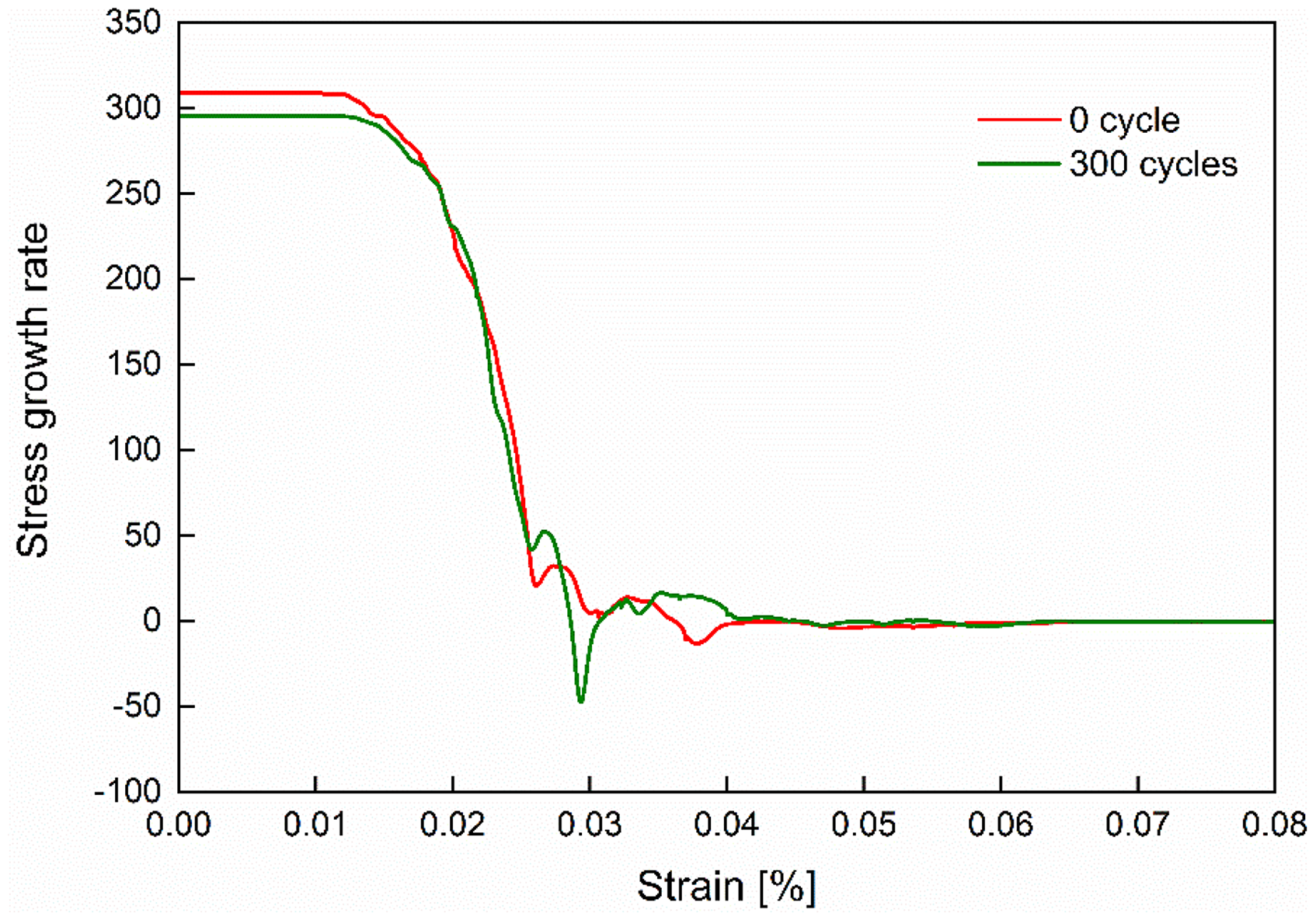
Tensile stress growth rate curve.

To analyze the simulation result for stress and crack information in detail, three strain values are selected: Strain = 0.029%, 0.042%, and 0.074%. The von Mises stress results for 0 cycle and 300 cycles are shown in Figure 13 and the stresses in the vertical direction (S22) are shown in Figure 14. Comparing the 0 and 300 cycles results, the 300 cycles simulation has a higher overall von Mises stress for each selected strain value. The von Mises stress and S22 distribution for 0 and 300 cycles are similar. High von Mises stress occurs at the fibers and along the crack path. When strain equals 0.029%, the peak S22 component for 0 and 300 cycles is close. When the strain increases to 0.042%, the 0 cycle has a higher peak S22 value. Three hundred cycles have a higher peak S22 value when the strain equals 0.074%.

Figure 13.

The illustration of von Mises stresses for different freeze–thaw (F–T) cycles. (a) Strain = 0.029% for 0 cycle; (b) strain = 0.042% for 0 cycle; (c) strain = 0.074% for 0 cycle; (d) strain = 0.029% for 300 cycles; (e) strain = 0.042% for 300 cycles; and (f) strain = 0.074% for 300 cycles.

Figure 14.

The illustration of stress in the vertical direction for different freeze–thaw (F–T) cycles. (a) Strain = 0.029% for 0 cycle; (b) strain = 0.042% for 0 cycle; (c) strain = 0.074% for 0 cycle; (d) strain = 0.029% for 300 cycles; (e) strain = 0.042% for 300 cycles; and (f) strain = 0.074% for 300 cycles.

Figure 15 shows the crack information for the mentioned sample strain points. The red lines in FE models represent the CZMs which have an SDEG value >0.9. To keep the same style of Figure 7, the edges between each element are selected to be invisible, and the cracks are scaled to be 10 times greater than the normal crack width as well. When strain equals 0.074%, cracks for the 0 cycle mainly propagate along the fiber edges and the largest pore while cracks for 300 cycles are more evenly distributed, and cracks propagate along with two large pores and the surrounding fibers.

Figure 15.

The SDEG plot for different F–T cycles. (a) Strain = 0.029% for 0 cycle; (b) strain = 0.042% for 0 cycle; (c) strain = 0.074% for 0 cycle; (d) strain = 0.029% for 300 cycles; (e) strain = 0.042% for 300 cycles; and (f) strain = 0.074% for 300 cycles.

After the SDEG distribution plots are obtained in Figure 15, a quantitative analysis of SDEG will be introduced. First, the number of cohesive elements that have an SDEG value >0.9, has been extracted in each simulation time step. Since 0 and 300 cycles, FEM has a different amount of cohesive element, the percentage of damaged cohesive element would be used to compare the damage of the 0 and 300 cycles. To be specific, the 0-cycle FE model has 185,909 cohesive elements while 300 cycles have 182,414 cohesive elements. The extracted number of damaged elements will divide the number of cohesive elements, and the results are shown in Figure 16. Figure 16 shows a quantitative analysis of the percentage of damaged cohesive elements (SDEG > 0.9) over the strain range for both 0 and 300 F–T cycles. This analysis offers insights into the damage evolution and crack propagation behavior under different F–T conditions. When the strain is <0.028%, 0 and 300 cycles have the same percentage of the damaged cohesive element, indicating that initial microcrack formation is not significantly influenced by the F–T cycles at this stage. When the strain is between 0.028% and 0.045%, the 0 cycle has a higher percentage of damaged cohesive elements compared to the 300 cycles. In other words, the initial microcrack in the 0 cycle propagates more rapidly than in the 300 cycles. However, the 300 cycles show a more gradual increase in the percentage of damaged elements and eventually exceed the 0 cycles case when strain is >0.045%.

Figure 16.

The percentage of the crack number.

The first-order derivative of the percentage of damaged cohesive elements can be described as the crack growth rate. The crack growth rates for 0 and 300 cycles are shown in Figures 17 and 18 with light purple and light blue, respectively. Since the original crack growth rate curves have a large fluctuating amplitude, it is hard to read the information based on the original crack growth rate curve. The Savitzky–Golay filter (Savitzky & Golay, 1964) is used for smoothing data points, and the smoothed curves are shown with dark purple and dark blue, respectively. In Figures 17 and 18, the stress growth rate, which is previously introduced in Figure 16, is also embedded in these figures. The crack growth rate curve can also be divided into three phases and matched with the previously introduced phases. As observed from Figure 17, at the initial Phase 1 stage, the stress growth rate remains relatively constant. The percentage of damaged cohesive elements is low, indicating minimal crack formation. This phase corresponds to the elastic behavior of the UHPC, where the material is primarily undergoing elastic deformation without significant damage. In Phase 2, the stress growth rate begins to decrease, accompanied by an increase in the percentage of damaged cohesive elements. This phase marks the start of the crack initiation and propagation. The UHPC starts to exhibit nonlinear behavior, and microcracks begin to form and grow, particularly around the fibers and pores. In Phase 3, the stress growth rate stabilizes at a low value, indicating the tensile strength is reaching its peak and beginning to decrease. The percentage of damaged cohesive elements continues to increase, showing continuous crack propagation. This phase represents the cracks in the material becoming widespread and eventually failure. Figure 18 shows the stress and crack growth curve for 300 F–T cycles. Similar to the 0 cycle, the stress growth rate is relatively constant, but it is lower than that of the 0 cycle. The percentage of damaged cohesive elements is also low. In Phase 2, the stress growth rate decreases more rapidly compared to the 0 cycle, with significant fluctuations. In Phase 3, the stress growth rate stabilizes at a negative value, indicating a decrease in tensile strength. The percentage of damaged cohesive elements is higher than in the 0 cycle. This phase highlights the impact of F–T cycles on the UHPC, resulting in more severe damage and reduced tensile strength.

Figure 17.

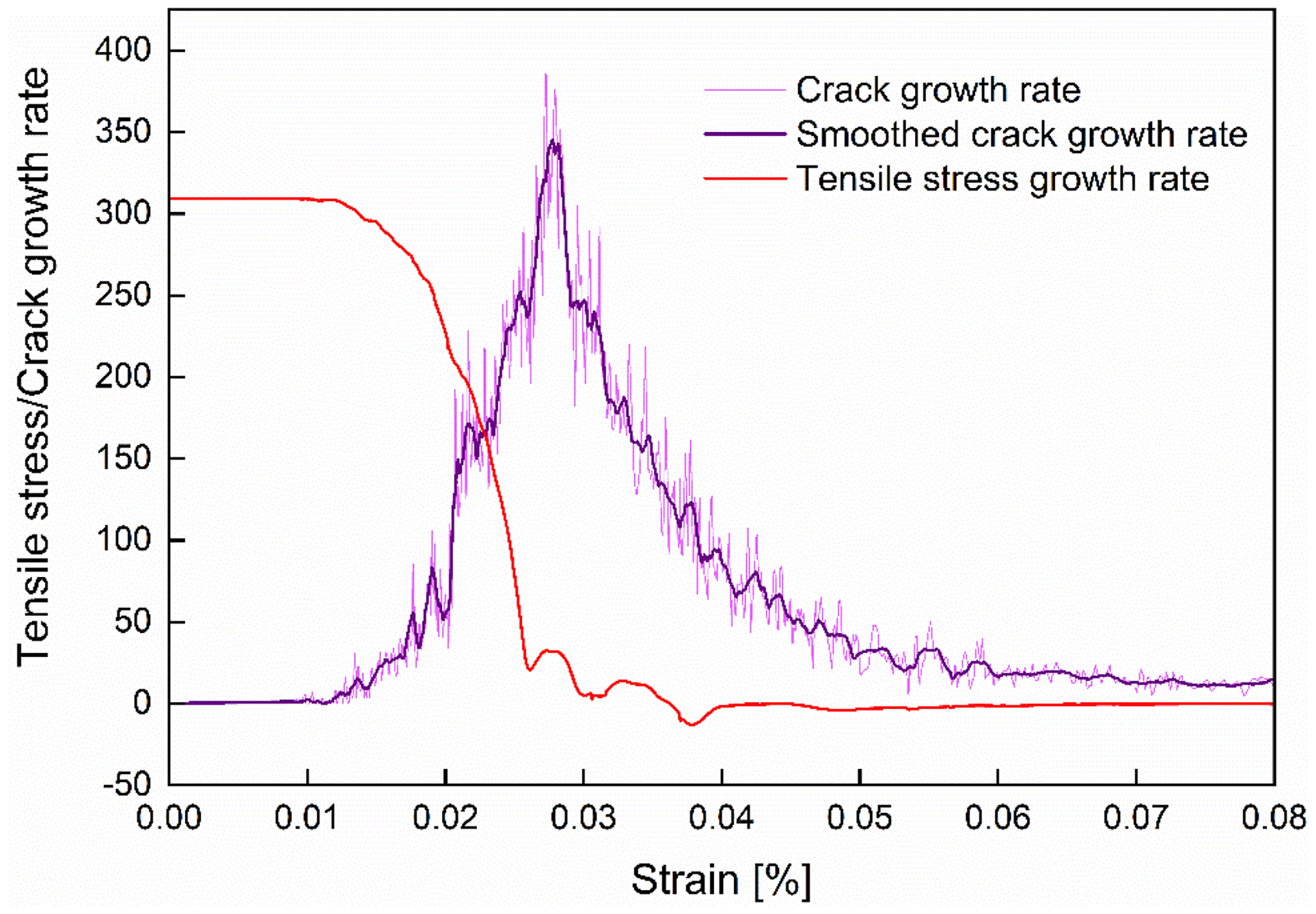
Stress and crack growth curve for 0 freeze–thaw (F–T) cycle.

Figure 18.

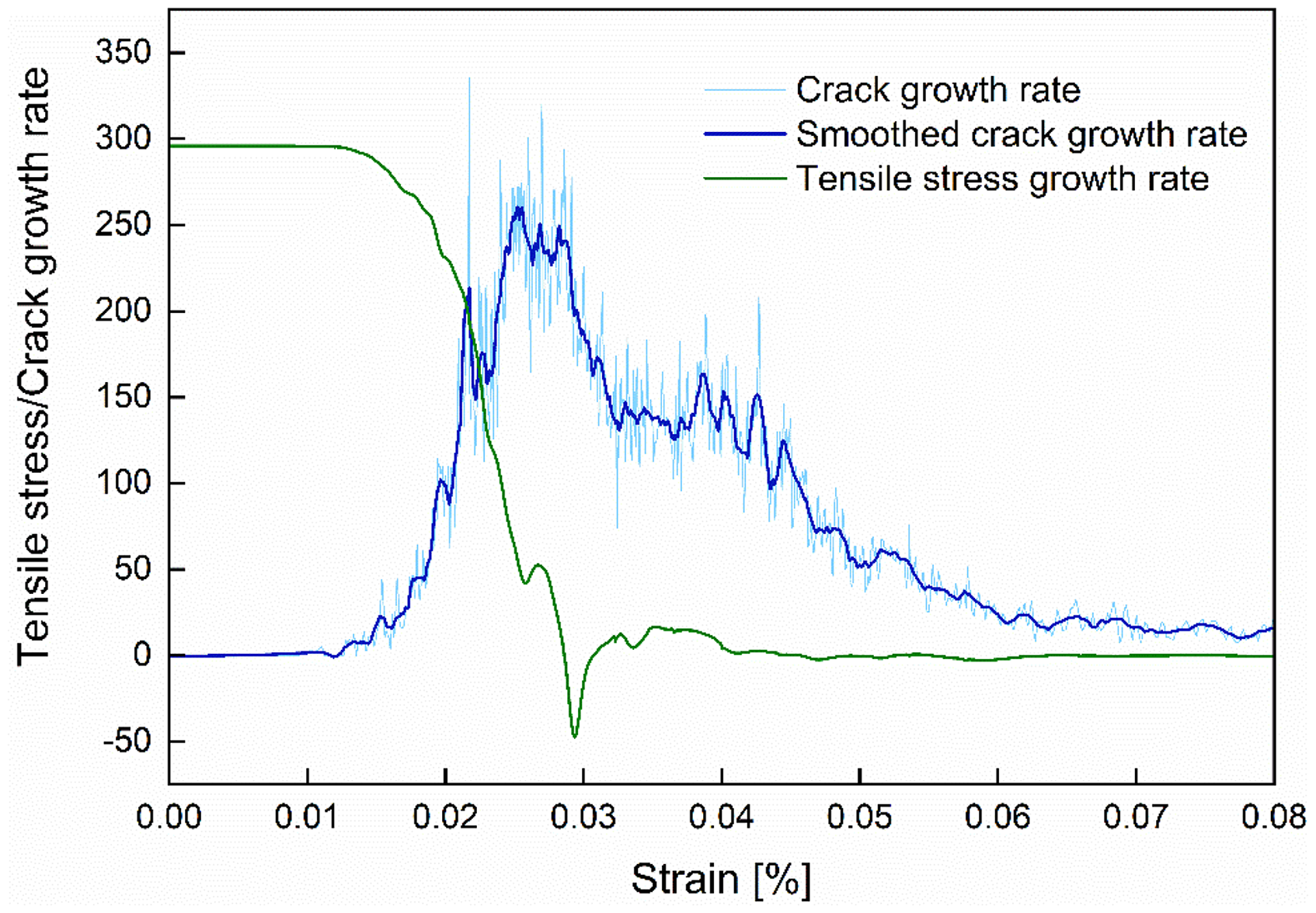
Stress and crack growth curve for 300 freeze–thaw (F–T) cycles.

Conclusions

This paper integrated the X-ray CT images and the CZM to construct the numerical FE models to simulate the tensile behavior of UHPC. Two kinds of cohesive-zone elements are used, the microstructural damage evolution is addressed, and the influence of curing age and F–T cycles are introduced. Considering the 7, 14, and 28 curing ages, the predicted simulation results show high consistency with the experimental direct tensile test. The FE model predicts a reasonable crack propagation path. As a result, the proposed FE modeling can be considered as a reliable approach to analyze the tensile behavior subject to different curing ages. Considering 0 and 300 F–T cycles, the proposed FE model gives a slightly smaller result than the direct tensile test result, which is still acceptable. Comparing the crack propagation paths of 0 and 300 cycles, the cracks of 300 cycles are more evenly distributed. The micro-scale analysis considering the ABAQUS output SDEG variable is further introduced to explain the damaged evolution of UHPC. The growth rate of simulated tensile strength and crack indicates that there is a high consistency between the failure of the cohesive-zone elements and tensile strength evolution. Therefore, the tensile strength behavior can be explained using the proposed CZM.

For the drawback of the current research, the proposed FE model is a 2D model. It is worth developing a three-dimensional (3D) FE model considering the X-ray CT images and compared with the proposed 2D model results. Also, the difference between the 0 and 300 cycles FE model is only limited to the difference in the pore and fiber fraction; more possible parameters that might influence the tensile strength behavior should be considered in the future. In addition, it would be interesting to apply the XFEM to analyze the tensile behavior of UHPC in the future.

Footnotes

Acknowledgments

The authors would like to thank Dr Dongxu Liu of the University of California, Irvine for providing UHPC CT images used in this study.

Declaration of conflicting interests

The authors declared no potential conflicts of interest with respect to the research, authorship, and/or publication of this article.

Funding

The authors disclosed receipt of the following financial support for the research, authorship, and/or publication of this article: This work was partially sponsored by the National Science Foundation under Grant No. CMMI-1229405.

References

Barenblatt

(1962) The mathematical theory of equilibrium cracks in brittle fracture. In: Advances in Applied Mechanics, Vol. 7. Elsevier, 55–129.

Brünig

Michalski

(2020) Numerical analysis of damage and failure behavior of concrete. International Journal of Damage Mechanics 29(4): 570–590.

Camanho

Dávila

(2002) Mixed-mode decohesion finite elements for the simulation of delamination in composite materials (No. NAS 1.15: 211737)

Campilho

Costa

Viana

, et al. (2017) Parameter identification in cohesive zone modelling. In: Strength Prediction of Adhesively-Bonded Joints. CRC Press, 161–208.

Dong

Qiao

, et al. (2018) Microstructural damage evolution and its effect on fracture behavior of concrete subjected to freeze-thaw cycles. International Journal of Damage Mechanics 27(8): 1272–1288.

Duarte

APC

Silvestre

de Brito

, et al. (2017) Numerical study of the compressive mechanical behaviour of rubberized concrete using the extended finite element method (XFEM). Composite Structures 179: 132–145.

Dugdale

(1960) Yielding of steel sheets containing slits. Journal of the Mechanics and Physics of Solids 8(2): 100–104.

Golewski

Sadowski

(2012) Numerical modelling crack propagation under mode II fracture in plain concretes containing siliceous fly-ash additive using XFEM method. Computational Materials Science 62: 75–78.

Hajar

Novarin

Servant

, et al. (2013) Innovative solution for strengthening orthotropic decks using UHPFRC: the Illzach bridge. In: Proceedings of International Symposium on Ultra-High Performance Fiber-Reinforced Concrete. October 1–3. Marseille, France.

10.

Hassan

AMT

Jones

Mahmud

(2012) Experimental test methods to determine the uniaxial tensile and compressive behaviour of ultra high performance fibre reinforced concrete (UHPFRC). Construction and Building Materials 37: 874–882.

11.

Jun

Mio

(2019) 8 – Time and temperature dependence of transverse tensile failure of unidirectional carbon fiber-reinforced polymer matrix composites. In: Woodhead Publishing Series in Composites Science and Engineering. Woodhead Publishing, 253–268.

12.

Kadhim

Semendary

Hammed

, et al. (2022) Numerical investigation of hybrid UHPC columns subject to lateral impact. Journal of Building Engineering 47: 103914.

13.

Larsen

Thorstensen

(2020) The influence of steel fibres on compressive and tensile strength of ultra high performance concrete: A review. Construction and Building Materials 256: 119459.

14.

Lin

Wang

Zeng

(2017) The role of cohesive zone properties on intergranular to transgranular fracture transition in polycrystalline solids. International Journal of Damage Mechanics 26(3): 379–394.

15.

Liu

Sun

(2006) Elastoplastic modeling of progressive interfacial debonding for particle-reinforced metal–matrix composites. Acta Mechanica 181: 1–17.

16.

Liu

Qiao

Sun

(2021) Characterization of microstructural damage evolution of freeze-thawed shotcrete by an integrative micro-CT and nanoindentation statistical approach. Cement and Concrete Composites 117: 103909.

17.

Luo

Liu

Qiao

, et al. (2019) Micro-CT-based micromechanics and numerical homogenization for effective elastic property of ultra-high performance concrete. International Journal of Damage Mechanics 29(1): 45–66.

18.

Mazzacane

Ricciotti

Teply

, et al. (2013) MUCEM: The builder's perspective. In: Proceedings of International Symposium on Ultra-High Performance Fiber-Reinforced Concrete. October 1–3.

Marseille, France.

3–16.

19.

Mechtcherine

Gram

Krenzer

, et al. (2014) Simulation of fresh concrete flow using discrete element method (DEM): theory and applications. Materials and Structures 47(4): 615–630.

20.

Moradi

Bagherieh

Esfahani

(2020) Constitutive modeling of steel fiber-reinforced concrete. International Journal of Damage Mechanics 29(3): 388–412.

21.

Moreillon

Menétrey

(2013) Rehabilitation and strengthening of existing RC structures with UHPFRC: various applications. In: Proceedings of International Symposium on Ultra-High Performance Fiber-Reinforced Concrete. October 1–3. Marseille, France.

22.

Nasrin

Ibrahim

(2018) Finite-element modeling of UHPC hybrid bridge deck connections. International Journal of Advanced Structural Engineering 10(3): 199–210.

23.

Park

Kim

Ryu

, et al. (2012) Tensile behavior of ultra high performance hybrid fiber reinforced concrete. Cement and Concrete Composites 34(2): 172–184.

24.

Park

Ahmed

Voyiadjis

(2022) A review of continuum damage and plasticity in concrete: Part I – theoretical framework. International Journal of Damage Mechanics 31(6): 901–954.

25.

Qiao

Allena

Zhou

(2016) Durability and smart condition assessment of ultra-high performance concrete in cold climates [Technical Report]. Available at: https://rosap.ntl.bts.gov/view/dot/32096.

26.

Raheem

AHA

Mahdy

Mashaly

(2019) Mechanical and fracture mechanics properties of ultra-high-performance concrete. Construction and Building Materials 213: 561–566.

27.

Rahman

McQuaker

(2016) Application of ultra high performance concrete in expediting the replacement and rehabilitation of highway bridges. July 18–20.

Des Moines, Iowa.

28.

Reda

Shrive

Gillott

(1999) Microstructural investigation of innovative UHPC. Cement Concrete Research 29(3): 323–329.

29.

Savitzky

Golay

MJJAc

(1964) Smoothing and differentiation of data by simplified least squares procedures. Analytical Chemistry 36(8): 1627–1639.

30.

Scheydt

Muller

(2012) Microstructure of ultra high performance concrete (UHPC) and its impact on durability. In: Proceedings of the 3rd International Symposium on UHPC and Nanotechnology for High Performance Construction Materials. March 7–9, Kassel, Germany.

31.

Shi

Xiao

Wang

, et al. (2015) A review on ultra high performance concrete: Part I. Raw materials and mixture design. Construction and Building Materials 101: 741–751.

32.

Shi

Kavoura

, et al. (2023) Uniaxial tensile response and tensile constitutive model of ultra-high performance concrete containing coarse aggregate (CA-UHPC). Cement and Concrete Composites 136: 104878.

33.

Tran

Donzé

F-V

Marin

(2011) A discrete element model of concrete under high triaxial loading. J Cement Concrete Composites 33(9): 936–948.

34.

Trawiński

Bobiński

Tejchman

(2016) Two-dimensional simulations of concrete fracture at aggregate level with cohesive elements based on X-ray μCT images. Engineering Fracture Mechanics 168: 204–226.

35.

Voyiadjis

Ahmed

Park

(2022) A review of continuum damage and plasticity in concrete: Part II – numerical framework. International Journal of Damage Mechanics 31(5): 762–794.

36.

Wang

(2006) Cohesive zone model of intermediate crack-induced debonding of FRP-plated concrete beam. International Journal of Solids Structures 43(21): 6630–6648.

37.

Wasantha

Bing

Yang

, et al. (2021) Numerical modelling of the crack-pore interaction and damage evolution behaviour of rocklike materials with pre-existing cracks and pores. International Journal of Damage Mechanics 30(5): 720–738.

38.

Wei

Zhu

Chen

, et al. (2023) Microstructure-based prediction of UHPC's tensile behavior considering the effects of interface bonding, matrix spalling and fiber distribution. Cement and Concrete Composites 139: 105015.

39.

Wille

Naaman

(2010) Fracture energy of UHPFRC under direct tensile loading. In: FraMCoS-7 International Conference. May 23–28. Jeju, Korea.

40.

Wille

(2015) Fracture energy of UHP-FRC under direct tensile loading applied at low strain rates. Composites Part B: Engineering 80: 116–125.

41.

Yin

Sun

(2005a) Elastic modeling of periodic composites with particle interactions. Philosophical Magazine Letters 85: 163–173.

42.

Yin

Sun

(2005b) Magnetoelasticity of chain-structured ferromagnetic composites. Applied Physics Letters 86: 261901.

43.

Jin

Liu

, et al. (2022) Mesoscopic finite element analysis on dynamic direct tensile failure of lightweight aggregate concrete and corresponding size effect. International Journal of Damage Mechanics 31(3): 403–425.

44.

Zhang

Xin

Correia

(2021) Fracture evaluation of ultra-high-performance fiber reinforced concrete (UHPFRC). Engineering Failure Analysis 120: 105076.

45.

Zhou

Qiao

(2019) Tensile behavior of ultra-high performance concrete: Analytical model and experimental validation. Construction and Building Materials 201: 842–851.

46.

Zhu

Wei

, et al. (2021) Statistical micromechanical damage model for SH-SFRC under tensile load considering the interfacial slip-softening and matrix spalling effects. International Journal of Damage Mechanics 30(9): 1423–1449.

Effect of microstructural damage evolution on tensile strength of ultra-high performance concrete: A multiscale numerical scheme

Abstract

Keywords

Introduction

Methodology

Cohesive-zone model and traction–separation law

Multiscale modeling based on X-ray CT images

Results and discussion

Influence of curing age

Influence of F–T cycles

Conclusions

Footnotes

Acknowledgments

Declaration of conflicting interests

Funding

References