Sage Journals: Discover world-class research

Abstract

The Group Actor-Partner Interdependence Model (GAPIM) conceptualizes group composition as a relational construct and provides methods for estimating the effects of compositional characteristics on outcomes of interest. This paper extends the GAPIM to a multilevel structural equation model framework, which expands the range of research questions the GAPIM might address, including those based on input-process-outcome models. Simulations, based on group size, number of groups, effect size, and compositional skewness, provide guidance for designing studies to maximize power to detect compositional effects. Discussion addresses composition in general, especially how “deep” characteristics become manifest and meaningful during interaction.

Keywords

group composition multilevel structural equation models interdependence

Group composition has long been of interest to scholars because of the assumption that who is in the group influences what the group does (Moreland & Levine, 1992). One way to think about composition is similarity. For example, consider a study in which age is the composition variable of interest. Some groups might consist of people in the same age bracket (e.g., 40–50), indicating high similarity among all members. Other groups might have a mix of people from different age brackets, in which case similarity is more nuanced; younger members are similar to each other but dissimilar from older members. The question is how to operationalize compositional similarity in groups and to assess how features of composition are related to the outcome of interest.

Kenny and Garcia (2012) introduced the Group Actor Partner Interdependence Model (GAPIM) to capture complex compositional characteristics of groups and their effects on process or outcomes. As discussed below, the GAPIM characterizes composition as a relational construct and decomposes composition into a set of discrete relationships among members of the group. However, the GAPIM in its original form is estimated via multilevel regression, which means its research applications are limited to models with one outcome or endogenous variable. As such, the GAPIM cannot readily analyze more complex hypotheses, for example, those based on the input-process-output model (IPO) in which process mediates the relationship between inputs and outputs; process and outputs are endogenous variables (Pavitt, 2014).¹ Thus, this article extends the GAPIM by situating it within a multilevel structural equation model (MSEM) framework, which broadens the types of research questions, including mediation, that the GAPIM might address. In addition, a set of simulations is provided to assess GAPIM performance across several design characteristics, including compositional configurations and degree of nonindependence in the outcome.

Overview

Before the GAPIM there was the actor-partner interdependence model (APIM) which, as the name implies, provides conceptual and statistical tools to evaluate whether and how interpersonal behavior and cognitions are associated (Cook & Kenny, 2005; Kenny & Ledermann, 2010; Kenny et al., 2006). It helps to think of the model as describing both an intrapersonal process (i.e., how one thinks or talks about X influences how one thinks or talks about Y) and an interpersonal one in which an interlocutor’s thoughts or comments about X influences self’s thoughts or comments about Y (Kenny, 2018). There are many examples in the interpersonal literature of these types of associations. For example, one’s satisfaction with a romantic relationship is related to his or her partner’s satisfaction (Proyer et al., 2019), and the same is true of commitment between partners (Tran & Simpson, 2009). It is the researcher’s responsibility to identify the plausible mechanisms by which influence occurs (e.g., why would one’s relational satisfaction be affected by his or her partner’s satisfaction?) and the ways in which satisfaction is conveyed or communicated that are meaningful for the research question of interest.

An important conceptual issue and modeling problem is whether participants are distinguishable on a characteristic of interest. In most cases, participants differ in a variety of ways and the choice of the distinguishing characteristic is (hopefully) based on theory. In some cases, it makes sense to distinguish dyad members based on gender, for example, heterosexual romantic couples, and in others gender is irrelevant (e.g., same-sex couples); partners are exchangeable on that characteristic.² The APIM for the distinguishable case is presented in Figure 1. Assuming a single predictor and outcome, actor scores are represented as $X$ and $Y$ and partner scores are indicated by a prime ( $X ’$ and $Y^{'}$ ). Thus, the actor’s score on the outcome, $Y$ , is influenced by her score on $X$ (the $a$ path) and her partner’s score on the predictor, $X^{'}$ (the $p^{'}$ path); the partner’s outcome, $Y^{'}$ , is affected by his score on $X^{'}$ and his partner’s score, $X$ . The double-headed arrow in Figure 1 indicates an association between the residual variances for both outcomes ( $Y$ and $Y^{'}$ ). As implied by the model, actor and partner paths are freely estimated and may vary. For example, in heterosexual married couples the effect of husbands’ level of commitment on wives’ satisfaction might differ from the effect of wives’ commitment on husbands’ satisfaction. Actor effects in the exchangeable case are constrained to be equal as are the partner effects because the assignment to actor and partner is arbitrary (e.g., either member of a sex-sex dyad can be designated as actor or partner).

Figure 1.

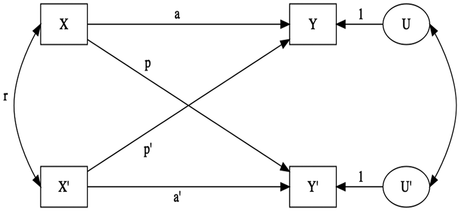
APIM for the distinguishable case.

Modeling Group Composition

The GAPIM extends features of the APIM to groups, most notably that group members are distinguishable on some relevant characteristic. Unlike the distinguishable case of the APIM, which evaluates outcome scores for each member of the dyad, the GAPIM uses only actors’ scores on the outcome (Kenny & Garcia, 2012).³ The predictor variable is also measured at the individual level but is transformed to represent several aspects of similarity. The predictor can be dichotomous or continuous but should be effect coded. (It seems counterintuitive to effect code a continuous variable. I will address the procedure for doing so below.) For example, assuming a binary gender variable, males might be arbitrarily coded with −1 and females +1. There are, of course, other examples of dichotomous composition variables; persons might be identified or experimentally manipulated into roles as experts and non-experts (e.g., Bottger, 1984). The same coding procedure applies and the researcher determines the assignment of codes to role. In the case of expertise, it might make sense to assign ones to experts because the interpretation, assuming a positive coefficient, is that scores on the outcome variable increase as expertise within the group increases.

The GAPIM consists of two main and two interaction effects. The first main effect is the actor effect, which is the association between a person’s score on the composition variable (which, as noted, is effect coded) and the outcome (which for current purposes is continuous). The others effect, the second main effect, is the association of the mean of the scores (still effect coded) on the composition variable of the other group members on the outcome.⁴ The others effect is interpreted as degree of similarity of one’s colleagues. For example, a lone male in a four-person group, assuming females have been coded 1, would have a score of one for the others effect, which indicates that the other three members are females. The scores for the three females in the group on the others effect would be $(1 + 1 - 1) / 3 = . 667$ ; that is, the other members consist primarily of females. Continuing with this example, the interpretation of the other affect, assuming a positive coefficient, is that the actor’s score on the outcome increases as the number of female partners increases or, put another way, as others’ gender becomes more similar.

The first of the two GAPIM interaction effects is actor similarity and addresses the degree to which the actor is similar to the others on the characteristic of interest. It is the product of the actor and others effect scores described above. The remaining interaction term, others’ similarity, is a dyadic measure that indicates the degree of similarity among pairs of one’s colleagues. It is operationalized as the mean of the interaction between (or product of) each pair of others’ scores on the characteristic of interest. Thus, for a four-person group with one male, the others’ similarity score for that male is $[(1 * 1) + (1 * 1) + (1 * 1)] / 3 = 1$ , and for each female in the group is $[(1 * - 1) + (1 * - 1) + (1 * 1)] / 3 = - . 33$ . For both interaction terms, a score of 1 indicates complete similarity and −1 complete dissimilarity. If actor similarity indicates the extent to which one is similar to the others on the characteristic of interest, others’ similarity captures the diversity at the dyadic level of the other members of the group.

Given the preceding, the GAPIM has five fixed-effects parameters, one for the intercept and the others for each of the effects described above. The GAPIM composition effects are measured at the within (i.e., individual) level but are technically mixed predictors, as they vary between and with groups. The model has two random effects, one for the intercept and the other the residual variance. The model, then, is expressed as:

y_{i k} = b_{0 k} + b_{1} X_{i k} + b_{2} X_{i k}^{'} + b_{3} I_{i k} + b_{4} {I^{'}}_{i k} + e_{i k}

(1)

Where $Y_{i k}$ is the score for Y on the outcome for person i in group k, $b_{0 k}$ is the intercept for group k, and $b_{1}$ , $b_{2}$ , $b_{3}$ , and $b_{4}$ are the actor effect, others effect, actor similarity, and others’ similarity, respectively. $X_{i k}$ is the score for the actor variable, $X_{i k}^{'}$ the score for the other effect variable, $I_{i k}$ the score for the actor similarity variable, and $I_{i k}^{'}$ the score for others’ similarity. The term $e_{i k}$ is the residual variance.

Intercepts ( $b_{0 k}$ ) for the outcome are treated as input at the second (between) level for each group. It is common to represent a given group’s intercept as the difference between the grand mean of the intercepts ( $γ_{00}$ ) and error, $u_{0 k}$ (Heck & Thomas, 2015):

b_{0 k} = γ_{00} + u_{0 k}

(2)

The distribution of the level 2 residuals has mean of 0 and a constant variance ( $μ$ ). Combining and substituting terms from equations (1) and (2) produces the following:

y_{i k} = γ_{00} + b_{1} X_{i k} + b_{2} X_{i k}^{'} + b_{3} I_{i k} + b_{4} I_{i k}^{'} + u_{0 k} + e_{i k}

(3)

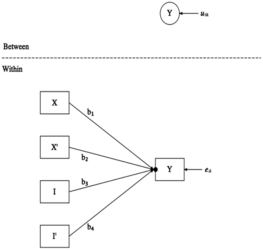
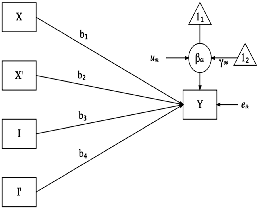
A graphical representation of the model is presented in Figure 2. The graph is based on Curran and Bauer’s (2007) recommendation for building path diagrams for multilevel regression models. Of interest is how the graph depicts the intercept random effect. As noted, $β_{0 k} = γ_{00} + u_{0 k}$ indicates deviation of group means ( $u_{0 k}$ ) from the grand mean ( $γ_{00}$ ). The intercept’s (the triangle with the label 1₁) path to the outcome has a circle superimposed on it that represents the latent group effect, which is influenced by both the grand mean ( $γ_{00}$ ) and its variance $u_{0 k}$ .

Figure 2.

The GAPIM as multilevel regression.

GAPIM Submodels

The model presented in equation (3) and Figure 2 is the complete or full model, as all terms are included without constraints. Many other options are possible depending on conceptual or analytic interests; only a subset is addressed here. The interested reader should consult Kenny and Garcia (2012) and the online appendix at http://davidakenny.net/doc/gapim_tech.pdf. The submodels are based on whether the main effects or interactions are estimated. The actor-only model assumes a significant actor effect but a nonsignificant partner effect ( $b_{1} \neq 0; b_{2} = 0$ ) whereas the partner-only model is the converse ( $b_{1} = 0; b_{2} \neq 0$ ). The group model contains significant and equal actor and partner effects ( $b_{1} = b_{2} \neq 0$ ) and the contrast model indicates actor and partner effects that are equal in magnitude but differ in sign ( $b_{1} - b_{2} = 0$ ). Of interest is the conceptual underpinnings of the contrast model, which implies that differences on the characteristic of interest drive outcomes. For example, recognizing one’s expertise as well as the lack of same in others might compel one to participate more frequently during discussion. One analytical option, described in detail below, is to compare model fit estimates to identify the best fitting submodel, though one might simply choose to work with the model that best matches the conceptual problem under consideration.

Estimating the GAPIM

The standard GAPIM is easily estimated with multilevel regression techniques, though applying constraints to some of the submodels presents considerable challenges. Here, we address how to estimate the unconditional (i.e., no predictors, used to evaluate the degree of nonindependence in the outcome), actor-only, partner-only, main effects, and full models using R’s lme4 package (Bates et al., 2015). (As demonstrated below, the submodel specification is much easier in MSEM.) The data are from the Arizona Trial Discussions Project (ATDP), a field experiment that assessed the effect of allowing jurors to discuss evidence among themselves prior to deliberation (Hannaford et al., 2000).⁵ In the experimental condition, judges’ instructions to the jury allowed discussion of the evidence; instructions in the contol condition prohibited such discussions. At the conclusion of the trial, jurors responded to a set of items regarding their experiences during the case as well as a few demographic questions.⁶ Data from 166 cases that made it to deliberation were used here—the remaining cases were settled prior to deliberation. Arizona civil trials use eight jurors and three alternates, all of whom hear the testimony. Thus, data from 1,360 jurors were available for analysis, average jury size = 8.19 (SD = 0.80). Seventy-nine participants did not provide gender information and were excluded from this analysis.

Categorical Predictor

For this demonstration, I focused on the item that asked participants “How much personal conflict was there on your jury?” Responses ranged from 1 (none) to 7 (a great deal). Gender is the composition variable (with females coded 1). The predictor, gender, must be converted to the three other GAPIM terms. The code for creating the GAPIM components in R and estimating the models in R’s lme4 is provided in Appendix A. Zero-order correlations, descriptive statistics, and intraclass correlations (ICC) are presented in Table 1. Note the very large ICCs for the others effect and others’ similarity and the moderate ICCs for the outcome and actor similarity.

Table 1.

Descriptive Statistics, Intraclass and Zero-Order Correlations for the Jury Data.

	M	SD	ICC	1	2	3	4	5
1. Actor effect	0.06	1.00	0.01	—
2. Others effect	0.06	0.40	0.86**	0.03	—
3. Actor similarity	0.02	0.41	0.20**	0.15**	0.03	—
4. Other’s similarity	0.02	0.26	0.73**	−0.02	0.16**	0.07*	—
5. Perceived conflict	6.08	1.43	0.17**	−0.03	−0.09**	−0.05	0.00	—

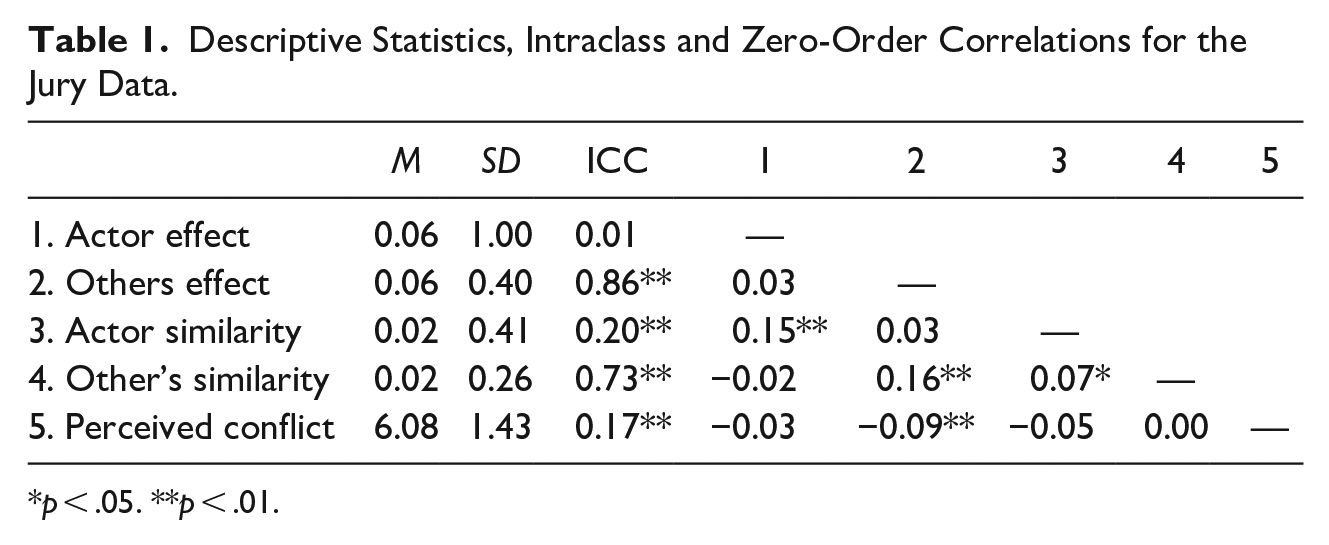
p < .05. **p < .01.

Table 2 contains estimates for the five models. The others effect is significant in all models in which it appears; none of the other GAPIM components are significant in any of the models. The negative coefficient indicates that perceived conflict decreases as the number of women in the group increases (or the number men in the group decreases). The actor similarity effect, although not significant, is interpreted as an increase in conflict the less similar one is to his or her colleagues. The ICC is the ratio of the group variance to residual variance, which for the full model is 0.35/1.69 = 0.17.

Table 2.

GAPIM Output, Categorial Predictor, Multilevel Regression.

Predictor	Unconditional	Actor only	Others only	Main effects	Full
Fixed effects
Intercept	6.08** (0.06)	6.08** (0.06)	6.10** (0.06)	6.10** (0.06)	6.10** (0.06)
Actor effect		−0.00 (0.04)		−0.03 (0.04)	−0.02 (0.04)
Others effect			−0.28* (0.13)	−0.31* (0.14)	−0.32* (0.14)
Actor similarity					−0.15 (0.11)
Others’ similarity					0.11 (0.20)
Random effects
Group variance	0.36	0.36	0.34	0.34	0.35
Residual	1.69	1.70	1.70	1.70	1.69
Deviance	4400.19	4400.18	4395.60	4395.07	4391.78

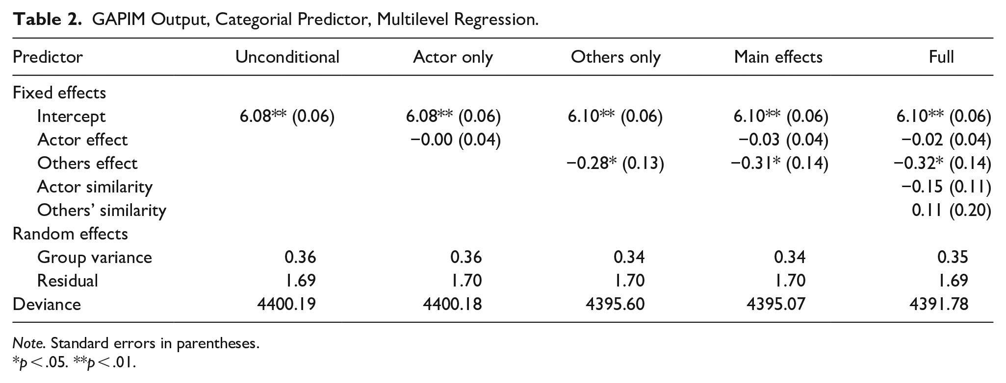
Note. Standard errors in parentheses.

p < .05. **p < .01.

Model comparison is often of interest. A common method of comparison is the chi-square difference test, which takes the difference of the deviance scores for each model. (Deviance is an indicator of model fit; lower scores indicate better fit.) The contrast in model deviance scores is distributed as a chi-square with degrees of freedom equal to the difference in model parameters. For example, the unconditional model has three parameters (fixed intercept, random intercept variance, and residual variance) and the others-only model has four (i.e., the same three as in the unconditional model plus the fixed term for the others effect). The deviance scores are 4400.19 and 4395.60 for the unconditional and others-only models, respectively. The others-only model provides a better fit, $χ^{2}$ (1) = 4.60, p = 0.03.⁷

Note that comparisons of the sort described above work only for models with different numbers of parameters. The actor-only and others-only models both have four parameters, which means the degrees of freedom for the chi-square test is zero; such comparisons are not allowed. In fact, many of the GAPIM submodels have the same degrees of freedom, which is one of the reasons why Kenny and Garcia (2012) suggest using the sample-size adjusted Bayesian information criterion (SABIC) to compare models, with smaller SABIC values indicating better fit. SABIC is computed as $D + q * l n ([N + 2] / 24)$ , where D is model deviance, q is the number of model parameters, ln is the natural logarithm, and N is the number of groups. Thus, SABIC for the actor-only model is 4400.18 + 4 × ln ([166 + 2]/24) = 4407.96 and that for the others-only model (substituting the proper deviance score) is 4403.38. By this metric, the others-only model provides a better fit to the data than does the actor-only model.

Continuous Predictor

In some cases, the composition variable of interest is not categorical. For example, the ATDP contained questions regarding age, education, and income. The response sets for each question are ranges, for example, 18 to 25 for age and $40,000 and $49,999 for income, though there are other ways for such data to be recorded. Here, education predicts level of difficulty in understanding evidence presented during the trial. The five ranges of education in the response set were less than 4 years of high school, high school graduate, some college, college graduate, and post-graduate work.⁸ The outcome, difficulty in understanding trial evidence, is measured on a scale of 1 (very difficult) to 7 (very easy). Due to missing data, 832 responses from participants in 156 juries were used in the analysis.

Descriptive statistics for the data are presented in Table 3 and MLM estimates for the unconditional, actor-only, others-only, main effects, and full models are in Table 4. Code for converting a continuous variable to effect codes is provided in Appendix A. The actor effect is significant and positive in all three models in which it appears, which indicates that trial evidence is easier to understand the higher one’s level of education. None of the remaining effects in any of the other models is significant. Although not presented here, one can perform model comparisons of the sort described above.

Table 3.

Descriptive Statistics, Intraclass and Zero-Order Correlations for the Jury Data.

	M	SD	ICC	1	2	3	4	5
1. Actor effect	−0.01	0.82	0.00	—
2. Others effect	−0.01	0.34	0.45**	−0.33**	—
3. Actor similarity	−0.09	0.31	0.08**	−0.03	0.04	—
4. Other’s similarity	−0.08	0.28	0.08**	0.06	−0.05	−0.42**	—
5. Difficulty understanding	5.40	1.37	.18**	0.07*	−0.01	−0.02	0.02	—

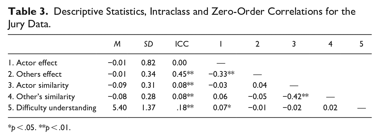
p < .05. **p < .01.

Table 4.

GAPIM Output, Continuous Predictor, Multilevel Regression.

Predictor	Unconditional	Actor only	Others only	Main effects	Full
Fixed effects
Intercept	5.40** (0.06)	5.39** (0.06)	5.39** (0.06)	5.39** (0.06)	5.39** (0.07)
Actor effect		0.12* (0.05)		0.14* (0.07)	0.13* (0.06)
Others effect			−0.13 (0.15)	0.09 (0.18)	0.07 (0.19)
Actor similarity					−0.22 (0.20)
Others’ similarity					−0.01 (0.21)
Random effects
Group variance	0.33	0.33	0.34	0.33	0.31
Residual	1.53	1.54	1.55	1.54	1.53
Deviance	2922.89	2863.21	2867.37	2862.98	2824.55

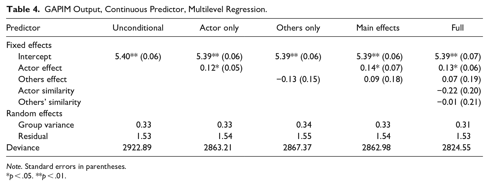
Note. Standard errors in parentheses.

p < .05. **p < .01.

Extending the GAPIM: An SEM Approach

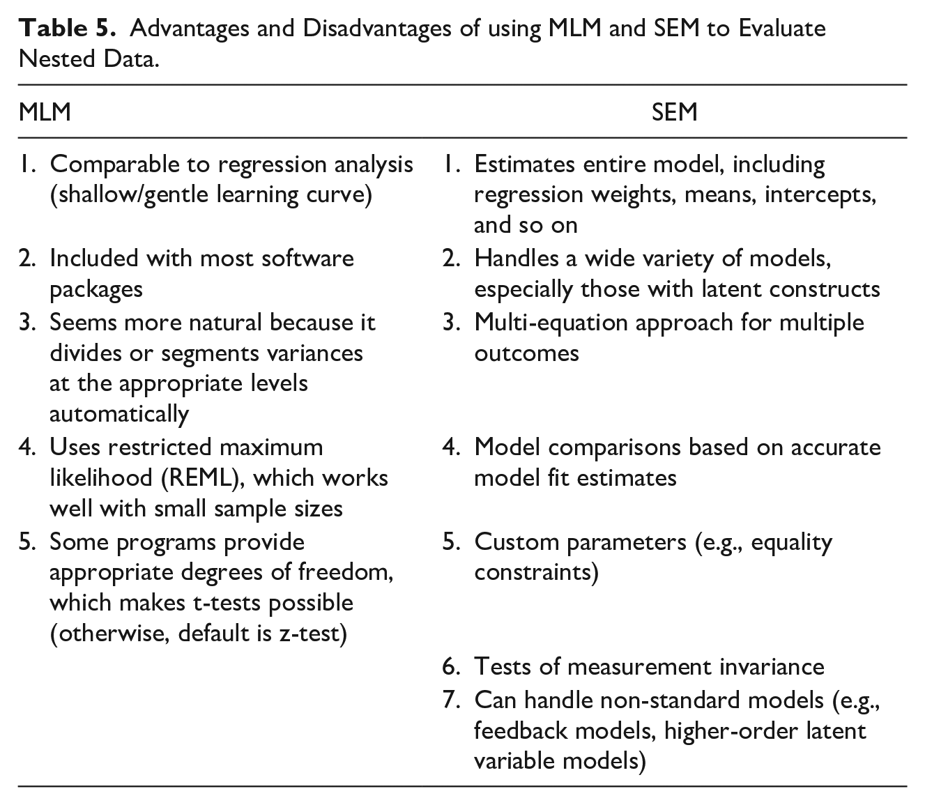
Regression models are really just path models, but because there is only one outcome and all effects are direct (including moderators) it is common and more convenient to use linear models to generate estimates. And in the case of the GAPIM, in which data are nested, mixed model estimation is the preferred option which, among other things, allows the investigation of random intercepts and slopes (i.e., that the outcome mean and regression coefficients might vary across groups). But rethinking the GAPIM as a multilevel path model reveals a set of possibilities that extend the model’s application. Ledermann and Kenny (2017) compared and contrasted traditional MLM and SEM approaches to modeling the APIM, though their argument applies equally well to using MSEM to evaluate multilevel regression models. See Table 5 for a list of relevant advantages for each approach. The gist is that MSEM is much more flexible than traditional MLM approaches. One important point in favor of the MLM is that it is familiar to most researchers, but familiarity does not necessarily make for appropriate or adequate analyses. Perhaps the most important point in favor of MSEM is the flexibility to include multiple outcome variables and indirect effects (Preacher et al., 2010), as well as latent constructs (Marsh et al., 2009). Imposing equality constraints on estimates is also quite easily done within the MSEM framework, which is an advantage for GAPIM submodel estimation.

Table 5.

Advantages and Disadvantages of using MLM and SEM to Evaluate Nested Data.

MLM	SEM
1. Comparable to regression analysis (shallow/gentle learning curve)	1. Estimates entire model, including regression weights, means, intercepts, and so on
2. Included with most software packages	2. Handles a wide variety of models, especially those with latent constructs
3. Seems more natural because it divides or segments variances at the appropriate levels automatically	3. Multi-equation approach for multiple outcomes
4. Uses restricted maximum likelihood (REML), which works well with small sample sizes	4. Model comparisons based on accurate model fit estimates
5. Some programs provide appropriate degrees of freedom, which makes t-tests possible (otherwise, default is z-test)	5. Custom parameters (e.g., equality constraints)
	6. Tests of measurement invariance
	7. Can handle non-standard models (e.g., feedback models, higher-order latent variable models)

MSEM allows specification of structures at both levels of analysis (assuming two levels; there can be more). There are several ways to graph MSEMs (Hox et al., 2018; Preacher et al., 2010; Rabe-Hesketh et al., 2004), though the Mplus (Muthén & Muthén, 1998–2017) approach is used here. The full GAPIM is depicted as an MSEM in Figure 3. Note that the within part of the model contains the regression structure from Figure 2. Mplus convention is to represent random intercepts as solid dots on the endogenous variable and to have the arrows from the predictors point to the dot. (Though not shown here, random slopes have a dot on the midpoint of the arrow for path of interest.) All variables in the within section of the graph are in rectangles or squares because they are observed (i.e., manifest), whereas variables in the between section are represented as circles or ellipses;⁹ variables at the between level are the unobserved or latent means of the manifest variables in the within section.¹⁰ The error terms at each level are also unobserved, though convention is to use labeled arrows that point to the variable, not nodes.¹¹ The ratio of the between-level variance to total variance (i.e., the sum of between and within variance) is the ICC.

Figure 3.

GAPIM represented as MSEM.

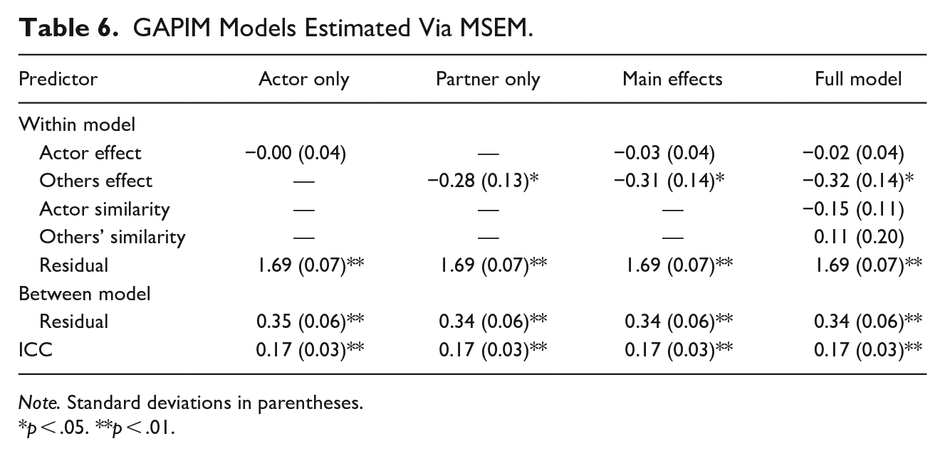
As noted, estimation of most GAPIM submodels using multilevel regression is quite challenging but doing so within the context of MSEM is a fairly simple matter. Table 6 presents model estimates for data from the ATDP in which perceived conflict is the outcome. The first model includes only the actor effect (i.e., all remaining effects constrained to 0), the second the others-only model, the third the main effects (actor and others effects estimated–both interactions constrained to 0) and the full model (i.e., all main and interaction effects estimated). The R package lavaan (Rosseel, 2012) is used to estimate these models (code is provided Appendix B).

Table 6.

GAPIM Models Estimated Via MSEM.

Predictor	Actor only	Partner only	Main effects	Full model
Within model
Actor effect	−0.00 (0.04)	—	−0.03 (0.04)	−0.02 (0.04)
Others effect	—	−0.28 (0.13)*	−0.31 (0.14)*	−0.32 (0.14)*
Actor similarity	—	—	—	−0.15 (0.11)
Others’ similarity	—	—	—	0.11 (0.20)
Residual	1.69 (0.07)**	1.69 (0.07)**	1.69 (0.07)**	1.69 (0.07)**
Between model
Residual	0.35 (0.06)**	0.34 (0.06)**	0.34 (0.06)**	0.34 (0.06)**
ICC	0.17 (0.03)**	0.17 (0.03)**	0.17 (0.03)**	0.17 (0.03)**

Note. Standard deviations in parentheses.

p < .05. **p < .01.

As evident from Table 6, the actor effect is not significant, and the others effect is significant across the models in which they each appear. Neither of the similarity terms is significant in the full model. Note the results from the full model are consistent with those from the MLM version estimated above, though there are slight differences because restricted maximum likelihood (REML) is the default estimator for lmer and maximum likelihood (ML) is the default for lavaan.¹²

One might also compare model fit statistics though the procedure depends on conceptual issues and model features. The four models presented in Table 6 are nested; that is, they are based on the same observed covariance matrix, which makes them amenable to the chi-square difference test described above. The problem here is that the full model is just-identified (i.e., has as many estimated parameters as the number of observed covariances) and therefore fits the data perfectly (i.e., $d f$ and $χ^{2}$ both = 0). Thus, one might start with the full model and ask if simpler models, ones with fewer estimated parameters, significantly worsen model fit; in this case, a non-significant chi-square is desirable. Comparison of the SABIC estimates, described above, is also appropriate (see Kenny & Garcia, 2012). For example, SABIC was 4,416.03, 4,411.45, 4,414.89, and 4,419.52 for the actor, others, actor similarity and others’ similarity models, respectively, which indicates that the others effect model is the best fitting of the four.¹³ Finally, one might choose a model-building approach; models of interest are compared to a baseline using the $χ^{2}$ difference test, in which significance indicates improved fit for the more complicated model.

As noted, expressing the GAPIM in terms of MSEM allows for different modeling options, one of which is mediation. Consider a model for the ATDP in which perceived case complexity mediates the relationship between gender and perceived conflict.¹⁴ Perceived case complexity is measured on a scale of 1 (not at all complex) to 7 (very complex). Several choices are available at each level of analysis and, as in most cases, one’s choice should be related to conceptual concerns. The simplest model is to include case complexity as the mediator and perceived conflict as the outcome at the within level and model their variances at the group level, as depicted in Figure 4. Note that, following convention for mediated models, paths from the exogenous variables to the mediator are labeled with the letter a and the path from the mediator to the outcome with b. 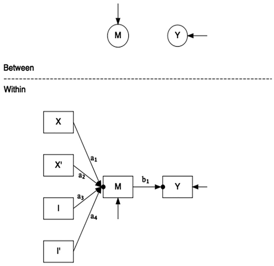Although not shown in the model, one can include direct effects from the composition variables to $Y$ (which are usually labeled c). Following Stapleton et al. (2016), one might label this model “within cluster” because only the hypothesized structure at the within (or individual) level is modeled. The model is also what Preacher et al. (2010) call a 1-1-1 model, which indicates that the structural model is specified at the individual level (with nonindependence modeled by including the variances for the endogenous variables at the between level).

Figure 4.

GAPIM mediation model, level 1 structure.

It is possible to simultaneously estimate the structural model at both levels, with modifications. In MSEM (assuming all variables are measured at the individual level), the between-level models the relationship among the group means, whereas the within-level is comprised of group-mean deviated scores (Hox et al., 2018; Muthén, 1994). Although it is a simple matter to include case complexity as a mediator at the between level, the compositional effects at that level present something of a problem because using all four creates a linear dependency, as the group means for X and X′ and for I and I′ are redundant. Thus, Kenny and Garcia (2012), in their discussion of the GAPIM at the group level (GAPIM-G), suggest using the mean of the actor effect and “the average similarity of all n (n–1)/2 pairs” (p. 477) of all group members as group-level predictors (e.g., the group mean of others’ similarity). One then might propose the model depicted in Figure 5.

Figure 5.

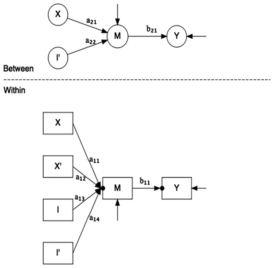
GAPIM mediation model, 2-level structure.

A feature of the model in Figure 5 is that variables included at both levels (Actor Effect, Others’ Similarity) are akin to contextual models, in which both the group mean and group-mean deviated scores predict the outcome (Jak, 2019; Lüdtke et al., 2008; Marsh et al., 2009). Thus, it might be of interest to compare models in which cross-level equality constraints are used. For example, one might wonder if the effect of the mediator is greater at the individual level than that at the between level, and a comparison of model fit statistics between the full (no constraints) and restricted models is easily accomplished within the MSEM framework.

Estimating the Mediation Model

In what follows, the models in Figures 4 and 5 are estimated using R’s lavaan package. However, models with direct effects from the exogenous to outcome variables are not estimated, though that is a relatively simple matter once the logic and mechanics of multilevel mediation from an SEM perspective are understood (see Preacher et al., 2010).

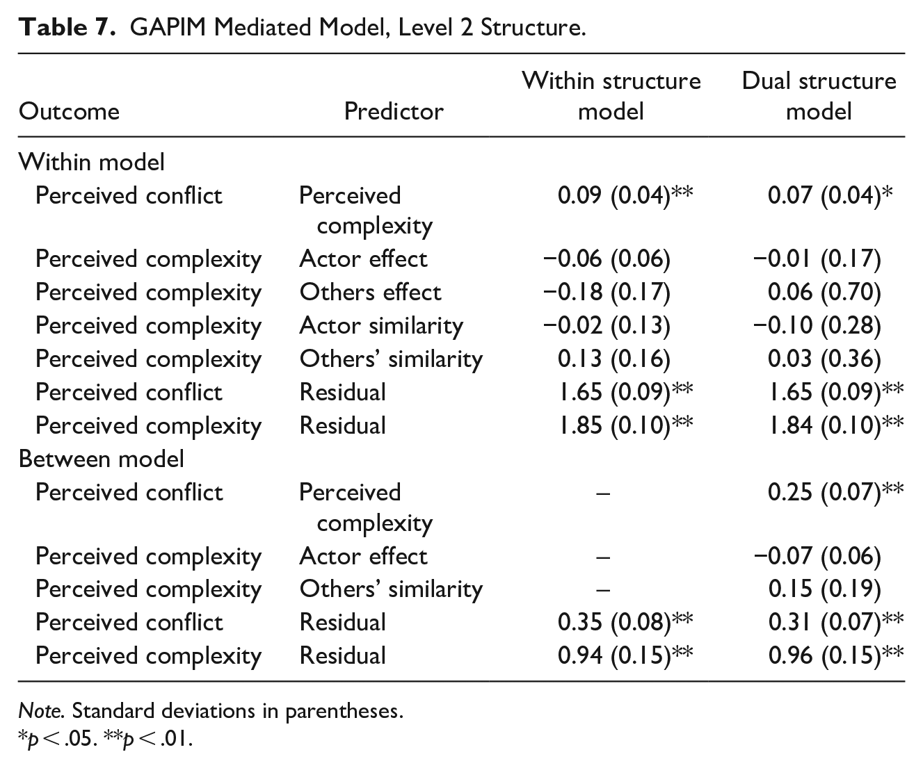
An important item with the model depicted in Figure 5 concerns the two predictors (others effect and actor similarity) that are not included in the between level. Most MSEM software, including R’s lavaan and Mplus, model a within-level predictor at the between level by default, even if that variable is not explicitly included in the between-level structure. This is done for several reasons, one of which is to keep the same structure for the covariance matrices at both levels and, practically, it allows for the estimation of the ICC for those variables. To override the default, one must specifically indicate that the predictor in question varies only at the within level (which prevents it being modeled at the between level). In Mplus, for example, one uses the within command to prevent modeling at the between level, whereas one specifies “fixed.x = FALSE” in the lavaan sem call (not model syntax). Appendix C provides lavaan model syntax and Table 7 contains the model estimates.

Table 7.

GAPIM Mediated Model, Level 2 Structure.

Outcome	Predictor	Within structure model	Dual structure model
Within model
Perceived conflict	Perceived complexity	0.09 (0.04)**	0.07 (0.04)*
Perceived complexity	Actor effect	−0.06 (0.06)	−0.01 (0.17)
Perceived complexity	Others effect	−0.18 (0.17)	0.06 (0.70)
Perceived complexity	Actor similarity	−0.02 (0.13)	−0.10 (0.28)
Perceived complexity	Others’ similarity	0.13 (0.16)	0.03 (0.36)
Perceived conflict	Residual	1.65 (0.09)**	1.65 (0.09)**
Perceived complexity	Residual	1.85 (0.10)**	1.84 (0.10)**
Between model
Perceived conflict	Perceived complexity	–	0.25 (0.07)**
Perceived complexity	Actor effect	–	−0.07 (0.06)
Perceived complexity	Others’ similarity	–	0.15 (0.19)
Perceived conflict	Residual	0.35 (0.08)**	0.31 (0.07)**
Perceived complexity	Residual	0.94 (0.15)**	0.96 (0.15)**

Note. Standard deviations in parentheses.

p < .05. **p < .01.

Results indicate that the Level 1 mediation has a significant and positive effect of the mediator (perceived complexity) on the outcome (perceived conflict) but none of the composition variables are related to the mediator. The ICCs for both endogenous variables are significant and substantial. The dual structure model shows no significant associations at the within level but the between level shows that perceived complexity predicts conflict and that the gender actor effect predicts perceived complexity. Model fit statistics reveal that the dual structure model fits the data well, $χ^{2}$ (6) = 3.48, p = .75, whereas the estimate is $χ^{2}$ (5) = 13.43, p < .01 for the level 1 mediation model.¹⁵ Given the results, one might consider estimating a model with only the between mediation structure and variances for the endogenous variables at the within level, which is akin to what Stapleton et al. (2016) label the shared construct model.

GAPIM Simulations

In this section, results of GAPIM simulations, focusing primarily on power, Type I error, and performance are provided. The issues of power and Type I error are well known; performance assesses the variability of the sample estimates to the population parameter (Morris et al., 2019). As with most simulations, the purpose is to identify relevant design features and statistical qualities that suggest best practices for model estimation given the research question of interest. Two issues stand out regarding the GAPIM. The first is the distribution of the composition variable of interest and the second the degree of nonindependence in the outcome variable. Each is addressed in turn below.

Compositional Skewness

GAPIM estimates are likely affected by the distribution of the composition variable across groups, which in some cases (e.g., laboratory studies of zero-history groups) is within the researcher’s control and in others, including the juries from the ATDP, there is little or no control. The observed composition variable (i.e., gender) is used to create the other three GAPIM terms which, as noted, are the others effect, actor similarity, and others’ similarity; the latter two of which are product-based interaction terms. In the case of a dichotomous composition variable, one may create an orthogonal design, similar to those used in controlled experiments, in which there are equal numbers of groups for each combination of the composition characteristic in question. For example, there are four possible gender combinations (assuming gender is binary) for 3-person groups: 0 males, 1 male, 2 males, and 3 males. The consequence of an orthogonal design is that the GAPIM interaction terms, which are products involving the main effects, are not correlated with the main effects. The actor and others effects are typically correlated as are the two interaction terms. Among other things, nonorthogonal designs produce correlated predictors that inflate standard errors, which reduces statistical power.

Compositional orthogonality is difficult to achieve under the best of circumstances and provides an unrealistic baseline for simulations. Instead, one might approach the problem in terms of the degree of skewness of the composition variable in the population from which study participants and groups are sampled. The problem is akin to that described in the social decision scheme literature (Stasser, 1999), in which the distribution of initial preferences or opinions (e.g., whether a defendant in a criminal trial is guilty) for sample groups is a function of the preference distribution in the population. The odds of randomly sampling any one of the r possible combinations for n-person groups follows the binomial distribution. When the composition variable of interest is assumed evenly distributed in the population, then most samples (assuming a large enough sample) will consist of relatively few groups with just one type of participant; most groups will be mixed. For example, the gender composition for a design with 6-person groups randomly sampled from a population in which gender is balanced is 0.016, 0.09, 0.23, 0.31, 0.23, 0.09, and 0.016 for 0 through 6 females, respectively; the distribution of composition is not skewed across groups. The consequence of drawing enough groups at random from a non-skewed distribution is that the correlations among the main effects and their interaction terms are minimized. The distribution of gender in the ATDP is 53%, which implies that the population from which juries were drawn was relatively equally distributed among men and women. Assuming random assignment to court dates and juries, it is not surprising that the majority of the eight-person juries consisted of equal numbers of men and women (22%), five women (25%), or three women (20%). It is also not surprising the correlations among the interaction terms and main effects are small.

When the compositional variable of interest is uneven, however, the corresponding sample distribution is likely to be skewed. For example, as of this writing, women make up 70% of the student population in many of the social and behavioral sciences (Bui, 2018). Applying the binomial distribution to this situation (i.e., the sampling frame consists of 70% women), the distribution of 6-person gender groups is 0.001, 0.1, 0.06, 0.19, 0.32, 0.30, and 0.12 for 0 to 6 females, respectively. Skewed distributions of compositions across groups are likely, depending on the degree of skewness, to increase correlations among GAPIM main effects and interaction terms, which in turn affects both regression estimates and standard errors.

Outcome Variable Nonindependence

The second issue that affects GAPIM estimates is the nonindependence of the outcome variable. Multilevel modeling, by definition, assumes that the outcome is correlated within groups and for a simple 2-level model the variance of Y is partitioned into that attributable to groups and individuals. The ICC, as noted, is the ratio of between-groups to total variance, with higher estimates indicating similar within-group scores and variation in group means. (If all group means were equal then the variance of Y would be attributable entirely to individuals.) It turns out that the ICC is used to calculate the design effect, “which indicates how much the standard errors are underestimated in a complex sample. . . compared to a simple random sample” (Maas & Hox, 2005, p. 86). The design effect is calculated as $1 + (\overset{↼}{N}) - 1 * I C C$ , where $\overset{↼}{N}$ is average cluster or group size, and values of 2 or lower are considered a small effect (Muthén & Satorra, 1995). For example, a study with eight-person groups and an ICC of 0.30 for the outcome variable yields a design effect of $1 + (8 - 1) * . 30 = 2.4$ , which is larger than 2. The consequence is that the design effect increases as the ICC increases, which means, “as the groups become more internally homogeneous, little added information will be gained from additional individuals within each group” (Heck & Thomas, 2015, p. 387). More to the point, holding group size and the number of groups constant, an increase in the ICC for the outcome reduces the effective sample size, which influences standard errors (Hox et al., 2018).

Given the preceding, a set of simulations were conducted on the full GAPIM model to evaluate model performance under a range of conditions. In addition to group size (4, 6, and 8) and number of groups (25, 50, 75, and 100), which are standard features of multilevel simulations; here medium (0.30) and large (0.50) effect sizes are used for the GAPIM predictors (Cohen, 1988),¹⁶ (b) intraclass correlation (ICC) values of 0.10 and 0.25 for the outcome, and (c) sampling ratios of 0.5 and 0.7 for compositional skewness (assuming a binary variable). The sampling ratio of 0.5 approximates a non-skewed distribution of groups over a large number of samples and 0.7 skews the distribution so that groups are more likely to have values of 1 rather than −1. Each condition used 1000 simulations. The R program simr (Green & MacLeod, 2016) was used to simulate data based on the lmer function from the lme4 package (Bates et al., 2015), and SimDesign (Chalmers & Adkins, 2020) was used to run and extract information from the simulations.

Simulation Results

Model performance is evaluated by estimating (a) statistical power, (b) bias, which is the difference between population parameters and mean sample values (Morris et al., 2019), and (c) Type I error rates.

Power: Main effects

Simulations for the GAPIM main effects model reveal acceptable power (approximately 0.80) for the actor effect for virtually all conditions when the effect size is large (0.50); power dips below 0.80 for 25 groups of 4 when the ICC is large and group distribution is skewed. See Figure 6. Power for the medium effect size is acceptable when composition is not skewed and the number of groups is 50 or greater. For skewed group distributions, power is acceptable when the number of groups = 75 or more but in some cases exceeds .80 when the number of groups = 50. In general, one is best served to strive for non-skewed designs to maximize power for the actor effect.

Figure 6.

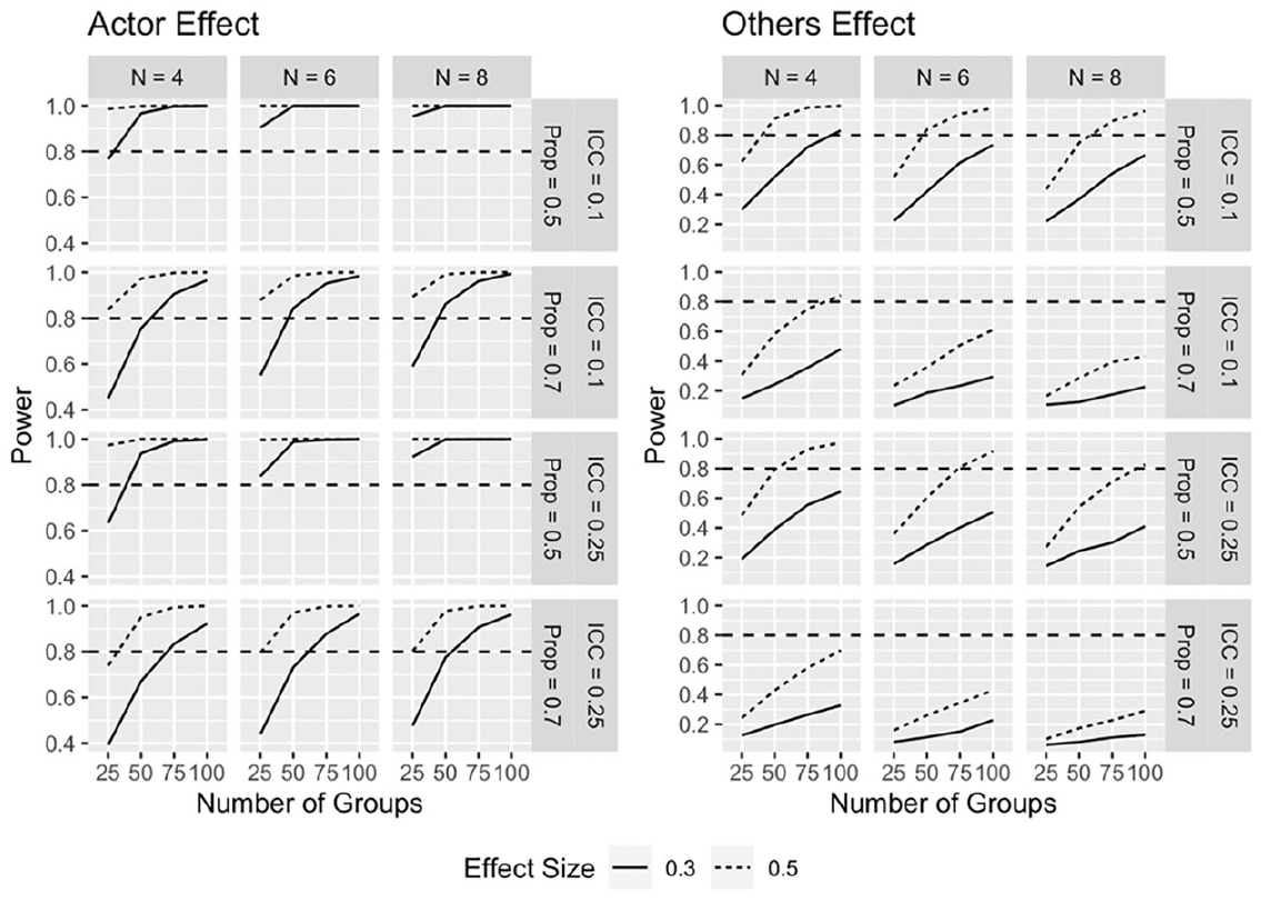
GAPIM power, main effects.

Power for the others effect, in contrast, reveals that the design is underpowered for all conditions where the number of groups = 25 (see Figure 6). In only one case with skewed group composition (group size = 4, number of groups = 100, ICC = 0.1) does power exceed the conventional threshold. In general, power to detect the medium effect size falls below acceptable thresholds in all but one condition, and the large effect size reaches acceptable power with a large number of groups that are not skewed on the compositional variable of interest.

Power: Similarity Effects

As shown in Figure 7, power for the medium actor similarity effect is acceptable for all cases where the ICC = 0.10, the number of groups exceed 75, and the composition is not skewed. Power approaches conventional thresholds for the medium effect when the ICC = 0.25. For the large effect size, power is acceptable in most cases when the number of groups is 50 or greater.

Figure 7.

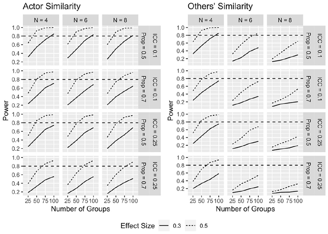
GAPIM power, similarity effects.

The best chance of detecting a medium (0.30) others’ similarity effect, as displayed in Figure 7, is when group size = 4, composition is not skewed, and the ICC = 0.10. The large effect size is significant for all cases where N = 4 and the number of groups exceeds 50. Of potential interest is that power for others’ similarity falls off as group size increases—in only one case (group size = 6, number of groups equals 100, ICC equals 0.10, no skewness) is the test powerful enough by conventional standards.

Bias

Bias measures the difference between population parameters specified in the model and the sample estimates. Estimates for both of the actor and actor similarity effects (see Figure 8) reveal little bias, whereas bias for the other and others’ similarity effects are somewhat more variable (Figure 9). Bias is most pronounced when group size = 8, especially for the others effect, and the direction of bias changes as sample size changes.

Figure 8.

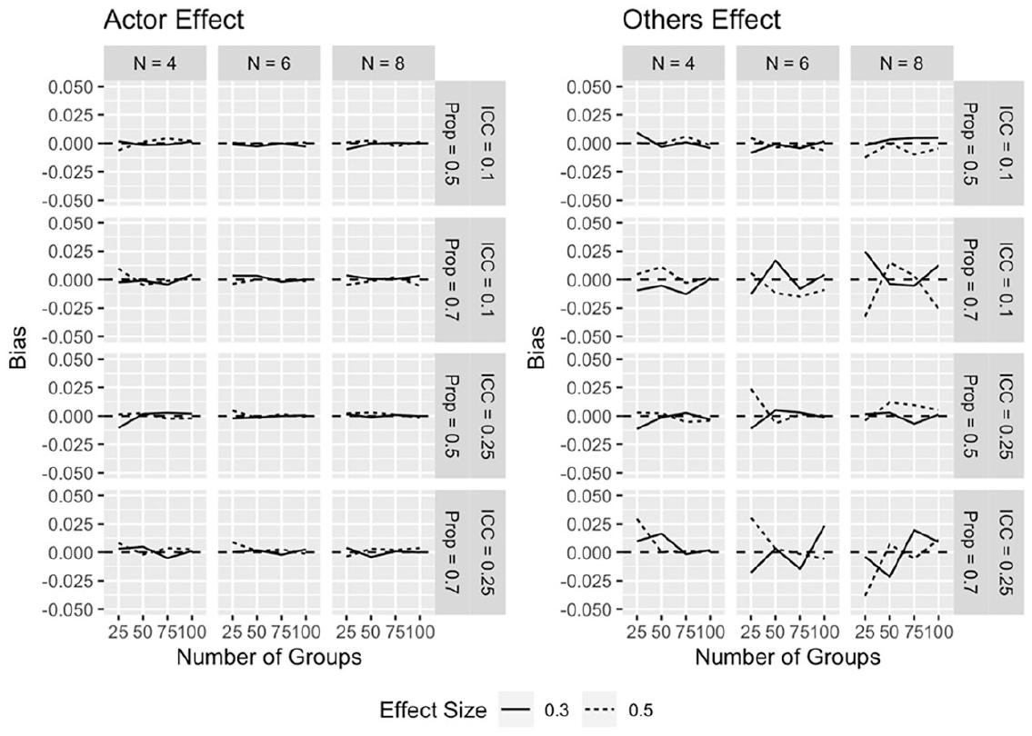
GAPIM bias estimates, main effects.

Figure 9.

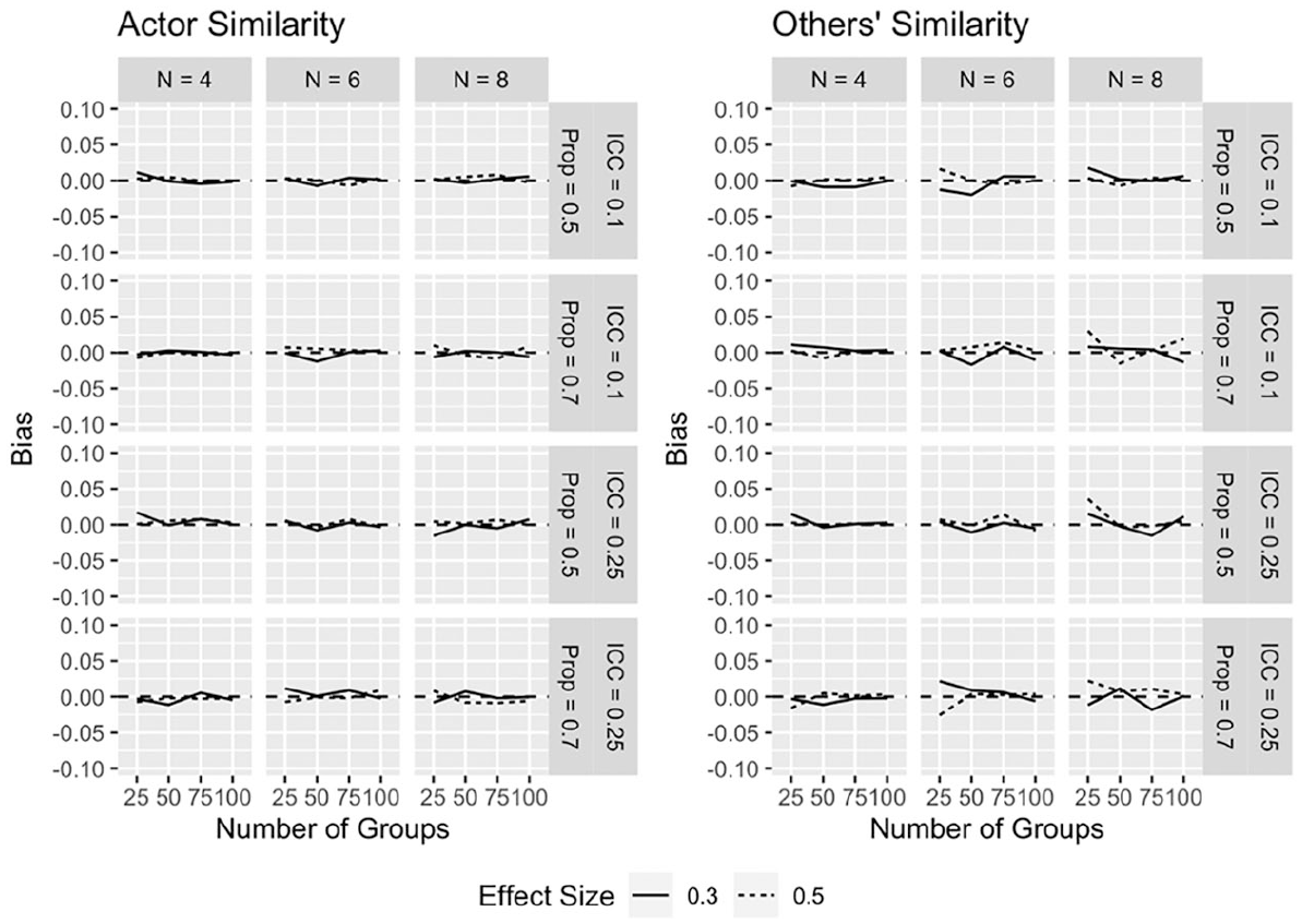
GAPIM bias estimates, similarity effects.

Type I error

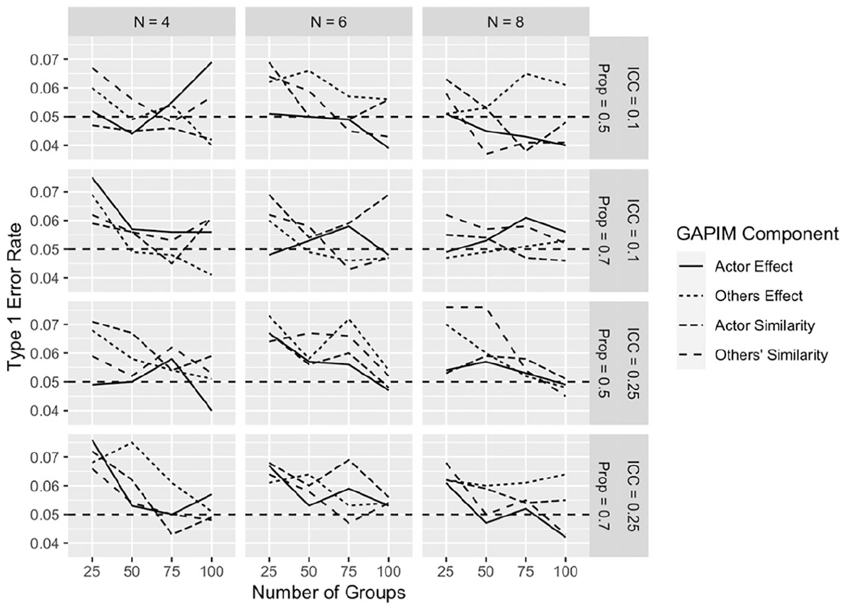
Inspection of Type I error rates (see Figure 10) reveals minimal deviations from the accepted standard of $α$ = .05. Alpha approaches .05 as the number of groups of any size increases though there are exceptions. It appears that alpha inflation occurs consistently when group size = 4 or 6 and the number of groups is 25. Of interest is the comparison of Type 1 error rates when group size equals eight in non-skewed designs. When the ICC = 0.25, inflation is relatively large for all four GAIPM effects, at least compared to the condition in which the ICC = .10. This might be an example of the design effect, in which the standard errors are underestimated as a function of increased homogeneity on the outcome within groups, though the effect decreases as the number of groups increases.

Figure 10.

GAPIM type I error estimates for medium effect size.

Discussion

The main purpose of the paper was to extend the GAPIM beyond multilevel regression. Here, how simple mediation might be incorporated within the GAPIM framework is demonstrated but many other options are possible. The MSEM version also makes incorporating covariates a fairly simply process, and there are likely some cases where one or more of the GAPIM components interact with or are moderated by one or a set of covariates. Finally, one might also incorporate random slopes for the regression paths. For example, using the ATDP model above, one might ask if paths from the actor effect for gender to case complexity, and from complexity to conflict, are consistent across groups.¹⁷

An ancillary purpose of the paper was to evaluate power and performance of the GAPIM multilevel regression model under certain conditions. Here, the focus is on group size, the number of groups, effect size (medium or large), composition skewness (in terms of whether the composition variable of interest is evenly distributed in the population), and degree of nonindependence in the outcome. In summary, the simulations indicate that, all things being equal, one is well advised to have many groups and to balance group composition as equally as possible because doing so generally maximizes power. Group size, however, presents a set of interesting trends in the simulations presented here. In most cases, power is less dependent on group size than the number of groups (Hox et al., 2018); but, overall, power does increase as groups size increases, up to a point. However, the data indicate that the power to detect the other and others’ similarity effects decreases as group size increases; according to the simulations, a non-skewed sample with four-person groups is the most powerful given the conditions simulated here.

The preceding begs the question of why the power to detect the other and others’ similarity effects decreases when group size increases across all conditions (although the decrease is quite small for the others effect when the ICC = 0.10 and the sample is non-skewed). Several related explanations are warranted. A first issue related to power estimates discussed above is the ICC for the predictor variables. As evidenced in Table 1, the average ICCs for the other and others’ similarity effects are quite high, $ρ_{I} = . 86$ and $ρ_{I} = . 73$ , respectively, whereas the ICC for the outcome (perceived conflict) is modest, $ρ_{I} = . 17$ . To my knowledge, only Bliese and Hanges (2004) investigated how power is affected by predictor and outcome ICCs of different magnitudes. Their simulations used rather small ICCs for X and varied the ICCs for the outcome, and found that power was affected to some extent, though the effect depends on group size. To that end, power estimates were simulated for cases with large ICCs for X (ranging from 0.50 to 0.80) and small (0.1–0.25) ICCs for Y. Power is adversely affected when the discrepancy between the two ICCs is largest (i.e., 80 for X and 0.10 for Y) and this is true for the three group sizes (N = 4, 6, and 8) simulated. Power is less affected when the predictor and outcome ICCs are similar (as Bliese and Hanges found). The predictor ICCs in the GAPIM are constructed from observed distributions of the composition variable and, as noted, samples from non-skewed populations minimize within-groups homogeneity on those measures.

The second issue, related to the first, is that both the other and others’ similarity effects have high variance inflation factor (VIF) values in skewed conditions (as well in some of the non-skewed conditions), a function of the correlations among the predictors, which is exacerbated with larger groups. Not only do high VIF values imply increased standard errors for a given regression coefficient, but there are implications regarding the coefficient’s magnitude (see Pedhazur, 1997). Essentially, the order of the predictors in the model influences coefficient estimates. The first term in the model is mostly unaffected by the degree of multicollinearity but subsequent terms are influenced, sometimes dramatically. Bliese and Hanges (2004) suggested more work is needed on understanding the complexities of multilevel models in which interaction terms are included and this paper provides some information on what those effects might be.

The GAPIM is alternative to other, more established models. For example, contextual models evaluate individual and group-level versions of the same construct (Lüdtke et al., 2008). Scores at the individual level are group-mean centered and group means serve as the level 2 predictor; that is, group-mean centering renders the two versions of the variable orthogonal (Enders & Tofighi, 2007). Interest is usually in the group-level effect (e.g., Davis, 1966):

The central question in contextual analysis is whether the aggregated group characteristic has an effect on the outcome variable after controlling for interindividual differences at the individual level. The effects of the L1 characteristic may or may not be of central importance, depending on the nature of the study and the L1 construct. (Lüdtke et al., 2008, p. 204)

The GAPIM’s others effect seems quite similar to the L2 construct in contextual analysis, as the other effect consists of the mean of the other group members on the predictor of interest. Conceptually, however, the difference is that the other affect is akin to the partner effect from the APIM, in which an individual’s outcome is predicted by the average score of his/her colleagues on the variable. Practically, the other affect is a mixed variable (varies both within and between groups) whereas the group mean is a level 2 (between groups) predictor. It is true scores for the others effect are often highly correlated within groups but it addresses a different question compared to those addressed by contextual models.

The interaction terms in the GAPIM reference different types of diversity but others are available. For example, Blau’s (1977) diversity index is a level 2 measure that varies from 0, indicating complete homogeneity, to 1, which is complete heterogeneity. The GAPIM’s interaction terms are level 1 measures that indicate the similarity between an actor and his colleagues (actor similarity) and the homogeneity of all possible pairs of members, excluding self (others’ similarity). Level 2 predictors are especially useful to help explain or account for random intercept and random slope variance (2018). Again, choice of measure is related to conceptual concerns. It should be noted that Coulter (1989) describes a series of inequality/diversity measures that might be of interest beyond what is offered here.

The simulations described here do not address more complicated designs, including mediation. At the very least, the simulations provide some information regarding the relationship between the exogenous GAPIM predictors and the mediator, but more work is needed. As noted, simple mediation has several variants, including the 1-1-1 design (with only variances included at the between level) and one with isomorphic structures at each level (i.e., contextual model). It is unclear how such models perform under conditions described above but it might be the case that performance is related to groups size and composition skewness, as is true of the standard GAPIM. More work is needed in this area.

Composition need not be an obvious characteristic like gender. For example, the analysis above evaluated whether education influences understanding of case evidence and satisfaction with the jury. But education is not an obvious characteristic in most cases, and such information would have to be mentioned during discussion. As such, education and related constructs seem a kind of deep diversity (Cummings et al., 1999; Harrison & Klein, 2007) that require some digging by participants to sort out. And not all deep (or surface level) compositional characteristics are relevant given the task at hand. The mediation example above found a significant actor effect, based on education level, for understanding evidence but no significant effect for the other GAPIM components. It might be that jurors’ education levels were never mentioned, in which case it makes sense for none of the remaining effects, all related to education levels of others, were significant. It might also be the case, as expectation states models suggest (e.g., Balkwell, 1991), that a characteristic has to be salient for the task; if educational backgrounds were made known during discussion then the failure to find significance for the other-related effects is because education level had little bearing on one’s ability to understand evidence. Without having information related to the content of discussion it is hard to know which is the better explanation for the nonsignificant findings.

The preceding focuses value not only on the IPO as a framework for investigating group processes and outcomes, it forces one to investigate how participants learn of deep compositional characteristics and whether those characteristics matter for the task at hand. In principle, the latter (whether a characteristic matters) seems more important and should be assessed first. For example, research has revealed that solution preference (Stasser & Titus, 2003) and expertise (Bottger, 1984) influence process and outcomes. In controlled laboratory studies, one can make these characteristics known, for example, by having groups take a straw vote before deliberation or interaction, or by announcing that one or several participants have worked on similar problems or have scored well on tests that indicate expertise or competence on the task at hand (see Balkwell, 1994). One can make a similar determination about compositional relevance for field studies but it becomes imperative to ascertain if and how such issues become manifest during interaction. Otherwise, there is no way of knowing whether deep compositional characteristics play a role in influencing process and outcomes.

Given that MSEM can address structures at both the within and between levels of analysis, the issue is when either or both levels are relevant. One approach is in terms of collective constructs (Hofmann, 2002; Kozlowski & Klein, 2000), in which emergence plays a key role. Specifically, emergence is defined as a “bottom-up process whereby individual characteristics and dynamic social interaction yield a higher level property of the group” (Kozlowski et al., 2013, p. 584). For example, individuals might experience or perceive some level of satisfaction with process and/or outcomes (Keyton, 1991) but at some point satisfaction might become a group-level characteristic that is qualitatively different from what occurs at the individual level. Emergence, then, is a multilevel process that takes time to develop (Kozlowski et al., 2013). In one sense, individual-level behaviors or cognitions become more similar, which means the group mean is an accurate or reliable indicator of the individual-level measures in question (Bliese, 2000). Thus, a given between-level structure becomes relevant the longer a group works together on a task or series of tasks. And this is true not just for the mediator but for deep level compositional constructs. The between-level structure might not be relevant for zero-history laboratory groups who spend 15 minutes working on a task before members go their separate ways but might very well be relevant for natural groups who have worked together over a series of tasks, for example, a university promotion and tenure committee (Dennis et al., 2006).

Conclusion

The GAPIM is a new and important tool for conceptualizing and evaluating the effect of composition on outcomes of interest. Extending the GAPIM to an MSEM framework provides a wider range of testable models, which should stimulate theorizing based on IPO models of group decision making.

Footnotes

Appendix A

Appendix B

Appendix C

Declaration of Conflicting Interests

The author declared no potential conflicts of interest with respect to the research, authorship, and/or publication of this article.

Funding

The author received no financial support for the research, authorship, and/or publication of this article.

ORCID iD

Joseph A. Bonito

Notes

Author Biography

Joseph A. Bonito (Ph.D., University of Illinois) is Professor of Communication at the University of Arizona, Tucson, AZ. His research interests include small group interaction, multilevel methods, and message analysis.

References

Balkwell

J. W.

(1991). From expectations to behavior: An improved postulate for expectation states theory. American Sociological Review, 56(3), 355–369. https://doi.org/10.2307/2096109

Balkwell

J. W.

(1994). Status. In Foschi

Lawler

E. J.

(Eds.), Group processes: Sociological analyses (pp. 119–148). Nelson-Hall.

Bates

Mächler

Bolker

Walker

(2015). Fitting linear mixed-effects models using Lme4. Journal of Statistical Software, 67(1), 1–48. https://doi.org/10.18637/jss.v067.i01

Blau

P. M.

(1977). Inequality and heterogeneity: A primitive theory of social structure (1st ed.). Free Press.

Bliese

P. D.

(2000). Within-group agreement, non-independence, and reliability: Implications for data aggregation and analysis. In Klein

K. J.

Kozlowski

S. W. J.

(Eds.), Multilevel theory, research, and methods in organizations: Foundations, extensions, and new directions (pp. 349–381). Jossey-Bass.

Bliese

P. D.

Hanges

P. J.

(2004). Being both too liberal and too conservative: The perils of treating grouped data as though they were independent. Organizational Research Methods, 7(4), 400–417. https://doi.org/10.1177/1094428104268542

Bonito

J. A.

(2003). A social relations analysis of participation in small groups. Communication Monographs, 70(2), 83–97. https://doi.org/10.1080/0363775032000133755

Bottger

P. C.

(1984). Expertise and air time as bases of actual and perceived influence in problem-solving groups. Journal of Applied Psychology, 69(2), 214–221. https://doi.org/10.1037/0021-9010.69.2.214

Bui

(2018). https://www.npr.org/sections/money/2014/10/28/359419934/who-studies-what-men-women-and-college-majors

10.

Chalmers

R. P.

Adkins

M. C.

(2020). Writing effective and reliable Monte Carlo simulations with the SimDesign package. The Quantitative Methods for Psychology, 16(4), 248–280. https://doi.org/10.20982/tqmp.16.4.p248

11.

Cohen

(1988). Statistical power analysis for the behavioral sciences (2nd ed.). Routledge.

12.

Cole

D. A.

Maxwell

S. E.

(2003). Testing mediational models with longitudinal data: Questions and tips in the use of structural equation modeling. Journal of Abnormal Psychology, 112(4), 558–577. https://doi.org/10.1037/0021-843x.112.4.558

13.

Cook

W. L.

Kenny

D. A.

(2005). The actor-partner interdependence model: A model of bidirectional effects in developmental studies. International Journal of Behavioral Development, 29(2), 101–109. https://doi.org/10.1080/01650250444000405

14.

Coulter

(1989). Measuring inequality: A methodological handbook. Westview Press.

15.

Cummings

S. M.

Long

J. K.

Peterson-Hazan

Harrison

(1999). The efficacy of a group treatment model in helping spouses meet the emotional and practical challenges of early stage caregiving. Clinical Gerontologist, 20(1), 29–45. https://doi.org/10.1300/j018v20n01_04

16.

Curran

P. J.

Bauer

D. J.

(2007). Building path diagrams for multilevel models. Psychological Methods, 12(3), 283–297. https://doi.org/10.1037/1082-989x.12.3.283

17.

Davis

J. A.

(1966). The campus as a frog pond: An application of the theory of relative deprivation to career decisions of college men. American Journal of Sociology, 72(1), 17–31. https://doi.org/10.1086/224257

18.

Dennis

A. R.

Valacich

J. S.

Fuller

M. A.

Schneider

(2006). Research standards for promotion and tenure in information systems. MIS Quarterly, 30(1), 1–12. https://doi.org/10.2307/25148714

19.

Enders

C. K.

Tofighi

(2007). Centering predictor variables in cross-sectional multilevel models: A new look at an old issue. Psychological Methods, 12(2), 121–138. https://doi.org/10.1037/1082-989x.12.2.121

20.

Green

MacLeod

C. J.

(2016). Simr: An R package for power analysis of generalized linear mixed models by simulation. Methods in Ecology and Evolution, 7(4), 493–498. https://doi.org/10.1111/2041-210x.12504

21.

Hannaford

P. L.

Hans

V. P.

Munsterman

G. T.

(2000). Permitting jury discussions during trial: Impact of the Arizona reform. Law and Human Behavior, 24(3), 359–382. https://doi.org/10.1023/a:1005540305832

22.

Harrison

D. A.

Klein

K. J.

(2007). What’s the difference? Diversity constructs as separation, variety, or disparity in organizations. Academy of Management Review, 32(4), 1199–1228. https://doi.org/10.5465/amr.2007.26586096

23.

Heck

R. H.

Thomas

S. L.

(2015). An introduction to multilevel modeling techniques: MLM and SEM approaches using Mplus (3rd ed.). Routledge.

24.

Hofmann

D. A.

(2002). Issues in multilevel research: Theory development, measurement, and analysis. In Rogelberg

S. G.

(Ed.), Handbook of research methods in industrial and organizational psychology (pp. 247–274). Blackwell.

25.

Hox

J. J.

Moerbeek

van de Schoot

(2018). Multilevel analysis: Techniques and applications. Routledge.

26.

Jak

(2019). Cross-level invariance in multilevel factor models. Structural Equation Modeling: A Multidisciplinary Journal, 26(4), 607–616. https://doi.org/10.1080/10705511.2018.1534205

27.

Kenny

D. A.

(2018). Reflections on the actor-partner interdependence model. Personal Relationships, 25(2), 160–170. https://doi.org/10.1111/pere.12240

28.

Kenny

D. A.

Garcia

R. L.

(2012). Using the actor-partner interdependence model to study the effects of group composition. Small Group Research, 43(4), 468–496. https://doi.org/10.1177/1046496412441626

29.

Kenny

D. A.

Kashy

D. A.

Cook

W. L.

(2006). Dyadic data analysis. Guilford Press.

30.

Kenny

D. A.

Ledermann

(2010). Detecting, measuring, and testing dyadic patterns in the actor–partner interdependence model. Journal of Family Psychology, 24(3), 359–366. https://doi.org/10.1037/a0019651

31.

Keyton

(1991). Evaluating individual group member satisfaction as a situational variable. Small Group Research, 22(2), 200–219. https://doi.org/10.1177/1046496491222004

32.

Kozlowski

S. W. J.

Chao

G. T.

Grand

J. A.

Braun

M. T.

Kuljanin

(2013). Advancing multilevel research design: Capturing the dynamics of emergence. Organizational Research Methods, 16(4), 581–615. https://doi.org/10.1177/1094428113493119

33.

Kozlowski

S. W. J.

Klein

K. J.

(2000). A multilevel approach to theory and research in organizations: Contextual, temporal, and emergent processes. In Klein

K. J.

Kozlowski

S. W. J.

(Eds.), Multilevel theory, research, and methods in organizations: Foundations, extensions, and new directions (pp. 3–90). Jossey-Bass.

34.

Ledermann

Kenny

D. A.

(2017). Analyzing dyadic data with multilevel modeling versus structural equation modeling: A tale of two methods. Journal of Family Psychology, 31(4), 442–452. https://doi.org/10.1037/fam0000290

35.

Lüdtke

Marsh

H. W.

Robitzsch

Trautwein

Asparouhov

Muthén

(2008). The multilevel latent covariate model: A new, more reliable approach to group-level effects in contextual studies. Psychological Methods, 13(3), 203–229. https://doi.org/10.1037/a0012869

36.

Maas

C. J. M.

Hox

J. J.

(2005). Sufficient sample sizes for multilevel modeling. Methodology, 1(3), 86–92. https://doi.org/10.1027/1614-2241.1.3.86

37.

Marcus

D. K.

Leatherwood

J. C.

(1998). The interpersonal circle at zero acquaintance: A social relations analysis. Journal of Research in Personality, 32(3), 297–313. https://doi.org/10.1006/jrpe.1998.2222

38.

Marsh

H. W.

Lüdtke

Robitzsch

Trautwein

Asparouhov

Muthén

Nagengast

(2009). Doubly-latent models of school contextual effects: Integrating multilevel and structural equation approaches to control measurement and sampling error. Multivariate Behavioral Research, 44(6), 764–802. https://doi.org/10.1080/00273170903333665

39.

Moreland

R. L.

Levine

J. M.

(1992). The composition of small groups. In Lawler

E. J.

Markovsky

Ridgeway

Walker

(Eds.), Advances in group processes (pp. 237–280). JAI Press.

40.

Morris

T. P.

White

I. R.

Crowther

M. J.

(2019). Using simulation studies to evaluate statistical methods. Statistics in Medicine, 38(11), 2074–2102. https://doi.org/10.1002/sim.8086

41.

Muthén

B. O.

(1994). Multilevel covariance structure analysis. Sociological Methods & Research, 22(3), 376–398. https://doi.org/10.1177/0049124194022003006

42.

Muthén

B. O.

Satorra

(1995). Complex sample data in structural equation modeling. Sociological Methodology, 25, 267–316. https://doi.org/10.2307/271070

43.

Muthén

L. K.

Muthén

B. O.

(1998–2017). Mplus user’s guide (8th ed.). Muthen & Muthen.

44.

Pavitt

(2014). An interactive input-process-output model of social influence in decision-making groups. Small Group Research, 45(6), 704–730. https://doi.org/10.1177/1046496414548353

45.

Pedhazur

E. J.

(1997). Multiple regression in behavioral research: Explanation and prediction (3rd ed.). Harcourt Brace College Publishers.

46.

Preacher

K. J.

Zyphur

M. J.

Zhang

(2010). A general multilevel SEM framework for assessing multilevel mediation. Psychological Methods, 15(3), 209–233. https://doi.org/10.1037/a0020141

47.

Proyer

R. T.

Brauer

Wolf

Chick

(2019). Adult playfulness and relationship satisfaction: An APIM analysis of romantic couples. Journal of Research in Personality, 79, 40–48. https://doi.org/10.1016/j.jrp.2019.02.001

48.

Rabe-Hesketh

Skrondal

Pickles

(2004). Generalized multilevel structural equation modeling. Psychometrika, 69(2), 167–190. https://doi.org/10.1007/bf02295939

49.

Rosseel

(2012). lavaan: An R package for structural equation modeling. Journal of Statistical Software, 48(2), 1–36. https://doi.org/10.18637/jss.v048.i02

50.

Ryu

West

S. G.

(2009). Level-specific evaluation of model fit in multilevel structural equation modeling. Structural Equation Modeling A Multidisciplinary Journal, 16(4), 583–601. https://doi.org/10.1080/10705510903203466

51.

Stapleton

L. M.

Yang

J. S.

Hancock

G. R.

(2016). Construct meaning in multilevel settings. Journal of Educational and Behavioral Statistics, 41(5), 481–520. https://doi.org/10.3102/1076998616646200

52.

Stasser

(1999). A primer of social decision scheme theory: Models of group influence, competitive model-testing, and prospective modeling. Organizational Behavior and Human Decision Processes, 80(1), 3–20. https://doi.org/10.1006/obhd.1999.2851

53.

Stasser

Titus

(2003). Hidden profiles: A brief history. Psychological Inquiry, 14(3–4), 304–313. https://doi.org/10.1080/1047840x.2003.9682897

54.

Tran

Simpson

J. A.

(2009). Prorelationship maintenance behaviors: The joint roles of attachment and commitment. Journal of Personality and Social Psychology, 97(4), 685–698. https://doi.org/10.1037/a0016418

55.

Zhang

Zyphur

M. J.

Preacher

K. J.

(2009). Testing multilevel mediation using hierarchical linear models: Problems and solutions. Organizational Research Methods, 12(4), 695–719. https://doi.org/10.1177/1094428108327450

Extending the Group Actor-Partner Interdependence Model: MSEM Applications

Abstract

Keywords

Overview

Modeling Group Composition

GAPIM Submodels

Estimating the GAPIM

Categorical Predictor

Continuous Predictor

Extending the GAPIM: An SEM Approach

Estimating the Mediation Model

GAPIM Simulations

Compositional Skewness

Outcome Variable Nonindependence

Simulation Results

Power: Main effects

Power: Similarity Effects

Bias

Type I error

Discussion

Conclusion

Footnotes

Appendix A

Appendix B

Appendix C

Declaration of Conflicting Interests

Funding

ORCID iD

Notes

Author Biography

References