Efficient large-deformation shell elements for the simulation of electromechanical coupling effects in incompressible dielectric elastomers

Abstract

So-called electro-active polymers are not only capable of undergoing very large deformations, but they also exhibit different electromechanical coupling effects due to their dielectric or electrostrictive characteristics. In the present paper the sub-class of dielectric elastomers is studied; in particular, we focus on thin dielectric elastomer shells, which undergo large deformations under an applied electric field. We develop a framework for the modeling and subsequent efficient simulation of thin structures made from incompressible dielectric elastomers. A thermodynamically consistent phenomenological continuum model based on the free energy density is adapted imposing the kinematic assumptions of Kirchhoff-Love shells in combination with including the thickness deformation and the electric field as independent unknown fields. To make the formulation accessible to finite element simulations, existing non-linear elastic shell mixed finite elements are extended to the present hyperelastic electromechanically coupled formulation for dielectric elastomer shells. Computational results of the shell theory are compared to three-dimensional results validating the proposed modeling and numerical simulation methodology, and showing high accuracy already for coarse finite element discretizations of the shell.

1. Introduction

The present paper is concerned with dielectric elastomer solids and structures. These materials are a sub-class of elastic dielectrics, for which Toupin (1956) has been among the very first to present a general theory. Since the ground-breaking paper by Toupin (1956) there has been a vast amount of contributions to the further development of the theory of elastic dielectrics, see for example, Pao (1978), Prechtl (1982a, 1982b), and Maugin (1988). Dielectric elastomers are soft rubber-type materials; they are contracted, when an electric field is applied at electrodes attached to two surfaces of the dielectric material and—as they are typically incompressible—this “squeezing” results in large deformations perpendicular to the direction of the applied electric field. Hence, dielectric elastomers can be used as soft actuating devices, see Choi et al. (2005), Carpi et al. (2005, 2007), and Arora et al. (2007) for examples, and Gu et al. (2017) for a survey on soft robotics using dielectric elastomer actuators.

A common concept to modeling of dielectric elastomers considers the total stress tensor and the augmented free energy function, by means of which ponderomotive forces, which are the sole source of actuation in dielectric elastomers, are accounted for. The free energy function is composed of two parts, one is purely elastic and one is purely electric, see among others Pao (1978), Dorfmann and Ogden (2005), Gao et al. (2011), or Mehnert et al. (2016).

Concerning the numerical simulation of dielectric elastomer solids and structures, the finite element method is often the method of choice. Solid elements for general three-dimensional problems have been developed and studied in the literature for some time. Exemplarily, we mention the contributions by Vu et al. (2007), Gao et al. (2011), Skatulla et al. (2012), Park et al. (2012), Zäh and Miehe (2015), Mehnert et al. (2018), Pechstein (2020), and Kadapa and Hossain (2020).

However, in many practical applications actuating devices made of dielectric elastomers constitute themselves as thin film actuators. Examples for such thin film actuators are for example, a peristaltic pump (Lotz et al., 2009), a buckling pump (Klinkel et al., 2013), a spherical gripper (Bishara and Jabareen, 2019), or a thin helical actuator (Kadapa and Hossain, 2020). Although computing solutions for thin film actuators is possible with solid elements, see for example, Pechstein (2020) and Kadapa and Hossain (2020), numerical simulations using solid elements are often not only expensive, but may result in numerical instabilities or locking. Alternatively, thin film actuators can be modeled in the well established framework of structural mechanics as plates and shells. Such an approach may either be implemented by means of electromechanically coupled solid shell elements or directly in the two-dimensional framework of plate and shell theory, for which in the present case mechanical degrees of freedom must be augmented with proper electrical ones to account for electromechanical coupling directly in the two-dimensional theory.

Without discussing any details, we refer to Libai and Simmonds (2005), Berdichevsky (2009), and Vetyukov (2014a) for modeling and also numerical simulation of purely elastic plates and shells undergoing large deformations. Concerning the case of shells made of hyperelastic soft materials, which is of particular interest for the present paper, we mention only Kiendl et al. (2015) and Duong et al. (2017) and further refer to literature cited therein. The latter two references present isogeometric shell formulations, which we do not wish to adopt in the numerical scheme used in the present paper. Concerning numerical simulation of electro-elastic plates and shells—not necessarily restricted to dielectric elastomers—we mention Ortigosa and Gil (2017) discussing electro-elastic coupling of dielectric elastomers, Poya et al. (2018) addressing also diverse failure phenomena, for example, pull-in instability and formation of wrinkles, and further contributions to the topic by Su et al. (2018) and Greaney et al. (2019). A solid shell formulation for dielectric elastomer shells has been presented by Klinkel et al. (2013), in which solid shell elements with a linear approximation of the electric potential through an element thickness has been proposed with the possibility of using multiple elements through the thickness. For special geometries, analytic considerations and structured grids were successfully employed, see for example, Liu et al. (2021) for a toroidal membrane, or Mishra et al. (2023) for a cylindrical dielectric shell. Such approaches are however not directly applicable to shells of general geometry. Haddadian and Dadgar-Rad (2023) developed a seven parameter shell theory for dielectric elastomer shells involving a Taylor series expansion of the electric field through the shell thickness. Finally, we also refer to contributions to modeling and simulation of electroactive plates and shells from our own group; in particular, Krommer et al. (2016) and Vetyukov et al. (2018) for piezoelectric plates and shells, Staudigl et al. (2018) and Hansy-Staudigl et al. (2019) for dielectric elastomer plates, and Hansy-Staudigl and Krommer (2021) for electrostrictive polymer plates.

Apart from the solid shell approach, a major challenge in the design of finite elements for two-dimensional shell models is the necessity of continuously differentiable surfaces and also deformations. In the present contribution, we develop a two-dimensional shell model for hyperelastic dielectric elastomer shells, and we design efficient coupled mixed finite elements. These elements extend an elastic shell element developed first by Neunteufel and Schöberl (2019, 2021) using a constitutive model based on the Koiter energy to incompressible hyperelastic dielectric elastomers undergoing large deformations. The underlying elastic shell formulation developed in this latter reference extends the classic Hellan-Herrmann-Johnson formulation for Kirchhoff-Love plates (see Hellan, 1967; Herrmann, 1967; Johnson, 1973), in which mid-surface displacement and the moment tensor act as independent unknowns. In the proposed formulation, further kinematic quantities describing curvatures, thickness deformation, and the electric field, as well as a Lagrangian multiplier enforcing the incompressibility constraint, are added in an element-local manner. Most importantly, in this formulation mid-surface displacements need not be continuously differentiable in the finite element model, which increases the usability of the shell element greatly.

The present paper is structured as follows. After a brief summary of the three-dimensional theory of incompressible dielectric elastomers, dielectric elastomer shells undergoing large deformations are discussed in detail. First, we review an already existing approach to Kirchhoff-Love plates and shells; then, we derive an extended shell theory with a relaxed Kirchhoff-Love kinematics. In particular, thickness deformation is included, incompressibility is accounted for by a Lagrangian multiplier and the electric field is assumed linear through the shell thickness. Mixed finite elements for this type of electromechanically coupled shells are then developed and tested against three-dimensional solutions, experimental results and results reported in the literature. It will be shown that the thickness deformation and the electric field must be considered as independent unknowns in order to obtain accurate results for thin dielectric elastomer shells.

2. Incompressible dielectric elastomers

The present paper is concerned with modeling and simulation of electroelastic solids and structures in a large-deformation formulation. In particular, we focus on incompressible dielectric elastomers. Nonetheless, the formulation can be easily extended to be also applicable to materials exhibiting constitutive coupling such as piezoelectricity and electrostriction as well as to ferroelectric solids. Moreover, different hyperelastic models for incompressible elastomers can be included in a straightforward manner. In modeling electroelastic materials, it is common to account for the speed of sound being essentially smaller than the speed of light, which allows the restriction of the formulation to the electrostatic regime. In the current paper, we moreover assume all velocities to be sufficiently small, such that inertia effects become negligible.

Throughout the following, we employ direct tensor calculus as used by Lurie and Belyaev (2005), with a dot expressing contraction of vectors and tensors, and the double contraction $\mathbf{A}:\mathbf{B}=A_{\mathrm{ij}}{B}_{\mathrm{ij}}$ for second order tensors. In this notation, the dyadic product of two vectors $\mathit{a}$ , $\mathit{b}$ is denoted by $\mathit{ab}$ , with components $(\mathit{ab}{)}_{\mathrm{ij}}=a_i{b}_j$ . In accordance with standard notation, let $\mathit{X}$ denote the coordinates of some material point $P$ in an undeformed reference configuration. After deformation, its spatial coordinates $\mathit{x}$ define the displacement field $\mathit{u}$ in such a way that $\mathit{x}=X+u(\mathit{X})$ . With the derivative with respect to material coordinates ${\nabla }_{\mathit{X}}=\partial /\partial \mathit{X}$ , the deformation gradient is given by $\mathbf{F}=({\nabla }_{\mathit{X}}\mathit{x}{)}^T=\mathbf{I}+({\nabla }_{\mathit{X}}\mathit{u}{)}^T$ . The Jacobi determinant $J=det\mathbf{F}$ measures the local change of volume; when considering incompressible materials, one deduces $J\equiv 1$ throughout the domain. The right Cauchy-Green tensor $\mathbf{C}={\mathbf{F}}^T·\mathbf{F}$ is commonly used to describe local deformations in nonlinear continuum mechanics.

Concerning the electric quantities, we introduce the spatial electric field in the deformed configuration $\mathit{e}$ and the derivative with respect to spatial coordinates ${\nabla }_{\mathit{x}}=\partial /\partial \mathit{x}$ . In simply connected domains, Faraday’s law ${\nabla }_{\mathit{x}}\times \mathit{e}=0$ implies the existence of an electric potential $\varphi$ such that $\mathit{e}=-{\nabla }_{\mathit{x}}\varphi$ . In this work, we consider incompressible isotropic linear dielectric materials, where the dielectric displacement $\mathit{d}$ and the electric field $\mathit{e}$ are related in a linear manner through the material’s electric permittivity $ϵ$ ,

$$\mathit{d}=ϵ\mathit{e}.$$

(1)

In contrast to the mechanical quantities, electric field and dielectric displacement are not limited to the body of interest, but extend to the whole space. Maxwell stresses due to the electric field in surrounding air or vacuum lead to additional boundary forces, see for example, Dorfmann and Ogden (2014). When modeling thin dielectric shells with electrodes on both top and bottom surfaces, these forces can often be neglected: at the interface between dielectric material and conducting material, no surface tractions arise, as the electric field is zero within the conductor. Only at lateral free boundaries, if the dielectric material is surrounded by air, the outside electric field gives rise to surface tractions. For a thorough discussion of this case we refer to Gao et al. (2011), where this effect was quantified. Finally, it is justified to restrict all definitions to the material domain. Here, pull-back operations allow to define the material electric field $\mathit{ℰ}=\mathit{e}·\mathbf{F}$ and material dielectric displacement $\mathcal{D}=J{\mathbf{F}}^{-1}·\mathit{d}$ , and finally

$$\mathcal{D}=Jϵ{\mathbf{C}}^{-1}·\mathit{ℰ}.$$

(2)

Moreover, the material electric field obeys $\mathit{ℰ}=-{\nabla }_{\mathit{X}}\varphi$ . For a detailed introduction to nonlinear electroelasticity we refer to Toupin (1956), Eringen and Maugin (2012), and Dorfmann and Ogden (2005, 2017) among many others.

In the current paper, we propose to model material properties in the framework of thermodynamics, in which perfectly incompressible dielectric materials can be fully characterized through a thermodynamic potential

$$\mathrm{\Psi }={\mathrm{\Psi }}_{\mathrm{me}}(\mathbf{C})-\frac{1}{2}Jϵ\mathit{ℰ}·{\mathbf{C}}^{-1}·\mathit{ℰ},$$

(3)

which is often also denoted as the augmented Helmholtz free energy (cmp. Hansy-Staudigl et al., 2019) or electric enthalpy density (cmp. Miehe et al., 2015). Here, ${\mathrm{\Psi }}_{\mathrm{me}}(\mathbf{C})$ may be any isotropic hyperelastic strain energy function.

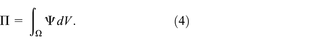
Last, we recall the variational formulation describing the underlying problem; assume, for reasons of simplicity of presentation, that no mechanical external forces act. In their contribution, Miehe et al. (2015) interpret different variational formulations for electro-elastic materials in the framework of thermodynamics. Starting from the minimization of the electro-elastic free energy, augmented by potentials of external loads, a stationary-point condition is derived for the reduced functional

$$\mathrm{\Pi }={\int }_{\mathrm{\Omega }}\mathrm{\Psi }\mathrm{dV}.$$

(4)

Indeed, free energy density and electric enthalpy density $\mathrm{\Psi }$ are linked through a Legendre transform. In our current setting without mechanical external forces acting in $\mathrm{\Omega }$ , displacement field $\mathit{u}$ and electric potential $\varphi$ are to be found such that the kinematic boundary conditions are satisfied exactly, and that $\mathrm{\Pi }$ is minimized over the set of admissible displacement fields, and maximized with respect to all admissible electric potentials.

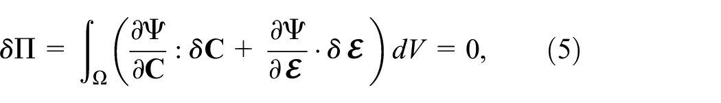
The necessary condition of first order for finding such a saddle point is well-known as principle of virtual work, and reads for admissible virtual displacements $\delta \mathit{u}$ and virtual electric potentials $\delta \varphi$ ,

$$\delta \mathrm{\Pi }={\int }_{\mathrm{\Omega }}(\frac{\partial \mathrm{\Psi }}{\partial \mathbf{C}}:\delta \mathbf{C}+\frac{\partial \mathrm{\Psi }}{\partial \mathit{ℰ}}·\delta \mathit{ℰ})\mathrm{dV}=0,$$

(5)

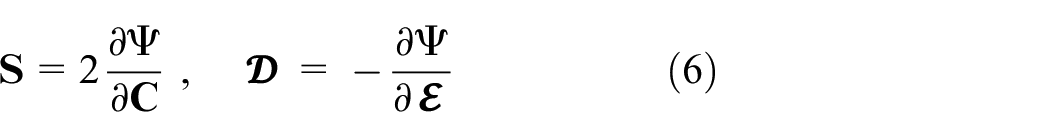
with $\delta \mathbf{C}={\mathbf{F}}^T·({\nabla }_{\mathit{X}}\delta \mathit{u}{)}^T+{\nabla }_{\mathit{X}}\delta \mathit{u}·\mathbf{F}$ and $\delta \mathit{ℰ}=-{\nabla }_{\mathit{X}}\delta \varphi$ . From (5) constitutive relations for the total second Piola-Kirchhoff stress tensor $\mathbf{S}$ and the material electric displacement vector $\mathcal{D}$ can be deduced in the well-known form

$$\mathbf{S}=2\frac{\partial \mathrm{\Psi }}{\partial \mathbf{C}},\mathcal{D}=-\frac{\partial \mathrm{\Psi }}{\partial \mathit{ℰ}}$$

(6)

for compressible materials. The treatment of incompressible materials will be discussed below.

3. Shell models

First, we note that we use the notion shell for thin structures, which are curved in the reference configuration. If the reference configuration is plane, we denote the thin structure as a plate.

The continuum formulations presented above shall now be integrated in a Kirchhoff-Love type thin shell theory, where for the geometric description we use a notation close to Vetyukov (2014b). Therefore, let $\mathcal{S}$ denote the bounded midsurface of the reference configuration—the reference midsurface—of the shell under consideration. With the midsurface unit normal $\mathit{N}$ and the shell thickness $t$ , the volumetric shell domain is defined by

$${\mathrm{\Omega }}_{\mathcal{S}}=\{\mathit{R}+\zeta \mathit{N}:\mathit{R}\in \mathcal{S}\mathrm{and}\zeta \in (-t/2,t/2)\}.$$

(7)

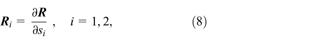
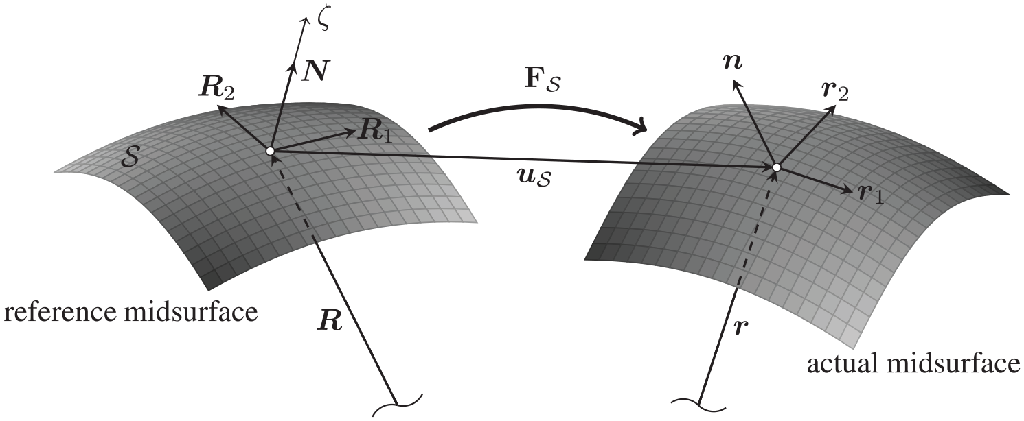
With the position vector $\mathit{R}=\mathit{R}(s_1,s_2)$ of points of the reference midsurface with surface coordinates $s_1$ and $s_2$ , we introduce the covariant tangential base vectors as

$${\mathit{R}}_i=\frac{\partial \mathit{R}}{\partial s_i},i=1,2,$$

(8)

see Figure 1; the corresponding contravariant tangential base vectors are ${\mathit{R}}^1$ and ${\mathit{R}}^2$ . The tangential plane and the curvature of the shell surface in its reference configuration are characterized through the first and second metric tensors $\mathbf{A}$ and $\mathbf{B}$ , which for smooth surfaces are given by

$$\begin{array}{c}\mathbf{A}=\mathbf{I}-\mathit{NN}={\mathit{R}}_1{\mathit{R}}^1+{\mathit{R}}_2{\mathit{R}}^2,\hfill \\ \multicolumn{1}{c}{\mathbf{B}=-{\nabla }_{\mathcal{S}}\mathit{N},}\end{array}$$

(9)

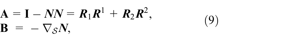
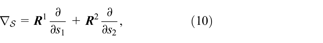
with the surface nabla operator ${\nabla }_{\mathcal{S}}$ ,

$${\nabla }_{\mathcal{S}}={\mathit{R}}^1\frac{\partial }{\partial s_1}+{\mathit{R}}^2\frac{\partial }{\partial s_2},$$

(10)

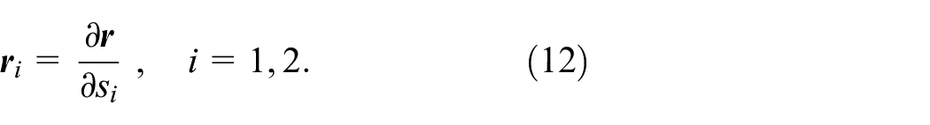
acting in the tangential plane of the surface. Now, let ${\mathit{u}}_{\mathcal{S}}:\mathcal{S}\to R^3$ denote the midsurface displacement, such that $\mathit{r}:=\mathit{R}+{\mathit{u}}_{\mathcal{S}}$ describes the spatial position of the shell midsurface after deformation; the later is denoted as actual midsurface, see also see Figure 1. The surface deformation gradient

$${\mathbf{F}}_{\mathcal{S}}=({\nabla }_{\mathcal{S}}\mathit{r}{)}^T=\mathbf{A}+({\nabla }_{\mathcal{S}}{\mathit{u}}_{\mathcal{S}}{)}^T={\mathit{r}}_1{\mathit{R}}^1+{\mathit{r}}_2{\mathit{R}}^2$$

(11)

Figure 1.

Shell midsurface in the reference configuration (reference midsurface) and shell midsurface in the deformed configuration (actual surface) with position vectors $\mathit{R},\mathit{r}$ , displacement vector ${\mathit{u}}_{\mathcal{S}}$ , surface unit normal vectors $\mathit{N},\mathit{n}$ , and covariant tangential base vectors ${\mathit{R}}_1,{\mathit{R}}_2$ and ${\mathit{r}}_1,{\mathit{r}}_2$ ; $\zeta$ is the Lagrangian thickness coordinate of the shell.

maps the covariant tangential base vectors of the reference midsurface ${\mathit{R}}_1$ and ${\mathit{R}}_2$ onto the covariant tangential base vectors of the actual midsurface ${\mathit{r}}_1$ and ${\mathit{r}}_2$ , which are

$${\mathit{r}}_i=\frac{\partial \mathit{r}}{\partial s_i},i=1,2.$$

(12)

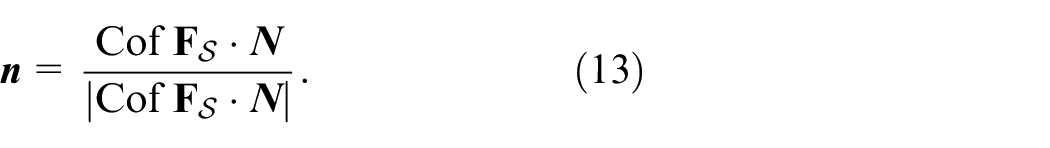
Note that the surface deformation gradient is not invertible, as it is only of rank two; however, its cofactor tensor $\mathrm{Cof}{\mathbf{F}}_{\mathcal{S}}$ is well-defined, see also Neunteufel and Schöberl (2019). The normal vector of the actual midsurface computes as

$$\mathit{n}=\frac{\mathrm{Cof}{\mathbf{F}}_{\mathcal{S}}·\mathit{N}}{|\mathrm{Cof}{\mathbf{F}}_{\mathcal{S}}·\mathit{N}|}.$$

(13)

Due to its degenerate nature, the surface deformation gradient satisfies orthogonality relations with respect to the surface normals,

$${\mathbf{F}}_{\mathcal{S}}·\mathit{N}=\mathit{n}·{\mathbf{F}}_{\mathcal{S}}=0.$$

(14)

The first and second metric tensors of the deformed surface $\mathbf{a}$ and $\mathbf{b}$ are defined through

$$\begin{array}{c}\mathbf{a}=\mathbf{I}-\mathit{nn}={\mathit{r}}_1{\mathit{r}}^1+{\mathit{r}}_2{\mathit{r}}^2,\hfill \\ \multicolumn{1}{c}{{\mathbf{F}}_{\mathcal{S}}^T·\mathbf{b}=-{\nabla }_{\mathcal{S}}\mathit{n},}\end{array}$$

(15)

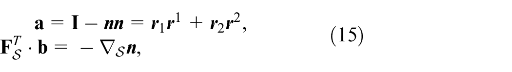
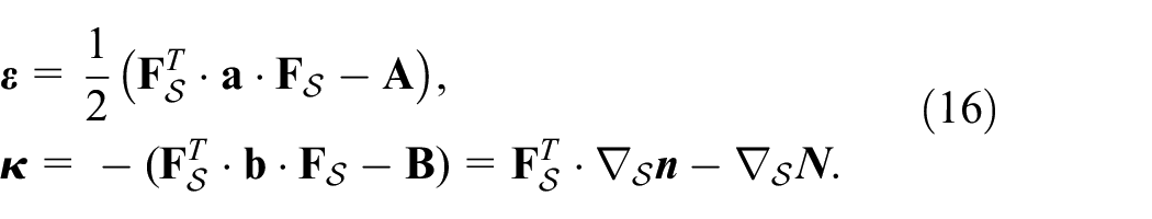
with the tangential contravariant base vectors ${\mathit{r}}^1$ and ${\mathit{r}}^2$ of the actual surface. Now, we define two Green strain measures of the shell surface under the assumptions of Kirchhoff-Love theory, namely a membrane strain $\mathit{\epsilon }$ and a curvature tensor $\mathit{\kappa }$ . Both are symmetric with components in the tangential plane,

$$\begin{array}{c}\multicolumn{1}{c}{\mathit{\epsilon }=\frac{1}{2}({\mathbf{F}}_{\mathcal{S}}^T·\mathbf{a}·{\mathbf{F}}_{\mathcal{S}}-\mathbf{A}),}\\ \multicolumn{1}{c}{\mathit{\kappa }=-({\mathbf{F}}_{\mathcal{S}}^T·\mathbf{b}·{\mathbf{F}}_{\mathcal{S}}-\mathbf{B})={\mathbf{F}}_{\mathcal{S}}^T·{\nabla }_{\mathcal{S}}\mathit{n}-{\nabla }_{\mathcal{S}}\mathit{N}.}\end{array}$$

(16)

Also, we introduce the so-called shifting tensor $\mathbf{\Lambda }$ of the reference configuration,

$$\mathbf{\Lambda }=\mathbf{A}-\zeta \mathbf{B}.$$

(17)

The surface transformation $\mathrm{II}{\mathrm{I}}_{\mathbf{\Lambda }}$ at position $\zeta \ne 0$ different from the shell’s mid-surface refers to the “determinant” of the non full-rank tensor $\mathbf{\Lambda }$ , and can be computed to

$$\mathrm{II}{\mathrm{I}}_{\mathbf{\Lambda }}=\mathit{N}·\mathrm{Cof}\mathbf{\Lambda }·\mathit{N}.$$

(18)

3.1. Kirchhoff-Love plates and shells

We start with a discussion of thin Kirchhoff-Love plates with $\mathbf{B}=0$ and $\mathit{\kappa }=-{\mathbf{F}}_{\mathcal{S}}^T·\mathbf{b}·{\mathbf{F}}_{\mathcal{S}}={\mathbf{F}}_{\mathcal{S}}^T·{\nabla }_{\mathcal{S}}\mathit{n}$ . Under Kirchhoff-Love assumptions, material points on the surface normal $\mathit{R}+\zeta \mathit{N}$ are mapped to the according spatial positions on the deformed normal, $\mathit{r}+\zeta \mathit{n}$ ; from a purely kinematic point of view, this mapping does not account for any thickness deformation. Nonetheless, theories for thin electroelastic plates have been developed based on this mapping. In an approach to dielectric elastomer plates by Staudigl et al. (2018), it was proposed to define the Cauchy-Green tensor based on the Kirchhoff-Love assumptions neglecting higher order terms in the material thickness coordinate $\zeta$ as

$$\begin{array}{c}{\mathbf{C}}_3={\mathbf{C}}_2+C_{\mathrm{NN}}\mathit{NN},\hfill \\ \multicolumn{1}{c}{{\mathbf{C}}_2=\mathbf{A}+2\mathit{\epsilon }+2\zeta \mathit{\kappa }.}\end{array}$$

(19)

To emphasize the three-dimensional nature of the full-rank Cauchy-Green tensor ${\mathbf{C}}_3\equiv \mathbf{C}$ , we use ${\mathbf{C}}_3$ subsequently. Analogously, ${\mathbf{F}}_3$ is used for the full-rank deformation gradient.

For incompressible dielectric elastomers Staudigl et al. (2018), further proposed to compute the thickness component $C_{\mathrm{NN}}$ from the incompressibility condition $J^2=det{\mathbf{C}}_3=1$ resulting into

$$C_{\mathrm{NN}}=\frac{1}{\mathrm{II}{\mathrm{I}}_{C_2}}=\frac{1}{\mathit{N}·\mathrm{Cof}{\mathbf{C}}_2·\mathit{N}},$$

(20)

see also Bonet and Wood (2008), Kiendl et al. (2015), or Duong et al. (2017) for hyperelastic materials. As a last ingredient the through-the-thickness approximation of the material electric field vector $\mathit{ℰ}$ is to be defined. Typically, it is assumed constant and oriented in the direction of the surface normal. For a small thickness $t$ and a given applied voltage $V$ , let ${\mathcal{E}}_0=V/t$ denote the nominal electric field, such that $\mathit{ℰ}=\mathcal{E}\mathit{N}={\mathcal{E}}_0\mathit{N}=V/t\mathit{N}$ , see for example, O’Brien et al. (2009), Vetyukov (2014b), Zhang et al. (2018), or Staudigl et al. (2018). Thus given a representation of ${\mathbf{C}}_3$ in terms of $\mathit{\epsilon }$ , $\mathit{\kappa }$ , $V$ and the thickness coordinate $\zeta$ , a thermodynamic potential for dielectric elastomer plates can be derived by through-the-thickness integration,

$${\mathrm{\Psi }}_{\mathcal{S}}(\mathit{\epsilon },\mathit{\kappa },V)={\int }_{-t/2}^{t/2}\mathrm{\Psi }({\mathbf{C}}_2,V)d\zeta .$$

(21)

Here, the plane stress thermodynamic potential $\mathrm{\Psi }({\mathbf{C}}_2,V)$ is defined as

$$\mathrm{\Psi }={{\mathrm{\Psi }}_{\mathrm{me}}({\mathbf{C}}_3)|}_{{\mathbf{C}}_3={\mathbf{C}}_2+{\mathrm{III}}_{C_2}^{-1}\mathit{NN}}-\frac{1}{2}ϵ\mathrm{II}{\mathrm{I}}_{C_2}{\mathit{ℰ}}_0^2;$$

(22)

its derivative with respect to ${\mathbf{C}}_2$ is the plane stress second Piola-Kirchhoff-type total stress tensor of the plate. The integration can be performed either analytically, neglecting contributions $O({\zeta }^3)$ or higher in $\mathrm{\Psi }({\mathbf{C}}_2,V)$ , or by Gauss integration.

Finally, the principle of virtual work accordingly states

$${\mathrm{\Pi }}_{\mathcal{S}}={\int }_{\mathcal{S}}{\mathrm{\Psi }}_{\mathcal{S}}d\mathcal{S}\to \underset{{\mathit{u}}_{\mathcal{S}}\mathrm{adm}.}{min}.$$

(23)

Note that the electric field is assumed constant and prescribed, and thus is not varied above. Admissibility of the midsurface deformation not only concerns continuity and kinematic boundary conditions; for the curvature tensor $\mathit{\kappa }$ to be well-defined continuous differentiability of ${\mathit{u}}_{\mathcal{S}}$ is necessary. This is an assumption violated by common nodal finite elements, and will be discussed in detail for the presented choice of shell elements.

Solutions for dielectric elastomer plates have been intensively studied in Staudigl et al. (2018) and Hansy-Staudigl et al. (2019) and successfully tested against full 3D solutions.

3.1.1. Extension to shells

Next, we extend the well tested formulation for Kirchhoff-Love plates in a somewhat heuristic, but straightforward manner. Formally, the plane stress thermodynamic potential in (22) with ${\mathbf{C}}_2=\mathbf{A}+2\mathit{\epsilon }+2\zeta \mathit{\kappa }$ is assumed identical to the one for plates. Yet, as $\mathbf{B}\ne 0$ , the curvature tensor is

$$\mathit{\kappa }=-({\mathbf{F}}_{\mathcal{S}}^T·\mathbf{b}·{\mathbf{F}}_{\mathcal{S}}-\mathbf{B}),$$

(24)

and the material electric field is still assumed as constant, $ℰ={ℰ}_{\prime }$ . Through-the-thickness integration involves the surface transformation $\mathrm{II}{\mathrm{I}}_{\mathbf{\Lambda }}$ , such that

$${\mathrm{\Psi }}_{\mathcal{S}}(\mathit{\epsilon },\mathit{\kappa },V)={\int }_{-t/2}^{t/2}\mathrm{\Psi }({\mathbf{C}}_2,V)\mathrm{II}{\mathrm{I}}_{\mathbf{\Lambda }}d\zeta .$$

(25)

As we are dealing with shells with $\mathbf{B}\ne 0$ , we will also adopt a different assumption concerning the electric field as well. To be concise, we assume the dielectric displacement vector $\mathcal{D}$ to be oriented with the surface normal, such that $\mathcal{D}=\mathcal{D}\mathit{N}$ . Then, Gauss’ law of conservation of charges in the reference domain implies that $\mathcal{D}$ is not independent of $\zeta$ , but that the charge density $\mathcal{D}$ multiplied by the surface transformation $\mathrm{II}{\mathrm{I}}_{\Lambda }$ at any $\zeta$ is constant,

$${\mathcal{D}}_0=\mathrm{II}{\mathrm{I}}_{\mathbf{\Lambda }}\mathcal{D},$$

(26)

with a constant ${\mathcal{D}}_0$ . Assuming the coupling of the electrical field with the deformation to be negligible, this implies

$$\mathit{ℰ}={ϵ}^{-1}\mathcal{D}=\frac{{\mathcal{D}}_0}{ϵ\mathrm{II}{\mathrm{I}}_{\mathbf{\Lambda }}}\mathit{N}=\frac{{\mathcal{E}}_0}{\mathrm{II}{\mathrm{I}}_{\mathbf{\Lambda }}}\mathit{N}.$$

(27)

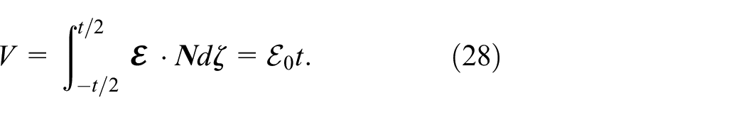
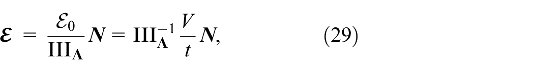
In the computation of the electric field we use the approximation ${\mathrm{III}}_{\mathbf{\Lambda }}^{-1}\approx 1+\zeta \mathrm{tr}\mathbf{B}$ , and find the applied voltage $V$ from integrating through the thickness,

$$V={\int }_{-t/2}^{t/2}\mathit{ℰ}·\mathit{N}d\zeta ={\mathcal{E}}_{0}t.$$

(28)

Therefore, ${\mathit{ℰ}}_0=V/t$ holds, and we propose to use the electric field vector in the Kirchhoff-Love shell theory as

$$\mathit{ℰ}=\frac{{\mathcal{E}}_0}{\mathrm{II}{\mathrm{I}}_{\mathbf{\Lambda }}}\mathit{N}={\mathrm{III}}_{\mathbf{\Lambda }}^{-1}\frac{V}{t}\mathit{N},$$

(29)

which approximates the electric field in an uncoupled electrostatic problem for a small thickness-to-curvature ratio. This implies that ${\mathcal{E}}_0$ must be replaced with ${\mathrm{III}}_{\mathbf{\Lambda }}^{-1}{\mathcal{E}}_0$ in (22).

3.2. Incompressible dielectric elastomer shells

At first glance, the above transition from dielectric elastomer plates to shells is a direct one. Allowing for a second metric tensor $\mathbf{B}\ne 0$ in all derivations leads to common shell formulations for (hyper-)elastic solids, and the extension (29) by a non-constant electric field in the direction of the surface normal seems straightforward. Various authors have however reported inconsistent behavior of such shells as curvature increases. We cite O’Brien et al. (2009), McGough et al. (2014), and Zhang et al. (2018), where the authors superimposed a constant electric field in thickness direction to various available shell elements. Large deviations from either measurements or fully coupled three-dimensional simulations occurred whenever curvature increased, even for initially plane surfaces. Recently, Haddadian and Dadgar-Rad (2023) presented a shell element with an independent approximation of the electric field vector through the thickness. In the current contribution, we propose not only to consider the electric field as non-constant in $\zeta$ , but also to include the thickness deformation in the kinematic description. A novel shell formulation is derived under these assumptions.

For actual shells we introduce the thickness deformation directly as an independent unknown within a relaxed Kirchhoff-Love kinematics in the sense that material points on the surface normal $\mathit{R}+\zeta \mathit{N}$ are mapped to spatial points on the surface normal $\mathit{n}$ of the deformed surface by means of

$$\mathit{R}+\zeta \mathit{N}\to \mathit{R}+\mathit{u}+z(\zeta )\mathit{n}.$$

(30)

The thickness deformation is, at this point, not assumed constant through the thickness, but depends on the material thickness coordinate via $z(\zeta )$ . However, for the current deductions, we assume that the shear induced by this kind of thickness stretch is negligible, such that

$${\nabla }_{\mathcal{S}}z\approx 0,z\prime :=\frac{\partial z}{\partial \zeta }\ne 0.$$

(31)

For this three-dimensional deformation, the deformation gradient can be easily derived. With the three-dimensional nabla operator of the shell ${\nabla }_3={\mathbf{\Lambda }}^{-1}·{\nabla }_{\mathcal{S}}+\mathit{N}\partial /\partial \zeta$ , and assuming (31) one finds

$${\mathbf{F}}_3=\mathbf{\Lambda }·{\mathbf{F}}_{\mathcal{S}}·{\mathbf{\Lambda }}^{-1}+z\prime \mathit{nN},$$

(32)

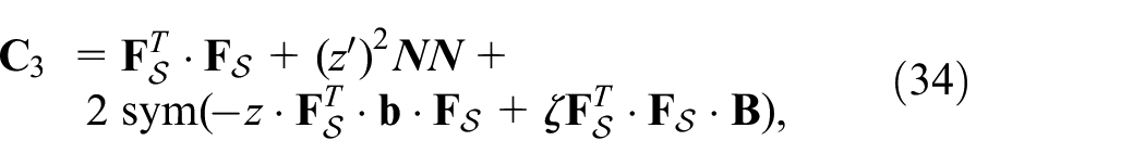
with the shifting tensor of the actual configuration $\mathbf{\Lambda }=\mathbf{a}-z\mathbf{b}$ . This gives rise to the Cauchy-Green tensor ${\mathbf{C}}_3={\mathbf{F}}_3^T·{\mathbf{F}}_3$ ,

$${\mathbf{C}}_3={\mathbf{\Lambda }}^{-1}·{\mathbf{F}}_{\mathcal{S}}^T·\mathbf{\lambda }·\mathbf{\lambda }·{\mathbf{F}}_{\mathcal{S}}·{\mathbf{\Lambda }}^{-1}+(z\prime {)}^2\mathit{NN}.$$

(33)

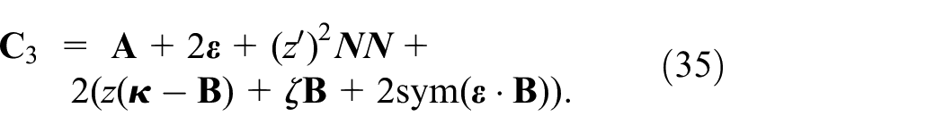
Neglecting terms of order $O({\zeta }^2)$ , $O(z^2)$ , $O(\zeta z)$ or higher, we rewrite

$$\begin{array}{c}{\mathbf{C}}_3={\mathbf{F}}_{\mathcal{S}}^T·{\mathbf{F}}_{\mathcal{S}}+{(z\prime )}^2\mathit{NN}+\hfill \\ \multicolumn{1}{c}{2\mathrm{sym}(-z·{\mathbf{F}}_{\mathcal{S}}^T·\mathbf{b}·{\mathbf{F}}_{\mathcal{S}}+\zeta {\mathbf{F}}_{\mathcal{S}}^T·{\mathbf{F}}_{\mathcal{S}}·\mathbf{B}),}\end{array}$$

(34)

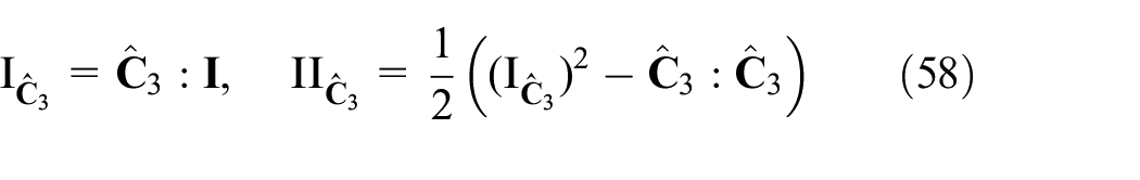
or, in terms of the metric tensors $\mathbf{A}$ and $\mathbf{B}$ of the material surface, as well as the Green strain measures $\mathit{\epsilon }$ and $\mathit{\kappa }$ defined in (16),

$$\begin{array}{c}{\mathbf{C}}_3=\mathbf{A}+2\mathit{\epsilon }+{(z\prime )}^2\mathit{NN}+\hfill \\ \multicolumn{1}{c}{2(z(\mathit{\kappa }-\mathbf{B})+\zeta \mathbf{B}+2\mathrm{sym}(\mathit{\epsilon }·\mathbf{B})).}\end{array}$$

(35)

Note that $\mathit{N}·{\mathbf{C}}_3·\mathit{N}-1=(z\prime {)}^2-1$ is twice the thickness strain. Incompressibility of the material ensures that no volume changes occur, in terms of ${\mathbf{C}}_3$ we observe the condition

$$J=\sqrt{det{\mathbf{C}}_3}=1.$$

(36)

Thereby, the thickness deformation $z$ can, in theory, be made explicit in $\zeta$ . To the best knowledge of the authors, there is no analytic solution for $z$ . Rather, we propose in spirit of well-known displacement-pressure formulations (Sussman and Bathe, 1987; Taylor and Hood, 1973), to introduce a stress $p$ as independent unknown, acting as a Lagrangian multiplier on the incompressiblity constraint (36).

$$\frac{p}{2}\log (det{\mathbf{C}}_3)=0.$$

(37)

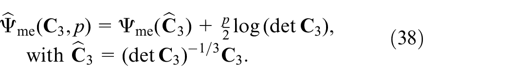
This results in using the alternative hyperelastic potential

$$\begin{array}{c}{\hat{\mathrm{\Psi }}}_{\mathrm{me}}({\mathbf{C}}_3,p)={\mathrm{\Psi }}_{\mathrm{me}}({\hat{\mathbf{C}}}_3)+\frac{p}{2}\log (det{\mathbf{C}}_3),\hfill \\ \multicolumn{1}{c}{\mathrm{with}{\hat{\mathbf{C}}}_3=(det{\mathbf{C}}_3{)}^{-1/3}{\mathbf{C}}_3.}\end{array}$$

(38)

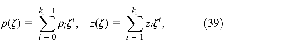
Note that, at this point, the choice of $p$ and $z$ in dependence of the thickness coordinate $\zeta$ is still open. A first idea is certainly to assume $p$ constant through the thickness, and thereby independent of $\zeta$ , while $z=\lambda \zeta$ corresponds to a constant thickness stretch $\lambda =z\prime$ , see for example, Duong et al. (2017) for a discussion of different ways to determine $z$ . However, numerical results will show that the choice $z=\lambda \zeta$ is not sufficient to reproduce the behavior of dielectric elastomer shells accurately. Higher-order approximations of both $p$ and $z$ will be analyzed with respect to their capabilities, where a linear approximation of the stress $p$ and the stretch $z\prime$ will prove sufficient. To allow for unique solvability and an ideal order of approximation in a finite element context it is expedient to have the same number of terms in both expansions. Let therefore, for $k_z>0$ , $p$ and $z$ be defined through

$$p(\zeta )=\sum _{i=0}^{k_z-1}{p}_i{\zeta }^i,z(\zeta )=\sum _{i=1}^{k_z}{z}_i{\zeta }^i,$$

(39)

with $p_i$ and $z_i$ independent of $\zeta$ . We use the terms $p$ and $z$ synonymously for their respective coefficient sets $p_i$ and $z_i$ .

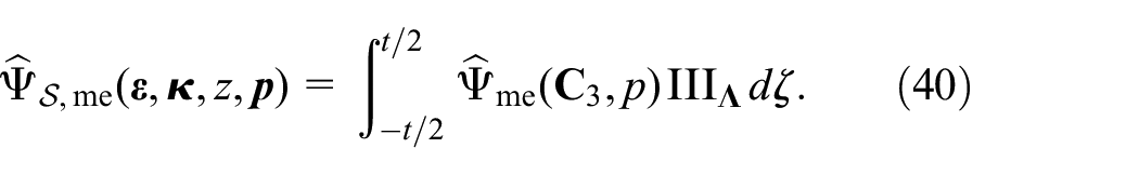
For some given choice of $p$ and $z$ as above, we propose to define a mechanic shell energy density ${\hat{\mathrm{\Psi }}}_{\mathcal{S},\mathrm{me}}$ by inserting these quantities as well as ${\mathbf{C}}_3$ and integrating through-the-thickness in the three-dimensional reference domain accounting for the surface transformation $\mathrm{II}{\mathrm{I}}_{\mathbf{\Lambda }}$ at position $\zeta$ . Then, the mechanic shell energy density contains the contribution by the hyperelastic potential ${\hat{\mathrm{\Psi }}}_{\mathrm{me}}$ by means of

$${\hat{\mathrm{\Psi }}}_{\mathcal{S},\mathrm{me}}(\mathit{\epsilon },\mathit{\kappa },z,\mathit{p})={\int }_{-t/2}^{t/2}{\hat{\mathrm{\Psi }}}_{\mathrm{me}}({\mathbf{C}}_3,p)\mathrm{II}{\mathrm{I}}_{\mathbf{\Lambda }}d\zeta .$$

(40)

3.2.1. Electric field approximation

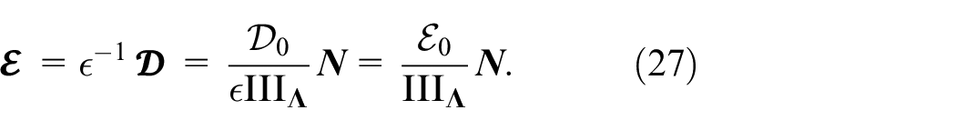
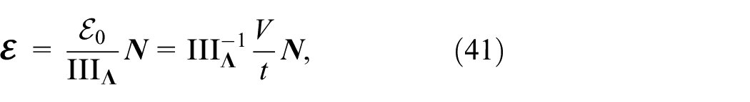
Discussing Kirchhoff-Love shells without an independent thickness deformation, the material electric field $\mathit{ℰ}$ was either assumed constant in thickness direction $\mathit{ℰ}={\mathcal{E}}_0\mathit{N}=V/t\mathit{N}$ , or computed from an uncoupled electrostatic problem as

$$\mathit{ℰ}=\frac{{\mathcal{E}}_0}{\mathrm{II}{\mathrm{I}}_{\mathbf{\Lambda }}}\mathit{N}={\mathrm{III}}_{\mathbf{\Lambda }}^{-1}\frac{V}{t}\mathit{N},$$

(41)

with the area transformation $\mathrm{II}{\mathrm{I}}_{\mathbf{\Lambda }}$ in the reference configuration. In order to account for electromechanical coupling, we first note that with the approximation ${\mathrm{III}}_{\mathbf{\Lambda }}^{-1}\approx 1+\zeta \mathrm{tr}\mathbf{B}$ the electric field

$$\mathit{ℰ}={\mathcal{E}}_0(1+\zeta \mathrm{tr}\mathbf{B})\mathit{N}$$

(42)

has a linear through-the-thickness distribution in the uncoupled problem. In analogy, we set

$$\mathit{ℰ}={\mathcal{E}}_0(1+\zeta {\kappa }_{\mathcal{E}})\mathit{N}$$

(43)

with a constant ${\kappa }_{\mathcal{E}}$ , which is taken as an independent unknown in the solution of the coupled electrostatic problem.

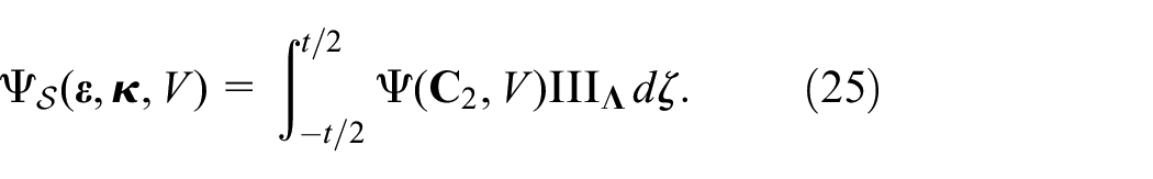
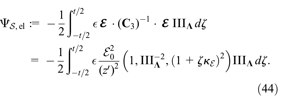
Finally, the electric contribution to the thermodynamic potential (3) including the incompressibilty constraint $J=1$ computes as

$$\begin{array}{c}\multicolumn{1}{c}{{\mathrm{\Psi }}_{\mathcal{S},\mathrm{el}}:=-\frac{1}{2}{\int }_{-t/2}^{t/2}ϵ\mathit{ℰ}·({\mathbf{C}}_3{)}^{-1}·\mathit{ℰ}\mathrm{II}{\mathrm{I}}_{\mathbf{\Lambda }}d\zeta }\\ \multicolumn{1}{c}{=-\frac{1}{2}{\int }_{-t/2}^{t/2}ϵ\frac{{\mathcal{E}}_0^2}{{(z\prime )}^2}(1,{\mathrm{III}}_{\mathbf{\Lambda }}^{-2},{(1+\zeta {\kappa }_{\mathcal{E}})}^2)\mathrm{II}{\mathrm{I}}_{\mathbf{\Lambda }}d\zeta .}\end{array}$$

(44)

Here, the three terms in $(1,{\mathrm{III}}_{\mathbf{\Lambda }}^{-2},{(1+\zeta {\kappa }_{\mathcal{E}})}^2)$ refer to three levels of approximation for the electric field we have introduced; a constant electric field $\mathcal{E}={\mathcal{E}}_0$ , an uncoupled solution $\mathcal{E}={\mathcal{E}}_0{\mathrm{III}}_{\mathbf{\Lambda }}^{-1}$ , and the coupled solution $\mathcal{E}={\mathcal{E}}_0(1+\zeta {\kappa }_{\mathcal{E}})$ . In the example problems, we will consider all three approximations and compare the corresponding solution to each other and to three-dimensional solutions.

3.3. A mixed variational shell formulation

Based on the assumptions and derivations discussed above, we propose the mid-surface displacement ${\mathit{u}}_{\mathcal{S}}$ to be found such that

$$\delta {\mathrm{\Pi }}_{\mathcal{S}}={\int }_{\mathcal{S}}(\delta {\hat{\mathrm{\Psi }}}_{\mathcal{S},\mathrm{me}}+\delta {\mathrm{\Psi }}_{\mathcal{S},\mathrm{el}})d\mathcal{S}=0.$$

(45)

Above, variations $\delta z$ , $\delta p$ , and $\delta {\kappa }_{ℰ}$ do not need to satisfy additional constraints in order to be admissible. The virtual displacement $\delta {\mathit{u}}_{\mathcal{S}}$ needs to satisfy (homogeneous) kinematic boundary conditions; the according virtual membrane strain tensor $\delta \mathit{\epsilon }$ is well-defined for ${\mathit{u}}_{\mathcal{S}}$ and $\delta {\mathit{u}}_{\mathcal{S}}$ weakly differentiable. In order to define the curvature tensor $\mathit{\kappa }$ and its variation $\delta \mathit{\kappa }$ in the same sense, continuous differentiability or $H^2$ continuity is required for ${\mathit{u}}_{\mathcal{S}}$ and $\delta {\mathit{u}}_{\mathcal{S}}$ . This is a trait not provided by standard displacement elements.

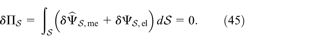
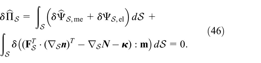
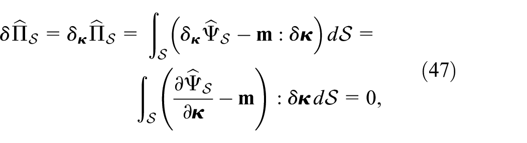
In their original work, Neunteufel and Schöberl (2019) proposed to introduce the moment tensor $\mathbf{m}$ as an independent unknown; hence, as a Lagrangian multiplier for the defining relation for the curvature tensor $\mathit{\kappa }$ in (16). Recently, the same authors proposed to discretize the curvature tensor separately, see Neunteufel and Schöberl (2023). Pechstein et al. (2023) used a similar approach to extend the shell element from linear elastic material models to nonlinear hyperelasticity and electromechanically coupled problems. A corresponding shell formulation amounts to

$$\begin{array}{c}\multicolumn{1}{c}{\delta {\hat{\mathrm{\Pi }}}_{\mathcal{S}}={\int }_{\mathcal{S}}(\delta {\hat{\mathrm{\Psi }}}_{\mathcal{S},\mathrm{me}}+\delta {\mathrm{\Psi }}_{\mathcal{S},\mathrm{el}})d\mathcal{S}+}\\ \multicolumn{1}{c}{{\int }_{\mathcal{S}}\delta (({\mathbf{F}}_{\mathcal{S}}^T·{({\nabla }_{\mathcal{S}}\mathit{n})}^T-{\nabla }_{\mathcal{S}}\mathit{N}-\mathit{\kappa }):\mathbf{m})d\mathcal{S}=0.}\end{array}$$

(46)

This mixed variational formulation explicitly includes the constitutive relation for the moment tensor $\mathbf{m}$ . Setting all variations other than $\delta \mathit{\kappa }$ to zero, such that $\delta \equiv {\delta }_{\mathit{\kappa }}$ , we have

$$\begin{array}{c}\multicolumn{1}{c}{\delta {\hat{\mathrm{\Pi }}}_{\mathcal{S}}={\delta }_{\mathit{\kappa }}{\hat{\mathrm{\Pi }}}_{\mathcal{S}}={\int }_{\mathcal{S}}({\delta }_{\mathit{\kappa }}{\hat{\mathrm{\Psi }}}_{\mathcal{S}}-\mathbf{m}:\delta \mathit{\kappa })d\mathcal{S}=}\\ \multicolumn{1}{c}{{\int }_{\mathcal{S}}(\frac{\partial {\hat{\mathrm{\Psi }}}_{\mathcal{S}}}{\partial \mathit{\kappa }}-\mathbf{m}):\delta \mathit{\kappa }d\mathcal{S}=0,}\end{array}$$

(47)

with ${\hat{\mathrm{\Psi }}}_{\mathcal{S}}={\hat{\mathrm{\Psi }}}_{\mathcal{S},\mathrm{me}}+\delta {\mathrm{\Psi }}_{\mathcal{S},\mathrm{el}}$ . In the absence of $z$ , $p$ , and ${\kappa }_{\mathit{ℰ}}$ , which is the case for Kirchhoff-Love plates and shells without any thickness deformation, we have ${\hat{\mathrm{\Psi }}}_{\mathcal{S},\mathrm{me}}+{\mathrm{\Psi }}_{\mathcal{S},\mathrm{el}}={\mathrm{\Psi }}_{\mathcal{S}}(\mathit{\epsilon },\mathit{\kappa },V)$ from either (22) for plates or (25) for shells.

4. Shell elements

In the mixed variational formulation (46), it is necessary to have both $\mathit{N}$ and $\mathit{n}$ smooth, at least weakly differentiable (and thereby ${\mathit{u}}_{\mathcal{S}}$ twice weakly differentiable or, more classically, piecewise smooth and continuously differentiable), which is not expedient for the design of nodal shell elements. Also, structures involving kinks cannot be treated directly using the above approach.

4.1. A discrete shell formulation

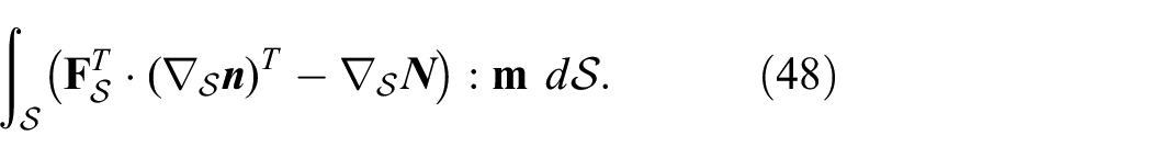
In the spirit of the tangential-displacement normal-normal-stress (TDNNS) method Pechstein and Schöberl (2011, 2017) and Neunteufel and Schöberl (2019) provided a formulation that is valid for both surfaces involving kinks as well as midsurface displacement fields that are not differentiable across element interfaces. We shortly present this idea. Let to this end $\mathcal{T}=\{T\}$ be a triangulation of $\mathcal{S}$ , such that each element is smooth, and kinks are aligned with element boundaries. Let further $ℰ=$ {E} denote the set of all element edges. Further, we assume that the midsurface displacement ${\mathit{u}}_{\mathcal{S}}$ is smooth on each element and continuous across element boundaries, which is usually the case in finite element methods. Consider the term in the total potential ${\hat{\mathrm{\Pi }}}_{\mathcal{S}}$ in (46) that usually requires differentiability of $\mathit{N}$ and ${\mathit{u}}_{\mathcal{S}}$ ,

$${\int }_{\mathcal{S}}({\mathbf{F}}_{\mathcal{S}}^T·{({\nabla }_{\mathcal{S}}\mathit{n})}^T-{\nabla }_{\mathcal{S}}\mathit{N}):\mathbf{m}d\mathcal{S}.$$

(48)

For piecewise smooth displacement fields, (48) can be evaluated in the interior of each element; whereever discontinuities of the normal vector $\mathit{n}$ or $\mathit{N}$ occur, the above formula fails, and another contribution to the work pair (48) will be necessary to model the shell correctly. Finally, we note that for piecewise linear triangulations and midsurface displacements ${\mathit{u}}_{\mathcal{S}}$ , (48) evaluates to zero when restricted to a single element $T$ .

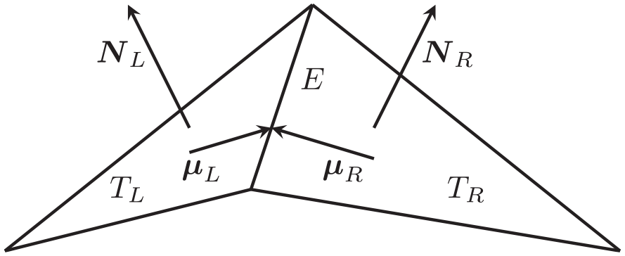
Let now $T_L$ and $T_R$ be two triangles connected through a common edge $E$ . Let further ${\mathit{N}}_R$ , ${\mathit{N}}_L$ denote the surface normals to those triangles, which are not necessarily matching on edge $E$ . Moreover, we define ${\mathbf{\mu }}_R$ and ${\mathbf{\mu }}_L$ as the in-plane edge normals of edge $E$ , compare Figure 2.

Figure 2.

Definition of surface and edge normals for two adjacent elements.

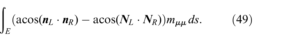
At element boundaries, bending moments are work conjugate to the change in the angle of the two adjacent surface normals. On edge $E$ , let ${\mathbf{\mu }}_R·\mathbf{m}·{\mathbf{\mu }}_R={\mathbf{\mu }}_L·\mathbf{m}·{\mathbf{\mu }}_L=:m_{\mu \mu }$ be the relevant component of the bending moment for a change of angle in the plane normal to $E$ , which is in equilibrium. Its dual, the change of angle during deformation, is given through $\mathrm{acos}({\mathit{n}}_L·{\mathit{n}}_R)-\mathrm{acos}({\mathit{N}}_L·{\mathit{N}}_R)$ , which motivates additional contributions of the form

$${\int }_E(\mathrm{acos}({\mathit{n}}_L·{\mathit{n}}_R)-\mathrm{acos}({\mathit{N}}_L·{\mathit{N}}_R))m_{\mu \mu }\mathrm{ds}.$$

(49)

In Neunteufel (2021), it was shown rigorously that, given bending moments that have a continuous in-plane normal-normal component $m_{\mu \mu }$ as above, the work pair (48) can be evaluated in distributional sense via

$$\begin{array}{c}\multicolumn{1}{c}{\sum _{T\in \mathcal{T}}{\int }_T({\mathbf{F}}_{\mathcal{S}}^T·{({\nabla }_{\mathcal{S}}\mathit{n})}^T-{\nabla }_{\mathcal{S}}\mathit{N}):\mathbf{m}d\mathcal{S}+}\\ \multicolumn{1}{c}{\sum _{E\in \mathcal{E}}{\int }_E(\mathrm{acos}({\mathit{n}}_L·{\mathit{n}}_R)-\mathrm{acos}({\mathit{N}}_L·{\mathit{N}}_R))m_{\mu \mu }\mathrm{ds}.}\end{array}$$

(50)

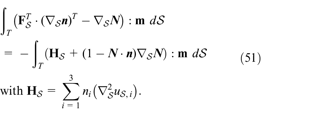
Evaluation through (50) is valid for midsurface displacements that are continuous across element interfaces and smooth within each element. The surface Hessian of the displacement ${\mathbf{H}}_{\mathcal{S}}$ allows a somewhat simpler representation of the surface integrals, see Neunteufel and Schöberl (2019) for a proof,

$$\begin{array}{c}\multicolumn{1}{c}{{\int }_T({\mathbf{F}}_{\mathcal{S}}^T·{({\nabla }_{\mathcal{S}}\mathit{n})}^T-{\nabla }_{\mathcal{S}}\mathit{N}):\mathbf{m}d\mathcal{S}}\\ \multicolumn{1}{c}{=-{\int }_T({\mathbf{H}}_{\mathcal{S}}+(1-\mathit{N}·\mathit{n}){\nabla }_{\mathcal{S}}\mathit{N}):\mathbf{m}d\mathcal{S}}\\ \multicolumn{1}{c}{\mathrm{with}{\mathbf{H}}_{\mathcal{S}}=\sum _{i=1}^3{n}_i\left({\nabla }_{\mathcal{S}}^2{u}_{\mathcal{S},i}\right).}\end{array}$$

(51)

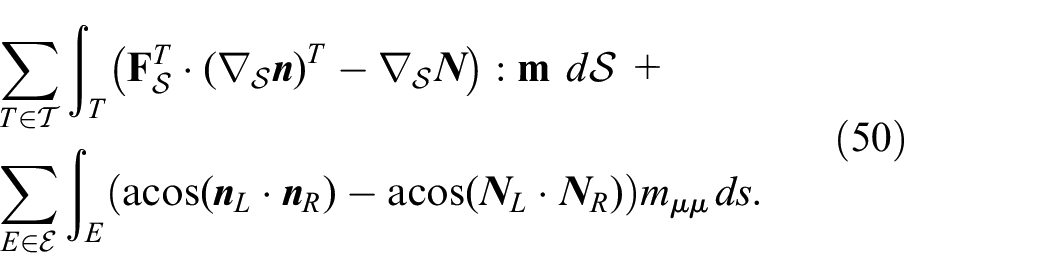
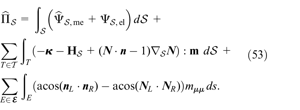
As a result, the variational formulation from (46) is replaced by a formulation that is valid for continuous midsurface displacements and bending moments with continuous in-plane normal-normal component $m_{\mu \mu }={\mathbf{\mu }}_R·\mathbf{m}·{\mathbf{\mu }}_R={\mathbf{\mu }}_L·\mathbf{m}·{\mathbf{\mu }}_L$ . For zero external mechanical forces, the variational formulation reads

$$\delta {\hat{\mathrm{\Pi }}}_{\mathcal{S}}=0,$$

(52)

with the total surface potential

$$\begin{array}{c}\multicolumn{1}{c}{{\hat{\mathrm{\Pi }}}_{\mathcal{S}}={\int }_{\mathcal{S}}({\hat{\mathrm{\Psi }}}_{\mathcal{S},\mathrm{me}}+{\mathrm{\Psi }}_{\mathcal{S},\mathrm{el}})d\mathcal{S}+}\\ \multicolumn{1}{c}{\sum _{T\in \mathcal{T}}{\int }_T(-\mathit{\kappa }-{\mathbf{H}}_{\mathcal{S}}+(\mathit{N}·\mathit{n}-1){\nabla }_{\mathcal{S}}\mathit{N}):\mathbf{m}d\mathcal{S}+}\\ \multicolumn{1}{c}{\sum _{E\in \mathit{ℰ}}{\int }_E(\mathrm{acos}({\mathit{n}}_L·{\mathit{n}}_R)-\mathrm{acos}({\mathit{N}}_L·{\mathit{N}}_R))m_{\mu \mu }\mathrm{ds}.}\end{array}$$

(53)

4.2. Finite element discretization

We shortly comment on the technical aspects of a finite element implementation, such as the choice of approximation spaces, shape functions, or degrees of freedom.

Standard nodal displacement elements can be used for a finite element formulation based on (53). Thus, ${\mathit{u}}_{\mathcal{S}}$ can be discretized using standard nodal elements of order $k$ on each triangular element $T$ . Also quadrilaterals can be treated, but here the definition of shape functions becomes more involved (compare Pechstein and Schöberl (2012) or Neunteufel et al. (2021) for the three-dimensional case), so we do not address this case in the current contribution.

Bending moments $\mathbf{m}$ must be chosen such that they form a stable pair when combined with midsurface displacements, in the sense that an inf-sup condition is satisfied (see Boffi et al. (2013) for a comprehensive analysis on finite element methods for mixed problems). Moreover, the equilibrium constraint $m_{\mu \mu }={\mathbf{\mu }}_R·\mathbf{m}·{\mathbf{\mu }}_R={\mathbf{\mu }}_L·\mathbf{m}·{\mathbf{\mu }}_L$ must be met on shape function level. Finite element basis functions satisfying this constraint on surfaces have been constructed in Neunteufel (2021). As an alternative, it is proposed to use piecewise discontinuous bending moments and add the edge equilibrium constraint via additional Lagrangian multipliers on surface edges. Neunteufel and Schöberl (2019) refer to this workaround as hybridization. In this case, bending moments are discretized using any polynomial basis of order $k-1$ for the tensor components on each triangle $T$ , and also the Lagrangian multipliers are polynomial of order $k-1$ on each edge $E$ in the mesh.

Concerning curvatures, there are no restrictions on the regularity of the finite element function; however it is necessary for $\kappa$ to lie in the tangential plane. In our implementations, we use piecewise polynomial elements of order $k-1$ from a local Regge space, see Neunteufel and Schöberl (2021).

Last, all the additional independent degrees of freedom constituting the through-the-thickness deformation $z$ , stress $p$ , and electric field ${\kappa }_{\mathit{ℰ}}$ do not need to satisfy continuity assumptions, and can be approximated element-wise polynomial. In the computational results presented below, again piecewise in-plane polynomial approximations of order $k-1$ have been used. Having computational efficiency in mind, we note that all these purely local degrees of freedom including curvatures can be eliminated from the global system at assembly time, such that the global system size is not increased.

In Neunteufel and Schöberl (2021), it was shown that the shell element as described above suffers from membrane locking, unless a projection of the membrane strains $\mathit{\epsilon }$ to the Regge space is done. Based on the metric introduced in Regge (1961) for the Einstein field equations, finite elements have been developed since, see Christiansen (2004, 2011) for the lowest order case and Li (2018) for arbitrary order elements. We do not go into details concerning the projection. However, it is important to note that it is a purely local operation that is done on each element and edge in the mesh independently.

5. Examples

Computational results for the proposed shell elements are presented, and compared to solutions of the corresponding fully coupled three-dimensional problem, as well as to three-dimensional models with a prescribed (uncoupled) electric field. Moreover, we compare results of our formulation with experimental data and with existing results from the literature. Full python scripts for reproducing the presented results are publicly available, details can be found in the note on Supplemental Materials at the end of the publication.

5.1. Arc example

Our motivation in choosing the first example problem was to understand the sensitivities of incompressible dielectric elastomer shells under an external applied voltage. In this geometrically very simple problem, we compare the behavior of the full 3D coupled electroelastic model, a 3D model with precomputed electric field, and different shell formulations. Variation of the curvature of the cylindric arc shall show the influence of this parameter on the overall behavior.

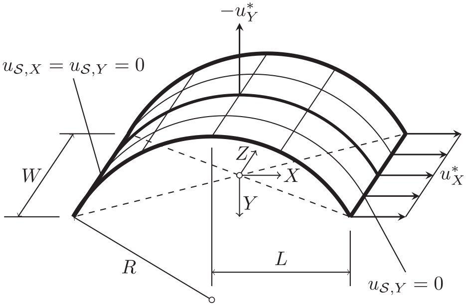
Consider a cylindric arc as shown in Figure 3. Let $\mathcal{S}$ be the mid-surface of a cylindric shell of uniform thickness $t=0.04$  mm and height $W=4$  mm. A section of the cylinder is used, such that the two straight edges are at a respective distance of $2L$ , with $L=2$  mm. We use different radii for the cylinder, ranging from $R=L$ to $R=100L$ . The first choice results in $\mathcal{S}$ a half cylinder, whereas the latter choice implies an almost plane surface $\mathcal{S}$ .

Figure 3.

Geometric setup for the cylindric arc.

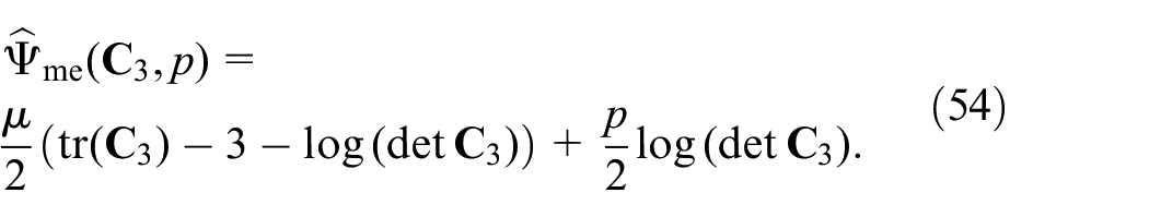
Within this first example, we assume the material to be perfectly isotropic, incompressible, and dielectric with permittivity $ϵ=5{ϵ}_0$ . The hyperelastic potential is assumed to be of Neo-Hooke type with shear modulus $\mu =10\mathrm{kPa}$ . We use the following representation, where the stress $p$ ensures incompressibility

$$\begin{array}{c}\multicolumn{1}{c}{{\hat{\mathrm{\Psi }}}_{\mathrm{me}}({\mathbf{C}}_3,p)=}\\ \multicolumn{1}{c}{\frac{\mu }{2}(\mathrm{tr}({\mathbf{C}}_3)-3-\log (det{\mathbf{C}}_3))+\frac{p}{2}\log (det{\mathbf{C}}_3).}\end{array}$$

(54)

One of the two straight edges located at $X=-L$ is simply supported; in the shell model, midsurface displacements $u_{\mathcal{S},X}=0$ and $u_{\mathcal{S},Y}=0$ are constrained, while in the full three-dimensonal model the according displacements are constrained along a line. The second straight edge at $X=L$ is supported in the sense that $u_{\mathcal{S},Y}=0$ , while the other displacement components are free. Displacement along $Z$ is barred in a single point. We analyze the behavior of the shell when increasing the applied voltage up to $V=360\mathrm{V}$ , which is below the electric breakdown voltage for the considered geometry and material parameters, which is $V=413\mathrm{V}$ . The effect of Maxwell stresses in surrounding air is neglected on the free boundaries.

To compare the different methods with regard to their accuracy, we compute two values for all the setups:

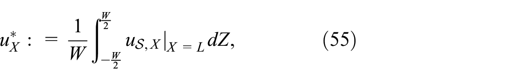
• the mean horizontal displacement of the straight edge at $X=L$ ,

$$u_X^{*}:=\frac{1}{W}{\int }_{-\frac{W}{2}}^{\frac{W}{2}}{u_{\mathcal{S},X}|}_{X=L}\mathrm{dZ},$$

(55)

• the vertical displacement of the center point of the shell surface, located at $X=Z=0$ and $\zeta =0$ ,

$$u_Y^{*}:=u_{\mathcal{S},Y}(X=0,Z=0,\zeta =0).$$

(56)

As will be seen in the results, $u_Y^{*}$ is very sensitive to the different assumptions made in the different shell models.

Different setups are compared; we use the following labels within all the plots.

• 3D. A three-dimensional finite element problem is solved, where an unstructured tetrahedral grid consisting of at least two elements through the thickness is used; displacement and, if applicable, electric potential elements are of order $k=3$ , while the stress $p$ , which acts as a Lagrangian multiplier to ensure incompressibility, is approximated by continuous elements of order $k=2$ (i.e. Taylor-Hood elements).

• shell. A very coarse grid of second order shell elements with a two-parameter expansion for $z$ is used (if not indicated otherwise, $k=k_z=2$ ), the model corresponds to the shell theory developed within this paper.

• KL shell. On the same grid, second order shell elements implementing the Kirchhoff-Love shell theory according to (19) and (20) are implemented, compare also (25).

Concerning the electric field approximations, three variants are identified that apply to all setups.

• E fully coupled. In the three-dimensional simulations, the electric field is approximated on the same mesh at the same polynomial order $k=3$ . In shell formulations, an independent electric degree of freedom is added according to equation (43).

• E uncoupled. In the three-dimensional simulations, the electric field $\mathit{ℰ}$ is precomputed from the uncoupled electrostatic problem in the reference configuration; the displacement is computed consecutively for $\mathit{ℰ}$ . In shell formulations, the electric field is chosen accordingly as (29).

• E constant. In the three-dimensional as well as shell simulations, the material electric field is assumed as $\mathit{ℰ}={ℰ}_{\prime }N$ .

5.1.1. Electric loading

In a first study, the electric load is raised up to $360$  V within 18 load steps. A fixed ratio of $R/L=2$ is compared, which results in an opening angle of $\pi /3$ for the cylindric arc; the initial curvature is certain to affect results.

For this special choice of geometry, the full three-dimensional problem results in a mesh of 23,946 elements, leading to 384,096 degrees of freedom for the displacement, 41,005 degrees of freedom for the stress $p$ , and 128,032 degrees of freedom for the electric field. On the other hand, the surface mesh used for the various shell models consists of 62 triangular elements, and 1723 coupling degrees of freedom including midsurface displacements and (bending) moments on edges.

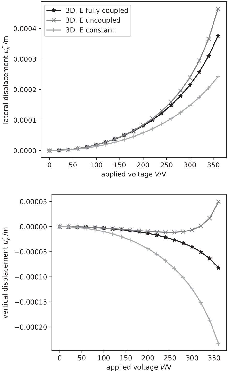
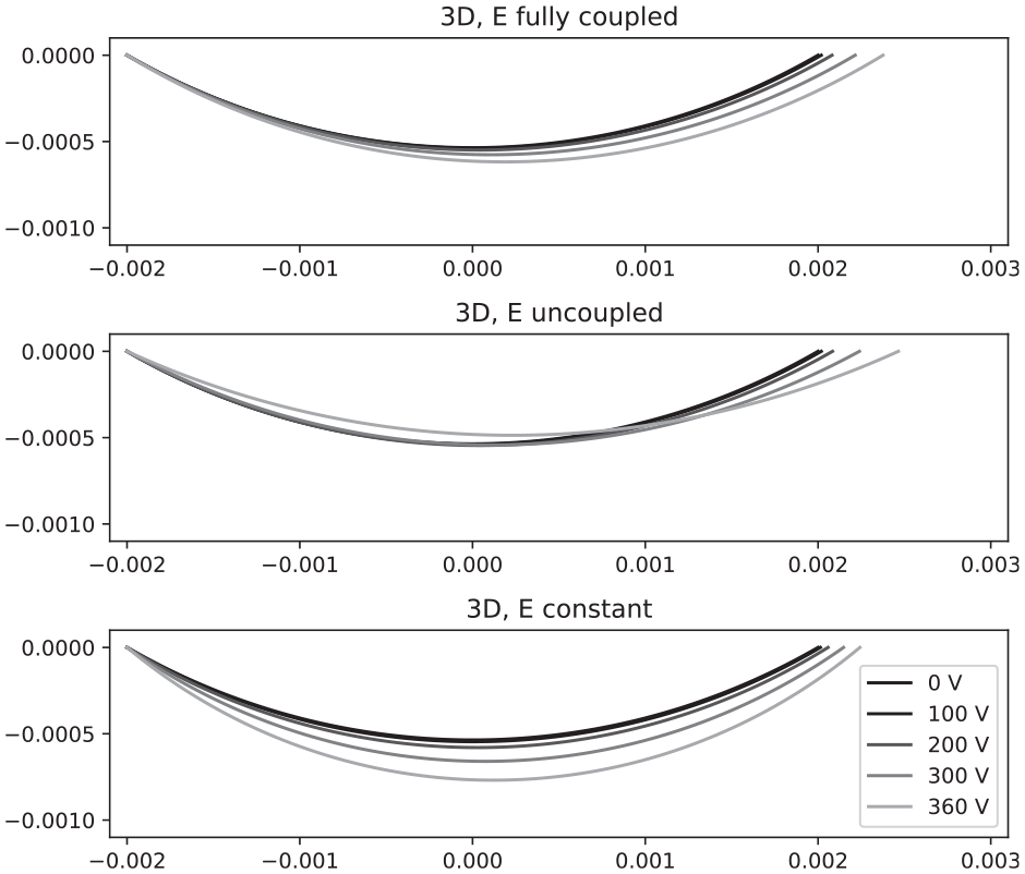
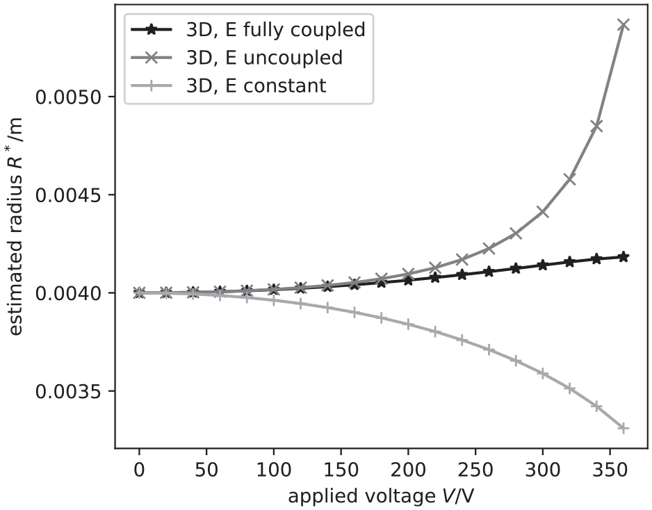
Before analyzing the different shell models, we seek to understand the behavior of the structure in 3D simulations on the tetrahedral mesh. Therefore, we compare results for the horizontal and vertical displacement values $u_X^{*}$ and $u_Y^{*}$ when computing the solution to a fully electromechanically coupled problem, the mechanical problem for the precomputed electric field as well as for constant radial electric field. We observe strongly deviating results, especially in the vertical displacement quantity $u_Y^{*}$ , see Figure 4. This implies great sensitivity of the problem at hand with respect to small variations in the applied electric field. While the precomputed electric field yields valid results within a moderate range of voltages up to approximately 150–200 V, the behavior of the structure under constant $\mathit{ℰ}$ is inherently different already for small voltages. To understand the mechanisms behind the different evolution of these quantities, in Figure 5 the deformation of the shell’s radial center line (indicated bold in Figure 3) is compared for the various settings and voltages. Additionally, we provide the evolution of the cylindric arc’s estimated radius $R^{*}$ in Figure 6. Here, $R^{*}$ is computed by fitting a cylinder through the simply supported edge $-L{\mathit{e}}_X+Z{\mathit{e}}_Z$ , the center point $(\sqrt{R^2-L^2}-R+u_Y^{*}){\mathit{e}}_Y$ , and the supported edge $(L+u_X^{*}){\mathit{e}}_X+Z{\mathit{e}}_Z$ . We find that, while in the case of an uncoupled electric field, the radius is over-estimated, for constant electric field the computed radius is too small. In the framework of shell theories, this implies that impressed moments are not modeled correctly under these kinematic assumptions. Only in the fully coupled simulation, an almost constant observed radius implies that mainly membrane strains are affected through the electric actuation, while very little curvature is introduced. The chosen displacement quantities $u_X^{*}$ and $u_Y^{*}$ are well-suited to monitor these differences.

Figure 4.

Evolution of displacement quantities for $R/L=2$ for three-dimensional simulations with different assumptions on the electric field.

Figure 5.

Evolution of deformation of center line for $R/L=2$ for three-dimensional simulations with different assumptions on the electric field.

Figure 6.

Evolution of the estimated radius $R^{*}$ of the cylindric arc for $R/L=2$ for three-dimensional simulations with different assumptions on the electric field.

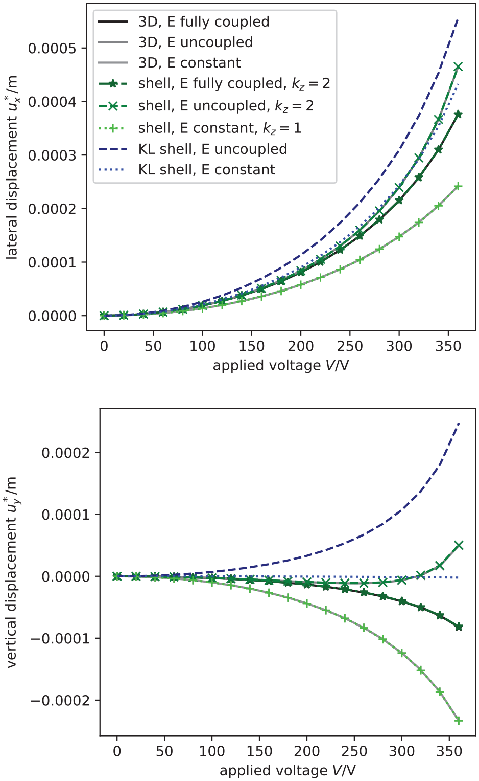
In Figure 7, we compare these horizontal and vertical displacement values $u_X^{*}$ and $u_Y^{*}$ to solutions from various shell formulations. We see that only the proposed shell model including independent degrees of freedom for thickness deformation and variation of the electric field can capture the correct behavior through the whole range of voltages. Electromechanically coupled 3D results and shell results with $k_z=2$ and a coupled electric field coincide, 3D results with an uncoupled electric field and shell results with $k_z=2$ and an uncoupled electric field coincide, and 3D results with a constant electric field coincide with shell results with $k_z=1$ and a constant electric field. Shell models built on classic Kirchhoff-Love shell theory also do not catch the behavior of any of the three-dimensional variants even for small voltages.

Figure 7.

Evolution of displacement quantities for $R/L=2$ comparing different models.

5.1.2. Choice of approximation order

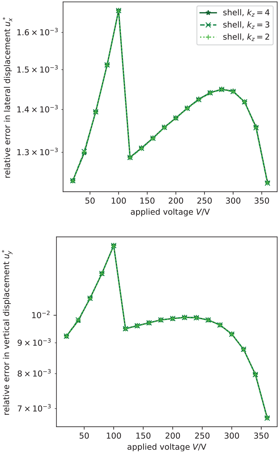
Next, we compare different orders of approximation for the different orders of expansion for $z$ and $p$ (i.e. varying $k_z$ ). To do so, we again consider the case $R/L=2$ and the same meshes as above. In Figure 8, the relative deviation from the fully coupled 3D simulation over voltage is plotted for different approximations; in any case the proposed shell solution is computed with an independent electric field. We see that increasing the order of expansion beyond two has virtually no effect on the quality of the solution, which is to be expected as higher order terms have been neglected within the derivations at several occurances. Over the whole range of voltages, the error is below $2$ % even for point evaluation of ${\mathit{u}}_{\mathcal{S}}$ in the vertical displacement quantity, where the chosen point is not a nodal position in the mesh.

Figure 8.

Relative error in the approximation, as compared to the fully coupled three-dimensional problem. Increasing the order of expansion beyond $k_z=2$ has virtually no effect.

5.1.3. Dependence on curvature

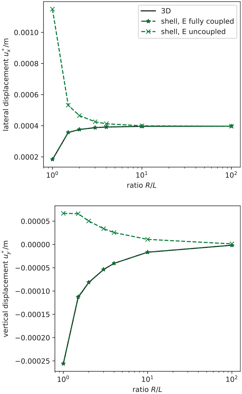
For the next study, the dependence on the initial curvature on the accuracy of the predicted solution is compared. To this end, the ratio $R/L$ is varied within $[1,100]$ . Figure 9 provides the computed displacement quantities at the highest voltage of $V=360$  V. We see that only the proposed shell with independent electric field can reproduce the behavior of the fully coupled 3D model correctly, although the differences become smaller as the initial curvature decreases.

Figure 9.

Comparison of the predicted displacement quantities for different ratio $R/L$ at $V=360\mathrm{V}$ .

5.2. Wrinkling example

In our second example, we seek to compare the proposed shell elements to experimental results. In Mao et al. (2021) a pre-stretched dielectric membrane was subjected to an electric field, which results in the formation of wrinkles. Measurement results presented here are kindly provided by the authors of the latter contribution.

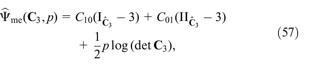
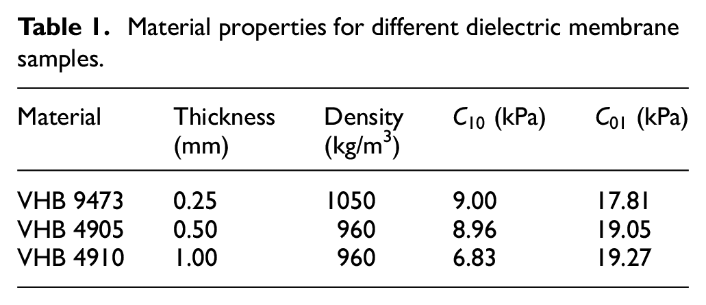
In Mao et al. (2021) dielectric elastomer membranes are pre-stretched and applied to a plane frame of $L_X\times L_Y=100\mathrm{mm}\times 100\mathrm{mm}$ that is aligned with global ${\mathit{e}}_X$ and ${\mathit{e}}_Y$ directions. This pre-stretch is chosen unidirectional and aligned with the frame with ${\lambda }_X=1.5$ and ${\lambda }_Y={\lambda }_X^{-1/2}$ ; hence, for incompressibility the corresponding thickness stretch is ${\lambda }_Z={\lambda }_X^{-1/2}$ . Gravity is acting in $-{\mathit{e}}_Z$ direction. Three different membranes were tested, thickness and material properties are collected in Table 1. The electric permittivity is given as $ϵ=4.12\times {10}^{-11}$  C/Vm for all three membranes; a Mooney-Rivlin hyperelastic potential of the form

$$\begin{array}{l}{\widehat{\mathrm{\Psi }}}_{\mathrm{me}}({\mathbf{C}}_3,p)=C_{10}({\mathrm{I}}_{{\widehat{\mathbf{C}}}_3}-3)+C_{01}({\mathrm{II}}_{{\widehat{\mathbf{C}}}_3}-3)\\ +\frac{1}{2}p\log (\det {\mathbf{C}}_3),\end{array}$$

(57)

is used, where

$${\mathrm{I}}_{{\hat{\mathbf{C}}}_3}={\hat{\mathbf{C}}}_3:\mathbf{I},\mathrm{I}{\mathrm{I}}_{{\hat{\mathbf{C}}}_3}=\frac{1}{2}({({\mathrm{I}}_{{\hat{\mathbf{C}}}_3})}^2-{\hat{\mathbf{C}}}_3:{\hat{\mathbf{C}}}_3)$$

(58)

are the first two invariants of ${\hat{\mathbf{C}}}_3=(det{\mathbf{C}}_3{)}^{-1/3}{\mathbf{C}}_3$ . In order to correctly incorporate the pre-stretch and the resulting pre-stress in our simulation, we first introduce a reference configuration with the dimensions of the pre-stretched membrane $L_X\times L_Y=100\mathrm{mm}\times 100\mathrm{mm}$ . The thickness of the membrane in this reference configuration is assumed to be the one of the original un-stretched membrane $t$ . The in-plane pre-stretch is accounted for multiplicatively by means of ${\mathbf{F}}_{*}={\lambda }_X{\mathit{e}}_X{\mathit{e}}_X+{\lambda }_Y{\mathit{e}}_Y{\mathit{e}}_Y$ and we introduce an elastic right Cauchy-Green tensor as

$${\mathbf{C}}_{3,\mathrm{e}}={\mathbf{F}}_{*}^T·(\mathbf{A}+2(\mathit{\epsilon }+\mathbf{z}\mathit{\kappa }\mathbf{)}\mathbf{)}\mathbf{·}{\mathbf{F}}_{\mathbf{*}}+\mathbf{(}\mathbf{z}\prime {\mathbf{)}}^2\mathit{NN}\mathbf{,}$$

(59)

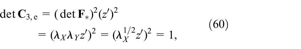
replacing ${\mathbf{C}}_3$ in (57). As the pre-stretched membrane is initially plane, $\mathbf{B}=0$ leads to the somewhat simpler representation above. Note that ${\mathbf{C}}_{3,\mathrm{e}}$ in (59) is not a geometrical right Cauchy-Green tensor; nonetheless, it is used in (57) also in the last term to enforce incompressibility. Say, no electric field and no gravity, but only ${\mathbf{F}}_{*}$ is acting in the pre-stretched reference configuration with original thickness $t$ . Then, no in-plane strain $\mathit{\epsilon }$ and no curvature $\mathit{\kappa }$ result from ${\mathbf{F}}_{*}$ , as long as ${\mathbf{F}}_{*}$ does not result in out-of-plane buckling, which is the case in our problem. Therefore, ${\mathbf{F}}_{*}$ produces no strain, but only a stress in the membrane; the latter is a tension stress in ${\mathit{e}}_X$ direction $({\lambda }_X>1)$ and a compressive stress in ${\mathit{e}}_Y$ direction $({\lambda }_Y<1)$ and corresponds to the actual in-plane stress in the pre-stretched membrane. The incompressibility constraint, which is enforced by means of the pressure term in (57) reads

$$\begin{array}{c}\multicolumn{1}{c}{det{\mathbf{C}}_{3,\mathrm{e}}=(det{\mathbf{F}}_{*}{)}^2(z\prime {)}^2}\\ \multicolumn{1}{c}{=({\lambda }_X{\lambda }_{Y}z\prime {)}^2=({\lambda }_X^{1/2}z\prime {)}^2=1,}\end{array}$$

(60)

for $\mathit{\epsilon }=0$ and $\mathit{\kappa }=0$ , from which $z\prime ={\lambda }_X^{-1/2}={\lambda }_Z$ is found. Hence, the solution due to ${\mathbf{F}}_{*}$ only maps the reference configuration $L_X\times L_Y=100\mathrm{mm}\times 100\mathrm{mm}$ with thickness $t$ used in the numerical simulation onto the actual pre-stretched configuration with the correct thickness $t^{*}={\lambda }_{Z}t$ and with the correct pre-stress; in a second load step gravity and thereafter an electric potential are applied in the simulation.

Table 1.

Material properties for different dielectric membrane samples.

Material	Thickness (mm)	Density (kg/m3)	$C_{10}$ (kPa)	$C_{01}$ (kPa)
VHB 9473	0.25	1050	9.00	17.81
VHB 4905	0.50	960	8.96	19.05
VHB 4910	1.00	960	6.83	19.27

For all computations, half of the domain is discretized, as the wrinkling patterns are observed to be symmetric in Mao et al. (2021). Two different unstructured triangular finite element meshes are used for computations, which are refined towards the physical boundaries of the domain, where singularities and steep gradients are expected. All computations were conducted using third-order elements $(k=3)$ . For the membranes VHB 4905 and VHB 4910, 1138 elements lead to a total count of 50,491 coupling degrees of freedom. Simulating the evolution of wrinkles in the thin membrane VHB 9473 requires a finer mesh consisting of 2534 third-order elements. For this case, the size of the linear system to be solved in each Newton step amounts to 113,071 degrees of freedom.

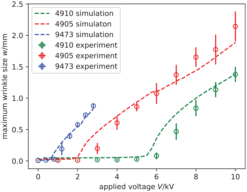
When using the proposed shell formulation with independent electric field, wrinkle sizes can be computed from a quasi-static simulation. In our simulation, the maximum wrinkle size along the symmetric boundary of the membrane is computed. These values are compared to measurements from the experiments in Mao et al. (2021), compare Figure 10. One can see that qualitatively the results coincide, while the critical buckling voltage is lower in the simulations. For the thinnest membrane VHB 9473, at $V=2.9\mathrm{kV}$ no convergence was reached, which is in accordance with measurements.

Figure 10.

Evolution of wrinkle size in pre-stretched dielectric membrane, comparison to measurements (Mao et al., 2021).

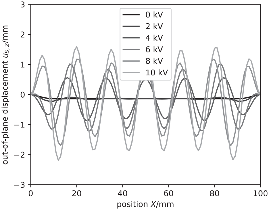
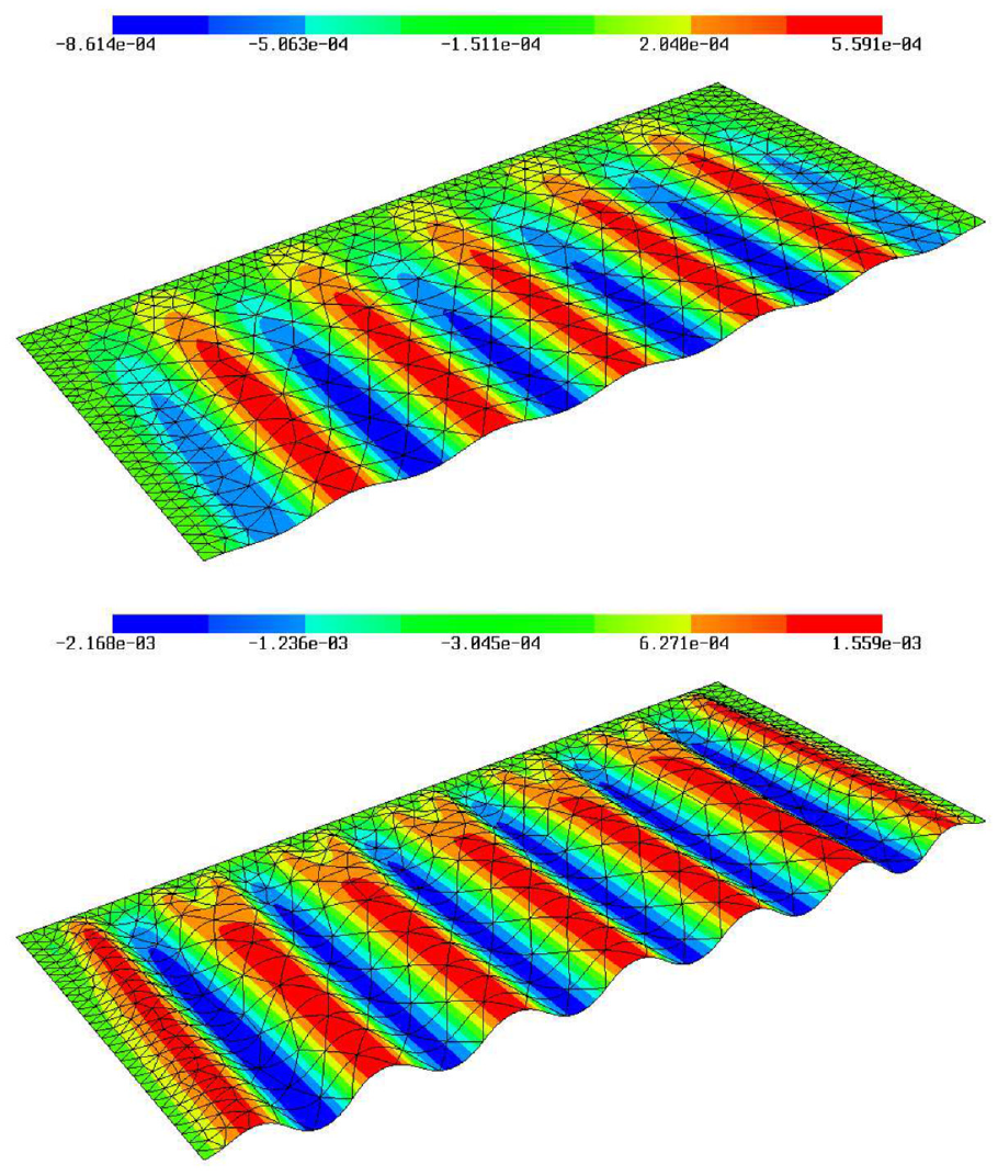
For VHB 4905, the out-of-plane displacment $u_{\mathcal{S},Z}$ is monitored along the center line, see Figure 11. For voltages up to 6 kV, the number and orientation of the wrinkles is in perfect agreement to the measurement results. For higher voltages above 8 kV, an additional pair of wrinkles develops in simulations, which is visible only at the highest voltage of 10 kV in the original measurements. However, the deviation of wrinkle sizes increases at voltages over 6 kV, therefore the sensitivity of measurement results to initial imperfections is certainly relevant in this range. In simulations, it is essential to have enough degrees of freedom, why we chose third-order elements. Additionally, in this range the voltage load steps should be no larger than 125 V to avoid convergence problems. Additionally, the wrinkling pattern obtained in our simulations is depicted in Figure 12. In accordance with experimental findings, small wrinkles are observed at the frame boundaries at high voltages.

Figure 11.

Out-of-plane displacement distribution for pre-stretched dielectric membrane VHB 4905 at different voltages.

Figure 12.

Wrinkling pattern obtained for VHB 4905 at 4 kV (top) and 10 kV (bottom), the color plot shows the deflection $u_{\mathcal{S},Z}$ . At 10 kV, the formation of small wrinkles at the frame boundaries is observed.

We finally note that, when modeling dielectric membranes such as above, viscoelastic effects can, in general, not be neglected. In our computations, no stress relaxation is possible, which leads to higher pre-stresses as observed in experiments. Also, we have not considered the sensitivity of our results with respect to the uncertainty in the material’s stiffness, which is reported in Mao et al. (2021). Our framework for continuum modeling of dielectric elastomers directly allows for the consideration of viscoelastic effects, similar models have been characterized with respect to viscoelastic properties for example, by Ask et al. (2012), Hossain et al. (2015), and Mehnert et al. (2021a, 2021b). Concerning finite element computations, continuum elements or solid shell elements have been proposed, see for example, Büschel et al. (2013) or Bishara and Jabareen (2019). An extension to include viscoelastic properties of these elastomers in a structural mechanics formulation is of considerable interest, and subject of further investigation.

5.3. Dielectric semi-spherical shell

This last example is taken from Kadapa and Hossain (2020). A thin semi-spherical shell of mean radius R = 20 mm and thickness t = 0.5 mm is fully clamped at its circular boundary. The shell is assumed to be made from a dielectric material based on an Arruda-Boyce hyperelastic material law with shear module $\mu =10\mathrm{kPa}$ , cross-link density $N=5$ , and electric permittivity $ϵ=5{ϵ}_0$ . A voltage $V$ is applied to the compliant electrodes located on the inner and outer surface, and raised until breakdown is observed. At a certain voltage, wrinkles form around the clamped edge. In the original reference, wrinkle patterns for a fully coupled 3D simulation were computed.

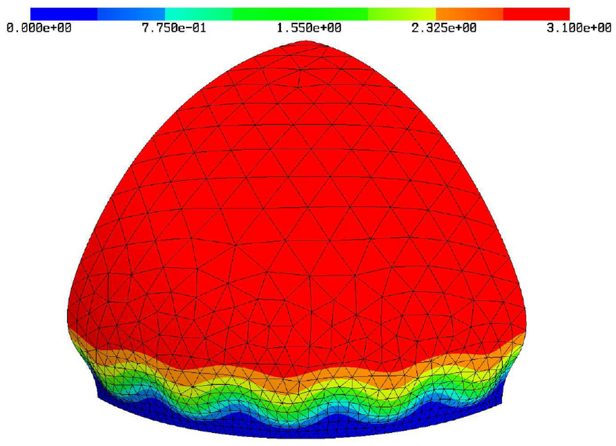
Due to symmetry, only a quarter shell is modeled in the finite element analysis; using spherical coordinates, we have the azimuthal angle $\varphi \in (0,\pi /2)$ as well as the polar angle $\theta \in (0,\pi /2)$ . We use a mesh consisting of 1020 triangular, curved surface elements. Computations were performed using second order elements (i.e. $k=2$ ) with independent electric field (43). In total, 24,280 coupling degrees of freedom are counted. We observe a similar wrinkling pattern as was reported in the original reference Kadapa and Hossain (2020). Five wrinkles form along a quarter of the circumference. The onset of wrinkling was observed at an applied voltage of about V = 5255 V. When exceeding V = 5324 V, the simulation stopped as a different buckling mode was found in the static computations. The pattern observed at V = 5324 V is displayed in Figure 13. Due to a lack of reported actual numerical values in Kadapa and Hossain (2020), we note that the number of wrinkles is identical to the number of wrinkles reported in Kadapa and Hossain (2020) and that buckling/formation of wrinkles occurs at a comparable critical voltage. In any case it should be pointed out that our solution is a static shell solution, whereas the one reported in Kadapa and Hossain (2020) is a dynamic three-dimensional one. Moreover, the thickness deformation in our shell formulation is an internal degree-of-freedom, for which we cannot prescribe a boundary condition. Therefore, the thickness stretch at the clamping is not constrained in our solution, such that the type of clamping we implement allows for a thickness deformation.

Figure 13.

Semi-spherical shell for an applied voltage of V = 5324 V using proposed shell with fully coupled electric field; radial component of midsurface displacement $u_N/\mathrm{mm}$ .

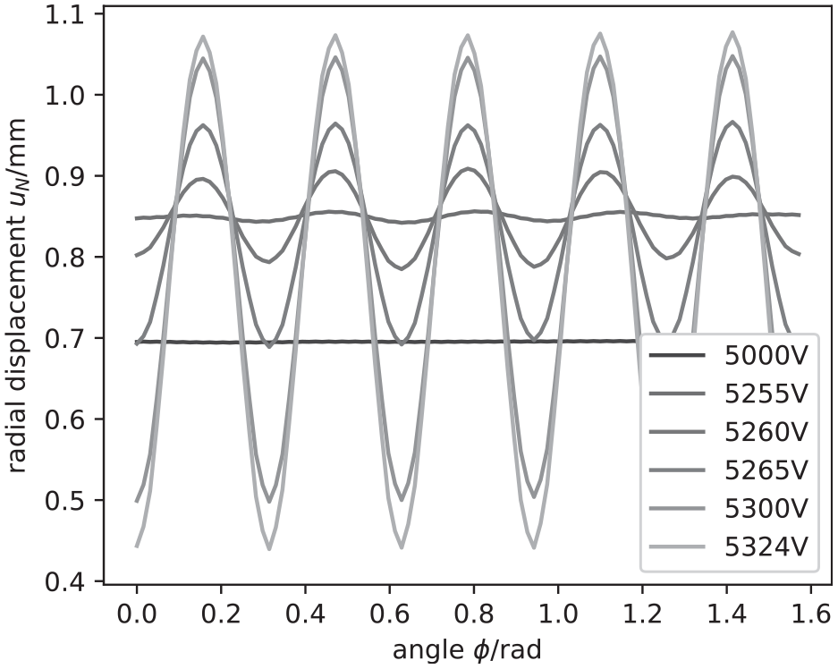
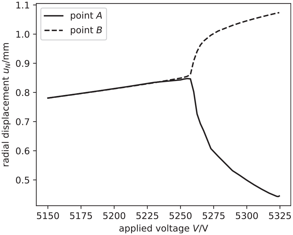
Figures 14 and 15 further capture the evolution of the wrinkling pattern. The radial displacement component $u_N={\mathit{u}}_{\mathcal{S}}·\mathit{N}$ is captured at a uniform polar angle $\theta =\pi /2-\pi /36$ ; in Figure 14 this displacement is plotted for different pre- and post-critical voltages. Moreover, the onset of buckling is clearly visible in Figure 15, where two distinct points $A$ and $B$ , at the same polar angle $\theta =\pi /2-\pi /36$ and azimuthal angles ${\varphi }_A=0$ and ${\varphi }_B=\pi /4$ , are monitored. Again, we have no numerical values from Kadapa and Hossain (2020), but we note that the radial displacement $u_N$ that occurs just before buckling is comparable to values, which can be extracted from plots presented in Kadapa and Hossain (2020).

Figure 14.

Radial component of midsurface displacement $u_N$ for different applied voltages below and above the buckling point.

Figure 15.

Radial component of midsurface displacement $u_N$ at points $A$ and $B$ over applied voltage.

6. Conclusion

Within this article, we have presented a formulation for the description of thin dielectric elastomer shells as oriented material surfaces subject to a relaxed Kirchhoff-Love kinematic assumption. We have seen that, for shells exhibiting curvature in the stress-free reference configuration, thickness deformation cannot be expressed explicitely through the classical deformation measures membrane strain and curvature using plane-stress assumptions. Therefore, a shell theory including the thickness deformations as a separate degree-of-freedom has been developed. Furthermore, it shows that the classical assumption of the electric field being constant and oriented in the direction of the surface normal is not sufficient to describe the electromechanically coupled behavior of dielectric shells. Another independent degree-of-freedom representing the linear variation of the electric field through the thickness is sufficient to reproduce results gained in three-dimensional fully coupled simulations. These additional degrees of freedom do not mar the overall efficiency of the original elastic shell element; they are element-local and can be eliminated at assembly time, and thus do not enlarge the nonlinear system to be solved in each load step. A highly accurate and efficient shell formulation based on nodal displacement and edge-wise moment degrees of freedom is extended to our new formulation. A variety of computational results not only emphasize the capability of the proposed formulation and finite element discretization, but also detect and quantify the sensitivities of thin dielectric shells with respect to common through-the-thickness kinematic assumptions.